Two-sample Categorical data: Testing - University of...
22
Introduction Fisher’s Exact Test The χ 2 test Summary Two-sample Categorical data: Testing Patrick Breheny October 29 Patrick Breheny Biostatistical Methods I (BIOS 5710) 1/22
Transcript of Two-sample Categorical data: Testing - University of...

IntroductionFisher’s Exact Test
The χ2 testSummary
Two-sample Categorical data: Testing
Patrick Breheny
October 29
Patrick Breheny Biostatistical Methods I (BIOS 5710) 1/22

IntroductionFisher’s Exact Test
The χ2 testSummary
Lister’s experiment
In the 1860s, Joseph Lister conducted a landmark experimentto investigate the benefits of sterile technique in surgery
At the time, it was not customary for surgeons to wash theirhands or instruments prior to operating on patients
Lister developed a new operating procedure in which surgeonswere required to wash their hands, wear clean gloves, anddisinfect surgical instruments with carbolic acid
This new procedure was compared to the old, non-sterileprocedure and Lister recorded the number of patients in eachgroup that lived or died
Patrick Breheny Biostatistical Methods I (BIOS 5710) 2/22

IntroductionFisher’s Exact Test
The χ2 testSummary
Contingency tables
When the outcome of a two-sample study is binary, the resultscan be summarized in a 2x2 table that lists the number ofsubjects in each sample that fell into each category
Putting Lister’s results in this form, we have:
SurvivedYes No
Sterile 34 6Control 19 16
This kind of table is called a contingency table, or sometimesa cross-classification table
Patrick Breheny Biostatistical Methods I (BIOS 5710) 3/22

IntroductionFisher’s Exact Test
The χ2 testSummary
Contingency tables (cont’d)
Customarily, the rows of a contingency table represent thetreatment/exposure groups, while the columns represent theoutcomes
All rows and columns must represent mutually exclusivecategories; thus, each subject is located in one and only onecell of the table
Patrick Breheny Biostatistical Methods I (BIOS 5710) 4/22
IntroductionFisher’s Exact Test
The χ2 testSummary
Lister’s results
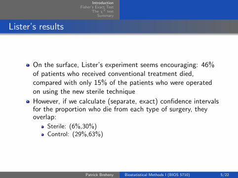
On the surface, Lister’s experiment seems encouraging: 46%of patients who received conventional treatment died,compared with only 15% of the patients who were operatedon using the new sterile technique
However, if we calculate (separate, exact) confidence intervalsfor the proportion who die from each type of surgery, theyoverlap:
Sterile: (6%,30%)Control: (29%,63%)
Patrick Breheny Biostatistical Methods I (BIOS 5710) 5/22
IntroductionFisher’s Exact Test
The χ2 testSummary
Lister experiment with balls and urns
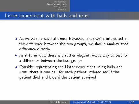
As we’ve said several times, however, since we’re interested inthe difference between the two groups, we should analyze thatdifference directly
As it turns out, there is a rather elegant, exact way to test fora difference between the two groups
Consider representing the Lister experiment using balls andurns: there is one ball for each patient, colored red if thepatient died and blue if the patient survived
Patrick Breheny Biostatistical Methods I (BIOS 5710) 6/22
IntroductionFisher’s Exact Test
The χ2 testSummary
Lister experiment with balls and urns (cont’d)
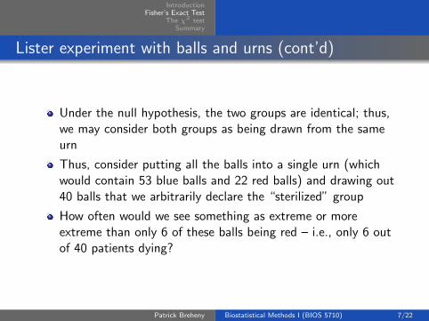
Under the null hypothesis, the two groups are identical; thus,we may consider both groups as being drawn from the sameurn
Thus, consider putting all the balls into a single urn (whichwould contain 53 blue balls and 22 red balls) and drawing out40 balls that we arbitrarily declare the “sterilized” group
How often would we see something as extreme or moreextreme than only 6 of these balls being red – i.e., only 6 outof 40 patients dying?
Patrick Breheny Biostatistical Methods I (BIOS 5710) 7/22

IntroductionFisher’s Exact Test
The χ2 testSummary
Calculating the p-value for Lister’s data
The probability of drawing 6 red balls is(5334
)(226
)(7540
) = 0.003
There are several results as extreme (improbable) or moreextreme than this, such as drawing 5 red balls (probability0.0006) or drawing 18 red balls (probability 0.001)
Adding up all such probabilities, we obtain p = 0.005; this isstrong evidence that sterile surgery reduces the probability ofdeath
Patrick Breheny Biostatistical Methods I (BIOS 5710) 8/22
IntroductionFisher’s Exact Test
The χ2 testSummary
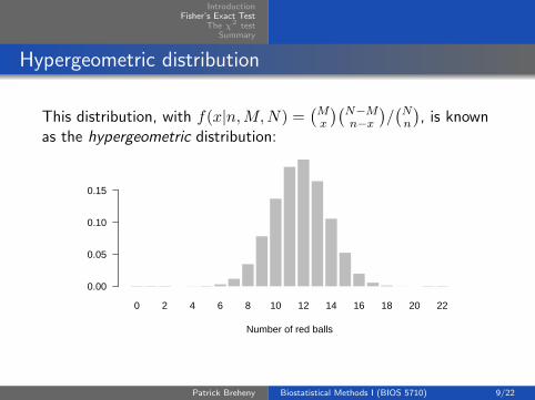
Hypergeometric distribution
This distribution, with f(x|n,M,N) =(Mx
)(N−Mn−x
)/(Nn
), is known
as the hypergeometric distribution:
0 2 4 6 8 10 12 14 16 18 20 22
Number of red balls
0.00
0.05
0.10
0.15
Patrick Breheny Biostatistical Methods I (BIOS 5710) 9/22
IntroductionFisher’s Exact Test
The χ2 testSummary
Fisher’s exact test
This approach to testing association in a 2x2 table is calledFisher’s exact test, after R.A. Fisher
The test may seem somewhat strange in the sense that we aretreating the number of patients who survived/died as fixedwhen we calculate our probability, even though of course it istruly random
Fisher’s rationale was that conditioning on the total numberof successes was justified by the fact that we are testing thedifference between the two groups, and the total number ofsuccesses contains no information about that difference(Fisher called such a statistic “ancillary”)
This was a novel idea in Fisher’s day, but the idea ofconditioning on ancillary statistics has since become a widelyaccepted approach to inference
Patrick Breheny Biostatistical Methods I (BIOS 5710) 10/22

IntroductionFisher’s Exact Test
The χ2 testSummary
The χ2 test
Fisher’s exact test involves a fair amount of calculation; whatdid people do before computational resources were soabundant?
As you can imagine from looking at the hypergeometricdistribution, it is possible to approach this problem using thenormal distribution to obtain approximate results
Indeed, even before Fisher, another famous statistician (KarlPearson) invented an approximate test for categorical data
Pearson’s invention, the χ2-test, is one of the earliest (1900)and still most widely used statistical tests
Patrick Breheny Biostatistical Methods I (BIOS 5710) 11/22
IntroductionFisher’s Exact Test
The χ2 testSummary
The χ2 distribution and hypothesis testing
As we’ve seen several times in the course, z-tests have thegeneral pattern: random variable minus its expected valuedivided by the standard error, which we take to beapproximately normal
Squaring this quantity, we have
(O − E)2
Var(O)∼ χ2
1,
where O is the observed value of the random variable and Eis its expected value
Note that this test statistic is naturally two-sided, in that both“left” and “right” extremes of the original z-test translateinto large values of the χ2 test statistic
Patrick Breheny Biostatistical Methods I (BIOS 5710) 12/22

IntroductionFisher’s Exact Test
The χ2 testSummary
The motivation behind a χ2-test
So essentially, the χ2 test is simply the squared version of thez-test
However, working with a squared quantity lends itselfnaturally to combining discrepancies between observed andexpected over all cells in a table
By adding up the (O − E)2/Var(O) values over each cell in atable, we obtain a total measure of disagreement between theactual counts and the counts we would expect under the nullhypothesis
Patrick Breheny Biostatistical Methods I (BIOS 5710) 13/22

IntroductionFisher’s Exact Test
The χ2 testSummary
The χ2-statistic
Letting the subscript i denote the cells of the table, we havethe test statistic
χ2 =∑i
(Oi − Ei)2
Ei,
where Oi and Ei are the observed and expected number oftimes category i occurs/should occurYou may be wondering about the denominator – why have wereplaced Var(O) with E?This can be justified a few ways, the simplest being that for aPoisson random variable (often used to model counts),Var(x) = E(X); we’ll discuss the Poisson distribution ingreater depth next weekIntuitively, however, it should make sense that as E increases,so does its variability
Patrick Breheny Biostatistical Methods I (BIOS 5710) 14/22

IntroductionFisher’s Exact Test
The χ2 testSummary
Distribution under the null
So we’ve defined our test statistic and it seems as though itshould follow some sort of a χ2 distribution (being the sum ofsquared standard normals)
However, the cells are obviously not independent, so perhapsthe test statistic doesn’t follow a χ2
4 distribution
It turns out to (approximately) follow a χ21 distribution,
although this is not an obvious fact – Pearson himself thoughtit followed a χ2
3 distribution, and was rather hostile to Fisher’s(1922) correction of his original χ2 derivation, and the twofeuded bitterly for many years
Patrick Breheny Biostatistical Methods I (BIOS 5710) 15/22

IntroductionFisher’s Exact Test
The χ2 testSummary
The χ2-test: Lister’s experiment
Let’s use the χ2-test to determine how unlikely Lister’s resultswould have been if sterile technique had no impact on fatalcomplications from surgery
First, let’s create a table of expected counts based on the nullhypothesis
In the experiment, ignoring group affiliation, 22 out of 75patients died; thus, under the null, we would expect22/75 = 29.3% of the patients in each group to die:
SurvivedYes No
Sterile 28.3 11.7Control 24.7 10.3
Patrick Breheny Biostatistical Methods I (BIOS 5710) 16/22

IntroductionFisher’s Exact Test
The χ2 testSummary
The χ2-test: Lister’s experiment (cont’d)
#2 Calculate the χ2-statistic:
χ2 =(34− 28.3)2
28.3+
(6− 11.7)2
11.7
+(19− 24.7)2
24.7+
(16− 10.3)2
10.3= 8.50
#3 The area to the right of 8.50 is 1− Fχ21(8.50) = .004
There is only a 0.4% probability of seeing such a largeassociation by chance alone; again, compelling evidence thatsterile surgical technique saves lives
Patrick Breheny Biostatistical Methods I (BIOS 5710) 17/22

IntroductionFisher’s Exact Test
The χ2 testSummary
Fisher’s exact test and the χ2-test
Both Fisher’s exact test and the χ2-test address the same nullhypothesis, so it is reassuring that we obtain virtually identicalresults for the Lister experiment (p = 0.005 vs. p = 0.004)
This is often the case for 2x2 tables: the results from Fisher’sexact test and the approximate χ2-test are typically in closeagreement
However, when there are many cells with small Ei numbers,the two can yield very different results
This is particularly problematic in larger tables
Patrick Breheny Biostatistical Methods I (BIOS 5710) 18/22

IntroductionFisher’s Exact Test
The χ2 testSummary
I × J tables
The ideas of Fisher’s exact test and the χ2 test may be readilyextended to larger tables with an arbitrary number of rows Iand columns J
For Fisher’s exact test, we can still represent the experimentusing balls and urns and calculate table probabilities, althoughthe result no longer follows a simple hypergeometricdistribution
For the χ2 test, the test statistic is exactly the same (justsumming over more cells), and follows a χ2
(I−1)(J−1)distribution under the null hypothesis
Patrick Breheny Biostatistical Methods I (BIOS 5710) 19/22

IntroductionFisher’s Exact Test
The χ2 testSummary
Example: Frequency of wearing gloves outside the lab
Some 4-year Master’s Other Prof.College Degree Degree Ph.D. Degree
Sometimes 1 0 0 0 0Rarely 1 3 5 15 0Never 1 17 13 38 3
Fisher’s Exact Test: p = .12
χ2-test: p = .00003
Patrick Breheny Biostatistical Methods I (BIOS 5710) 20/22

IntroductionFisher’s Exact Test
The χ2 testSummary
Fisher’s exact test vs. the χ2-test
How should you decide to use one versus the other?
As in the case of one-sample data, with modern computersthere is little reason to settle for the approximate answer whenthe exact answer can be calculated in a fraction of a second
Nevertheless, χ2-tests are still widely used, largely due toinertia and tradition, but also because the two generallyprovide very similar results, especially for 2x2 tables
It is important to be aware, however, that the χ2-test can bewildly incorrect when some cells have small Ei values – as arule of thumb, this starts to become a problem when Ei < 5,but becomes extreme when Ei < 1
Patrick Breheny Biostatistical Methods I (BIOS 5710) 21/22

IntroductionFisher’s Exact Test
The χ2 testSummary
Summary
Contingency tables cross-classify observations in a studyaccording to group and outcome
The null hypothesis that group membership is independent ofthe outcome can be tested using two common approaches:
Fisher’s exact test is an exact test based on conditioning onthe total number of successes and failuresThe χ2 test is an approximate (large-sample/central limittheorem) test based on summing up normalized differences inobserved and expected counts over all cells in a table
The two generally yield similar answers, although will start todiverge when the expected cell counts drop below ≈ 5
Patrick Breheny Biostatistical Methods I (BIOS 5710) 22/22


![Asymmetries in the representation of categorical ... · Asymmetries in the representation of categorical phonotactics* Gillian Gallagher, New York University ... e.g., *[kap’a],](https://static.fdocument.pub/doc/165x107/5aea2e3d7f8b9ad73f8cd422/asymmetries-in-the-representation-of-categorical-in-the-representation-of-categorical.jpg)