Transformations and the Graphics Pipeline - 南京航空航...

C H A P T E R 4

Transformations and theGraphics Pipeline

Prerequisites: Chapters 2 and 3 in [AgoM05]. Chapter 20 for Section 4.14.

4.1 Introduction

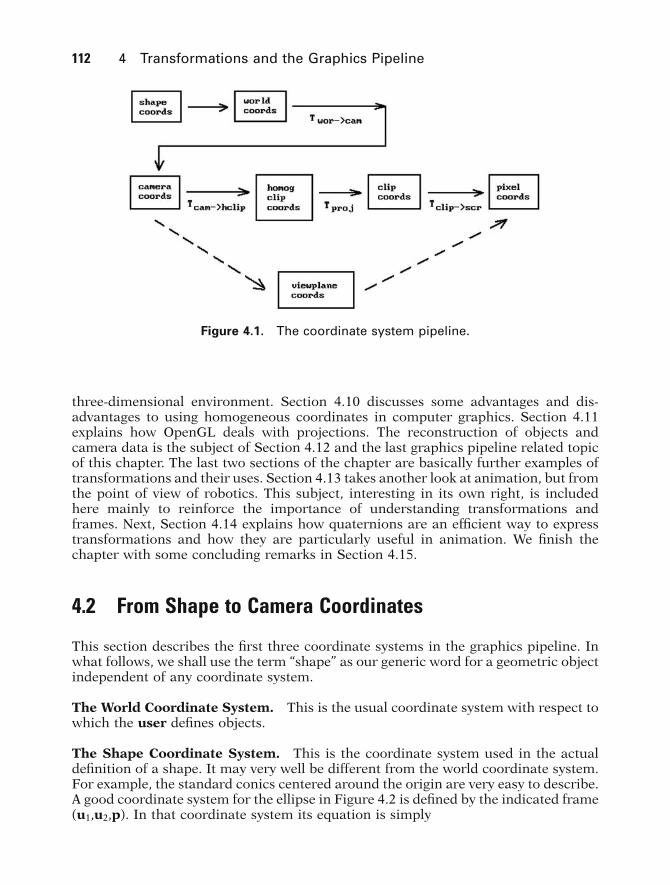
In this chapter we combine properties of motions, homogeneous coordinates, pro-jective transformations, and clipping to describe the mathematics behind the three-dimensional computer graphics transformation pipeline. With this knowledge one willthen know all there is to know about how to display three-dimensional points on ascreen and subsequent chapters will not have to worry about this issue and can con-centrate on geometry and rendering issues. Figure 4.1 shows the main coordinatesystems that one needs to deal with in graphics and how they fit into the pipeline. Thesolid line path includes clipping, the dashed line path does not.

Because the concept of a coordinate system is central to this chapter, it is worthmaking sure that there is no confusion here. The term “coordinate system” for Rn

means nothing but a “frame” in Rn, that is, a tuple consisting of an orthonormal basisof vectors together with a point that corresponds to the “origin” of the coordinatesystem. The terms will be used interchangeably. In this context one thinks of Rn purelyas a set of “points” with no reference to coordinates. Given one of these abstract pointsp, one can talk about the coordinates of p with respect to one coordinate system orother. If p = (x,y,z) Œ R3, then x, y, and z are of course just the coordinates of p withrespect to the standard coordinate system or frame (e1,e2,e3,0).

Describing the coordinate systems and maps shown in Figure 4.1 and dealing withthat transformation pipeline in general occupies Sections 4.2–4.7. Much of the dis-cussion is heavily influenced by Blinn’s excellent articles [Blin88b,91a–c,92]. Theymake highly recommended reading. Section 4.8 describes what is involved in creat-ing stereo views. Section 4.9 discusses parallel projections and how one can use thespecial case of orthographic projections to implement two-dimensional graphics in a

GOS04 5/5/2005 6:18 PM 11

three-dimensional environment. Section 4.10 discusses some advantages and dis-advantages to using homogeneous coordinates in computer graphics. Section 4.11explains how OpenGL deals with projections. The reconstruction of objects andcamera data is the subject of Section 4.12 and the last graphics pipeline related topicof this chapter. The last two sections of the chapter are basically further examples oftransformations and their uses. Section 4.13 takes another look at animation, but fromthe point of view of robotics. This subject, interesting in its own right, is includedhere mainly to reinforce the importance of understanding transformations andframes. Next, Section 4.14 explains how quaternions are an efficient way to expresstransformations and how they are particularly useful in animation. We finish thechapter with some concluding remarks in Section 4.15.

4.2 From Shape to Camera Coordinates

This section describes the first three coordinate systems in the graphics pipeline. Inwhat follows, we shall use the term “shape” as our generic word for a geometric objectindependent of any coordinate system.

The World Coordinate System. This is the usual coordinate system with respect towhich the user defines objects.

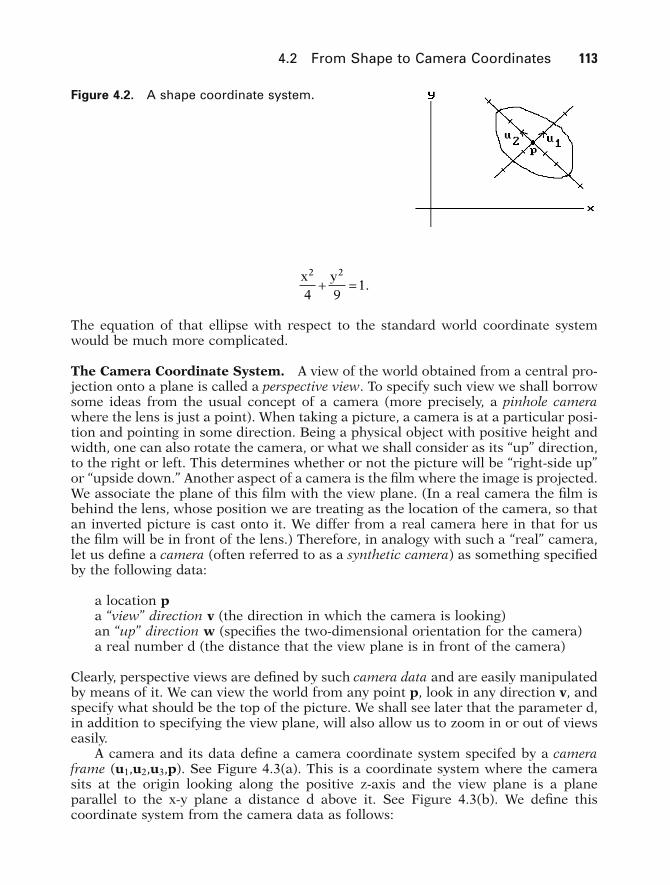
The Shape Coordinate System. This is the coordinate system used in the actualdefinition of a shape. It may very well be different from the world coordinate system.For example, the standard conics centered around the origin are very easy to describe.A good coordinate system for the ellipse in Figure 4.2 is defined by the indicated frame(u1,u2,p). In that coordinate system its equation is simply

112 4 Transformations and the Graphics Pipeline

Figure 4.1. The coordinate system pipeline.

GOS04 5/5/2005 6:18 PM Page 112

4.2 From Shape to Camera Coordinates 113

Figure 4.2. A shape coordinate system.

The equation of that ellipse with respect to the standard world coordinate systemwould be much more complicated.

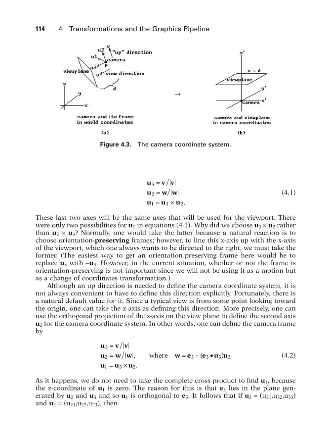
The Camera Coordinate System. A view of the world obtained from a central pro-jection onto a plane is called a perspective view. To specify such view we shall borrowsome ideas from the usual concept of a camera (more precisely, a pinhole camerawhere the lens is just a point). When taking a picture, a camera is at a particular posi-tion and pointing in some direction. Being a physical object with positive height andwidth, one can also rotate the camera, or what we shall consider as its “up” direction,to the right or left. This determines whether or not the picture will be “right-side up”or “upside down.” Another aspect of a camera is the film where the image is projected.We associate the plane of this film with the view plane. (In a real camera the film isbehind the lens, whose position we are treating as the location of the camera, so thatan inverted picture is cast onto it. We differ from a real camera here in that for usthe film will be in front of the lens.) Therefore, in analogy with such a “real” camera,let us define a camera (often referred to as a synthetic camera) as something specifiedby the following data:

a location pa “view” direction v (the direction in which the camera is looking)an “up” direction w (specifies the two-dimensional orientation for the camera)a real number d (the distance that the view plane is in front of the camera)

Clearly, perspective views are defined by such camera data and are easily manipulatedby means of it. We can view the world from any point p, look in any direction v, andspecify what should be the top of the picture. We shall see later that the parameter d,in addition to specifying the view plane, will also allow us to zoom in or out of viewseasily.

A camera and its data define a camera coordinate system specifed by a cameraframe (u1,u2,u3,p). See Figure 4.3(a). This is a coordinate system where the camerasits at the origin looking along the positive z-axis and the view plane is a plane parallel to the x-y plane a distance d above it. See Figure 4.3(b). We define this coordinate system from the camera data as follows:

x y2 2

4 91+ = .

GOS04 5/5/2005 6:18 PM Page 113

(4.1)

These last two axes will be the same axes that will be used for the viewport. Therewere only two possibilities for u1 in equations (4.1). Why did we choose u3 ¥ u2 ratherthan u2 ¥ u3? Normally, one would take the latter because a natural reaction is tochoose orientation-preserving frames; however, to line this x-axis up with the x-axisof the viewport, which one always wants to be directed to the right, we must take theformer. (The easiest way to get an orientation-preserving frame here would be toreplace u3 with -u3. However, in the current situation, whether or not the frame isorientation-preserving is not important since we will not be using it as a motion butas a change of coordinates transformation.)

Although an up direction is needed to define the camera coordinate system, it isnot always convenient to have to define this direction explicitly. Fortunately, there isa natural default value for it. Since a typical view is from some point looking towardthe origin, one can take the z-axis as defining this direction. More precisely, one canuse the orthogonal projection of the z-axis on the view plane to define the second axisu2 for the camera coordinate system. In other words, one can define the camera frameby

(4.2)

As it happens, we do not need to take the complete cross product to find u1, becausethe z-coordinate of u1 is zero. The reason for this is that e3 lies in the plane gen-erated by u2 and u3 and so u1 is orthogonal to e3. It follows that if u3 = (u31,u32,u33)and u2 = (u21,u22,u23), then

u v v

u w w w e e u u

u u u

3

2 3 3 3 3

1 3 2

== = - ∑( )= ¥

,

.

where

u v v

u w w

u u u

3

2

1 3 2

=== ¥ .


ÆÆ

Figure 4.3. The camera coordinate system.

GOS04 5/5/2005 6:18 PM Page 114

It is also easy to show that u1 is a positive scalar multiple of (u32,-u31,0) (Exercise4.2.1), so that

(4.3)

Although this characterization of u1 is useful and easier to remember than the crossproduct, it is not as efficient because it involves taking a square root.

Note that there is one case where our construction does not work, namely, whenthe camera is looking in a direction parallel to the z-axis. In that case the orthogonalprojection of the z-axis on the view plane is the zero vector. In this case one can arbi-trarily use the orthogonal projection of the y-axis on the view plane to define u2. For-tunately, in practice it is rare that one runs into this case. If one does, what will happenis that the picture on the screen will most likely suddenly flip around to some unex-pected orientation. Such a thing would not happen with a real camera. One canprevent it by keeping track of the frames as the camera moves. Then when the cameramoves onto the z-axis one could define the new frame from the frames at previousnearby positions using continuity. This involves a lot of extra work though which isusually not worth it. Of course, if it is important to avoid these albeit rare occurrencesthen one can do the extra work or require that the user specify the desired up direc-tion explicitly.

Finally, given the frame F = (u1,u2,u3,p) for the camera, then the world-to-cameracoordinate transformation TworÆcam in Figure 4.1 is the map

(4.4)

where M is the 3 ¥ 3 matrix that has the vectors ui as its columns.We begin with a two-dimensional example.

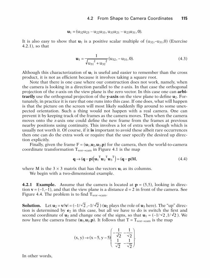
4.2.1 Example. Assume that the camera is located at p = (5,5), looking in direc-tion v = (-1,-1), and that the view plane is a distance d = 2 in front of the camera. SeeFigure 4.4. The problem is to find TworÆcam.

Solution. Let u2 = v/|v| = (-1/ ,-1/ ) (u2 plays the role of u3 here). The “up” direc-tion is determined by e2 in this case, but all we have to do is switch the first andsecond coordinate of u2 and change one of the signs, so that u1 = (-1/ ,1/ ). Wenow have the camera frame (u1,u2,p). It follows that T = TworÆcam is the map

In other words,

x y x y, , .( ) Æ - -( )- -

-

Ê

Ë

ÁÁÁ

ˆ

¯

˜˜˜

5 5

1

21

2

1

21

2

22

22

q q p u u u q pÆ -( )( ) = -( )1 2 3T T T

M,

u1

312

322 32 31

10=

+-( )

u uu u, , .

u1 32 23 22 33 33 21 23 31 0= - -( )u u u u u u u u, , .

4.2 From Shape to Camera Coordinates 115

GOS04 5/5/2005 6:18 PM Page 115

As a quick check we compute T(5,5) = (0,0) and T(5 - ,5 - ) = (0,2), which clearlyare the correct values.

Next, we work through a three-dimensional example.

4.2.2 Example. Assume that the camera is located at p = (5,1,2), looking in direc-tion v = (-1,-2,-1), and that the view plane is a distance d = 3 in front of the camera.The problem again is to find TworÆcam.

Solution. Using equations (4.2) we get

It follows that

T x x y

y x y z

z x y z

wor camÆ ¢ =-

-( ) + -( )

¢ =-

-( ) +-

-( ) + -( )

¢ =-

-( ) +-

-( ) +-

-( )

:

.

2

55

1

51

1

305

2

301

5

302

1

65

2

61

1

62

u

u w w w

u u u

3

2

1 3 2

1

61 2 1

1

301 2 5

16

1 2 5

1

52 1 0

= - - -( )

= = - -( ) = - -( )

= ¥ = -( )

, ,

, , , , ,

, , .

where

22

T x x y x y

y x y x y

wor camÆ ¢ = - -( ) + -( ) = - +

¢ = - -( ) - -( ) = - - +

:1

25

1

25

1

2

1

21

25

1

25

1

2

1

25 2


Figure 4.4. Transforming from world tocamera coordinates.

GOS04 5/5/2005 6:18 PM Page 116

Note in the two examples how the frame that defines the camera coordinatesystem also defines the transformation from world coordinates to camera coordinatesand conversely. The frame is the whole key to camera coordinates and look how simpleit was to define this frame!

The View Plane Coordinate System. The origin of this coordinate system is thepoint in the view plane a distance d directly in front of the camera and the x- and y-axis are the same as those of the camera coordinate system. More precisely, if(u1,u2,u3,p) is the camera coordinate system, then (u1,u2,p+du3) is the view planecoordinate system.

4.3 Vanishing Points

If there is no clipping, then after one has the camera coordinates of a point, the nextproblem is to project to the view plane z = d. The central projection p of R3 from theorigin to this plane is easy to compute. Using similarity of triangles, we get

(4.5)

Let us see what happens when lines are projected to the view plane. Consider a line through a point p0 = (x0,y0,z0), with direction vector v = (a,b,c), and parameterization

(4.6)

This line is projected by p to a curve p¢(t) = (x¢(t),y¢(t),d) in the view plane, where

(4.7)

It is easy to check that the slope of the line segment from p¢(t1) to p¢(t2) is

which is independent of t1 and t2. This shows that the curve p¢(t) has constant slopeand reconfirms the fact that central projections project lines into lines (but not necessarily onto).

Next, let us see what happens to p¢(t) as t goes to infinity. Assume that c π 0. Then,using equation (4.7), we get that

(4.8)

This limit point depends only on the direction vector v of the original line. What thismeans is that all lines with the same direction vector, that is, all lines parallel to the

lim , ,t

x t y t da c db cÆ•

¢( ) ¢( )( ) = ( )

¢( ) - ¢( )¢( ) - ¢( ) =

--

y t y tx t x t

y c bzx c az

2 1

2 1

0 0

0 0,

¢( ) =++

¢( ) =++

x t dx atz ct

and y t dy btz ct

0

0

0

0;

p t x t y t z t t( ) = ( ) ( ) ( )( ) = +, , .p v0

p x y z x y d d x z d y z d, , , , , , .( ) = ¢ ¢( ) = ( )

4.3 Vanishing Points 117

GOS04 5/5/2005 6:18 PM Page 117

original line, will project to lines that intersect in a point. If c = 0, then one can checkthat nothing special happens and parallel lines project into parallel lines.

In the context of the world-to-view plane transformation with respect to a givencamera, what we have shown is that lines in the world project into lines in the viewplane. Furthermore, the projection of some lines gives rise to certain special pointsin the view plane. Specifically, let L be a line in the world and let equation (4.6) be aparameterization for L in camera coordinates. We use the notation in the discussionabove.

Definition. If the point in the view plane of the camera that corresponds to the pointon the right hand side of equation (4.8) exists, then it is called the vanishing point forthe line L with respect to the given camera or view.

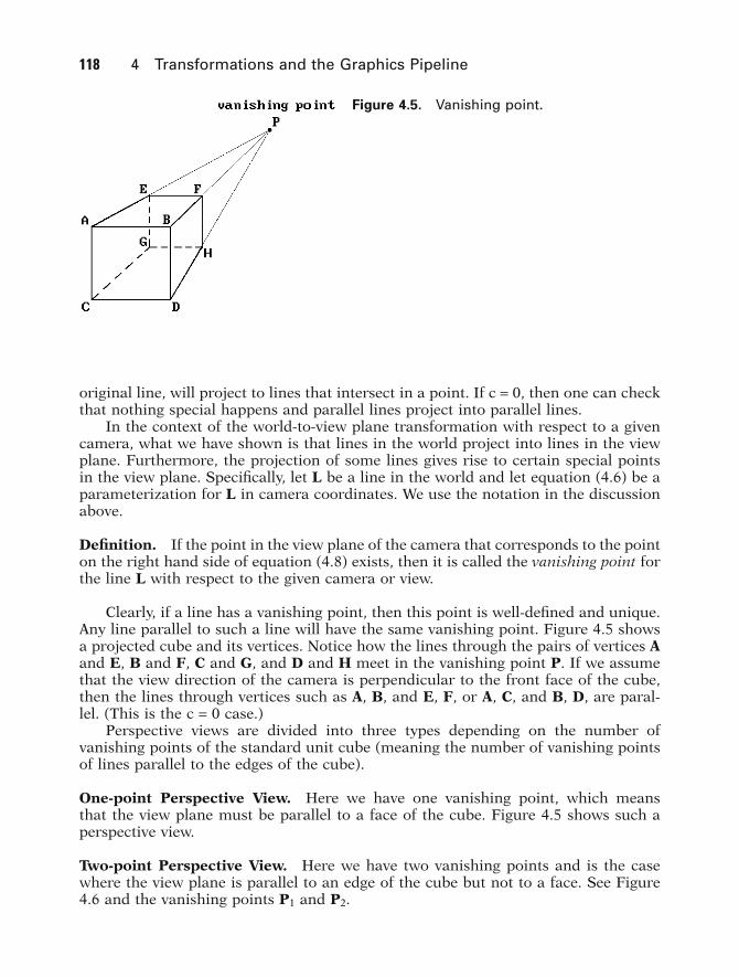
Clearly, if a line has a vanishing point, then this point is well-defined and unique.Any line parallel to such a line will have the same vanishing point. Figure 4.5 showsa projected cube and its vertices. Notice how the lines through the pairs of vertices Aand E, B and F, C and G, and D and H meet in the vanishing point P. If we assumethat the view direction of the camera is perpendicular to the front face of the cube,then the lines through vertices such as A, B, and E, F, or A, C, and B, D, are paral-lel. (This is the c = 0 case.)

Perspective views are divided into three types depending on the number of vanishing points of the standard unit cube (meaning the number of vanishing pointsof lines parallel to the edges of the cube).

One-point Perspective View. Here we have one vanishing point, which means that the view plane must be parallel to a face of the cube. Figure 4.5 shows such aperspective view.

Two-point Perspective View. Here we have two vanishing points and is the casewhere the view plane is parallel to an edge of the cube but not to a face. See Figure4.6 and the vanishing points P1 and P2.


Figure 4.5. Vanishing point.

GOS04 5/5/2005 6:18 PM Page 118

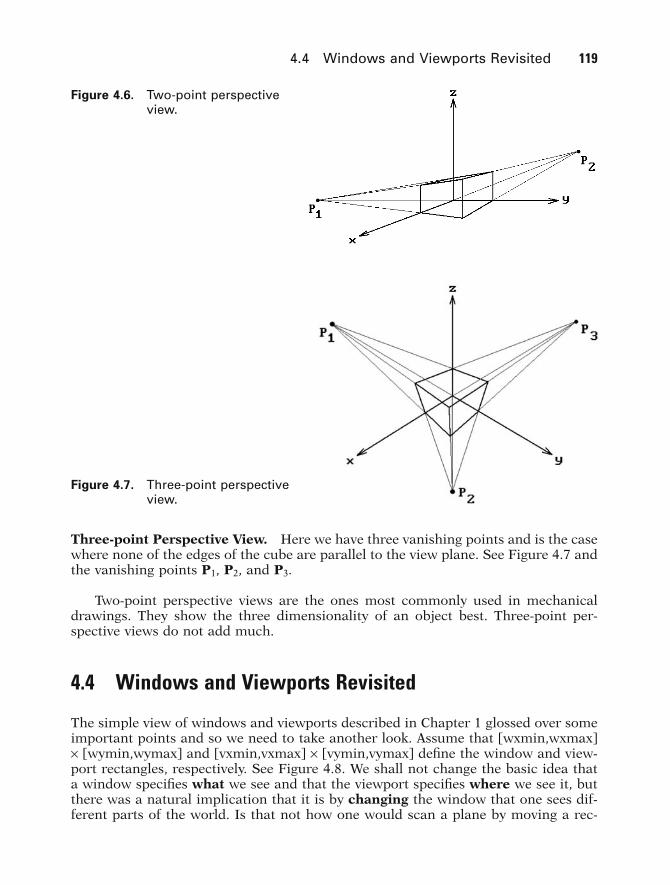
Three-point Perspective View. Here we have three vanishing points and is the casewhere none of the edges of the cube are parallel to the view plane. See Figure 4.7 andthe vanishing points P1, P2, and P3.

Two-point perspective views are the ones most commonly used in mechanicaldrawings. They show the three dimensionality of an object best. Three-point per-spective views do not add much.

4.4 Windows and Viewports Revisited

The simple view of windows and viewports described in Chapter 1 glossed over someimportant points and so we need to take another look. Assume that [wxmin,wxmax]¥ [wymin,wymax] and [vxmin,vxmax] ¥ [vymin,vymax] define the window and view-port rectangles, respectively. See Figure 4.8. We shall not change the basic idea thata window specifies what we see and that the viewport specifies where we see it, butthere was a natural implication that it is by changing the window that one sees dif-ferent parts of the world. Is that not how one would scan a plane by moving a rec-

4.4 Windows and Viewports Revisited 119

Figure 4.6. Two-point perspectiveview.

Figure 4.7. Three-point perspectiveview.

GOS04 5/5/2005 6:18 PM Page 119

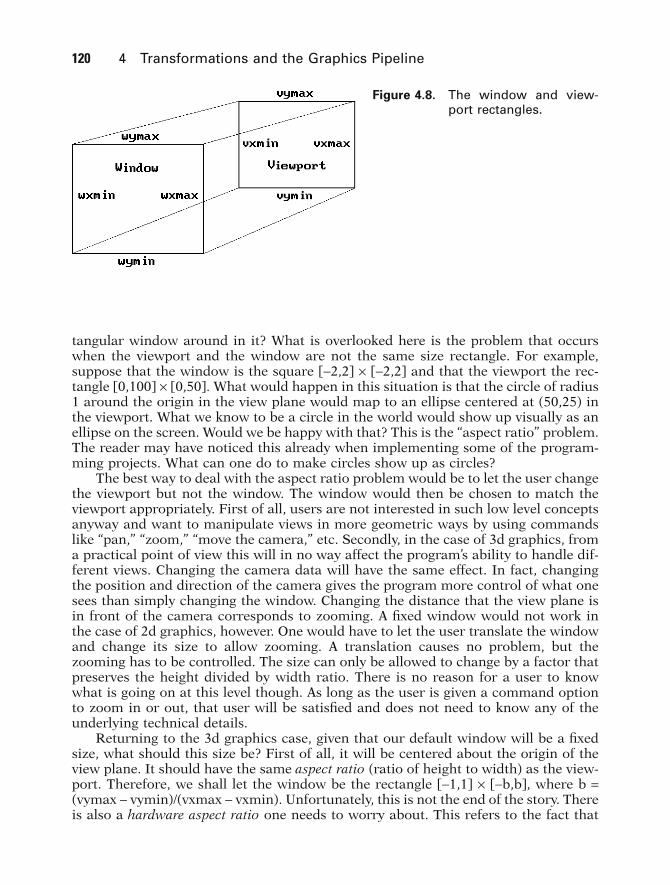
tangular window around in it? What is overlooked here is the problem that occurswhen the viewport and the window are not the same size rectangle. For example,suppose that the window is the square [-2,2] ¥ [-2,2] and that the viewport the rec-tangle [0,100] ¥ [0,50]. What would happen in this situation is that the circle of radius1 around the origin in the view plane would map to an ellipse centered at (50,25) inthe viewport. What we know to be a circle in the world would show up visually as anellipse on the screen. Would we be happy with that? This is the “aspect ratio” problem.The reader may have noticed this already when implementing some of the program-ming projects. What can one do to make circles show up as circles?

The best way to deal with the aspect ratio problem would be to let the user changethe viewport but not the window. The window would then be chosen to match theviewport appropriately. First of all, users are not interested in such low level conceptsanyway and want to manipulate views in more geometric ways by using commandslike “pan,” “zoom,” “move the camera,” etc. Secondly, in the case of 3d graphics, froma practical point of view this will in no way affect the program’s ability to handle dif-ferent views. Changing the camera data will have the same effect. In fact, changingthe position and direction of the camera gives the program more control of what onesees than simply changing the window. Changing the distance that the view plane isin front of the camera corresponds to zooming. A fixed window would not work inthe case of 2d graphics, however. One would have to let the user translate the windowand change its size to allow zooming. A translation causes no problem, but thezooming has to be controlled. The size can only be allowed to change by a factor thatpreserves the height divided by width ratio. There is no reason for a user to knowwhat is going on at this level though. As long as the user is given a command optionto zoom in or out, that user will be satisfied and does not need to know any of theunderlying technical details.

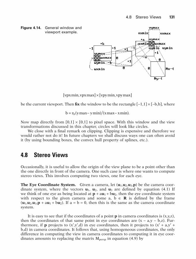
Returning to the 3d graphics case, given that our default window will be a fixedsize, what should this size be? First of all, it will be centered about the origin of theview plane. It should have the same aspect ratio (ratio of height to width) as the view-port. Therefore, we shall let the window be the rectangle [-1,1] ¥ [-b,b], where b =(vymax - vymin)/(vxmax - vxmin). Unfortunately, this is not the end of the story. Thereis also a hardware aspect ratio one needs to worry about. This refers to the fact that


Figure 4.8. The window and view-port rectangles.

GOS04 5/5/2005 6:18 PM Page 120

the dots of the electron beam for the CRT may not be “square.” The hardware ratiois usually expressed in the form a = ya/xa with the operating system supplying thevalues xa and ya. In Microsoft Windows, one gets these values via the calls

where hdc is a “device context” and ASPECTX and ASPECTY are system-defined constants.

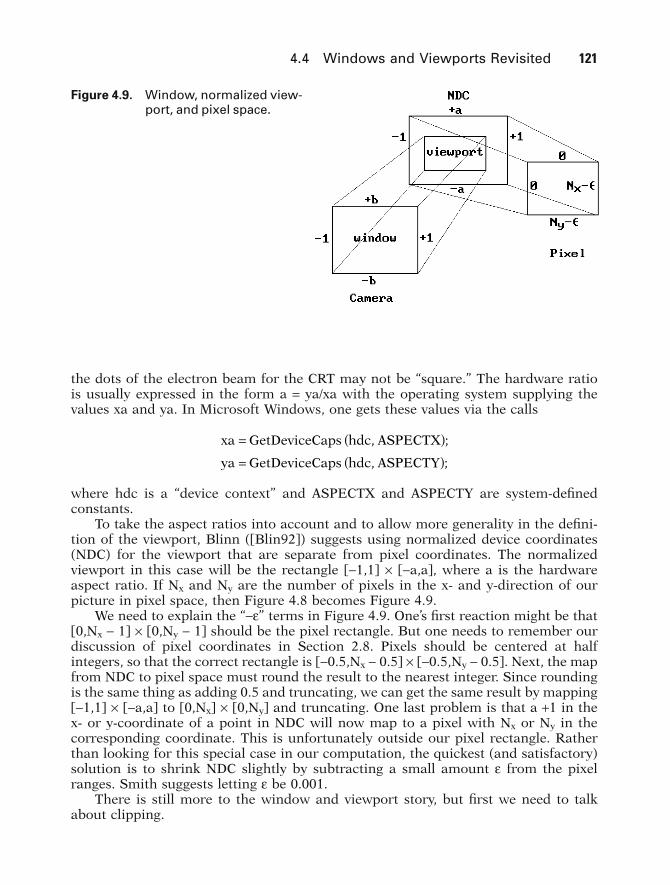
To take the aspect ratios into account and to allow more generality in the defini-tion of the viewport, Blinn ([Blin92]) suggests using normalized device coordinates(NDC) for the viewport that are separate from pixel coordinates. The normalizedviewport in this case will be the rectangle [-1,1] ¥ [-a,a], where a is the hardwareaspect ratio. If Nx and Ny are the number of pixels in the x- and y-direction of ourpicture in pixel space, then Figure 4.8 becomes Figure 4.9.

We need to explain the “-e” terms in Figure 4.9. One’s first reaction might be that[0,Nx - 1] ¥ [0,Ny - 1] should be the pixel rectangle. But one needs to remember ourdiscussion of pixel coordinates in Section 2.8. Pixels should be centered at half integers, so that the correct rectangle is [-0.5,Nx - 0.5] ¥ [-0.5,Ny - 0.5]. Next, the mapfrom NDC to pixel space must round the result to the nearest integer. Since roundingis the same thing as adding 0.5 and truncating, we can get the same result by mapping[-1,1] ¥ [-a,a] to [0,Nx] ¥ [0,Ny] and truncating. One last problem is that a +1 in thex- or y-coordinate of a point in NDC will now map to a pixel with Nx or Ny in the corresponding coordinate. This is unfortunately outside our pixel rectangle. Ratherthan looking for this special case in our computation, the quickest (and satisfactory)solution is to shrink NDC slightly by subtracting a small amount e from the pixelranges. Smith suggests letting e be 0.001.

There is still more to the window and viewport story, but first we need to talkabout clipping.

xa GetDeviceCaps hdc ASPECTX

ya GetDeviceCaps hdc ASPECTY

= ( )= ( )

, ;

, ;

4.4 Windows and Viewports Revisited 121

Figure 4.9. Window, normalized view-port, and pixel space.

GOS04 5/5/2005 6:18 PM Page 121

4.5 The Clip Coordinate System

Once one has transformed objects into camera coordinates, our next problem is toclip points in the camera coordinate system to the truncated pyramid defined by the near and far clipping planes and the window. One could do this directly, but weprefer to transform into a coordinate system, called the clip coordinate system or clipspace, where the clipping volume is the unit cube [0,1] ¥ [0,1] ¥ [0,1]. We denote thetransformation that does this by TcamÆclip. There are two reasons for using this transformation:

(1) It is clearly simpler to clip against the unit cube.(2) The clipping algorithm becomes independent of boundary dimensions.

Actually, rather than using these coordinates we shall use the associated homogeneouscoordinates. The latter define what we shall call the homogeneous clip coordinatesystem or homogeneous clip space. Using homogeneous coordinates will enable us todescribe maps via matrices and we will also not have to worry about any divisions byzero on our way to the clip stage. The map TcamÆhclip in Figure 4.1 refers to thiscamera-to-homogeneous-clip coordinates transformation. Let ThcamÆhclip denote thecorresponding homogeneous-camera-to-homogeneous-clip coordinates transforma-tion. Figure 4.10 shows the relationships between all these maps. The map Tproj is the standard projection from homogeneous to Euclidean coordinates.

Assume that the view plane and near and far clipping planes are a distance d, dn,and df in front of the camera, respectively. To describe TcamÆhclip, it will suffice todescribe ThcamÆhclip.

First of all, translate the camera to (0,0,-d). This translation is represented by thehomogeneous matrix

M

d

tr =

-

Ê

Ë

ÁÁÁÁ

ˆ

¯

˜˜˜̃

1 0 0 0

0 1 0 0

0 0 1 0

0 0 1

.


Figure 4.10. The camera-to-clipspace transformations.

GOS04 5/5/2005 6:18 PM 2

Next, apply the projective transformation with homogeneous matrix Mpersp, where

(4.9)

To see exactly what the map defined by Mpersp does geometrically, consider the linesax + z = -d and ax - z = d in the plane y = 0. Note that (x,y,z,w) Mpersp = (x,y,z,(z/d)+w).In particular,

This shows that the camera at (0,0,-d) has been mapped to “infinity” and the two lineshave been mapped to the lines x¢ = -d/a and x¢ = d/a, respectively, in the plane y = 0.See Figure 4.11. In general, lines through (0,0,-d) are mapped to vertical lines throughtheir intersection with the x-y plane. Furthermore, what was the central projectionfrom the point (0,0,-d) is now an orthogonal projection of R3 onto the x-y plane. Itfollows that the composition of Mtr and Mpersp maps the camera off to “infinity,” thenear clipping plane to z = d (1 - d/dn), and the far clipping plane to z = d (1 - d/df).The perspective projection problem has been transformed into a simple orthographicprojection problem (we simply project (x,y,z) to (x,y,0)) with the clip volume now being

-[ ] ¥ -[ ] ¥ -( ) -( )[ ]1 1 1 1, , , .b b d d d d d df n

0 0 1 0 0 0

0 1 0 0 1

0 1 0 0

2

, , , , , ,

, , , , , , , , ,

, , , , , , , ,

-( ) = -( )

- -( ) = - - -ÊË

ˆ¯ = - - +Ê

ËÁˆ¯̃

- +( ) = - +ÊË

ˆ¯ =

d M d

x d ax M x d axaxd

dax

da

ddax

x d ax M x d axaxd

dax

da

d

persp

persp

persp --ÊËÁ

ˆ¯̃

dax

2

1, .

Md

persp =

Ê

Ë

ÁÁÁÁ

ˆ

¯

˜˜˜̃

1 0 0 0

0 1 0 0

0 0 1 1

0 0 0 1

.

4.5 The Clip Coordinate System 123

Figure 4.11. Mapping the camera to infinity.

GOS04 5/5/2005 6:18 PM Page 123

To get this new clip volume into the unit cube, we use the composite of the followingmaps: first, translate to

and then use the radial transformation which multiplies the x, y, and z-coordinatesby

respectively. If Mscale is the homogeneous matrix for the composite of these two maps,then

so that

(4.10)

is the matrix for the map ThcamÆhclip that we are after. It defines the transformationfrom homogeneous camera to homogeneous clip coordinates. By construction themap TcamÆclip sends the truncated view volume in camera coordinates into the unitcube [0,1] ¥ [0,1] ¥ [0,1] in clip space.

Note that the camera-to-clip-space transformation does not cost us anythingbecause it is computed only once and right away combined with the world-to-camera-space transformation so that points are only transformed once, not twice.

Finally, our camera-to-clip-space transformation maps three-dimensional pointsto three-dimensional points. In some cases, such as for wireframe displays, the z-coordinate is not needed and we could eliminate a few computations above. However,

M M M M d

d d

d

d d d dd d

d d d

hcam hclip tr persp scalef

f n

n f

f n

Æ = =

-( )

--( )

Ê

Ë

ÁÁÁÁÁÁÁÁ

ˆ

¯

˜˜˜˜˜˜˜˜

1

20 0 0

01

20 0

1

2

1

2

1

0 0 0

Md

d d

d d dd d dd d d

scalen f

f n

n f

f n

=

-( )

--( )

-( )

Ê

Ë

ÁÁÁÁÁÁÁÁ

ˆ

¯

˜˜˜˜˜˜˜˜

12

0 0 0

012

0 0

0 0 0

12

12

1

2

,

12

12 2

, , ,b

andd d

d d dn f

f n-( )

0 2 0 2 01 12, , , ,[ ] ¥ [ ] ¥ -Ê

Ëˆ¯

ÈÎÍ

˘˚̇

b dd dn f


GOS04 5/5/2005 6:18 PM Page 124

if we want to implement visible surface algorithms, then we need the z. Note that thetransformation is not a motion and will deform objects. However, and this is theimportant fact, it preserves relative z-distances from the camera and to determinethe visible surfaces we only care about relative and not absolute distances. More pre-cisely, let p1 and p2 be two points that lie along a ray in front of the camera and assumethat they map to p1¢ and p2¢, respectively, in clip space. If the z-coordinate of p1 isless than the z-coordinate of p2, then the z-coordinate of p1¢ will be less than the z-coordinate of p2¢. In other words, the “in front of” relation is preserved. To see this,let pi = (tix, tiy, tiz), 0 < t1 < t2, and pi¢ = (xi¢, yi¢, zi¢). It follows from (4.10) that

from which it is easy to show that t1 < t2 if and only if z1¢ < z2¢.

4.6 Clipping

In the last section we showed how to transform the clipping problem to a problem ofclipping against the unit cube in clip space. The actual clipping against the cube willbe done in homogeneous clip space using homogeneous coordinates (x,y,z,w). Theadvantage of homogeneous coordinates was already alluded to: every point of cameraspace is sent to a well-defined point here because values become undefined only whenwe try to map down to clip space by dividing by w, which may be zero.

Chapter 3 discussed general clipping algorithms for individual segments or wholepolygons. These have their place, but they are not geared to geometric modeling envi-ronments where one often wants to draw connected segments. We shall now describea very efficient clipping algorithm for such a setting that comes from [Blin91a]. It usesthe “best” parts of the Cohen-Sutherland, Cyrus-Beck, and Liang-Barsky algorithms.

In homogeneous coordinates halfplanes can be defined as a set of points that havea nonnegative dot product with a fixed vector. For example, the halfplane ax + by +cz + d ≥ 0, is defined by the vector (a,b,c,d) in homogeneous coordinates. Therefore,by lining up vectors appropriately, any convex region bounded by planes can bedefined as the set of points that have nonnegative dot products with a fixed finite setof vectors. In our case, we can use the following vectors for the six bounding planesx = 0, x = 1, y = 0, y = 1, z = 0, and z = 1 for the unit cube I3:

If p = (x,y,z,w), then let BCi = BCi(p) = p•Bi. We shall call the BCi the boundary coor-dinates of p. These coordinates are easy to compute:

BC x BC y BC z

BC w x BC w y BC w z

1 3 5

2 4 6

= = =

= - = - = -

, , ,

, , .

B B B

B B B

1 3 5

2 4 6

1 0 0 0 0 1 0 0 0 0 1 0

1 0 0 1 0 1 0 1 0 0 1 1

= ( ) = ( ) = ( )

= -( ) = -( ) = -( ), , , , , , , , , , , ,

, , , , , , , , , , , .

zdt z

dd di

n

i

f

f n

¢ = -ÊË

ˆ¯ -( )1

4.6 Clipping 125

GOS04 5/5/2005 6:18 PM Page 125

A point will be inside the clip volume if and only if all of its boundary coordinates arenonnegative. If the ith boundary coordinate of a point is nonnegative, then we shallcall the point i-inside; otherwise, it is i-out. Let BC = BC(p) = (BC1(p),BC2(p), . . . ,BC6(p)) denote the vector of boundary coordinates.

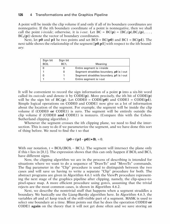
Next, let p0 and p1 be two points and set BC0 = BC(p0) and BC1 = BC(p1). Thenext table shows the relationship of the segment [p0,p1] with respect to the ith bound-ary:


Sign bit Sign bitBC0i BC1i Meaning

0 0 Entire segment is i-inside1 0 Segment straddles boundary, p0 is i-out0 1 Segment straddles boundary, p1 is i-out1 1 Entire segment is i-out

It will be convenient to record the sign information of a point p into a six-bit wordcalled its outcode and denote it by CODE(p). More precisely, the ith bit of CODE(p)will be the sign bit of BCi(p). Let CODE0 = CODE(p0) and CODE1 = CODE(p1).Simple logical operations on CODE0 and CODE1 now give us a lot of informationabout the location of the segment. For example, the segment will be inside the clipvolume if (CODE0 or CODE1) is zero. The segment will be entirely outside the clip volume if (CODE0 and CODE1) is nonzero. (Compare this with the Cohen-Sutherland clipping algorithm.)

Whenever the segment crosses the ith clipping plane, we need to find the inter-section. This is easy to do if we parameterize the segment, and we have done this sortof thing before. We need to find the t so that

With our notation, t = BC0i/(BC0i - BC1i). The segment will intersect the plane onlyif this t lies in [0,1]. The expression shows that this can only happen if BC0i and BC1ihave different signs.

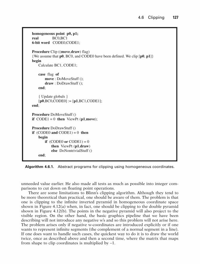
Now, the clipping algorithm we are in the process of describing is intended forsituations where we want to do a sequence of “DrawTo” and “MoveTo” commands.The flag parameter in the “Clip” procedure is used to distinguish between the twocases and will save us having to write a separate “Clip” procedure for both. Theabstract programs are given in Algorithm 4.6.1 with the ViewPt procedure represent-ing the next stage of the graphics pipeline after clipping, namely, the clip-space-to-pixel-space map. A more efficient procedure using goto’s, assuming that the trivialrejects are the most common cases, is shown in Algorithm 4.6.2.

Next, we describe the nontrivial stuff that happens when a segment straddles aboundary. We basically use the Liang-Barsky algorithm here. In Algorithm 4.6.3, thevariables a0 and a1 keep track of the still-visible part of a segment. MASK is used toselect one boundary at a time. Blinn points out that he does the operation CODE0 orCODE1 again on the theory that it will not get done often and we save storing an

p0 p1 p0 B+ -( )( ) ∑ =t i 0.

GOS04 5/5/2005 6:18 PM Page 126

unneeded value earlier. He also made all tests as much as possible into integer com-parisons to cut down on floating point operations.

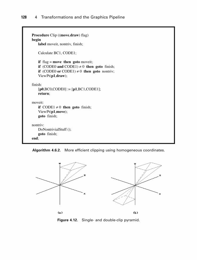
There are some limitations to Blinn’s clipping algorithm. Although they tend tobe more theoretical than practical, one should be aware of them. The problem is thatone is clipping to the infinite inverted pyramid in homogeneous coordinate spaceshown in Figure 4.12(a) when, in fact, one should be clipping to the double pyramidshown in Figure 4.12(b). The points in the negative pyramid will also project to thevisible region. On the other hand, the basic graphics pipeline that we have beendescribing will not introduce any negative w’s and so this problem will not arise here.The problem arises only if negative w-coordinates are introduced explicitly or if onewants to represent infinite segments (the complement of a normal segment in a line).If one does want to handle such cases, the quickest way to do it is to draw the worldtwice, once as described above and then a second time, where the matrix that mapsfrom shape to clip coordinates is multiplied by -1.

4.6 Clipping 127

reahomogeneous point p0, p1;

l BC0,BC16-bit word CODE0,CODE1;

Procedure Clip ((move,draw) flag) {We assume that p0, BC0, and CODE0 have been defined. We clip [p0, p1]}begin

Calculate BC1, CODE1;

case flag ofmove : DoMoveStuff ();draw : DoDrawStuff ();

end;

{ Update globals } [p0,BC0,CODE0] := [p1,BC1,CODE1];

end;

Procedure DoMoveStuff ()if CODE1 = 0 then ViewPt (p1,move);

Procedure DoDrawStuff ()if (CODE0 and CODE1) = 0 then

beginif (CODE0 or CODE1) = 0

then ViewPt (p1,draw)else DoNontrivialStuff ()

end;

Algorithm 4.6.1. Abstract programs for clipping using homogeneous coordinates.

GOS04 5/5/2005 6:18 PM Page 127


Procedure Clip ((move,draw) flag) begin

label moveit, nontriv, finish;

Calculate BC1, CODE1;

if flag = move then goto moveit;if (CODE0 and CODE1) π 0 then goto finish; if (CODE0 or CODE1) π 0 then goto nontriv;ViewPt(p1,draw);

finish:[p0,BC0,CODE0] := [p1,BC1,CODE1];return;

moveit:if CODE1 π 0 then goto finish; ViewPt(p1,move);goto finish;

nontriv:DoNontrivialStuff ();goto finish;

end;

Algorithm 4.6.2. More efficient clipping using homogeneous coordinates.

Figure 4.12. Single- and double-clip pyramid.

GOS04 5/5/2005 6:18 PM Page 128

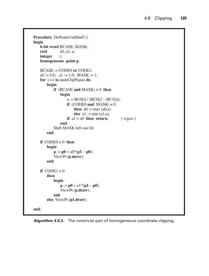
Algorithm 4.6.3. The nontrivial part of homogeneous coordinate clipping.

4.6 Clipping 129

Procedure DoNontrivialStuff ()begin

6-bit word BCASE, MASK; realinteger i;

a0, a1, a;

homogeneous point p;

BCASE := CODE0 or CODE1;a0 := 0.0; a1 := 1.0; MASK := 1;for i:=1 to numClipPlanes do

beginif (BCASE and MASK) π 0 then

begina := BC0[i] / (BC0[i] - BC1[i]);if (CODE0 and MASK) π 0

then a0 := max (a0,a)else a1 := min (a1,a);

if a1 < a0 then return; { reject } end;

Shift MASK left one bit end;

if CODE0 π 0 thenbegin

p := p0 + a0*(p1 - p0);ViewPt (p,move);

end;

if CODE1 π 0 then

beginp := p0 + a1*(p1 - p0);ViewPt (p,draw);

endelse ViewPt (p1,draw);

end;

GOS04 5/5/2005 6:18 PM Page 129

4.7 Putting It All Together

We are finally ready to put all the pieces together. See Figure 4.1 again. Starting withsome shape we are initially in shape coordinates. We then

(1) transform to world coordinates(2) transform from world to homogeneous clip coordinates by composing

TworÆcam and TcamÆhclip(3) clip(4) project (x,y,z,w) down to (x/w,y/w,z/w) in the unit cube of clip space with Tproj(5) map the unit square in the x-y plane of clip space to the viewport(6) map from the viewport to pixel space

With respect to (4), note that using a front clipping plane does have the advantagethat we do not have to worry about a division by zero. Almost, but not quite. Thereis the very special case of (0,0,0,0) that could occur and hence one needs to check forit (Exercise 4.7.1). It would be complicated to eliminate this case.

Also, because of the clipping step, Blinn suggests a more complete version of thewindow-to-pixel map than shown in Figure 4.9. See Figure 4.13. The square [0,1] ¥[0,1] represents the clipping. This allows one to handle the situation shown in Figure4.14, where the viewport goes outside the valid NDC range quite easily. One pulls backthe clipped viewport

to the rectangle

and then uses that rectangle as the window. Only the transformation TcamÆhclip needsto be changed, not the clipping algorithm.

Blinn’s approach is nice, but there may not be any need for this generality. A muchsimpler scheme that works quite well is to forget about the NDC by incorporating thehardware aspect ratio rh into the window size. Let

wx wx wy wymin, max min, max[ ] ¥ [ ]

ux ux uy uymin, max min, max[ ] ¥ [ ]


Figure 4.13. From window to pixelcoordinates.

GOS04 5/5/2005 6:18 PM Page 130

be the current viewport. Then fix the window to be the rectangle [-1,1] ¥ [-b,b], where

Now map directly from [0,1] ¥ [0,1] to pixel space. With this window and the viewtransformations discussed in this chapter, circles will look like circles.

We close with a final remark on clipping. Clipping is expensive and therefore wewould rather not do it! In future chapters we shall discuss ways one can often avoidit (by using bounding boxes, the convex hull property of splines, etc.).

4.8 Stereo Views

Occasionally, it is useful to allow the origin of the view plane to be a point other thanthe one directly in front of the camera. One such case is where one wants to computestereo views. This involves computing two views, one for each eye.

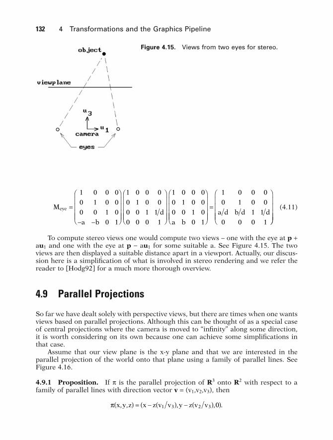
The Eye Coordinate System. Given a camera, let (u1,u2,u3,p) be the camera coor-dinate system, where the vectors u1, u2, and u3 are defined by equation (4.1) If we think of one eye as being located at p + au1 + bu2, then the eye coordinate systemwith respect to the given camera and some a, b Œ R is defined by the frame (u1,u2,u3,p + au1 + bu2). If a = b = 0, then this is the same as the camera coordinatesystem.

It is easy to see that if the coordinates of a point p in camera coordinates is (x,y,z),then the coordinates of that same point in eye coordinates are (x - a,y - b,z). Fur-thermore, if p projects to (x¢,y¢,d) in eye coordinates, then it projects to (x¢ + a,y¢ +b,d) in camera coordinates. It follows that, using homogeneous coordinates, the onlydifference in computing the view in camera coordinates to computing it in eye coor-dinates amounts to replacing the matrix Mpersp in equation (4.9) by

b r y y x xh= -( ) -( )max min max min .

vpx vpx vpy vpymin, max min, max[ ] ¥ [ ]

4.8 Stereo Views 131

Figure 4.14. General window andviewport example.

GOS04 5/5/2005 6:18 PM Page 131

(4.11)

To compute stereo views one would compute two views – one with the eye at p +au1 and one with the eye at p - au1 for some suitable a. See Figure 4.15. The twoviews are then displayed a suitable distance apart in a viewport. Actually, our discus-sion here is a simplification of what is involved in stereo rendering and we refer thereader to [Hodg92] for a much more thorough overview.

4.9 Parallel Projections

So far we have dealt solely with perspective views, but there are times when one wantsviews based on parallel projections. Although this can be thought of as a special caseof central projections where the camera is moved to “infinity” along some direction,it is worth considering on its own because one can achieve some simplifications inthat case.

Assume that our view plane is the x-y plane and that we are interested in the parallel projection of the world onto that plane using a family of parallel lines. SeeFigure 4.16.

4.9.1 Proposition. If p is the parallel projection of R3 onto R2 with respect to afamily of parallel lines with direction vector v = (v1,v2,v3), then

p x y z x z v v y z v v, , , , .( ) = - ( ) - ( )( )1 3 2 3 0

M

a b

d

a b

a d b d deye =

- -

Ê

Ë

ÁÁÁÁ

ˆ

¯

˜˜˜̃

Ê

Ë

ÁÁÁÁ

ˆ

¯

˜˜˜̃

Ê

Ë

ÁÁÁÁ

ˆ

¯

˜˜˜̃

=

Ê

Ë

ÁÁÁÁ

ˆ1 0 0 0

0 1 0 0

0 0 1 0

0 1

1 0 0 0

0 1 0 0

0 0 1 1

0 0 0 1

1 0 0 0

0 1 0 0

0 0 1 0

0 1

1 0 0 0

0 1 0 0

1 1

0 0 0 1 ¯̄

˜˜˜̃


Figure 4.15. Views from two eyes for stereo.

GOS04 5/5/2005 6:18 PM Page 132

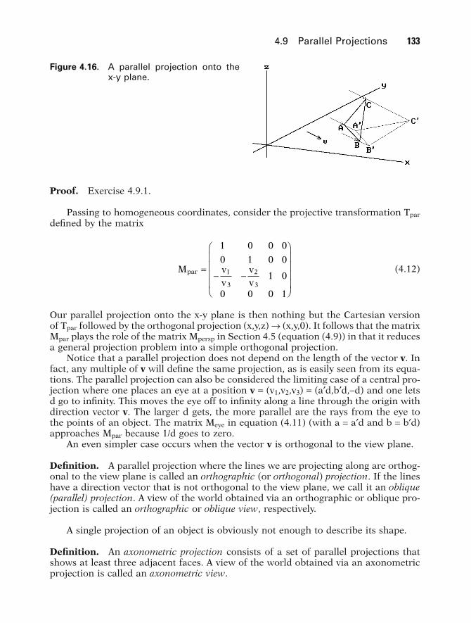
Proof. Exercise 4.9.1.

Passing to homogeneous coordinates, consider the projective transformation Tpardefined by the matrix

(4.12)

Our parallel projection onto the x-y plane is then nothing but the Cartesian versionof Tpar followed by the orthogonal projection (x,y,z) Æ (x,y,0). It follows that the matrixMpar plays the role of the matrix Mpersp in Section 4.5 (equation (4.9)) in that it reducesa general projection problem into a simple orthogonal projection.

Notice that a parallel projection does not depend on the length of the vector v. Infact, any multiple of v will define the same projection, as is easily seen from its equa-tions. The parallel projection can also be considered the limiting case of a central pro-jection where one places an eye at a position v = (v1,v2,v3) = (a¢d,b¢d,-d) and one letsd go to infinity. This moves the eye off to infinity along a line through the origin withdirection vector v. The larger d gets, the more parallel are the rays from the eye tothe points of an object. The matrix Meye in equation (4.11) (with a = a¢d and b = b¢d)approaches Mpar because 1/d goes to zero.

An even simpler case occurs when the vector v is orthogonal to the view plane.

Definition. A parallel projection where the lines we are projecting along are orthog-onal to the view plane is called an orthographic (or orthogonal) projection. If the lineshave a direction vector that is not orthogonal to the view plane, we call it an oblique(parallel) projection. A view of the world obtained via an orthographic or oblique pro-jection is called an orthographic or oblique view, respectively.

A single projection of an object is obviously not enough to describe its shape.

Definition. An axonometric projection consists of a set of parallel projections thatshows at least three adjacent faces. A view of the world obtained via an axonometricprojection is called an axonometric view.

M vv

vv

par =- -

Ê

Ë

ÁÁÁÁ

ˆ

¯

˜˜˜˜

1 0 0 0

0 1 0 0

1 0

0 0 0 1

1

3

2

3

4.9 Parallel Projections 133

Figure 4.16. A parallel projection onto the x-y plane.

GOS04 5/5/2005 6:18 PM Page 133

In engineering drawings one often shows a perspective view along with threeorthographic views – a top, front, and side view, corresponding to looking along thez-, y-, and x-axis, respectively. See Figure 4.17. For a more detailed taxonomy of pro-jections see [RogA90].

Finally, in a three-dimensional graphics program one might want to do some 2dgraphics. For example, one might want to let a user define curves in the plane. Ratherthan maintaining a separate 2d structure for these planar objects it would be moreconvenient to think of them as 3d objects. Using the orthographic projection, one cansimulate a 2d world for the user.

4.10 Homogeneous Coordinates: Pro and Con

The computer graphics pipeline as we have described it made use of homogeneouscoordinates when it came to clipping. The given reason for this was that it avoids adivision by zero problem. How about using homogeneous coordinates and matriceseverywhere? This section looks at some issues related to this question. We shall seethat both mathematical and practical considerations come into play.

Disadvantages of the Homogeneous Coordinate Representation. The main dis-advantage has to do with efficiency. First, it takes more space to store 4-tuples and 4¥ 4 matrices than 3-tuples and 3 ¥ 4 matrices (frames). Second, 4 ¥ 4 matrices needmore multiplications and additions to act on a point than 3 ¥ 4 matrices. Another dis-advantage is that homogenous coordinates are less easy to understand than Cartesiancoordinates.

Advantages of the Homogeneous Coordinate Representation. In a word, theadvantage is uniformity. The composite of transformations can be dealt with in a moreuniform way (we simply do matrix multiplication) and certain shape manipulationsbecome easier using a homogeneous matrix for the shape-to-world coordinate system


Figure 4.17. Perspective and orthographicviews of a 2 ¥ 5 ¥ 3 block.

GOS04 5/5/2005 6:18 PM Page 134

transformation. Furthermore, computer hardware can be optimized to deal with 4 ¥4 matrices to more than compensate for the inefficiency of computation issue men-tioned above.

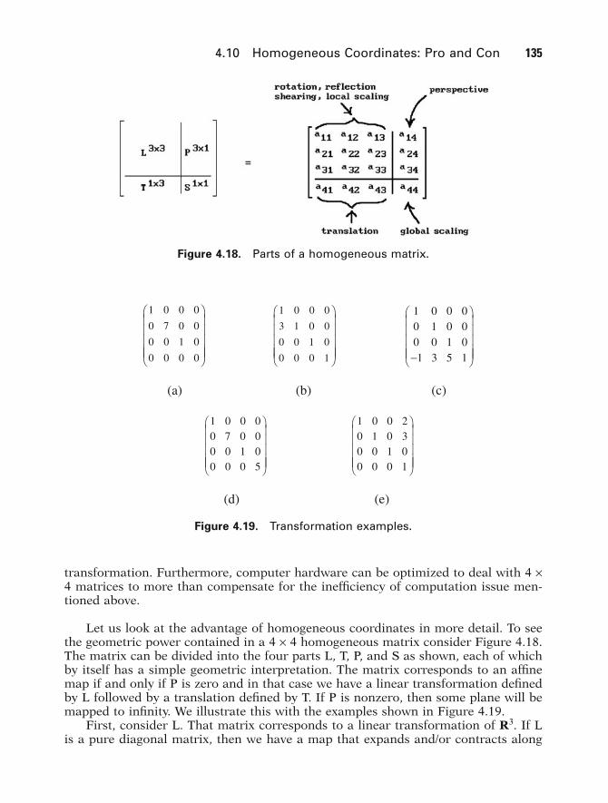
Let us look at the advantage of homogeneous coordinates in more detail. To seethe geometric power contained in a 4 ¥ 4 homogeneous matrix consider Figure 4.18.The matrix can be divided into the four parts L, T, P, and S as shown, each of whichby itself has a simple geometric interpretation. The matrix corresponds to an affinemap if and only if P is zero and in that case we have a linear transformation definedby L followed by a translation defined by T. If P is nonzero, then some plane will bemapped to infinity. We illustrate this with the examples shown in Figure 4.19.

First, consider L. That matrix corresponds to a linear transformation of R3. If Lis a pure diagonal matrix, then we have a map that expands and/or contracts along

4.10 Homogeneous Coordinates: Pro and Con 135

Figure 4.18. Parts of a homogeneous matrix.

1 0 0 0

0 7 0 0

0 0 1 0

0 0 0 0

Ê ˆÁ ˜Á ˜Á ˜Á ˜Á ˜Ë ¯

1 0 0 0

3 1 0 0

0 0 1 0

0 0 0 1

Ê ˆÁ ˜Á ˜Á ˜Á ˜Á ˜Ë ¯

1 0 0 00 1 0 00 0 1 01 3 5 1

Ê ˆÁ ˜Á ˜Á ˜Á ˜Á ˜Ë ¯-

(a) (b) (c)

1 0 0 00 7 0 00 0 1 00 0 0 5

Ê ˆÁ ˜Á ˜Á ˜Á ˜Á ˜Ë ¯

1 0 0 20 1 0 30 0 1 00 0 0 1

Ê ˆÁ ˜Á ˜Á ˜Á ˜Á ˜Ë ¯

(d) (e)

Figure 4.19. Transformation examples.

GOS04 5/5/2005 6:18 PM Page 135

the x, y, or, z axis. For example, the map in Figure 4.19(a) sends the point (x,y,z) tothe point (x,7y,z), which expands everything by a factor of 7 in the y direction.

A lower triangular matrix causes what is called a shear. What this means is thatthe map corresponds to sliding the world along a line while expanding or contract-ing in a possibly not constant manner along a family of lines not parallel to the firstline. The same thing holds for upper triangular matrices. For example, consider thematrix M in Figure 4.19(b). The point (x,y,z) gets sent to (x + 3y,y,z). Points get movedhorizontally. The bigger the y-coordinate is, the more the point is moved. Note thatthis map is really an extension of a map of the plane.

Next, consider the map in Figure 4.19(c). This map sends the point (x,y,z) to (x -1,y + 3,z + 5) and is just a simple translation by the vector (-1,3,5). The map in Figure4.19(d) sends the homogenous point (x,y,z,1) to (x,7y,z,5), in other words, (x,y,z) issent to (x/5,7y/5,z/5), which is just a global scaling. Finally, the map in Figure 4.19(e)sends (x,y,z) to (x/(2x + 3y + 1), y/(2x + 3y + 1), z/(2x + 3y + 1)). The plane 2x + 3y + 1= 0 gets sent to infinity. The map is a two-point perspective map with vanishing pointsfor lines parallel to the x- or y-axes.

We finish this section by describing a way to visualize homogeneous coordinatesand why some caution should be exercised when using them.

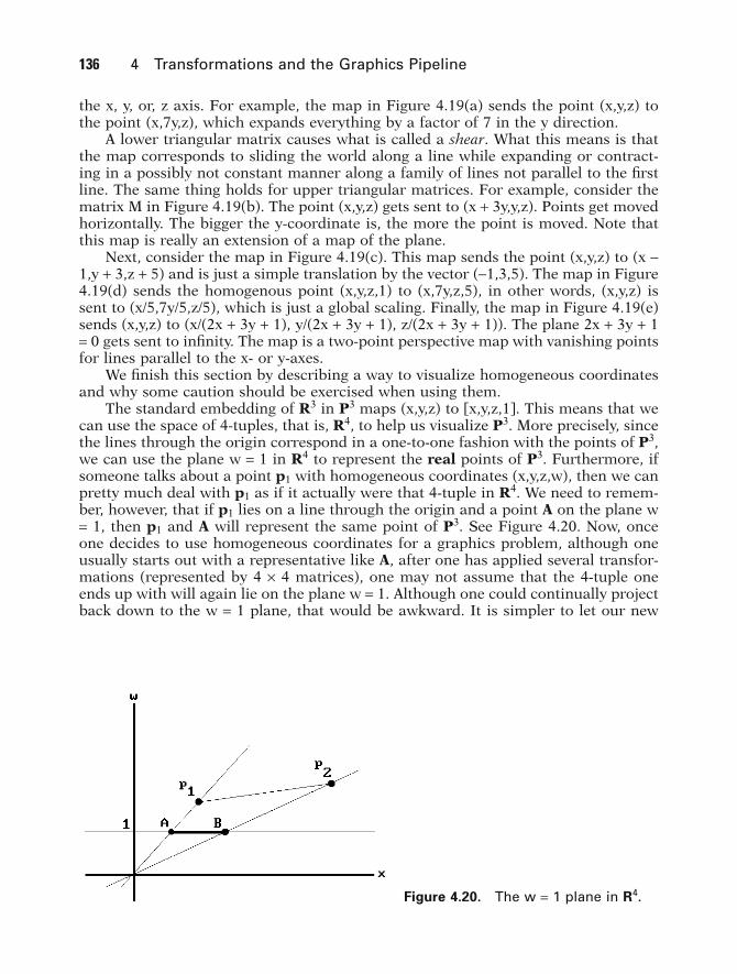
The standard embedding of R3 in P3 maps (x,y,z) to [x,y,z,1]. This means that wecan use the space of 4-tuples, that is, R4, to help us visualize P3. More precisely, sincethe lines through the origin correspond in a one-to-one fashion with the points of P3,we can use the plane w = 1 in R4 to represent the real points of P3. Furthermore, ifsomeone talks about a point p1 with homogeneous coordinates (x,y,z,w), then we canpretty much deal with p1 as if it actually were that 4-tuple in R4. We need to remem-ber, however, that if p1 lies on a line through the origin and a point A on the plane w= 1, then p1 and A will represent the same point of P3. See Figure 4.20. Now, onceone decides to use homogeneous coordinates for a graphics problem, although oneusually starts out with a representative like A, after one has applied several transfor-mations (represented by 4 ¥ 4 matrices), one may not assume that the 4-tuple oneends up with will again lie on the plane w = 1. Although one could continually projectback down to the w = 1 plane, that would be awkward. It is simpler to let our new


Figure 4.20. The w = 1 plane in R4.

GOS04 5/5/2005 6:18 PM Page 136

points float around in R4 and only worry about projecting back to the “real” world atthe end. There will be no problems as long as we deal with individual points. Prob-lems can arise though as soon as we deal with nondiscrete sets.

In affine geometry, segments, for example, are completely determined by their end-points and one can maintain complete information about a segment simply by keepingtrack of its endpoints. More generally, in affine geometry, the boundary of objectsusually determines a well-defined “inside,” and once we know what has happened tothe boundary we know what happened to its “inside.” A circle in the plane divides theplane into two parts, the “inside,” which is the bounded part, and the “outside,” whichis the unbounded part. This is not the case in projective geometry, where it is notalways clear what is “inside” or “outside” of a set. Analogies with the circle and spheremake this point clearer. Two points on a circle divide the circle into two curvilinearsegments. Which is the “inside” of the two points? A circle divides a sphere into twocurvilinear disks. Which is the “interior” of the circle?

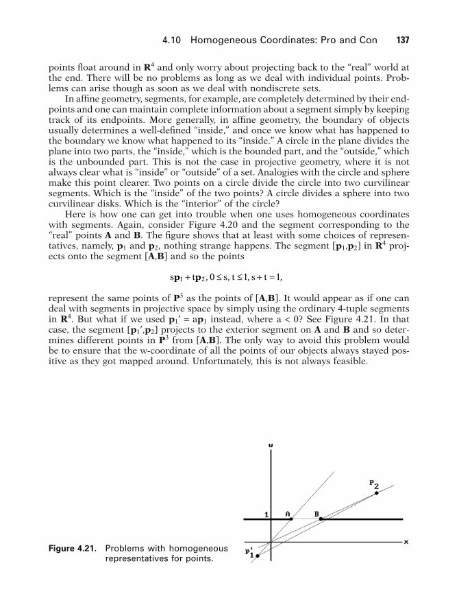
Here is how one can get into trouble when one uses homogeneous coordinateswith segments. Again, consider Figure 4.20 and the segment corresponding to the“real” points A and B. The figure shows that at least with some choices of represen-tatives, namely, p1 and p2, nothing strange happens. The segment [p1,p2] in R4 proj-ects onto the segment [A,B] and so the points

represent the same points of P3 as the points of [A,B]. It would appear as if one candeal with segments in projective space by simply using the ordinary 4-tuple segmentsin R4. But what if we used p1¢ = ap1 instead, where a < 0? See Figure 4.21. In thatcase, the segment [p1¢,p2] projects to the exterior segment on A and B and so deter-mines different points in P3 from [A,B]. The only way to avoid this problem wouldbe to ensure that the w-coordinate of all the points of our objects always stayed pos-itive as they got mapped around. Unfortunately, this is not always feasible.

s t s t s tp p1 2 0 1 1+ £ £ + =, , , ,

4.10 Homogeneous Coordinates: Pro and Con 137

Figure 4.21. Problems with homogeneousrepresentatives for points.

GOS04 5/5/2005 6:18 PM Page 137

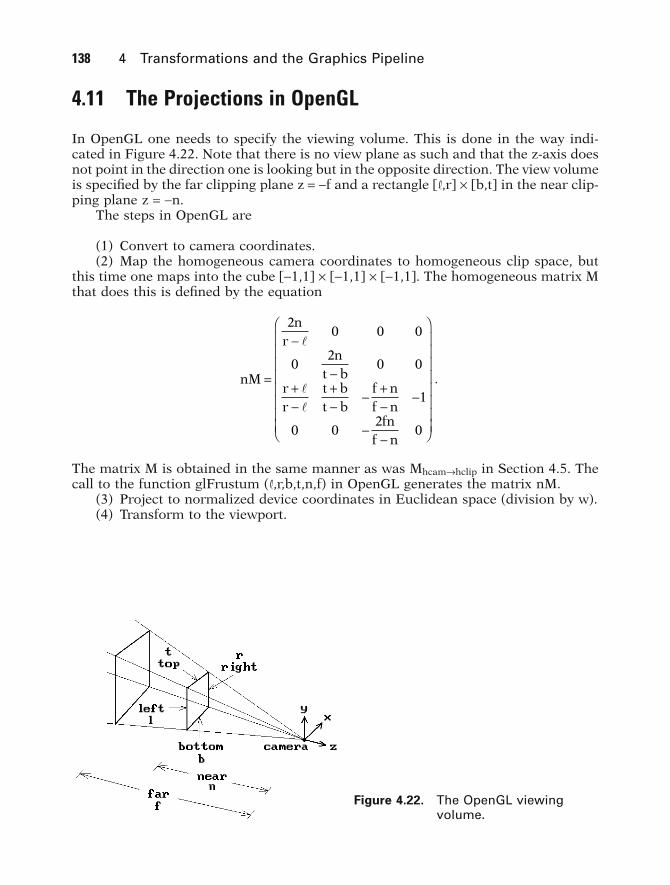
4.11 The Projections in OpenGL

In OpenGL one needs to specify the viewing volume. This is done in the way indi-cated in Figure 4.22. Note that there is no view plane as such and that the z-axis doesnot point in the direction one is looking but in the opposite direction. The view volumeis specified by the far clipping plane z = -f and a rectangle [R,r] ¥ [b,t] in the near clip-ping plane z = -n.

The steps in OpenGL are

(1) Convert to camera coordinates.(2) Map the homogeneous camera coordinates to homogeneous clip space, but

this time one maps into the cube [-1,1] ¥ [-1,1] ¥ [-1,1]. The homogeneous matrix Mthat does this is defined by the equation

The matrix M is obtained in the same manner as was MhcamÆhclip in Section 4.5. Thecall to the function glFrustum (R,r,b,t,n,f) in OpenGL generates the matrix nM.

(3) Project to normalized device coordinates in Euclidean space (division by w).(4) Transform to the viewport.

nM

nr

nt b

rr

t bt b

f nf n

fnf n

=

-

-+-

+-

-+-

-

--

Ê

Ë

ÁÁÁÁÁÁÁÁ

ˆ

¯

˜˜˜˜˜˜˜˜

20 0 0

02

0 0

1

0 02

0

l

l

l


Figure 4.22. The OpenGL viewingvolume.

.

GOS04 5/5/2005 6:18 PM Page 138

4.12 Reconstruction

Ignoring clipping, which we shall in this section, by using homogeneous coordinatesthe mathematics in our discussion of the graphics pipeline basically reduced to anequation of the form

(4.13)

where M was a 4 ¥ 3 matrix, a Œ R4, and b Œ R3. The given quantities were the matrixM, computed from the given camera, and a point in the world that determined a. Wethen used equation (4.13) to compute b and the corresponding point in the view plane.Our goal here is to give a brief look at basic aspects of two types of inverse problems.For additional details see [PenP86]. For a much more thorough and mathematicaldiscussion of this section’s topic see [FauL01].

The Object Reconstruction Problem. Can one determine the point in the worldknowing one or more points in the view plane to which it projected with respect to agiven camera or cameras?

The Camera Calibration Problem. Can one determine the world-to-view-planetransformation if we know some world points and where they get mapped in the viewplane?

Engineers have long used two-dimensional drawings of orthogonal projections ofthree-dimensional objects to describe these objects. The human brain is quite adeptat doing this but the mathematics behind this or the more general problem of recon-structing objects from two-dimensional projections using arbitrary projective trans-formations is not at all easy. Lots of work has been done to come up with efficientsolutions, even in what might seem like the simpler case of orthographic views. See,for example, [ShiS98]. Given three orthographic views of a point (x,y,z), say a front,side, and top view, one would get six constraints on the three values x, y, and z. Suchoverconstrained systems, where the values themselves might not be totally accuratein practice, are typical in reconstruction problems and the best that one can hope foris a best approximation to the answer.

Before describing solutions to our two reconstruction problems, we need toaddress a complication related to homogeneous coordinates. If we consider projec-tive space as equivalence classes [x] of real tuples x, then mathematically we are reallydealing with a map

(4.14)

Equation (4.13) had simply replaced equation (4.14) with an equation of representa-tives a, M, and b for p, T, and q, respectively. The representatives are only unique upto scalar multiple. If we are given p and T and want to determine q, then we are freeto choose any representatives for p and T. The problems in this section, however,involve solving for p given T and b or solving for T given p and q. In these cases, we

T

T

: P P

p q p

3 2ÆÆ = ( )

a bM = ,

4.12 Reconstruction 139

GOS04 5/5/2005 6:18 PM Page 139

cannot assume that the representatives in equation (4.13) all have a certain form. Wemust allow for the scalar multiple in the choice of representatives at least to somedegree. Fortunately, however, the equations can be rewritten in a more convenientform that eliminates any explicit reference to such scalar multiples. It turns out thatwe can always concentrate the scalar multiple in the “b” vector of equation (4.13).Therefore, rather than choosing the usual representative of the form b = (b1,b2,1) for[b], we can allow for scalar multiples by expressing the representative in the form

(4.15)

Let a = (a1,a2,a3,a4) and M = (mij). Let mj = (m1j,m2j,m3j,m4j), j = 1,2,3, be the columnvectors of M. Equation (4.13) now becomes

It follows that c = a•m3. Substituting for c and moving everything to the left, equa-tion (4.13) can be replaced by the equations

(4.16a)

(4.16b)

It is this form of equation (4.13) that will be used in computations below. They havea scalar multiple for b built into them.

After these preliminaries, we proceed to a solution for the first of our two recon-struction problems. The object reconstruction problem is basically a question ofwhether equation (4.13) determines a if M and b are known. Obviously, a single pointb is not enough because that would only determine a ray from the camera and provideno depth information. If we assume that we know the projection of a point withrespect to two cameras, then we shall get two equations

(4.17a)

(4.17b)

At this point we run into the scalar multiple problem for homogeneous coordinatesdiscussed above. In the present case we may assume that M¢ = (mij¢) and M≤ = (mij≤)are two fixed predetermined representatives for our projections and that we arelooking for a normalized tuple a = (a1,a2,a3,1) as long as we allow a scalar multipleambiguity in b¢ = (c¢b1¢,c¢b2¢,c¢) and b≤ = (c≤b1≤,c≤b2≤,c≤). Expressing equations (4.17)in the form (4.16) leads, after some rewriting, to the matrix equation

(4.18)

where

A

m b m m b m m b m m b m

m b m m b m m b m m b m

m b m m b m m

=

¢ - ¢ ¢ ¢ - ¢ ¢ ¢¢ - ¢¢ ¢¢ ¢¢ - ¢¢ ¢¢

¢ - ¢ ¢ ¢ - ¢ ¢ ¢¢ - ¢¢ ¢¢ ¢¢ - ¢¢ ¢¢

¢ - ¢ ¢ ¢ - ¢ ¢

11 1 31 21 2 31 11 1 31 21 1 31

12 1 32 22 2 32 12 1 32 22 1 32

13 1 33 23 2 33 13¢¢¢ - ¢¢ ¢¢ ¢¢ - ¢¢ ¢¢

Ê

Ë

ÁÁÁ

ˆ

¯

˜˜˜b m m b m1 33 23 1 33

a a a A1 2 3( ) = d,

a b¢¢ = ¢¢M .

a b¢ = ¢M

a m m∑ -( ) =2 2 3 0b .

a m m∑ -( ) =1 1 3 0b

a m a m a m∑ ∑ ∑( ) = ◊ ◊( )1 2 3 1 2, , , , .c b c b c

b = ◊ ◊( )c b c b c1 2, , .


GOS04 5/5/2005 6:18 PM Page 140

and

This gives four equations in three unknowns. Such an overdetermined system doesnot have a solution in general; however, if we can ensure that the matrix A has rankthree, then there is a least squares approximation solution

(4.19)

using the generalized matrix inverse A+ (see Theorem 1.11.6 in [AgoM05]).Next, consider the camera calibration problem. Mathematically, the problem is to

compute M if equation (4.13) holds for known points ai and bi, i = 1, 2, . . . , k. Thistime around, we cannot normalize the ai and shall assume that ai = (ai1,ai2,ai3,ai4) andbi = (cibi1,cibi2,ci). It is convenient to rewrite equations (4.16) in the form

(4.20a)

(4.20b)

We leave it as an exercise to show that equations (4.20) can be written in matrix formas

where

and

This overdetermined homogeneous system in twelve unknowns mij will again have aleast squares approximation solution that can be found with the aid of a generalizedinverse provided that n is not zero.

4.13 Robotics and Animation

This section is mainly intended as an example of frames and transformations and howthe former can greatly facilitate the study of the latter, but it also enables us to givea brief introduction to the subject of the kinematics of robot arms. Even though wecan only cover some very simple aspects of robotics here, we cover enough so thatthe reader will learn something about what is involved in animating figures.

n = ( )m m m m m m m m m m m m11 21 31 41 12 22 32 42 13 23 33 43 .

A

b b b b b b

T Tk

T

T Tk

T

T Tn

T T Tn n

T=

- - - - - -

Ê

Ë

ÁÁÁ

ˆ

¯

˜˜˜

a a a 0 0 0

0 0 0 a a a

a a a a a a

1 2

1 2

11 1 21 1 1 1 12 1 22 1 2

L L

L L

L L

n 0A = ,

m a m a2 3 2 0∑ - ∑ =i i ib .

m a m a1 3 1 0∑ - ∑ =i i ib

a a a A A AAT T1 2 3

1( ) = = ( )+ -d d .

d = ¢ ¢ - ¢ ¢ ¢ - ¢ ≤ ≤ - ≤ ≤ ≤ - ≤( )b m m b m m b m m b m m1 34 14 2 34 24 1 34 14 2 34 24 .

4.13 Robotics and Animation 141

GOS04 5/5/2005 6:18 PM Page 141

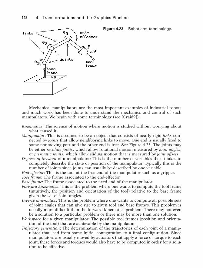
Mechanical manipulators are the most important examples of industrial robotsand much work has been done to understand the mechanics and control of suchmanipulators. We begin with some terminology (see [Crai89]).

Kinematics: The science of motion where motion is studied without worrying aboutwhat caused it.

Manipulator: This is assumed to be an object that consists of nearly rigid links con-nected by joints that allow neighboring links to move. One end is usually fixed tosome nonmoving part and the other end is free. See Figure 4.23. The joints maybe either revolute joints, which allow rotational motion measured by joint angles,or prismatic joints, which allow sliding motion that is measured by joint offsets.

Degrees of freedom of a manipulator: This is the number of variables that it takes tocompletely describe the state or position of the manipulator. Typically this is thenumber of joints since joints can usually be described by one variable.

End-effector: This is the tool at the free end of the manipulator such as a gripper.Tool frame: The frame associated to the end-effector.Base frame: The frame associated to the fixed end of the manipulator.Forward kinematics: This is the problem where one wants to compute the tool frame

(intuitively, the position and orientation of the tool) relative to the base framegiven the set of joint angles.

Inverse kinematics: This is the problem where one wants to compute all possible setsof joint angles that can give rise to given tool and base frames. This problem isusually more difficult than the forward kinematics problem. There may not evenbe a solution to a particular problem or there may be more than one solution.

Workspace for a given manipulator: The possible tool frames (position and orienta-tion of the tool) that are achievable by the manipulator.

Trajectory generation: The determination of the trajectories of each joint of a manip-ulator that lead from some initial configuration to a final configuration. Sincemanipulators are usually moved by actuators that apply a force or torque to eachjoint, these forces and torques would also have to be computed in order for a solu-tion to be effective.


Figure 4.23. Robot arm terminology.

GOS04 5/5/2005 6:18 PM Page 142

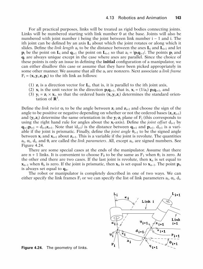
For all practical purposes, links will be treated as rigid bodies connecting joints.Links will be numbered starting with link number 0 at the base. Joints will also benumbered with joint number i being the joint between link number i - 1 and i. Theith joint can be defined by an axis Li about which the joint rotates or along which itslides. Define the link length ai to be the distance between the axes Li and Li+1 and letpi be the point on Li and qi+1 the point on Li+1 so that ai = |piqi+1|. The points pi andqi are always unique except in the case where axes are parallel. Since the choice ofthese points is only an issue in defining the initial configuration of a manipulator, wecan either disallow this case or assume that they have been picked appropriately insome other manner. We assume that all the ai are nonzero. Next associate a link frame Fi = (xi,yi,zi,pi) to the ith link as follows:

(1) zi is a direction vector for Li, that is, it is parallel to the ith joint axis,(2) xi is the unit vector in the direction piqi+1, that is, xi = (1/ai) piqi+1, and(3) yi = zi ¥ xi, so that the ordered basis (xi,yi,zi) determines the standard orien-

tation of R3.

Define the link twist ai to be the angle between zi and zi+1 and choose the sign of theangle to be positive or negative depending on whether or not the ordered bases (zi,zi+1)and (yi,zi) determine the same orientation in the yi-zi plane of Fi (this corresponds tousing the right hand rule for angles about the xi-axis). Define the joint offset di+1 byqi+1pi+1 = di+1zi+1. Note that |di+1| is the distance between qi+1 and pi+1. di+1 is a vari-able if the joint is prismatic. Finally, define the joint angle qi+1 to be the signed anglebetween xi and xi+1 about zi+1. This is a variable if the joint is revolute. The quantitiesai, ai, di, and qi are called the link parameters. All, except ai, are signed numbers. SeeFigure 4.24.

There are some special cases at the ends of the manipulator. Assume that thereare n + 1 links. It is convenient to choose F0 to be the same as F1 when q1 is zero. Atthe other end there are two cases. If the last joint is revolute, then xn is set equal toxn-1 when qn is zero. If the joint is prismatic, then xn is set equal to xn-1. The point pnis always set equal to qn.

The robot or manipulator is completely described in one of two ways. We caneither specify the link frames Fi or we can specify the list of link parameters ai, ai, di,


Figure 4.24. The geometry of links.

GOS04 5/5/2005 6:18 PM Page 143

and qi. Our discussion above basically showed how the latter are derived from theformer. One can also show that the link parameters completely define the frames. Inpractice it is easier for a user to manipulate the link parameters and so the usualproblem is to find the frames given their values. As another example, consider a two-dimensional robot with three links and revolute joints. We can think of this as a specialcase of the general one where all the z-axes of the frames point in the same directionand all the ai and di are zero. Figure 4.25(a) shows the link parameters and Figure4.25(b), the associated frames.

As one can see, frames play a role in defining the state of a robot, but how arethey used to solve problems? Well, the forward kinematic problem is to find the toolframe (“where the tool is”) given the link parameters. This problem will be solved ifwe can determine the transformation Tn, which, given the coordinates of a point p inFn coordinates, finds the coordinates of p with respect to F0. Let dTi, 0 < i £ n, denotethe transformation that maps coordinates relative to Fi to coordinates relative to Fi-1. It follows that

(4.21)

The dTi are relatively easy to compute from the link parameters because they are thecomposition of four simple maps.

The Computation of dTi and Its Homogeneous Matrix dMi. Let Ti(zi, di) denotethe translation with translation vector dizi. Its homogeneous matrix is

1 0 0 0

0 1 0 0

0 0 1 0

0 0 1di

Ê

Ë

ÁÁÁÁ

ˆ

¯

˜˜˜̃

T dT dT dTn n= 1 2o o Lo .


Figure 4.25. Two-dimensional robot arm geometry.

GOS04 5/5/2005 6:18 PM Page 144

Let Ri(zi,qi) denote the rotation about the zi axis of the frame Fi through an angle qi.Its homogeneous matrix is

Let Ti-1(xi-1,ai-1) denote the translation with translation vector ai-1xi-1. Its homoge-neous matrix is

Finally, let Ri-1(xi-1,ai-1) denote the rotation about the xi-1 axis of the frame Fi-1through an angle ai-1. Its homogeneous matrix is

Then

(4.22)

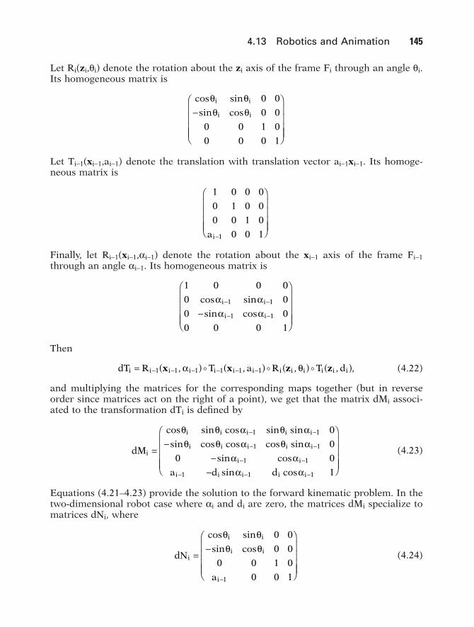
and multiplying the matrices for the corresponding maps together (but in reverseorder since matrices act on the right of a point), we get that the matrix dMi associ-ated to the transformation dTi is defined by

(4.23)

Equations (4.21–4.23) provide the solution to the forward kinematic problem. In thetwo-dimensional robot case where ai and di are zero, the matrices dMi specialize tomatrices dNi, where

(4.24)dN

a

i

i i

i i

i

=-

Ê

Ë

ÁÁÁÁ

ˆ

¯

˜˜˜̃

-

cos sin

sin cos

q qq q

0 0

0 0

0 0 1 0

0 0 11

dM

a d d

i

i i i i i

i i i i i

i i

i i i i i

=-

--

Ê

Ë

ÁÁÁÁ

ˆ

¯

˜˜˜̃

- -

- -

- -

- - -

cos sin cos sin sin

sin cos cos cos sin

sin cos

sin cos

q q a q aq q a q a

a aa a

1 1

1 1

1 1

1 1 1

0

0

0 0

1

dT R T a R T di i i i i i i i i i i i i= ( ) ( ) ( ) ( )- - - - - -1 1 1 1 1 1x x z z, , , , ,a qo o o

1 0 0 0

0 0

0 0

0 0 0 1

1 1

1 1

cos sin

sin cos

a aa a

i i

i i

- -

- --

Ê

Ë

ÁÁÁÁ

ˆ

¯

˜˜˜̃

1 0 0 0

0 1 0 0

0 0 1 0

0 0 11ai-

Ê

Ë

ÁÁÁÁ

ˆ

¯

˜˜˜̃

cos sin

sin cos

q qq qi i

i i

0 0

0 0

0 0 1 0

0 0 0 1

-Ê

Ë

ÁÁÁÁ

ˆ

¯

˜˜˜̃


GOS04 5/5/2005 6:18 PM Page 145

This concludes what we have to say about robotics. For a more in-depth study ofthe subject see [Crai89], [Feat87], or [Paul82]. The description of mechanical manip-ulators in terms of the four link parameters described in this section is usually calledthe Denavit-Hartenberg notation (see [DenH55]).

As is often the case when one is learning something new, a real understanding ofthe issues does not come until one has worked out some concrete examples. The ani-mation programming projects 4.13.1 and 4.13.2 should help in that regard. Here area few comments about how one animates objects. Recall the discussion in Section2.11 for the 2d case. To show motion one again discretizes time and shows a sequenceof still pictures of the world as it would look at increasing times t1, t2, . . . , tn. Onechanges the apparent speed of the motion by changing the size of the time intervalsbetween ti and ti+1, the larger the intervals, the larger the apparent speed. Therefore,to move an object X, one begins by showing the world with the object at its initialposition and then loops through reshowing the world, each time placing the object inits next position.

4.14 Quaternions and In-betweening

This short section describes another aspect of how transformations get used in ani-mation. In particular, we discuss a nice application of quaternions. Unit quaternionsare a more efficient way to represent a rotation of R3 than the standard matrix rep-resentation of SO(3). Chapter 20 provides the mathematical foundation for quater-nions. Other references for the topic of this section are [WatW92], [Hogg92], and[Shoe93].

We recall some basic facts about the correspondence between rotations about theorigin in R3 and unit quaternions. First of all, the quaternion algebra H is just R4

endowed with the quaternion product. The metric on H is the same as that on R4.The standard basis vectors e1, e2, e3, e4 are now denoted by 1, i, j, k, respectively. Thesubspace generated by i, j, and k is identified with R3 by mapping the quaternionai+bj+ck to (a,b,c) and vice versa. The rotation R of R3 through angle q about thedirected line through the origin with unit direction vector n is mapped to the quater-nion q defined by

(4.25)

Conversely, let q = r + ai + bj + ck be a unit quaternion (q Œ S3) and express q in theform

(4.26)

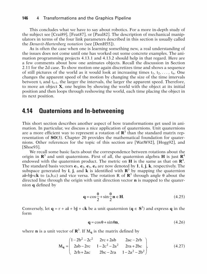
where n is a unit vector of R3. If Mq is the matrix defined by

(4.27)M

b c rc ab ac rb

ab rc c a ra bc

rb ac bc ra a bq =

- - + -- - - ++ - - -

Ê

Ë

ÁÁ

ˆ

¯

˜˜

1 2 2 2 2 2 2

2 2 1 2 2 2 2

2 2 2 2 1 2 2

2 2

2 2

2 2

,

q n= +cos sin ,q q

q n H= + Œcos sin .q q2 2


GOS04 5/5/2005 6:18 PM Page 146

then Mq Œ SO(3) and the map of R3 that sends p to pMq is a rotation Rq about theline through the origin with direction vector n through the angle 2q. This mapping

has the property that Rq = R-q.Now, suppose an object is moved by a one-parameter family of matrices M(s) Œ

SO(3). Assume that we have only specified this family at a fixed set of values si. Howcan we interpolate between these values? In animation such an interpolation is calledin-betweening. A simple interpolation of the form

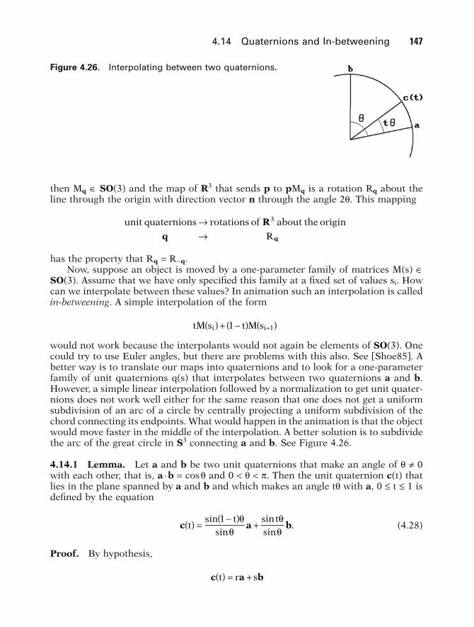
would not work because the interpolants would not again be elements of SO(3). Onecould try to use Euler angles, but there are problems with this also. See [Shoe85]. Abetter way is to translate our maps into quaternions and to look for a one-parameterfamily of unit quaternions q(s) that interpolates between two quaternions a and b.However, a simple linear interpolation followed by a normalization to get unit quater-nions does not work well either for the same reason that one does not get a uniformsubdivision of an arc of a circle by centrally projecting a uniform subdivision of thechord connecting its endpoints. What would happen in the animation is that the objectwould move faster in the middle of the interpolation. A better solution is to subdividethe arc of the great circle in S3 connecting a and b. See Figure 4.26.

4.14.1 Lemma. Let a and b be two unit quaternions that make an angle of q π 0with each other, that is, a ·b = cosq and 0 < q < p. Then the unit quaternion c(t) thatlies in the plane spanned by a and b and which makes an angle tq with a, 0 £ t £ 1 isdefined by the equation

(4.28)

Proof. By hypothesis,

c a bt r s( ) = +

c a btt t( ) =

-( )+

sinsin

sinsin

.1 q

qqq

tM s t M si i( ) + -( ) ( )+1 1

unit quaternions rotations of about the origin

R

ÆÆ

R

q q

3

4.14 Quaternions and In-betweening 147

Figure 4.26. Interpolating between two quaternions.

GOS04 5/5/2005 6:18 PM Page 147

for some real numbers r and s. Taking the dot product of both sides of this equationwith a and b leads to equations

(4.29)

and

(4.30)

Solving equations (4.29) and (4.30) for r and s and using some standard trigonomet-ric identities leads to the stated result.

4.14.2 Example. Let L0 and L1 be the positively directed x- and y-axis, respectively.Let R0 and R1 be the rotations about the directed lines L0 and L1, respectively, throughangle p/3 and let M0 and M1 be the matrices that represent them. If Mt, t Œ [0,1], isthe 1-parameter family of in-betweening matrices in SO(3) between M0 and M1, thenwhat is M1/2?

Solution. The unit direction vectors for L0 and L1 are n0 = (1,0,0) and n1 = (0,1,0),respectively. Therefore, by equation (4.25)

and

are the unit quaternions corresponding to rotation R0 and R1. The angle q betweenq0 and q1 is defined by

It follows that

Using equation (4.28), let

Finally, equation (4.27) implies that

q q q1 2 0 12

142

314

1

14

1

140 2

314

1

7

1

2

1

20= +( ) = + Ê

Ëˆ¯ = + Ê

Ëˆ¯, , , , .

sin cos sincos

.q qq q

= - = =-

=17

4 21

21

2 22 and

cos .q = ∑ =q q0 134

q n1 16 63

212

1 0 0= + = + ( )cos sin , ,p p

q n0 06 63

212

1 0 0= + = + ( )cos sin , ,p p

cos .1-( ) = ( ) ∑ = ∑ +t t r sq c b a b

cost t r sq = ( ) ∑ = + ∑c a b a


GOS04 5/5/2005 6:18 PM Page 148

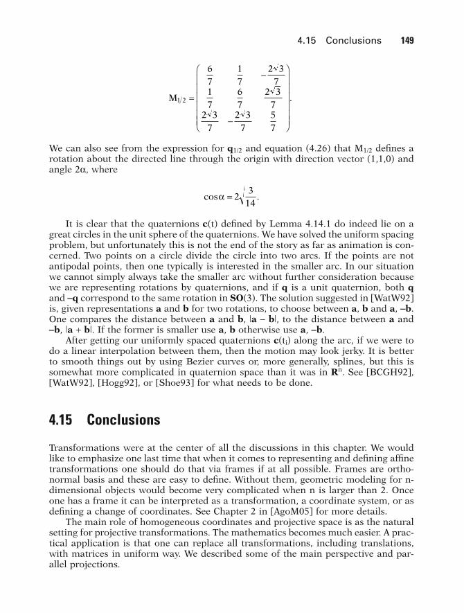
We can also see from the expression for q1/2 and equation (4.26) that M1/2 defines arotation about the directed line through the origin with direction vector (1,1,0) andangle 2a, where

It is clear that the quaternions c(t) defined by Lemma 4.14.1 do indeed lie on agreat circles in the unit sphere of the quaternions. We have solved the uniform spacingproblem, but unfortunately this is not the end of the story as far as animation is con-cerned. Two points on a circle divide the circle into two arcs. If the points are notantipodal points, then one typically is interested in the smaller arc. In our situationwe cannot simply always take the smaller arc without further consideration becausewe are representing rotations by quaternions, and if q is a unit quaternion, both qand -q correspond to the same rotation in SO(3). The solution suggested in [WatW92]is, given representations a and b for two rotations, to choose between a, b and a, -b.One compares the distance between a and b, |a - b|, to the distance between a and-b, |a + b|. If the former is smaller use a, b otherwise use a, -b.

After getting our uniformly spaced quaternions c(ti) along the arc, if we were todo a linear interpolation between them, then the motion may look jerky. It is betterto smooth things out by using Bezier curves or, more generally, splines, but this issomewhat more complicated in quaternion space than it was in Rn. See [BCGH92],[WatW92], [Hogg92], or [Shoe93] for what needs to be done.

4.15 Conclusions

Transformations were at the center of all the discussions in this chapter. We wouldlike to emphasize one last time that when it comes to representing and defining affinetransformations one should do that via frames if at all possible. Frames are ortho-normal basis and these are easy to define. Without them, geometric modeling for n-dimensional objects would become very complicated when n is larger than 2. Onceone has a frame it can be interpreted as a transformation, a coordinate system, or asdefining a change of coordinates. See Chapter 2 in [AgoM05] for more details.

The main role of homogeneous coordinates and projective space is as the naturalsetting for projective transformations. The mathematics becomes much easier. A prac-tical application is that one can replace all transformations, including translations,with matrices in uniform way. We described some of the main perspective and par-allel projections.

cos .a = 23

14

M1 2

67

17

2 37

17

67

2 37

2 37

2 37

57

=

-

-

Ê

Ë

ÁÁÁÁÁÁ

ˆ

¯

˜˜˜˜˜˜

.

4.15 Conclusions 149

GOS04 5/5/2005 6:18 PM Page 149

The discussion in this chapter emphasized a mathematical view of transforma-tions. Let us add a few comments about efficiency because there are times when effi-ciency is more important than clarity. Transformations get used a lot in geometricmodeling and generating them in a systematic way, which usually involves repre-senting them as a composite of primitive ones, involves more arithmetic operationsthan necessary. The papers [Gold90] and [Mill99] describe a more efficient approach.For example, suppose we express an arbitrary affine transformation T of R3 in theform

where M is a 3 ¥ 3 matrix and v is a fixed translation vector. If T is a rotation throughan angle q about a line L through a point q with direction vector w, then it is shownthat

(4.31a)

(4.31b)

where I is the 3 ¥ 3 identity matrix,

and

With this representation, an optimized computation takes 15 multiplications and 10additions to compute M and 9 multiplications and 9 additions to compute v. Thenumber of operations to compute the matrix M and vector v with the “composite-of-transformations” approach would be much greater. See [Gold90] for efficient formu-las for other transformations.

Finally, one topic not discussed much in this book (other than in the documen-tation for the GM and SPACE program) is the user interface of a modeling program,even though this takes up a large percentage of the time needed to develop such aprogram in general. Certain aspects of such a discussion, if we had the space or time,would probably be most appropriate in the context of the topic of this chapter. Thereare lots of interesting issues here as to how one can make it easier for the user todefine the desired view of the world. How to best look at the world is often a majorconcern to a user. How does a user specify a view? How does one control panningand zooming? How does one specify a user’s or the camera’s arbitrary movementthrough the world? In a three-dimensional world this is not always easy if all one hasis a keyboard and a mouse.

A

w w

w w

w ww =

--

-

Ê

ËÁÁ

ˆ

¯˜˜

0

0

0

3 2

3 1

2 1

.

a bƒ =Ê

ËÁÁ

ˆ

¯˜˜

=Ê

ËÁÁ

ˆ

¯˜˜

( )a b a b a b

a b a b a b

a b a b a b

a

a

a

b b b1 1 1 2 1 3

2 1 2 2 2 3

3 1 3 2 3 3

1

2

3

1 2 3 ,

v q Mq= - T,

M I A andw= + -( ) ƒ +cos cos sinq q q1 w w

T M Tp p v( ) = + ,


GOS04 5/5/2005 6:18 PM Page 150

4.16 EXERCISES

Section 4.2

4.2.1 Prove equation (4.3).

4.2.2 Find the world-to-camera coordinates transformation T in two dimensions given the following data: the camera is at (1,4) looking in direction (-1,-3) with the view “plane”(a line) a distance in front of the camera.

4.2.3 Find the world-to-camera coordinates transformation T in three dimensions given thatthe camera is at (2,3,5) looking in direction (-1,2,1) with the view plane a distance 7 infront of the camera.

Section 4.3

4.3.1 A camera is situated at the origin looking in direction v. Find the vanishing points ofthe view defined by lines parallel to the standard unit cube when

(a) v = (2,0,3)(b) v = (0,3,0)(c) v = (3,1,2)

Section 4.5

4.5.1 With regard to Figure 4.11 show that the regions below are mapped as indicated:

Note that z/w denotes the “real” z coordinate of a projective point (x,y,z,w).

4.5.2 Assume that the near and far planes for a camera are z = 2 and z = 51, respectively, incamera coordinates. If the view plane is z = 5, find the matrix MhcamÆhclip.

Section 4.7

4.7.1 Explain how the case (0,0,0,0) can occur.

Section 4.9

4.9.1 Prove Proposition 4.9.1.

4.9.2 Compute the parallel projection of R3 onto the x-y plane in the direction v = (2,1,5).

4.9.3 Compute the parallel projection of R3 onto the plane x - 2y + 3z = 1 in the direction v = (2,1,-3).

-• < < - Æ < < +•- < < Æ -• < <

< < +• Æ < < +

z w z w

z w z w

z w z w

1 1

1 0 0

0 0 1

10

4.16 Exercises 151

GOS04 5/5/2005 6:18 PM Page 151

Section 4.14

4.14.1 Let L0 and L1 be the directed lines through the origin in R3 with direction vectors (1,-1,0) and (1,1,0), respectively. Let R0 and R1 be the rotations about the directed linesL0 and L1, respectively, through angle p/3 and let M0 and M1 be the matrices that rep-resent them. If Mt, t Œ [0,1], is the 1-parameter family of in-betweening matrices inSO(3) between M0 and M1, find M1/2?

Section 4.15

4.15.1 Show that equations (4.31) compute the rotation T correctly.

4.17 PROGRAMMING PROJECTS

Section 4.5

4.5.1 A simpler graphics pipeline

The approach to clipping we described in Section 4.5 is more general than may be needed insome simple situations. This project describes a quick way to deal with clipping if one alreadyhas a two-dimensional clipper implemented. The basic idea is to do the z-clip in three dimen-sions but then to project to the view plane and do the rest of the clipping with the old 2-dimen-sional clipper. Since the far clipping plane is usually not very important, we shall ignore it andonly worry about the near clipping plane. Then a simple graphics pipeline for an object that iseither a point or a segment would go as follows:

(1) Transform any vertex (x,y,z) of the object in shape coordinates to camera coordi-nates (x¢,y¢,z¢).

(2) Clip the resulting point or segment against the near clip plane.

(3) Project any vertex (x¢,y¢,z¢) of the remaining object to the point (x≤,y≤) in the viewplane using the equations

where d is the distance that the view plane is in front of the camera.

Clipping against the near clip plane is essential for two reasons. One is that we do not wantpoints from behind the camera to project to the front. The second is that we want to preventany division by zero. The clipping itself is very easy here. Assume that the near clipping planeis defined in the camera coordinate system by the equation z = dn. Mathematically, clipping asingle point simply amounts to checking if z¢ < dn or not. In the case of a segment, we have tofind the intersection of that segment with the plane.

Consider a world of rectangular blocks for this program. Each block is defined by threereal parameters a, b, and c and a frame f. The basic block is situated at the origin with facesparallel to the coordinate planes and vertices (0,0,0), (a,0,0), (a,0,c), (0,0,c), (0,b,0), (a,b,0),(a,b,c), and (0,b,c) and all other blocks are copies of this block moved by the frame f.

¢¢ =¢¢

¢¢ =¢¢

x dxz

and y dyz

,


GOS04 5/5/2005 6:18 PM Page 152

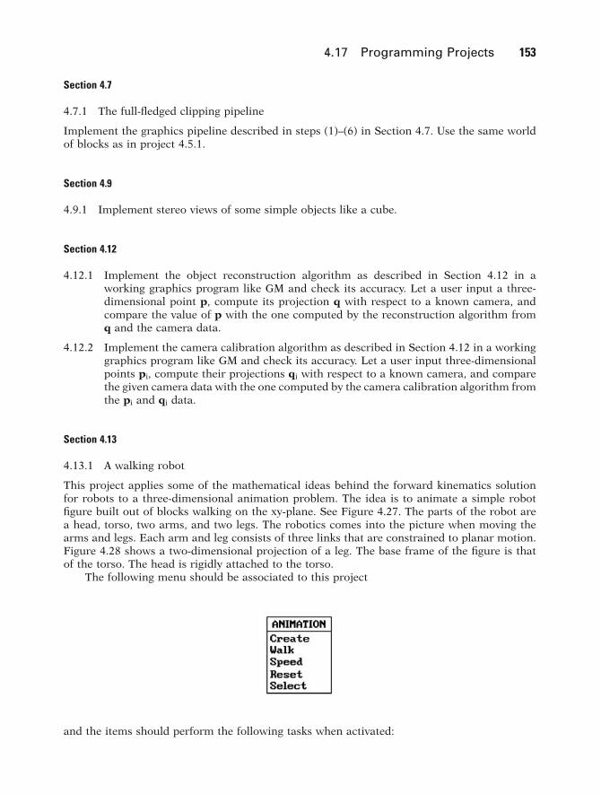
Section 4.7

4.7.1 The full-fledged clipping pipeline

Implement the graphics pipeline described in steps (1)–(6) in Section 4.7. Use the same worldof blocks as in project 4.5.1.

Section 4.9

4.9.1 Implement stereo views of some simple objects like a cube.

Section 4.12

4.12.1 Implement the object reconstruction algorithm as described in Section 4.12 in aworking graphics program like GM and check its accuracy. Let a user input a three-dimensional point p, compute its projection q with respect to a known camera, andcompare the value of p with the one computed by the reconstruction algorithm fromq and the camera data.

4.12.2 Implement the camera calibration algorithm as described in Section 4.12 in a workinggraphics program like GM and check its accuracy. Let a user input three-dimensionalpoints pi, compute their projections qi with respect to a known camera, and comparethe given camera data with the one computed by the camera calibration algorithm fromthe pi and qi data.

Section 4.13

4.13.1 A walking robot

This project applies some of the mathematical ideas behind the forward kinematics solutionfor robots to a three-dimensional animation problem. The idea is to animate a simple robotfigure built out of blocks walking on the xy-plane. See Figure 4.27. The parts of the robot area head, torso, two arms, and two legs. The robotics comes into the picture when moving thearms and legs. Each arm and leg consists of three links that are constrained to planar motion.Figure 4.28 shows a two-dimensional projection of a leg. The base frame of the figure is thatof the torso. The head is rigidly attached to the torso.

The following menu should be associated to this project

4.17 Programming Projects 153

and the items should perform the following tasks when activated:

GOS04 5/5/2005 6:18 PM Page 153

Create: Ask the user for a size and then create a new robot of that given size. At any giventime there is a currently active robot (the one to which the “Walk,” “Speed,” and“Reset” commands apply).

Walk: Ask the user for a number of steps, then walk the robot that many steps in the direc-tion it is facing with its joints moving in a way so that the walk is reasonably closeto a human’s walk.

Speed: Ask the user for a new speed that is a function of the distance between positions atwhich the robot is displayed.

Reset: Resets the robot to its initial configuration.Select: Let the user specify another robot to be the currently active one.

4.13.2 Robot walking along path

Extend project 4.13.1 by associating a path to each robot along which it walks. For example,the robot in Figure 4.27(b) is walking along path C. The default path for a robot (if the userdid not explicitly define one) is a straight line in the direction the robot is pointing.

The menu should now look like


(a) (b)

Figure 4.27. Robots in motion.

Figure 4.28. Two-dimensional link parameters.

GOS04 5/5/2005 6:18 PM Page 154

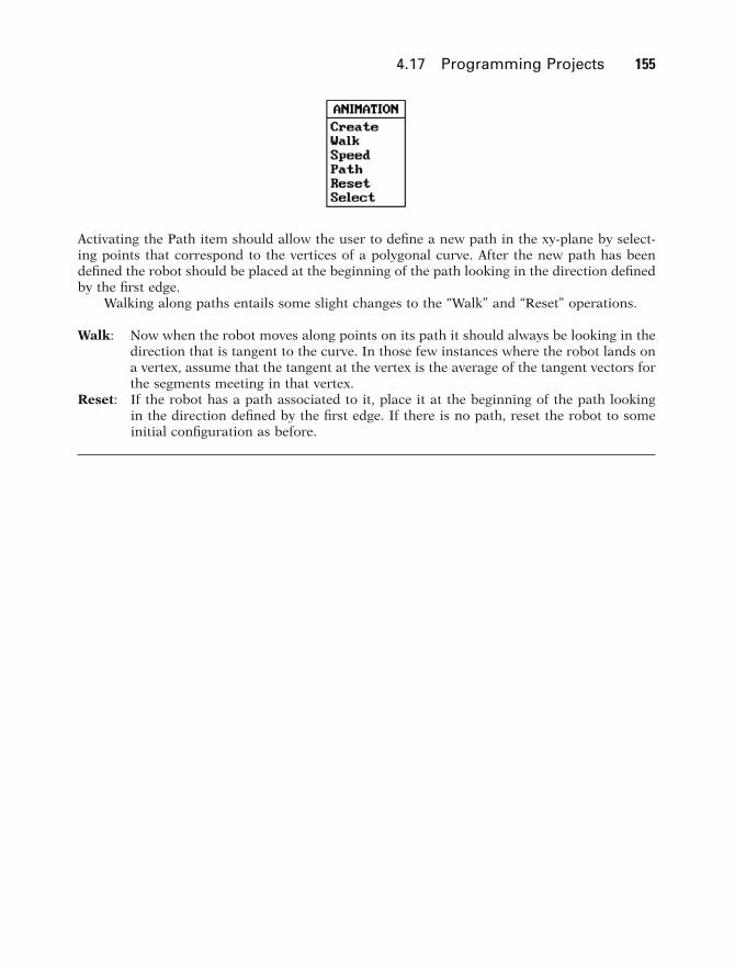
4.17 Programming Projects 155

Activating the Path item should allow the user to define a new path in the xy-plane by select-ing points that correspond to the vertices of a polygonal curve. After the new path has beendefined the robot should be placed at the beginning of the path looking in the direction definedby the first edge.

Walking along paths entails some slight changes to the “Walk” and “Reset” operations.

Walk: Now when the robot moves along points on its path it should always be looking in thedirection that is tangent to the curve. In those few instances where the robot lands ona vertex, assume that the tangent at the vertex is the average of the tangent vectors forthe segments meeting in that vertex.

Reset: If the robot has a path associated to it, place it at the beginning of the path looking in the direction defined by the first edge. If there is no path, reset the robot to someinitial configuration as before.

GOS04 5/5/2005 6:18 PM Page 155

Transformations and the Graphics Pipeline - 南京航空航...

Documents

Transcript of Transformations and the Graphics Pipeline - 南京航空航...