The value of a floor: valuing floorlevel in high-rise condominiums

in San DiegoStephen Conroy, Andrew Narwold and Jonathan Sandy

School of Business Administration, University of San Diego, San Diego,California, USA

Abstract

Purpose – This paper aims to analyze the effect of floor level on condominium prices in San Diego,California. The authors determine whether “higher-floor premiums” exist in the condominium marketfor a large California city. Further, they investigate how the floor premium varies throughout abuilding, particularly whether it is quadratic and whether there is a “penthouse premium” for top-floorunits.

Design/methodology/approach – The paper utilizes a data set of 2,395 condominium salesoccurring in San Diego between 2006 and the second quarter of 2011. Using hedonic pricing analysis,the authors model the housing price as a function of condominium, building and neighborhoodcharacteristics.

Findings – The results suggest that there is a higher-floor premium for condominiums in San Diego.Specifically, an increase in the floor level is associated with about a 2.2 percent increase in sale price.The higher-floor premium appears to be quadratic in price, suggesting that price increases at adecreasing rate above the mean floor level. The authors also find evidence for a penthouse premium,though this effect disappears once “floor” is controlled for in the model.

Originality/value – There has been little direct research on the floor effect in condominium prices.The studies that have used floor level as an explanatory variable have been predominately inSoutheast Asia. The results suggest that the floor effect is more complex than previously modeled.

Keywords Hedonic pricing, Penthouse, Higher-floor premium, Value of floor, Condominium, San Diego,United States of America, Housing, Prices

Paper type Research paper

IntroductionThere is a growing body of research that suggests that higher condominium floorsconfer higher sale prices, controlling for square footage and other relevant attributes.Evidence for this “higher-floor premium,” however, has been somewhat narrowlypresented in two regards. First, reporting of a higher-floor premium has been largelyincidental, as “floor,” “level” or “story” are included merely as control variables forinvestigations of other matters. As such, there is a dearth of analysis of this particularfinding, i.e. whether it is linear, nonlinear, monotonically increasing by floor, etc. Second,the investigations have occurred primarily in Southeast Asia, Hong Kong in particular.

BackgroundMok et al. (1995), estimate a hedonic pricing model for 1,027 condominiums sold inHong Kong in August 1990. While they seem to have little information on thestructural characteristics of the condominium (other than gross floor area and the ageof the building), they do include the floor level of condominium within the building and

The current issue and full text archive of this journal is available at

www.emeraldinsight.com/1753-8270.htm

International Journal of HousingMarkets and Analysis

Vol. 6 No. 2, 2013pp. 197-208

q Emerald Group Publishing Limited1753-8270

DOI 10.1108/IJHMA-01-2012-0003

The valueof a floor

197

whether there is a sea view. Using sales price as the dependent variable, the authorsestimate four different specifications and find floor level to have a positive andsignificant impact on price in all four specifications. Other studies of Hong Kongoffering similar conclusions include So et al. (1997), Chau and Ng (1998), Chau et al.(2001), Tse (2002) and Chau et al. (2003).

Two other studies find similar results for Singapore. Ong (2000) investigates 15 large(over 200 units) residential condominium developments in Singapore from 1988 to 1998and finds that the higher the floor of the unit, the higher the probability of observing asubsequent sale within the time frame studied (i.e. higher turnover rate) and the higherthe (mortgage) prepayment rate. Ong (p. 595) comments that the finding of a higherprobability of a subsequent sale is “consistent with the commonly held perception thatunits on higher floors are more desirable.” Similarly, Sun et al. (2005) analyzecondominium sales data for Singapore from 1990 to 1999 using several models thatcontrol for spatial autocorrelation and find a consistent, positive relationship betweenfloor level and sales price. Chin et al. (2004) examine 442 condominium sales in Malaysiafor the years 1996 and 1998. Through several different specifications, the coefficient onfloor level remains positive and statistically significant.

While there appears to be empirical evidence for a higher-floor effect, why might thisbe the case? We posit two potentially competing theories that could affect higher-floorprices. On one hand, higher floors take longer to reach from the ground floor thusincreasing travel times. Ceteris paribus, this would likely exert a negative influence onprice as higher travel times increase travel costs. The implicit value of time is at the coreof economic theory. Research conducted in a myriad of situations has confirmed thatindividuals place a value on their time and that this can vary based on a variety offactors, including income (i.e. opportunity cost) and impatience. Thus, it should be nosurprise to learn that hedonic pricing models for residential housing often find that,controlling for square footage, distance from the central business district (CBD) isnegatively related to housing prices – driven by the well-known, “negative rentgradient” (Muth, 1969; Mills, 1972; Colwell and Sirmans, 1978; Kau and Sirmans, 1979;Ohkawara, 1985; Coulson and Engle, 1987; So et al., 1997; Chau and Ng, 1998). In short,ceteris paribus, workers prefer to live closer to work in order to reduce travel times.Thus, to the extent that living on higher-floored units in a multi-floored condominiumincreases travel times for residents we might expect the price of condominium units(controlling for other factors) to decline with floor level. At a minimum, this effect – callit the “negative travel effect” – would put negative pressure on prices of higher-flooredcondominium units. This effect is unlikely to occur in the San Diego condominiummarket, which is characterized by fairly new buildings of moderate height.

At the same time, there is considerable evidence that buyers prefer housing that islocated away from traffic or road noise. Brandt and Maennig (2011), for example, findthat doubling road noise in Hamburg, Germany would reduce condominium prices by2.3 percent. Buyers have also been found to value locations and near amenities such asforests (Tyravinen and Miettinen, 2000), lakes (Kilpatrick et al., 2007), trails and greenbelts(Asabere and Huffman, 2009), ponds (Plattner and Campbell, 1978), green spaces(Conway et al., 2010), historically significant buildings (Narwold et al., 2008) and openspaces (Irwin, 2002). For cities located near the ocean, such as San Diego, this couldmanifest itself as a desire to locate near the coast (Conroy and Milosch, 2011; Rinehart andPompe, 1994; Major and Lusht, 2004). Similarly, research has found positive view effects

IJHMA6,2

198

from locating near a large body of water. A recent investigation in Europe by Baranziniand Schaerer (2011), for example, found that rent premiums for housing located near “anextended surface of water” were as high as 3 percent and housing with a view of“water-covered area” could be as high as 57 percent. Previous investigations by Rodriguezand Sirmans (1994) and Benson et al. (1998) found similar results in the US. Together, thesefindings suggest that condominium units located on higher floors – those that get abovethe traffic noise and may include a view – may be valued higher than their lower-flooredcounterparts. In short, this “positive ambience effect” would drive up prices ofhigher-floored condominium units. Given these two competing forces on residential unitprices of multi-floored condominiums, it is unclear ex ante whether higher-flooredcondominium units would sell at higher prices or lower. In this current endeavor, weinvestigate this issue to determine which effect dominates, i.e. what is the net effect onprices, while controlling for other relevant price determinants or amenities. Put differently,is there a “higher-floor premium” for residential units in San Diego, California?

Further, if higher floors are associated with higher rents, then perhaps units on thetop floor – the penthouse units, as they are often called – offer an additional premium?While this seems to be true anecdotally (“penthouse” is often listed as an amenity inrental or real estate sales advertisements), surprisingly, we are not aware of any otherstudies that have investigated whether penthouse condominium units confer highervalue, controlling for square footage and other important amenities. Since this is anatural extension of our “floor” analysis, wish to investigate this here.

DataThe data for this study come from the sale of 2,395 condominium units in the downtownSan Diego market over the five-year period of July 1, 2006 through June 30, 2011[1]. Realestate professionals involved in residential real estate in downtown San Diego generallyclassify five distinct sub-markets or “neighborhood” in the area. These markets areindentified as the Marina District, East Village, Cortez Hill, the Core, and the Columbiaarea. These, as well as other major landmarks such as Coronado Island, and San Diego Bayare shown in Figure 1. The Marina District has both close proximity to San Diego Bay,the San Diego Convention Center and the Gaslamp entertainment area, a gentrified area ofthe city that has become a hot spot for restaurants, bars and entertainment. The dominantfeature in the East Village is Petco Park, home of San Diego’s professional baseball team,the Padres. Cortez Hill, as its name implies, is an elevated portion of downtown populatedwith older buildings. The Core is the traditional CBD for San Diego and contains mostlycommercial high-rises. Development in the Columbia area is centered around the historicSanta Fe Railroad Depot and, along with the Marina and East Village includes water front.

MethodologyFollowing seminal work in the area of hedonic pricing by Ridker (1967), Ridker andHenning (1967) and Rosen (1974), there are four common methods for estimatingcondominium sales price variations: standard OLS hedonic price function, log-log,semi-log and Box-Cox transformations. While there is no theoretical motivation for anyparticular functional form, the two most common forms estimated are the semi-log andBox-Cox transformations. Box-Cox transformations have been shown to reducecoefficient bias (Blackley et al., 1984; Cropper et al., 1988) and semi-log transformationsare also appropriate in cases such as these where there are long right-hand side tales

The valueof a floor

199

on the dependent variable. Following Brandt and Maennig (2011), Conroy and Milosch(2011), Mahan et al. (2000) and Irwin (2002) and many others, we use the semi-logtransformation here. The semi-log transformation has the added advantage of ease ofinterpretation of the coefficients (see below).

In hedonic pricing studies, the value of the house (or condominium unit) is considered tobe a summation of the value of the characteristics of that house. The characteristics may becategorized in terms of location, market conditions, or attributes of the structure itself.Differences in the quantity and quality of these attributes then drive the differences in themarket value of housing, which is assumed to be in equilibrium. Since there is no marketfor the attributes that comprise a house, the prices of the attributes are not directlyobservable. Rather regression analysis is employed to place a value on the attributes. Moreformally, let there be i site and structural attributes, j location characteristics and kmarketfactors. The semi-log regression equation can be written as:

lnðPÞ ¼ aþ b1S1 þ · · · þ biSi þ l1L1 þ · · · þ ljLj þ m1M 1 þ · · · þ mkMk þ 1; ð1Þ

whereP is the sales price of a house,b, l andm are coefficients, and 1 is an error term. Siteand structural characteristic variables include age, number of bathrooms, bedrooms, andsquare footage of the unit, which have been found to be important predictors of housingprices (Sirmans et al., 2006). Location characteristics include dummies for each of theneighborhoods, Columbia, Core, Cortez, East Village and Marina as well as our variable ofinterest, “floor,” and related variables such as floor-squared, total number of floors in thecondominium, and a top-floor, “penthouse” indicator. We control for market factors byincluding year indicator variables which should capture any year-specific market effects.Given the changes that were taking place in local housing markets (and, indeed,nationwide) during the survey time (2006-2011), we expect this to be an important control.

In Table I, we present the descriptive statistics of the data set for the condominiumbuildings within the five geographic areas (or “neighborhoods”). Condominium salesoccurred in buildings ranging in age from one to 82 years old. The vast majority have

Figure 1.Map of downtownSan Diego andneighborhoods

IJHMA6,2

200

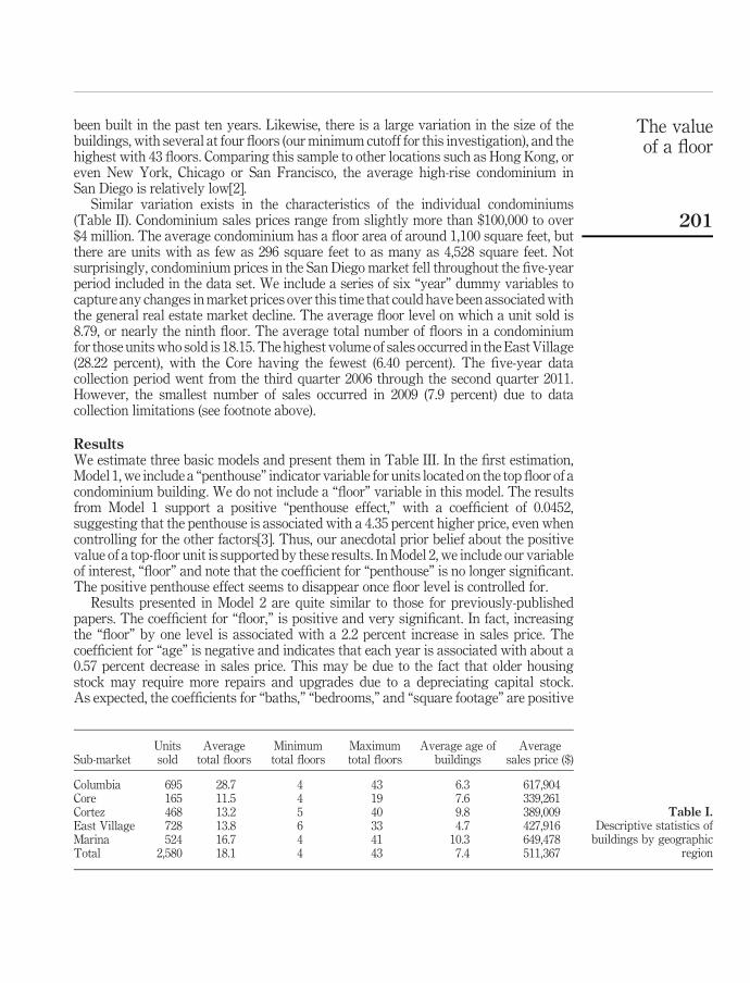
been built in the past ten years. Likewise, there is a large variation in the size of thebuildings, with several at four floors (our minimum cutoff for this investigation), and thehighest with 43 floors. Comparing this sample to other locations such as Hong Kong, oreven New York, Chicago or San Francisco, the average high-rise condominium inSan Diego is relatively low[2].

Similar variation exists in the characteristics of the individual condominiums(Table II). Condominium sales prices range from slightly more than $100,000 to over$4 million. The average condominium has a floor area of around 1,100 square feet, butthere are units with as few as 296 square feet to as many as 4,528 square feet. Notsurprisingly, condominium prices in the San Diego market fell throughout the five-yearperiod included in the data set. We include a series of six “year” dummy variables tocapture any changes in market prices over this time that could have been associated withthe general real estate market decline. The average floor level on which a unit sold is8.79, or nearly the ninth floor. The average total number of floors in a condominiumfor those units who sold is 18.15. The highest volume of sales occurred in the East Village(28.22 percent), with the Core having the fewest (6.40 percent). The five-year datacollection period went from the third quarter 2006 through the second quarter 2011.However, the smallest number of sales occurred in 2009 (7.9 percent) due to datacollection limitations (see footnote above).

ResultsWe estimate three basic models and present them in Table III. In the first estimation,Model 1, we include a “penthouse” indicator variable for units located on the top floor of acondominium building. We do not include a “floor” variable in this model. The resultsfrom Model 1 support a positive “penthouse effect,” with a coefficient of 0.0452,suggesting that the penthouse is associated with a 4.35 percent higher price, even whencontrolling for the other factors[3]. Thus, our anecdotal prior belief about the positivevalue of a top-floor unit is supported by these results. In Model 2, we include our variableof interest, “floor” and note that the coefficient for “penthouse” is no longer significant.The positive penthouse effect seems to disappear once floor level is controlled for.

Results presented in Model 2 are quite similar to those for previously-publishedpapers. The coefficient for “floor,” is positive and very significant. In fact, increasingthe “floor” by one level is associated with a 2.2 percent increase in sales price. Thecoefficient for “age” is negative and indicates that each year is associated with about a0.57 percent decrease in sales price. This may be due to the fact that older housingstock may require more repairs and upgrades due to a depreciating capital stock.As expected, the coefficients for “baths,” “bedrooms,” and “square footage” are positive

Sub-marketUnitssold

Averagetotal floors

Minimumtotal floors

Maximumtotal floors

Average age ofbuildings

Averagesales price ($)

Columbia 695 28.7 4 43 6.3 617,904Core 165 11.5 4 19 7.6 339,261Cortez 468 13.2 5 40 9.8 389,009East Village 728 13.8 6 33 4.7 427,916Marina 524 16.7 4 41 10.3 649,478Total 2,580 18.1 4 43 7.4 511,367

Table I.Descriptive statistics of

buildings by geographicregion

The valueof a floor

201

and significant. Specifically, an additional bathroom is associated with a 5.3 percentincrease in sales price, an additional bedroom with a 9.9 percent increase and a 100-foot increase in square footage is associated with about a 7.5 percent increase. Theneighborhood dummies are all negative and significant suggesting that there is anegative “neighborhood effect” vis-a-vis the reference category (Marina District). The“Core” neighborhood – in the central core of the CBD – has the largest negative“neighborhood effect” among those considered here. Perhaps this is due to a lack ofresidential amenities (e.g. grocery stores) available to residents in this sector of thecity. Sales occurring in 2006-2010 all seem to have had larger average sales prices,compared to 2011 (the reference category), with the largest effect in 2007. The regressionoverall explains approximately 87.5 percent of the variation in the dependent variable.

Variable Mean SD Minimum Maximum

Sales price $511,367 $338,431 $120,500 $4,250,000Ln sales price 12.99 0.523 11.70 15.26Age 7.36 9.54 1 82Baths 1.64 0.559 1 4Bedrooms 1.53 0.631 0 4Square footage 1,093.8 408.05 296 4,528Penthouse 0.088 0.283 0 1Floor 8.7 7.8 1 43Floor squared 139.5 254.1 1 1,849Relative floor 0.52 0.28 0.02326 1Total no. floors 18.14 11.99 4 43Columbia 0.26 0.44 0 1Core 0.06 0.24 0 1Cortez 0.18 0.38 0 1East village 0.28 0.45 0 1Marina 0.20 0.40 0 1Sale in Q2-2006 0.05 0.21 0 1Sale in Q3-2006 0.03 0.18 0 1Sale in Q4-2006 0.05 0.23 0 1Sale in Q1-2007 0.07 0.25 0 1Sale in Q2-2007 0.04 0.20 0 1Sale in Q3-2007 0.03 0.18 0 1Sale in Q4-2007 0.04 0.19 0 1Sale in Q1-2008 0.05 0.22 0 1Sale in Q2-2008 0.03 0.19 0 1Sale in Q3-2008 0.03 0.18 0 1Sale in Q4-2008 0.03 0.19 0 1Sale in Q1-2009 0.03 0.18 0 1Sale in Q4-2009a 0.04 0.20 0 1Sale in Q1-2010 0.05 0.21 0 1Sale in Q2-2010 0.06 0.25 0 1Sale in Q3-2010 0.06 0.24 0 1Sale in Q4-2010 0.04 0.21 0 1Sale in Q1-2011 0.06 0.24 0 1Sale in Q2-2011 0.07 0.25 0 1Sale in Q3-2011 0.05 0.23 0 1

Notes: n ¼ 2,580; asales data for Q2- and Q3-2009 were not available

Table II.Descriptive statistics forcondominium sales

IJHMA6,2

202

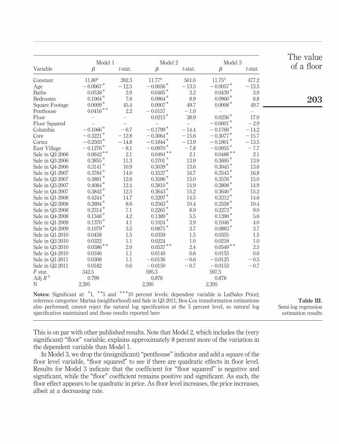
This is on par with other published results. Note that Model 2, which includes the (verysignificant) “floor” variable, explains approximately 8 percent more of the variation inthe dependent variable than Model 1.

In Model 3, we drop the (insignificant) “penthouse” indicator and add a square of thefloor level variable, “floor squared” to see if there are quadratic effects in floor level.Results for Model 3 indicate that the coefficient for “floor squared” is negative andsignificant, while the “floor” coefficient remains positive and significant. As such, thefloor effect appears to be quadratic in price. As floor level increases, the price increases,albeit at a decreasing rate.

Model 1 Model 2 Model 3Variable b t-stat. b t-stat. b t-stat.

Constant 11.80a 392.3 11.77a 501.0 11.75a 477.2Age 20.0067 * 212.5 20.0056 * 213.5 20.0057 * 213.5Baths 0.0538 * 2.9 0.0465 * 3.2 0.0439 * 3.0Bedrooms 0.1064 * 7.6 0.0964 * 8.9 0.0960 * 8.8Square Footage 0.0009 * 45.4 0.0007 * 49.7 0.0008 * 49.7Penthouse 0.0416 * * 2.2 20.0157 21.0 – –Floor – – 0.0215 * 38.9 0.0256 * 17.0Floor Squared – – – – 20.0001 * 22.9Columbia 20.1066 * 26.7 20.1799 * 214.4 20.1769 * 214.2Core 20.3221 * 212.8 20.3064 * 215.6 20.3077 * 215.7Cortez 20.2503 * 214.8 20.1844 * 213.9 20.1801 * 213.5East Village 20.1276 * 28.1 20.0970 * 27.8 20.0955 * 27.7Sale in Q2-2006 0.0642 * * 2.1 0.0494 * * 2.1 0.0488 * * 2.1Sale in Q3-2006 0.3855 * 11.3 0.3701 * 13.9 0.3695 * 13.9Sale in Q4-2006 0.3141 * 10.9 0.3039 * 13.6 0.3045 * 13.6Sale in Q1-2007 0.3784 * 14.0 0.3537 * 16.7 0.3543 * 16.8Sale in Q2-2007 0.3881 * 12.6 0.3596 * 15.0 0.3576 * 15.0Sale in Q3-2007 0.4084 * 12.4 0.3810 * 14.9 0.3808 * 14.9Sale in Q4-2007 0.3842 * 12.5 0.3643 * 15.2 0.3640 * 15.2Sale in Q1-2008 0.4244 * 14.7 0.3297 * 14.5 0.3312 * 14.6Sale in Q2-2008 0.2694 * 8.6 0.2563 * 10.4 0.2558 * 10.4Sale in Q3-2008 0.2314 * 7.1 0.2265 * 8.9 0.2273 * 9.0Sale in Q4-2008 0.1348 * 4.2 0.1389 * 5.5 0.1390 * 5.6Sale in Q1-2009 0.1370 * 4.1 0.1024 * 3.9 0.1046 * 4.0Sale in Q4-2009 0.1079 * 3.5 0.0875 * 3.7 0.0883 * 3.7Sale in Q1-2010 0.0458 1.5 0.0359 1.5 0.0355 1.5Sale in Q2-2010 0.0322 1.1 0.0224 1.0 0.0218 1.0Sale in Q3-2010 0.0586 * * 2.0 0.0537 * * 2.4 0.0549 * * 2.5Sale in Q4-2010 0.0346 1.1 0.0140 0.6 0.0155 0.6Sale in Q1-2011 0.0308 1.1 20.0136 20.6 20.0125 20.5Sale in Q2-2011 0.0182 0.6 20.0150 20.7 20.0153 20.7F stat. 342.5 595.3 597.5Adj R 2 0.799 0.878 0.878N 2,395 2,395 2,395

Notes: Significant at: *1, * *5 and * * *10 percent levels; dependent variable is Ln(Sales Price);reference categories: Marina (neighborhood) and Sale in Q3-2011; Box-Cox transformation estimationsalso performed; cannot reject the natural log specification at the 5 percent level, so natural logspecification maintained and those results reported here

Table III.Semi-log regression

estimation results

The valueof a floor

203

So far, the model specifications for estimating the impact of a floor level have onlyincluded “penthouse,” “floor” or “floor squared.” We wish to perform further tests inorder to see if the floor effect is monotonically increasing. To do this, we create apiecewise linear spline on the independent variable, “floor,” breaking the number offloors into five categories (1-4, 5-8, 9-12, 13-16 and 17-20 floors). These categories expressthe effect for the specific floor groupings compared to the reference category, namely,higher floors not explicitly controlled for in the model (Table IV).

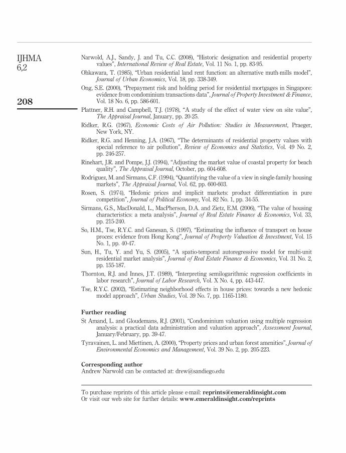
Results presented in Model 4 indicate that the lowest category (1-4 floors) has a largernegative effect on sales price (20.290) compared to the next category, 5-8 floors(20.224). These negative effects are in reference to the omitted category, floors higherthan the eighth floor[4]. Does this “lower-floor penalty” persist if we expand the model toinclude more categories? Results presented in Models 5 and 6 suggest that it does. InModel 6, the effect of a unit being located in the first four floors of a building is 20.461(compared to units located above 20 floors). This lower-floor penalty declinesmonotonically in magnitude to a value of20.146 for the units in floors 17-20. Comparingcoefficients for each of the categories, the change in magnitude of the penalty seems to belargest going from “floors 5-8” to “floors 9-12” (the coefficient falls in magnitude from20.395 to 20.270). Perhaps the ninth floor is just high enough to get a major shift in thetrade-off between the negative travel effect and the positive ambience effect. Thecoefficients for floor categories are shown in Figure 2.

ConclusionThis investigation has been an attempt to investigate the existence of a “higher-floorpremium” in condominiums in San Diego, California. In particular, we have attemptedto address two major shortcomings of prior investigations; namely that they havebeen rather narrow geographically (occurring largely in Southeast Asia) andmethodologically (including “floor” or “story” as a control, rather than a focus ofanalysis and without considering a separate “penthouse premium”).

Economic theory implies there may be two competing forces affecting the decisionto live on higher levels of a condominium building. On one hand, higher-level floors areassociated with longer travel times within a given building and hence higher implicittravel costs. However, there may also be positive amenities associated with livinghigher up such as less traffic noise, better views, etc.

Results presented here generally confirm those of prior investigations. Condominiumunits located on higher floors are associated with higher-sales prices, controlling for otherrelevant factors such as square footage, age, neighborhood and year sold. In other words,the positive ambience effect seems to dominate the higher travel costs associated with livingon higher floors. With very significant and positive coefficients for “floor” in Models 2 and 3(and their analogs in Models 4-6), our results support the existence of a higher-floorpremium. Specifically, we find that increasing floor level by one (at the mean) is associatedwith about a 2.2 percent increase in sales price. The floor level effect appears to be quadratic,with the coefficient for floor-squared negative and significant. Thus, higher floors areassociated with higher sales prices, though the increase occurs at a decreasing rate.

We do find some evidence for a “penthouse” effect in a simple model withoutcontrolling for “floor,” though the effect seems to disappear once we include “floor” inthe model. In other words, the top-floor does not seem to confer any additional valueover and above its advantage of being on a higher floor. When dividing the floors into

IJHMA6,2

204

categories, we find the coefficients for lower floor categories to be more negative thanthe floors in higher categories. Thus, the higher-floor premium appears to increasemonotonically from lower to higher floors. In addition, there appears to be a slightlylarger increase in the higher-floor premium moving from the 5-8 floors category to the

Model 4 Model 5 Model 6Variable b t-stat. b t-stat. b t-stat.

Constant 12.10a 341.1 12.14a 326.7 12.49a 281.9Age 20.0076 * 213.6 20.0064 * 211.3 20.0116 * 28.9Baths 0.0019 0.10 0.0369 * 1.7 20.0191 20.7Bedrooms 0.138 * 9.0 0.1221 * 6.9 0.1361 * 6.3Square footage 0.0008 * 43.7 0.0008 * 40.9 0.0007 * 36.0Floors 1-4 20.282 * 220.4 20.350 * 222.6 20.453 * 222.5Floors 5-8 20.2155 * 216.5 20.2823 * 219.4 20.3901 * 221.0Floors 9-12 – – 20.1713 * 210.4 20.2691 * 213.3Floors 13-16 – – – – 20.2006 * 29.5Floors 17-20 – – – – 20.1449 * 27.1Columbia 20.1770 * 210.8 20.1662 * 210.3 20.1605 * 29.2Core 20.3528 * 211.6 20.3210 * 210.8 – –Cortez 20.2501 * 212.7 20.2821 * 213.7 20.3092 * 213.4East village 20.1060 * 25.7 20.0535 * 22.8 20.1044 * 24.7Sale in Q2-2006 0.0332 1.0 0.0415 1.2 0.0116 0.35Sale in Q3-2006 0.3217 * 8.1 0.3257 * 8.3 0.2717 * 5.5Sale in Q4-2006 0.2719 * 8.0 0.2731 * 6.7 0.2818 * 5.8Sale in Q1-2007 0.3030 * 10.1 0.2859 * 9.4 0.2326 * 7.0Sale in Q2-2007 0.3017 * 9.0 0.2877 * 8.2 0.2635 * 7.2Sale in Q3-2007 0.3553 * 10.1 0.3408 * 9.6 0.3562 * 8.6Sale in Q4-2007 0.3455 * 11.0 0.3062 * 8.9 0.3105 * 8.3Sale in Q1-2008 0.3644 * 12.2 0.3534 * 11.6 0.3047 * 10.0Sale in Q2-2008 0.2377 * 7.2 0.2132 * 6.2 0.2620 * 7.2Sale in Q3-2008 0.2222 * 6.3 0.2325 * 6.3 0.2134 * 5.3Sale in Q4-2008 0.1052 * 3.1 0.1076 * 3.0 0.1703 * 4.3Sale in Q1-2009 0.1312 * 3.8 0.1330 * 3.6 0.1372 * 3.6Sale in Q4-2009 0.0995 * 3.0 0.1002 * 3.0 0.0906 * 2.6Sale in Q1-2010 0.0004 0.01 0.0027 0.08 0.0154 0.42Sale in Q2-2010 20.0163 20.56 20.0122 20.41 0.0084 0.25Sale in Q3-2010 0.0165 0.56 0.0135 0.45 0.0137 0.40Sale in Q4-2010 0.0208 0.66 0.0254 0.79 0.0024 0.07Sale in Q1-2011 20.0190 20.66 20.0223 20.75 20.0285 20.91Sale in Q2-2011 20.0076 20.27 20.0007 20.03 20.0158 20.54F stat. 332.08 316.54 215.09Adj. R 2 0.8493 0.8636 0.8646n 1,704 1,496 1,040

Notes: Significant at: *1, * *5 and * * *10 percent levels; dependent variable is Ln(Sales Price);reference categories: all floors higher than the highest spline specification in each model, e.g. forModel 4, all floors higher than eighth floor are reference category; Marina (neighborhood); and Sale inQ3-2011; Box-Cox transformation estimations also performed; cannot reject the natural logspecification at the 5 percent significance level for Model 4; however, no coefficients changed signs orrelative magnitude and only one (Bathrooms) changed significance levels (increased in significance to5 percent level); cannot reject the natural log specification at the 5 percent significance level for Models5 or 6 so natural log specification reported here

Table IV.Semi-log regression

estimation results withfloor dummies

The valueof a floor

205

9-12 floors category. We speculate that this could be a transition point where thepositive ambience effect dominates much more than the negative travel cost effect(moving up from the 5-8 floors to the 9-12 floors category).

While we control for a number of factors affecting sales price and our adjusted R 2

values are in line with other published reports in this area, data limitations preventedus from considering other factors such as noise level (Brandt and Maennig, 2011),average elevator speeds and ocean views (Rodriguez and Sirmans, 1994; Benson et al.,1998). An additional limitation of this study is that San Diego’s high-rise condominiummarket may be lower on average than some other large cities, which could limit thegeneralizability of this study. We leave these and other issues for future research.

Notes

1. Due to data limitations, we were unable to obtain data for the third and fourth quarters of2009, though we do not expect those omissions to affect our results. While there were 2,580condominium sales in the data set, missing values for some of the observations resulted in2,395 observations used in the regression estimations.

2. However, our mean number of floors is similar to the mean reported for the two Singaporestudies referenced above.

3. We interpret the coefficients from the semi-log estimations following Thornton and Innes(1989, p. 444), who suggest that “to calculate the true proportional change in Y resulting from anon-infinitesimal change in X, one would have to calculate: g ¼ exp(bDX) – 1.” See also,Halvorsen and Palmquist (1980) for a related discussion on interpretation of dummy variables.

4. Only observations for which there were more than eight floors were included in thisestimation, which is why the number of observations has fallen to 898.

References

Asabere, P.K. and Huffman, F.E. (2009), “The relative impacts of trails and greenbelts on homeprice”, Journal of Real Estate Finance & Economics, Vol. 38 No. 4, pp. 408-419.

Baranzini, A. and Schaerer, C. (2011), “A sight for sore eyes: assessing the value of view and land usein the housing market”, Journal of Housing Economics, Vol. 20 No. 3, pp. 191-199.

Figure 2.Coefficient for floorcategories, 1-4 through17-20

0

–0.05

–0.1

–0.15

1-4 5-8 9-12 13-16 17-20

–0.2

–0.25C

oef

fici

ent

–0.3

–0.35

–0.4

–0.45

–0.5Floor categories

IJHMA6,2

206

Benson, E.D., Hansen, J.L., Schwartz, A.L. Jr and Smersh, G.T. (1998), “Pricing residential amenities:the value of a view”, Journal of Real Estate Finance & Economics, Vol. 16 No. 1, pp. 55-73.

Blackley, P., Follain, J.R. Jr and Ondrich, J. (1984), “Box-cox estimation of hedonic models: howserious is the iterative OLS variance biase?”, Review of Economics and Statistics, Vol. 66No. 2, pp. 348-353.

Brandt, S. and Maennig, W. (2011), “Road noise exposure and residential property prices:evidence from Hamburg”, Transportation Research Part D, Vol. 16, pp. 23-30.

Chau, K.W. and Ng, F.F. (1998), “The effects of improvement in public transportation capacity onresidential price gradient in Hong Kong”, Journal of Property Valuation & Investment,Vol. 16 No. 4, pp. 397-410.

Chau, K.W., Ma, V.S.M. and Ho, D.C.W. (2001), “The pricing of the ‘luckiness’ in the apartmentmarket”, Journal of Real Estate Literature, Vol. 9 No. 1, pp. 31-40.

Chau, K.W., Leung, A.Y.T., Yiu, C.Y. and Wong, S.K. (2003), “Estimating the value enhancementeffects of refurbishment”, Facilities, Vol. 21 Nos 1/2, pp. 13-19.

Chin, T.L., Chau, K.W. and Ng, F.F. (2004), “The impact of the Asian financial crisis on the pricing ofcondominiums in Malaysia”, Journal of Real Estate Literature, Vol. 12 No. 1, pp. 33-49.

Colwell, P.F. and Sirmans, C.F. (1978), “Area, time, centrality and the value of urban land”, LandEconomics, Vol. 54 No. 4, pp. 514-519.

Conroy, S.J. and Milosch, J.L. (2011), “An estimation of the coastal premium for residentialhousing prices in San Diego county”, Journal of Real Estate Finance & Economics, Vol. 42No. 2, pp. 211-228.

Conway, D., Li, C.Q., Wolch, J., Kahle, C. and Jerrett, M. (2010), “A spatial autocorrelationapproach for examining the effects of urban greenspace on residential property values”,Journal of Real Estate Finance & Economics, Vol. 41 No. 2, pp. 150-169.

Coulson, N.E. and Engle, R.F. (1987), “Transportation costs and the rent gradient”, Journal ofUrban Economics, Vol. 21, pp. 287-297.

Cropper, M.L., Deck, L.B. and McConnell, K.E. (1988), “On the choice of functional form for hedonicprice functions”, Review of Economic and Statistics, Vol. 70 No. 4, pp. 668-675.

Halvorsen, R. and Palmquist, R. (1980), “The interpretation of dummy variables insemilogarithmic equations”, American Economic Review, Vol. 3, pp. 474-475.

Irwin, E.G. (2002), “The effects of open space on residential property values”, Land Economics,Vol. 78 No. 4, pp. 465-480.

Kau, J.B. and Sirmans, C.F. (1979), “Urban land value functions and the price elasticity of demandfor housing”, Journal of Urban Economics, Vol. 6, pp. 112-121.

Kilpatrick, J.A., Throupe, R.L., Carruthers, J.I. and Krause, A. (2007), “The impact of transit corridorson residential property values”, Journal of Real Estate Research, Vol. 29 No. 3, pp. 303-320.

Mahan, B.L., Polasky, S. and Adams, R.M. (2000), “Valuing urban wetlands: a property priceapproach”, Land Economics, Vol. 76 No. 1, pp. 100-113.

Major, C. and Lusht, K.M. (2004), “Beach proximity and the distribution of property values inshore communities”, The Appraisal Journal, Fall, pp. 333-338.

Mills, E.S. (1972), Urban Economics, Scott Foresman, Glenview, IL.

Mok, H.M.K., Chan, P.P.K. and Cho, Y.S. (1995), “A hedonic price model for private properties inHong Kong”, Journal of Real Estate Finance & Economics, Vol. 10, pp. 37-48.

Muth, R.F. (1969), Cities and Housing; The Spatial Pattern of Urban Residential Land Use,University of Chicago Press, Chicago, IL.

The valueof a floor

207

Narwold, A.J., Sandy, J. and Tu, C.C. (2008), “Historic designation and residential propertyvalues”, International Review of Real Estate, Vol. 11 No. 1, pp. 83-95.

Ohkawara, T. (1985), “Urban residential land rent function: an alternative muth-mills model”,Journal of Urban Economics, Vol. 18, pp. 338-349.

Ong, S.E. (2000), “Prepayment risk and holding period for residential mortgages in Singapore:evidence from condominium transactions data”, Journal of Property Investment & Finance,Vol. 18 No. 6, pp. 586-601.

Plattner, R.H. and Campbell, T.J. (1978), “A study of the effect of water view on site value”,The Appraisal Journal, January, pp. 20-25.

Ridker, R.G. (1967), Economic Costs of Air Pollution: Studies in Measurement, Praeger,New York, NY.

Ridker, R.G. and Henning, J.A. (1967), “The determinants of residential property values withspecial reference to air pollution”, Review of Economics and Statistics, Vol. 49 No. 2,pp. 246-257.

Rinehart, J.R. and Pompe, J.J. (1994), “Adjusting the market value of coastal property for beachquality”, The Appraisal Journal, October, pp. 604-608.

Rodriguez, M. and Sirmans, C.F. (1994), “Quantifying the value of a view in single-family housingmarkets”, The Appraisal Journal, Vol. 62, pp. 600-603.

Rosen, S. (1974), “Hedonic prices and implicit markets: product differentiation in purecompetition”, Journal of Political Economy, Vol. 82 No. 1, pp. 34-55.

Sirmans, G.S., MacDonald, L., MacPherson, D.A. and Zietz, E.M. (2006), “The value of housingcharacteristics: a meta analysis”, Journal of Real Estate Finance & Economics, Vol. 33,pp. 215-240.

So, H.M., Tse, R.Y.C. and Ganesan, S. (1997), “Estimating the influence of transport on houseproces: evidence from Hong Kong”, Journal of Property Valuation & Investment, Vol. 15No. 1, pp. 40-47.

Sun, H., Tu, Y. and Yu, S. (2005), “A spatio-temporal autoregressive model for multi-unitresidential market analysis”, Journal of Real Estate Finance & Economics, Vol. 31 No. 2,pp. 155-187.

Thornton, R.J. and Innes, J.T. (1989), “Interpreting semilogarithmic regression coefficients inlabor research”, Journal of Labor Research, Vol. X No. 4, pp. 443-447.

Tse, R.Y.C. (2002), “Estimating neighborhood effects in house prices: towards a new hedonicmodel approach”, Urban Studies, Vol. 39 No. 7, pp. 1165-1180.

Further reading

St Amand, L. and Gloudemans, R.J. (2001), “Condominium valuation using multiple regressionanalysis: a practical data administration and valuation approach”, Assessment Journal,January/February, pp. 39-47.

Tyravainen, L. and Miettinen, A. (2000), “Property prices and urban forest amenities”, Journal ofEnvironmental Economics and Management, Vol. 39 No. 2, pp. 205-223.

Corresponding authorAndrew Narwold can be contacted at: drew@sandiego.edu

IJHMA6,2

208

To purchase reprints of this article please e-mail: reprints@emeraldinsight.comOr visit our web site for further details: www.emeraldinsight.com/reprints