The Use of Oligopoly Equilibrium

for Economic and Policy Applications

Jim Bushnell, UC Energy Institute and Haas School of Business

A Dual Mission

• “Research Methods” - how oligopoly models can be used to tell us something useful about how markets work– Potentially very boring

• What makes electricity markets work (or not)?– Blackouts, Enron, “manipulation,” etc.– A new twist on how we think about vertical

relationships– Potentially very exciting

Oligopoly Models

– Large focus on theoretical results– Simple oligopoly models provide the

“structure” for structural estimation in IO

– Seldom applied to large data sets of complex markets• Some markets feature a wealth of detailed

data• Optimization packages make calculation of

even complex equilibria feasible

A Simple Oligopoly Model

• Concentration measures

where m is Cournot equilibrium margin.

HHI s i2

i

qi

Q

2

i

m p MC

p

1

n

HHI

Surprising Fact: Oligopoly models can tell us

something about reality• Requires careful consideration about the

institutional details of the market environment – Incentives of firms (Fringe vs. Oligopoly)– Physical aspects of production (transmission)– Vertical & contractual arrangements

• Recent research shows actual prices in several electricity markets reasonably consistent with Cournot prices

• Cournot models don’t have to be much more complicated than HHI calculations

b

nqap

bcn

bkaq i

i

,1

Empirical Applications

• Analysis of policy proposals– Prospective analysis of future market– Merger review, market liberalization, etc.

• Market-level empirical analysis– Retrospective analysis of historic market– Diagnose sources of competition problems– Simulate potential solutions

• Firm-level empirical analysis– Estimate costs or other parameters (contracts)– Evaluate optimality of firm’s “best” response– Potentially diagnose collusive outcomes

Oligopoly equilibrium models

• Cournot – firms set quantities– many variations

• Supply-function – firms bid p-q pairs– infinite number of functional forms– Range of potential outcomes is bounded by

Cournot and competitive– Capacity constraints, functional form

restrictions reduce the number of potential equilibria

• Differentiated products models (Bertrand)

Green and Newbery (1992)

Simple Example

• 2 firms, c(q) = 1/2 qi 2, c = mc(q) = qi

• Market supply = Q = q1 + q2

• Linear demand Q = a-b*p = 10 – p• NO CAPACITY CONSTRAINTS

3

10

2)(

0)2(

5.)( 2

jjiji

iji

i

i

iiji

i

q

b

qaqqBR

qb

qqa

q

qqb

qqa

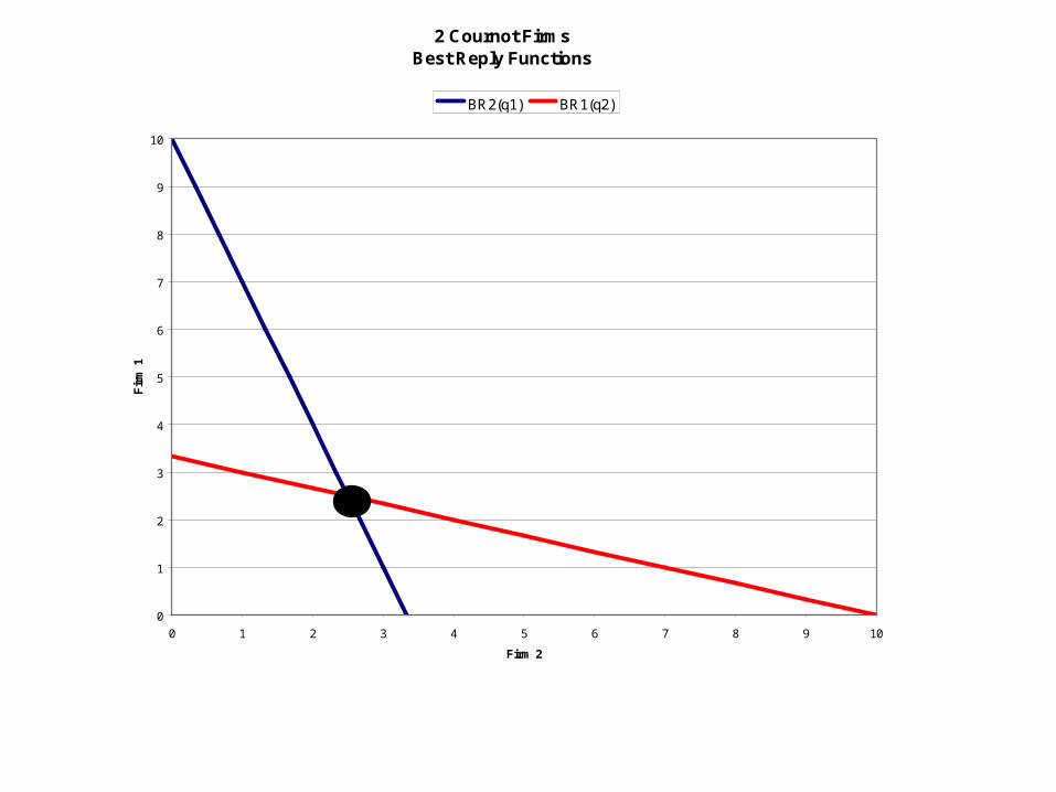
2 Cournot FirmsBest Reply Functions

0

1

2

3

4

5

6

7

8

9

10

0 1 2 3 4 5 6 7 8 9 10

Firm 2

Fir

m 1

BR2(q1) BR1(q2)

Three Studies of Electricity

• Non-incremental regulatory and structural changes– Historic data not useful for predicting future behavior

• Large amounts of cost and market data available– High frequency data - legacy of regulation

• Borenstein and Bushnell (1999)– Simulation of prospective market structures

• Focus on import capacity constraints

• Bushnell (2005)– Simulation using actual market conditions

• Focus on import elasticities

• Bushnell, Saravia, and Mansur (2006)– Simulation of several markets

12

Western Regional Markets

• Path from NW to northern California rated at 4880 MW

• Path from NW to southern California rated at 2990 MW

• Path from SW to southern California rated at 9406 MW (W-O-R constraint)

• 408 MW path from northern Mexico and 1920 MW path from Utah

13

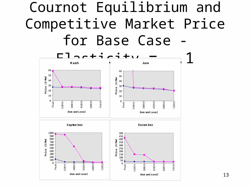
Cournot Equilibrium andCompetitive Market Price for Base Case - Elasticity = -.1

March

0

10

20

30

40

50

60

Pe

ak

15

0th

30

0th

45

0th

60

0th

74

4th

Demand Level

Pri

ce

($

/Mw

h)

June

0

10

20

30

40

50

60

Pe

ak

15

0th

30

0th

45

0th

60

0th

72

0th

Demand Level

Pri

ce

($

/Mw

h)

September

0100200300400500600700800900

1000

Pe

ak

15

0th

30

0th

45

0th

60

0th

72

0th

Demand Level

Pri

ce

($

/Mw

h)

December

050

100150200250300350400450500

Pe

ak

15

0th

30

0th

45

0th

60

0th

74

4th

Demand Level

Pri

ce

($

/Mw

h)

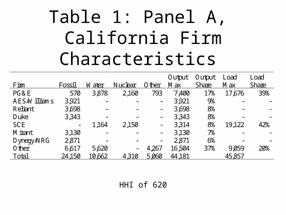
Table 1: Panel A, California Firm Characteristics

HHI of 620

Output Output Load Load Firm Fossil Water Nuclear Other Max Share Max Share PG&E 570 3,878 2,160 793 7,400 17% 17,676 39% AES/Williams 3,921 - - - 3,921 9% - - Reliant 3,698 - - - 3,698 8% - - Duke 3,343 - - - 3,343 8% - - SCE - 1,164 2,150 - 3,314 8% 19,122 42% Mirant 3,130 - - - 3,130 7% - - Dynegy/NRG 2,871 - - - 2,871 6% - - Other 6,617 5,620 - 4,267 16,504 37% 9,059 20% Total 24,150 10,662 4,310 5,060 44,181 45,857

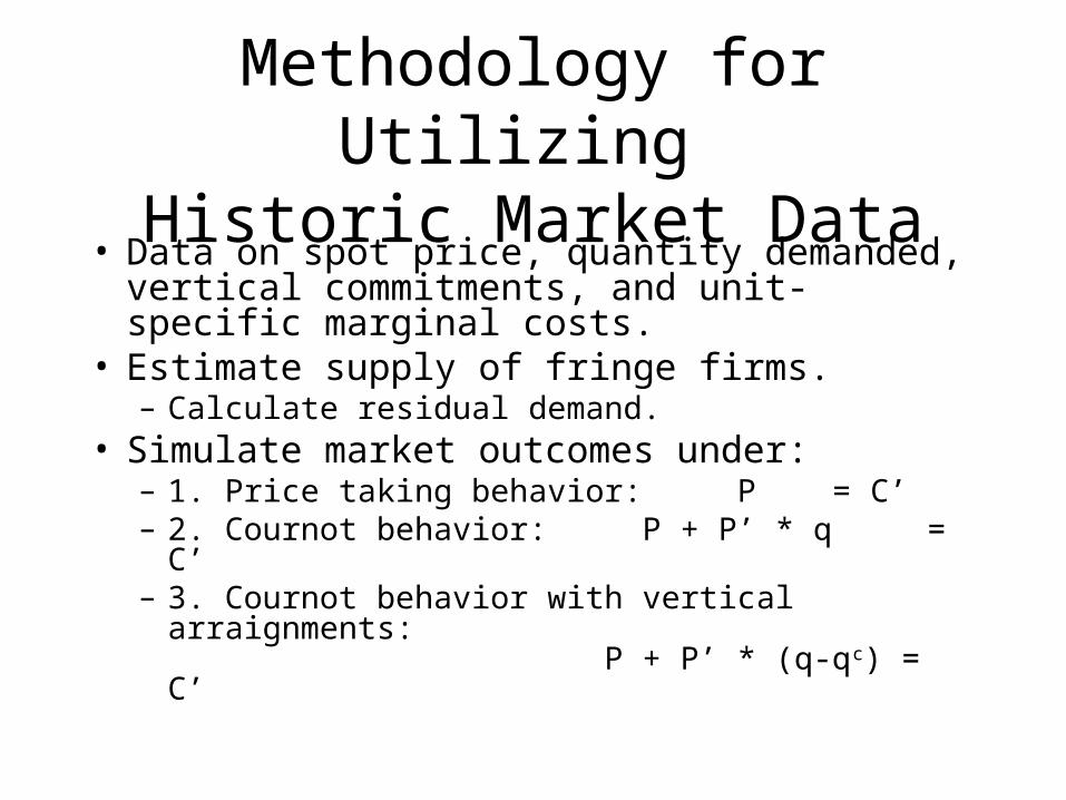
Methodology for Utilizing Historic Market Data

• Data on spot price, quantity demanded, vertical commitments, and unit-specific marginal costs.

• Estimate supply of fringe firms.– Calculate residual demand.

• Simulate market outcomes under:– 1. Price taking behavior: P =

C’– 2. Cournot behavior: P + P’ * q = C’– 3. Cournot behavior with vertical

arraignments: P + P’ * (q-qc) = C’

Modeling Imports and Fringe

• Source of elasticity in model• We observe import quantities, market price, and weather

conditions in neighboring states• Estimate the following regression using 2SLS (load as

instrument)

9

6 1

7 24

2 2

ln( )S

fringet i it t s st

i s

j jt h ht tj h

q Month p Temp

Day Hour

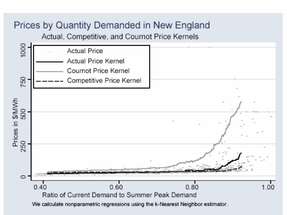
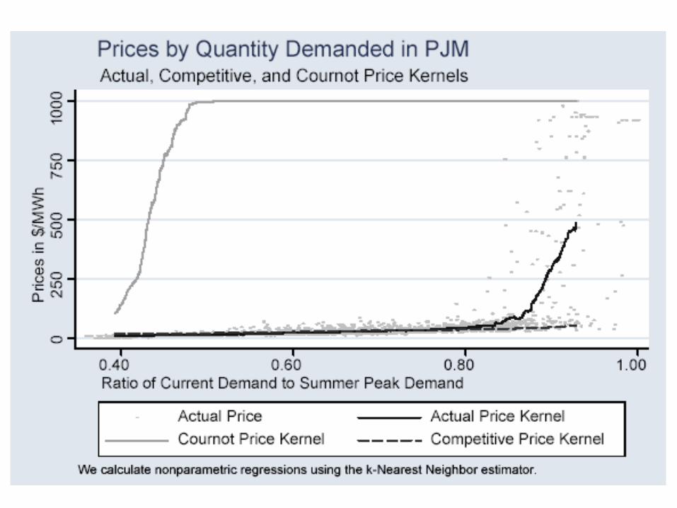
• Estimates of price responsiveness are greatest in California (>5000) relative to New England (1250) and PJM (850)

Residual Demand function

ttt

actualt

actualtt

Qp

pQ

exp

)ln(

• The demand curve is fit through the observed price and quantity outcomes.

mean mean meanobservations Cournot PX Competitive

price ($/MWh) price ($/MWh) price ($/MWh)June 699 127.93 122.29 52.67July 704 131.84 108.60 60.27August 724 185.02 169.16 79.14September 696 116.26 116.64 75.12

Table 1: Cournot Simulation and Actual PX Prices - Summer 2000

Simulation ResultsCalifornia 2000

01

00

20

03

00

40

0co

urn

ot/

PX

_p

rice

/co

mp

etit

ive

0 5000 10000 15000dem_cal

cournot PX_price

competitive

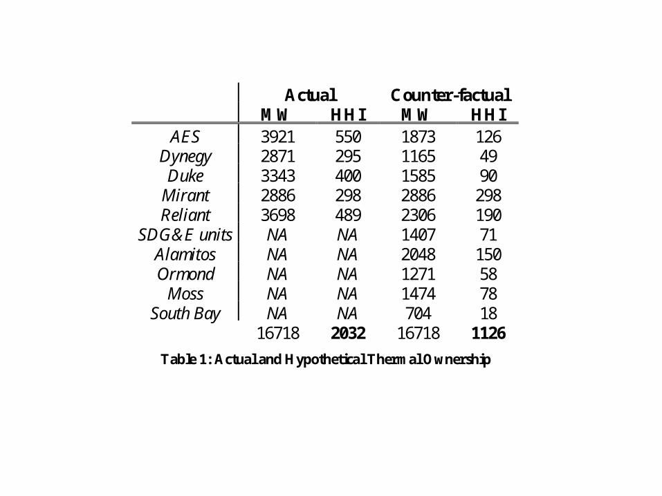
Actual Counter-factualMW HHI MW HHI

AES 3921 550 1873 126Dynegy 2871 295 1165 49Duke 3343 400 1585 90

Mirant 2886 298 2886 298Reliant 3698 489 2306 190

SDG&E units NA NA 1407 71Alamitos NA NA 2048 150Ormond NA NA 1271 58

Moss NA NA 1474 78South Bay NA NA 704 18

16718 2032 16718 1126

Table 1: Actual and Hypothetical Thermal Ownership

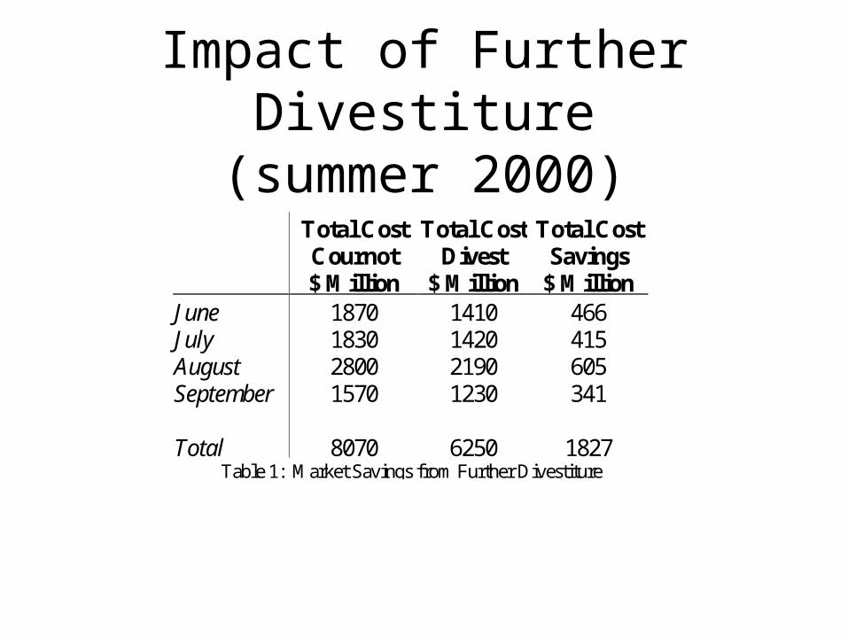
Total Cost Total Cost Total CostCournot Divest Savings$ Million $ Million $ Million

June 1870 1410 466July 1830 1420 415August 2800 2190 605September 1570 1230 341

Total 8070 6250 1827Table 1: Market Savings from Further Divestiture

Impact of Further Divestiture

(summer 2000)

September 2000 Cournot Prices

0.00

50.00

100.00

150.00

200.00

250.00

300.00

0 2000 4000 6000 8000 10000 12000 14000 16000 18000

Residual Demand

Pri

ce (

$/M

Wh

)

Simple Cournot actual non-linear cournot

The Effect of Forward Contracts

• Contract revenue is sunk by the time the spot market is run– no point in withholding output to drive up a price

that is not relevant to you• More contracts by 1 firm lead to more spot

production from that firm, less from others• More contracts increase total production

– lower prices• Firms would like to be the only one signing

contracts, are in trouble if they are the only ones not signing contracts– prisoner’s dilemma

Simple Example

– 2 firms, c(q) = 1/2 qi 2, c = mc(q) = qi

– Market supply = Q = q1 + q2

– Linear demand Q = a-b*p = 10 – p– NO CAPACITY CONSTRAINTS

– Firm 2 has contracts for quantity qc2

3

10

2)(

0)2(

5.)(

2121212

2212

2

2

2222

122

cc

c

c

qq

b

qqaqqBR

qb

qqqa

q

qqqb

qqa

2 Cournot FirmsBest Reply Functions

0

1

2

3

4

5

6

7

8

9

10

0 1 2 3 4 5 6 7 8 9 10

Firm 2

Fir

m 1

BR2(q1) BR1(q2)

2 Cournot FirmsBest Reply Functions

0

1

2

3

4

5

6

7

8

9

10

0 1 2 3 4 5 6 7 8 9 10

Firm 2

Fir

m 1

BR2(q1) BR1(q2)

Green and Newbery (1992)

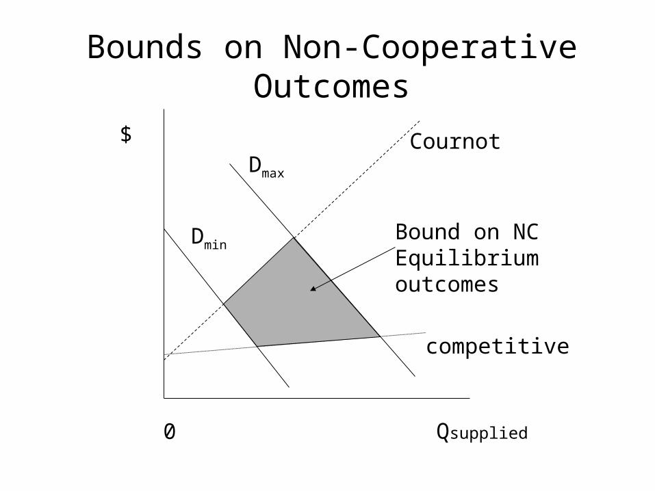
0

$Dmax

DminBound on NCEquilibriumoutcomes

Cournot

competitive

Bounds on Non-Cooperative Outcomes

Qsupplied

0

$

Qsupplied

Dmax

DminBound on NCEquilibriumoutcomes

Cournot

competitive

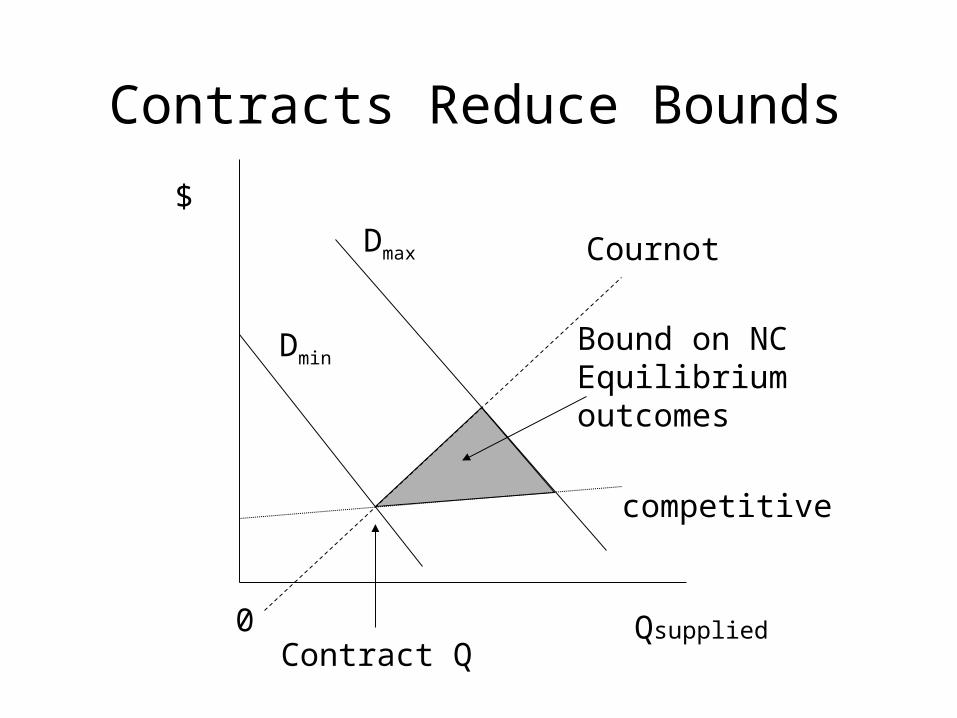
Contracts Reduce Bounds

Contract Q

0

Dmax

Dmin Bound on NCEquilibriumoutcomes

Cournot

competitive

Contract QQsupplied

$

“Over-Contracting’ can drive prices below competitive

levels

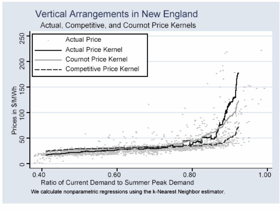
Vertical structure and forward commitments

• Vertical integration makes a firm a player in two serially related markets

• Usually we think of wholesale (upstream) price determining the (downstream) retail price– Gilbert and Hastings– Hendricks and McAfee (simultaneous)

• In some markets, retailers make forward commitments to customers– utilities – telecom services – construction

• In these markets a vertical arrangement plays the same role as a forward contract– a pro-competitive effect

Retail and Generation in PJM, 1999

GPU Inc.GPU Inc.

Public Service Electric & Gas

Public Service Electric & Gas

PECO Energy

PECO EnergyPP&L Inc.

PP&L Inc.

Potomac Electric Power

Potomac Electric Power

Baltimore Gas & Electric

Baltimore Gas & ElectricOther

Other

0%

10%

20%

30%

40%

50%

60%

70%

80%

90%

100%

Retail Generation

Retail and Generation in New England 1999

Northeast Util.Northeast Util.

PG&E N.E.G.

PG&E N.E.G.

Mirant

Sithe

FP&L Energy

Wisvest

Other

Other

0%

10%

20%

30%

40%

50%

60%

70%

80%

90%

100%

Retail Generation

Retail and Generation in California 1999

PG&E

PG&E

SCE

SCE

AES/Williams

Reliant

Mirant

Duke

Dynegy/NRG

Other

Other

0%

10%

20%

30%

40%

50%

60%

70%

80%

90%

100%

Retail Generation

Methodology

• Simulate prices under:– Price taking behavior– Cournot behavior– Cournot with vertical arraignments (integration or

contracts)

, c tt i,t -i,t i,t i,t i,t i,t

, i,t

p=p (q ,q )+[q -q ]· -C (q ) 0

qi t

i tq

ci,tq

• Use market data on spot price, market demand and production costs.

• The first order condition is:

Methodology

• Data on spot price, quantity demanded, vertical commitments, and unit-specific marginal costs.

• Estimate supply of fringe firms.– Calculate residual demand.

• Simulate market outcomes under:– 1. Price taking behavior: P = C’– 2. Cournot behavior: P + P’ * q = C’– 3. Cournot behavior with vertical arraignments:

P + P’ * (q-qc) = C’

Summary

• Oligopoly models married with careful empirical methods are a useful tool for both prospective and retrospective analysis of markets

• Careful consideration of the institutional details of the market is necessary

• In electricity, vertical arrangements (or contracts) appear to be a key driver of market performance– The form and extent of these arrangements going

forward will determine whether the “success” of the markets that are working well can be sustained