The total differential - Georg-August-Universität Göttingenwkurth/csm14_v08.pdf · The total...
65
1 The total differential The total differential of the function of two variables The total differential gives the full information about rates of change of the function in the -direction and in the -direction.
Transcript of The total differential - Georg-August-Universität Göttingenwkurth/csm14_v08.pdf · The total...

1
The total differential
The total differential of the function of two variables ��
The total differential gives the full information about rates of change of the function in the �-direction and in the �-direction.
�� � ���� �� � ���� ��
2
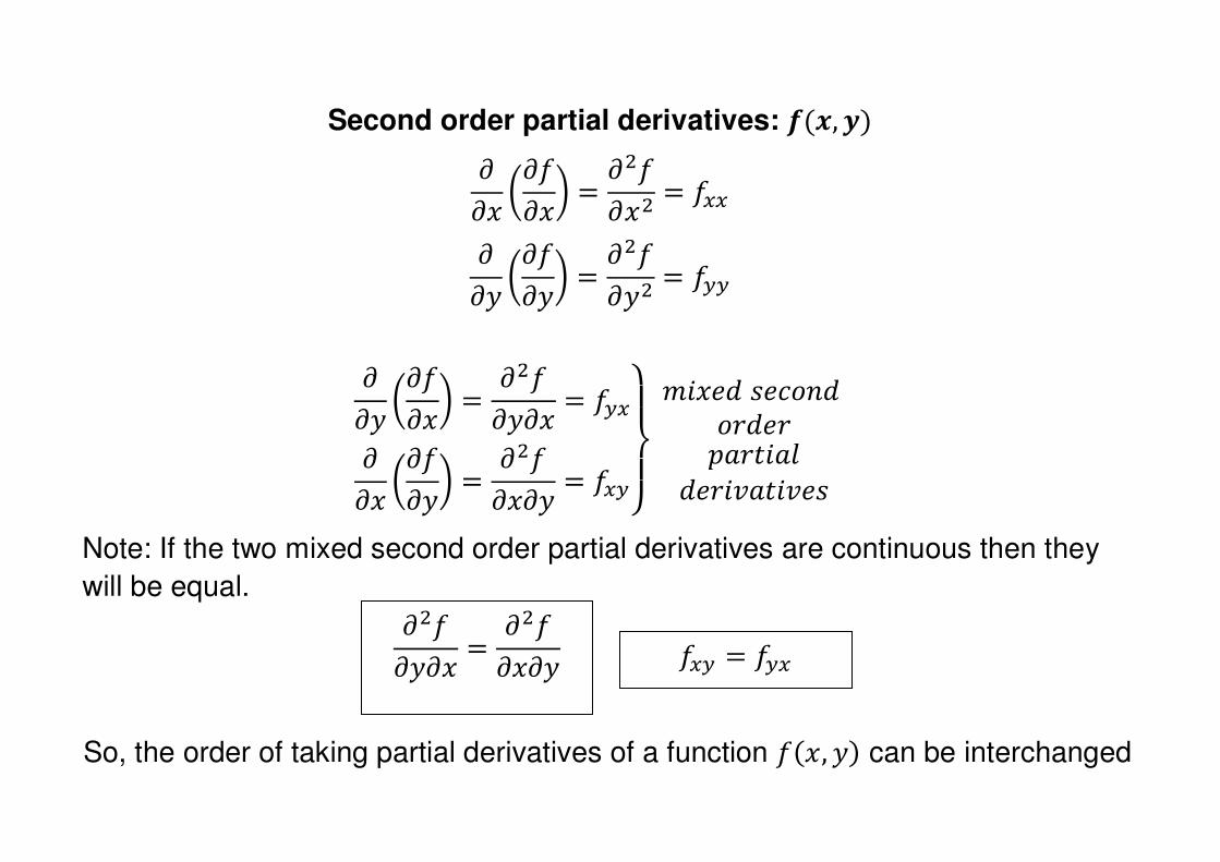
Second order partial derivatives: �, � ��� ������ � ������ � ���
��� ������ � ������ � ���
���� ������ � ������� � ������ ������ � ������� � ������
�� ����� ������ � �� !" #�"$�� �%"#�%��
Note: If the two mixed second order partial derivatives are continuous then they
will be equal.
������� � ������� ��� � ���
So, the order of taking partial derivatives of a function ��, �� can be interchanged
3
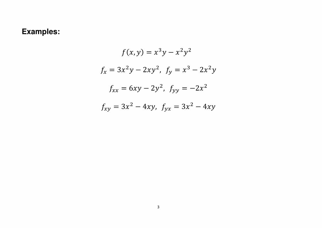
Examples:
��, �� � �&� ' ���� �� � 3��� ' 2���, �� � �& ' 2���
��� � 6�� ' 2��, ��� � '2��
��� � 3�� ' 4��, ��� � 3�� ' 4��
4
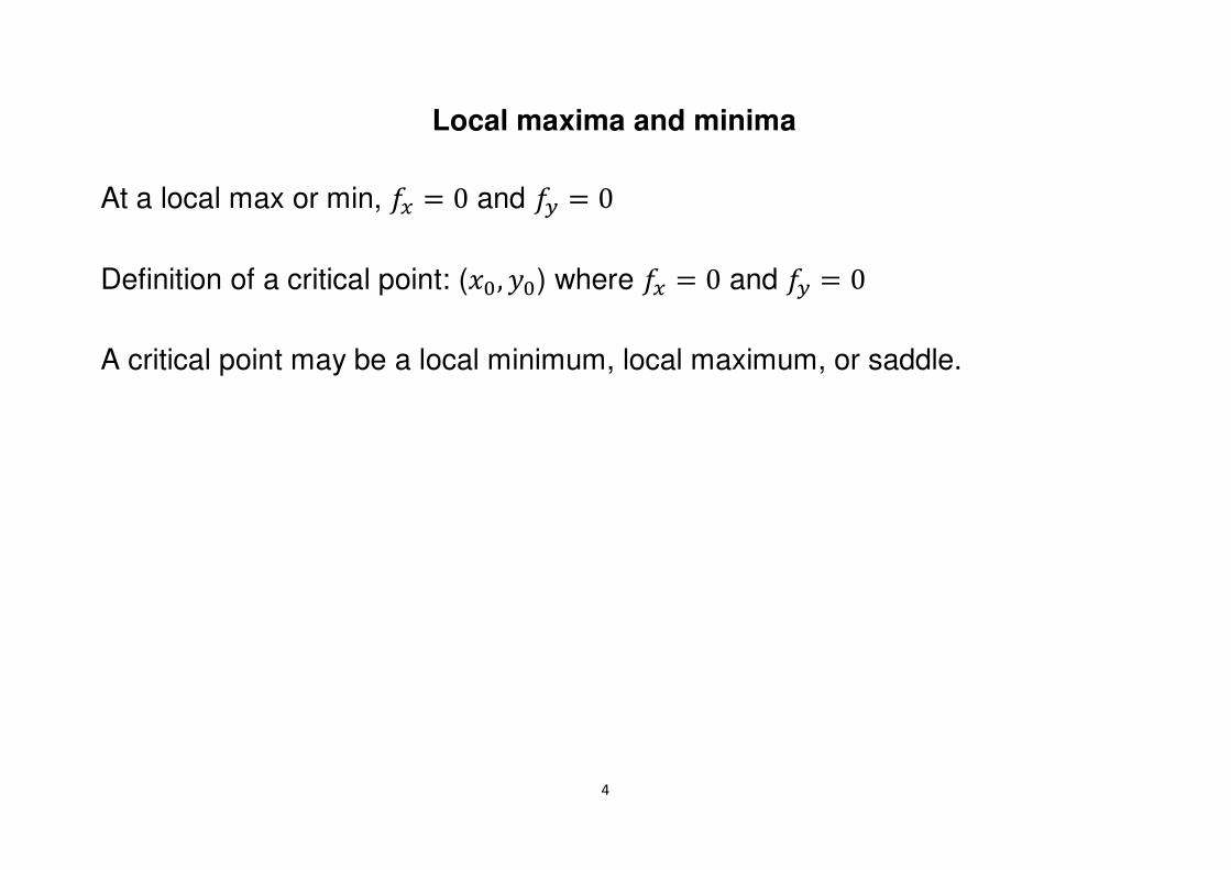
Local maxima and minima
At a local max or min, �� � 0 and �� � 0
Definition of a critical point: (�-, �-) where �� � 0 and �� � 0
A critical point may be a local minimum, local maximum, or saddle.
5
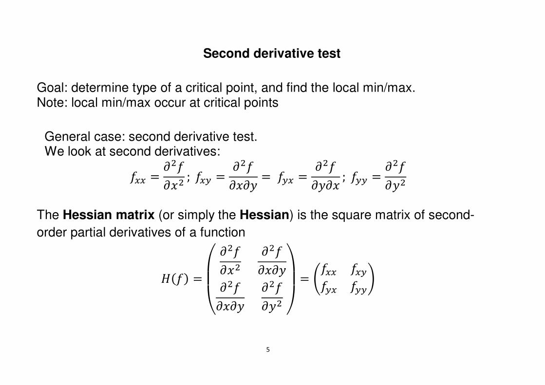
Second derivative test
Goal: determine type of a critical point, and find the local min/max. Note: local min/max occur at critical points
General case: second derivative test. We look at second derivatives:
��� � ������ ; ��� � ������� � ��� � ������� ; ��� � ������
The Hessian matrix (or simply the Hessian) is the square matrix of second-
order partial derivatives of a function /�� �
012
������ �������������� ������ 345 � 6��� ������ ���7

6
Given is � and a critical point �-, �-�.
Define the second derivative test discriminant as
8 � ����-, �-� · ����-, �-� ' ����-, �-� · ����-, �-�
Then
local minimum
local maximum
If 8 : 0 and ����-, �-� : 0
saddle
cannot be concluded
If 8 : 0 and ����-, �-� ; 0
If 8 ; 0
If 8 � 0
7
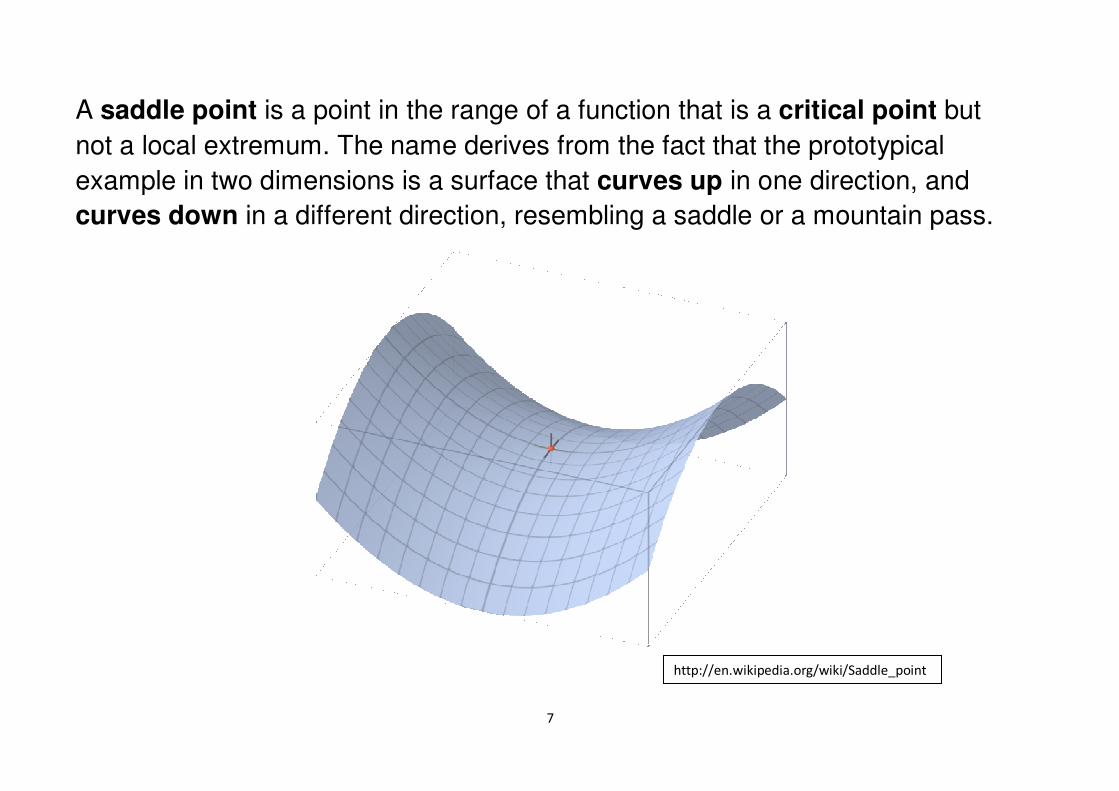
A saddle point is a point in the range of a function that is a critical point but
not a local extremum. The name derives from the fact that the prototypical
example in two dimensions is a surface that curves up in one direction, and
curves down in a different direction, resembling a saddle or a mountain pass.
http://en.wikipedia.org/wiki/Saddle_point

8
Example:
��, �� � �& � ��� � 1� ' 12� � 11
�� � � � 1�2� �� � 3�� � �� ' 12
��� � 2� � 2 ��� � 6� ��� � ��� � 2�
Critical points candidates: First derivative test applied
�� � � � 1�2� � 0 �� � 3�� � �� ' 12 � 0
We need to solve the following system of equations:
= � � 1�2� � 03�� � �� ' 12 � 0� The critical points are:
�>, �>� � 3, '1� ; ��, ��� � '3, '1�; �&, �&� � 0, '2� ; �?, �?� � 0,2�
9
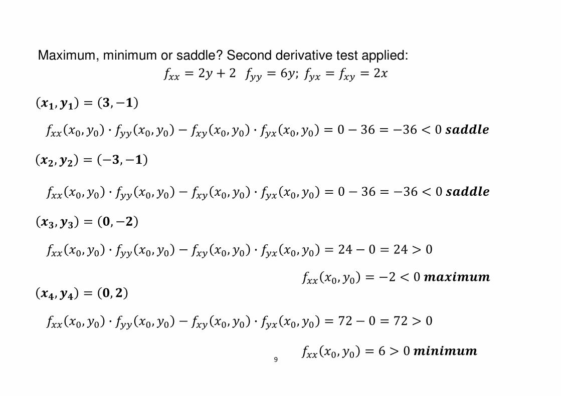
Maximum, minimum or saddle? Second derivative test applied: ��� � 2� � 2 ��� � 6�; ��� � ��� � 2�
�@, @� � A, '@�
����-, �-� · ����-, �-� ' ����-, �-� · ����-, �-� � 0 ' 36 � '36 ; 0 BCDDEF
�G, G� � 'A, '@�
����-, �-� · ����-, �-� ' ����-, �-� · ����-, �-� � 0 ' 36 � '36 ; 0 BCDDEF
�A, A� � H, 'G�
����-, �-� · ����-, �-� ' ����-, �-� · ����-, �-� � 24 ' 0 � 24 : 0
����-, �-� � '2 ; 0 IC�JIKI �L, L� � H, G�
����-, �-� · ����-, �-� ' ����-, �-� · ����-, �-� � 72 ' 0 � 72 : 0
����-, �-� � 6 : 0 IJNJIKI
10
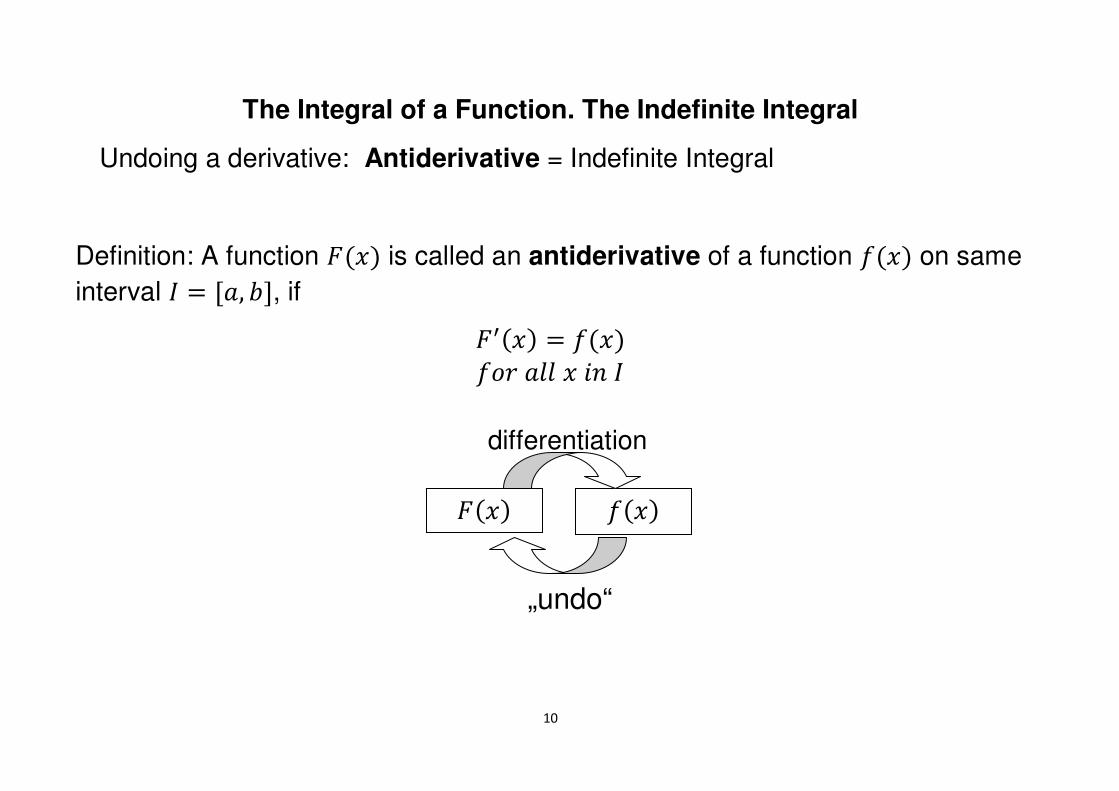
The Integral of a Function. The Indefinite Integral
Undoing a derivative: Antiderivative = Indefinite Integral
Definition: A function O�� is called an antiderivative of a function ��� on same
interval P � Q", RS, if OT�� � ����� "$$ � �� P
O�� ���
differentiation
„undo“
11
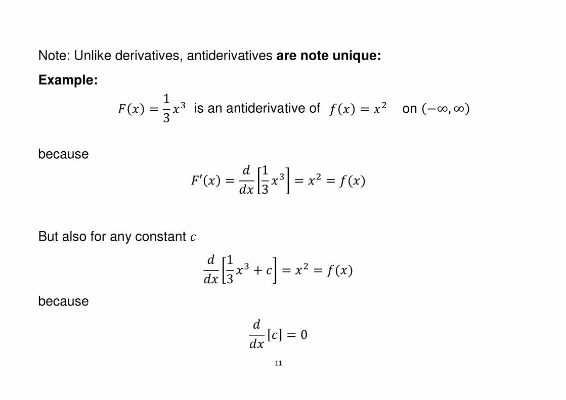
Note: Unlike derivatives, antiderivatives are note unique:
Example:
because
OU�� � ��� V13 �&W � �� � ���
But also for any constant � ��� V13 �& � �W � �� � ���
because ��� Q�S � 0
O�� � 13 �& is an antiderivative of ��� � �� on '∞, ∞�
12
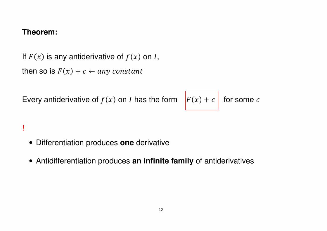
Theorem:
If O�� is any antiderivative of ��� on P,
then so is O�� � � Y "�� ����#"�#
Every antiderivative of ��� on P has the form O�� � � for some �
!
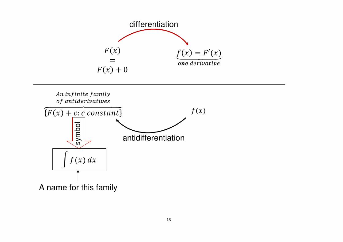
• Differentiation produces one derivative
• Antidifferentiation produces an infinite family of antiderivatives
13
O���O�� � 0 ��� � OU��Z[[[\[[[]^NF _`abcdebc`
differentiation
��� fO�� � �: � ����#"�#hijjjjjjkjjjjjjlmn bnobnbe` odpbq�ro dneb_`abcdebc`s
t ��� ��
A name for this family
antidifferentiation
sym
bo
l
14
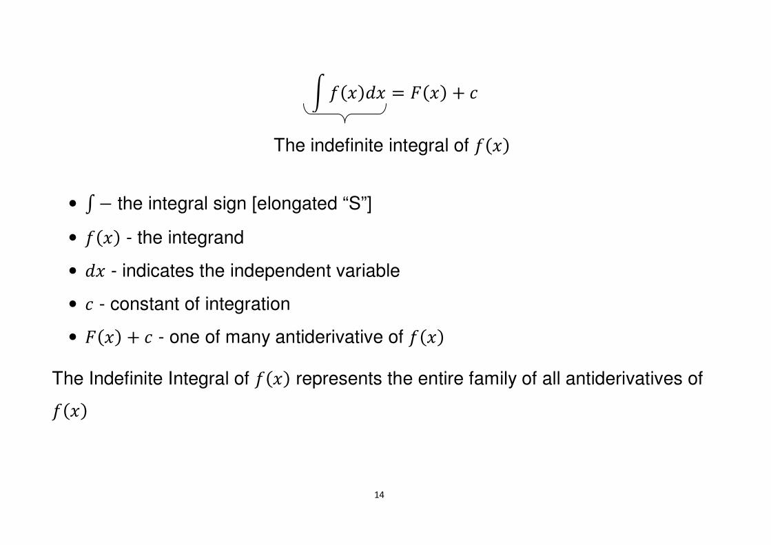
• u ' the integral sign [elongated “S”]
• ��� - the integrand
• �� - indicates the independent variable
• � - constant of integration
• O�� � � - one of many antiderivative of ���
The Indefinite Integral of ��� represents the entire family of all antiderivatives of
���
t ����� � O�� � �
The indefinite integral of ���
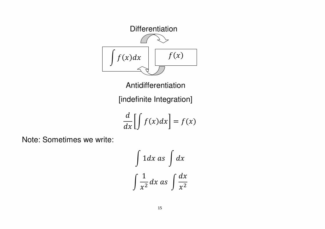
15
��� Vt �����W � ���
Note: Sometimes we write:
t 1�� "� t ��
t 1�� �� "� t ����
t ����� ���
Differentiation
Antidifferentiation
[indefinite Integration]
16
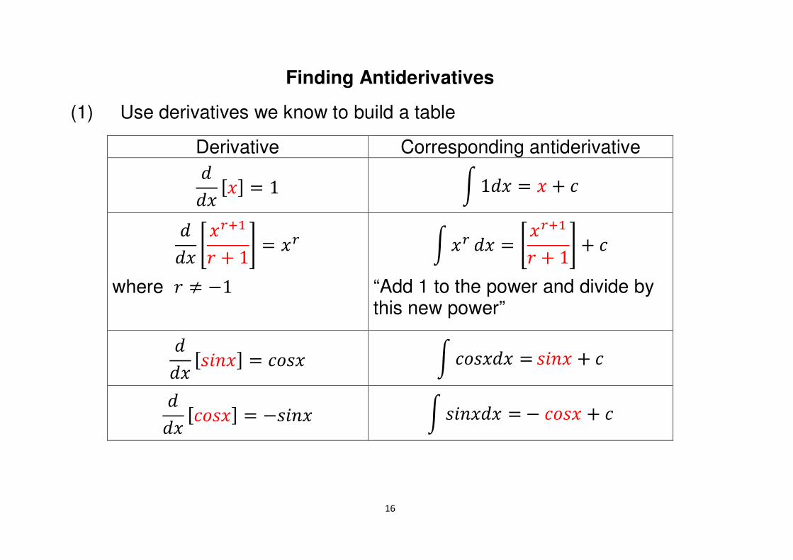
Finding Antiderivatives
(1) Use derivatives we know to build a table
Derivative Corresponding antiderivative ��� Q�S � 1 t 1�� � � � �
��� v �aw> � 1x � �a
where y '1
t �a �� � v �aw> � 1x � �
“Add 1 to the power and divide by this new power”
��� Q����S � ���� t ������ � ���� � �
��� Q����S � '���� t ������ � ' ���� � �
17
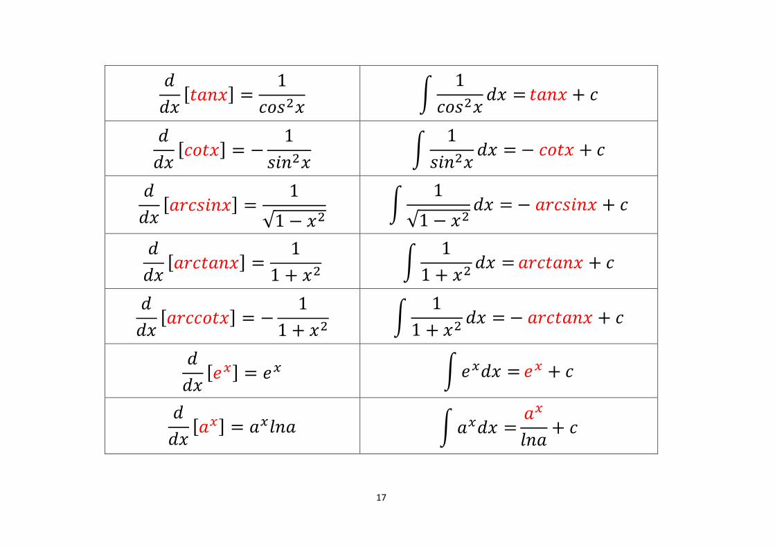
��� Q#"��S � 1����� t 1����� �� � #"�� � �
��� Q��#�S � ' 1����� t 1����� �� � ' ��#� � �
��� Q" �����S � 1√1 ' �� t 1√1 ' �� �� � ' " ����� � �
��� Q" �#"��S � 11 � �� t 11 � �� �� � " �#"�� � �
��� Q" ���#�S � ' 11 � �� t 11 � �� �� � ' " �#"�� � �
��� Q��S � �� t ���� � �� � �
��� Q"�S � "�$�" t "��� � "�$�" � �
18
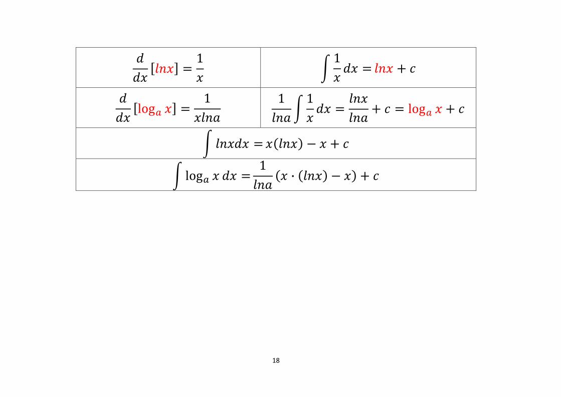
��� Q$��S � 1� t 1� �� � $�� � �
��� Qlogd �S � 1�$�" 1$�" t 1� �� � $��$�" � � � logd � � �
t $���� � �$��� ' � � �
t logd � �� � 1$�" � · $��� ' �� � �
19
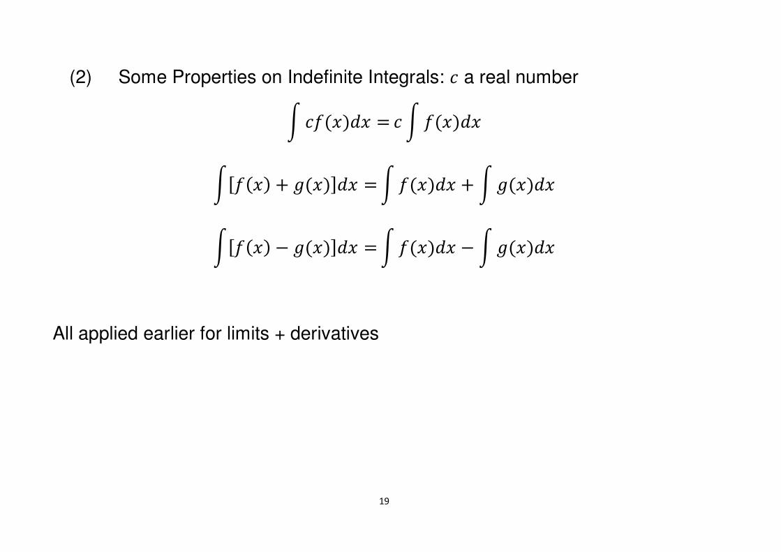
(2) Some Properties on Indefinite Integrals: � a real number
t ������ � � t �����
tQ��� � ~��S�� � t ����� � t ~����
tQ��� ' ~��S�� � t ����� ' t ~����
All applied earlier for limits + derivatives
20
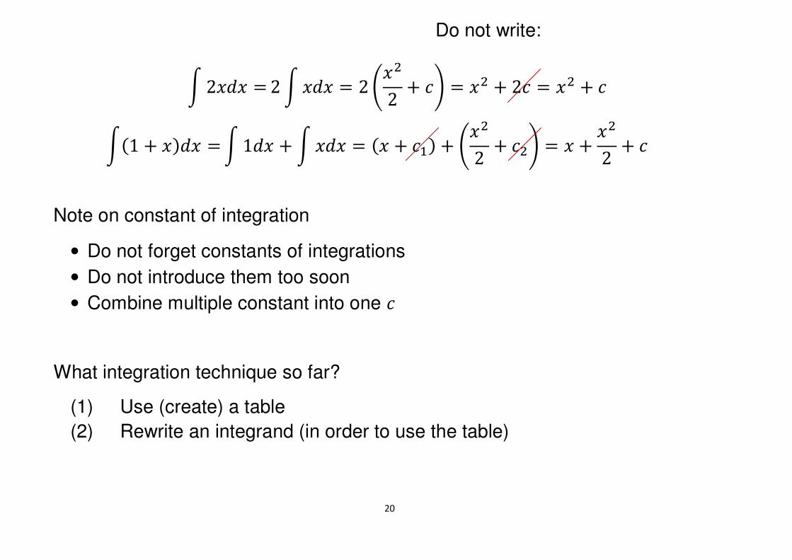
Note on constant of integration
• Do not forget constants of integrations
• Do not introduce them too soon
• Combine multiple constant into one �
What integration technique so far?
(1) Use (create) a table
(2) Rewrite an integrand (in order to use the table)
Do not write:
t 2��� � 2 t ��� � 2 6��2 � �7 � �� � 2� � �� � �
t1 � ���� � t 1�� � t ��� � � � �>� � 6��2 � ��7 � � � ��
2 � �
21
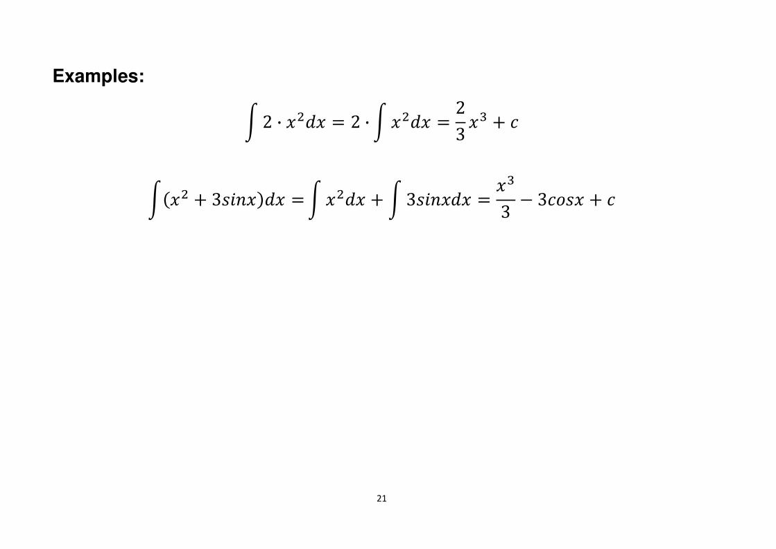
Examples:
t 2 · ���� � 2 · t ���� � 23 �& � �
t�� � 3������� � t ���� � t 3������ � �&3 ' 3���� � �
22
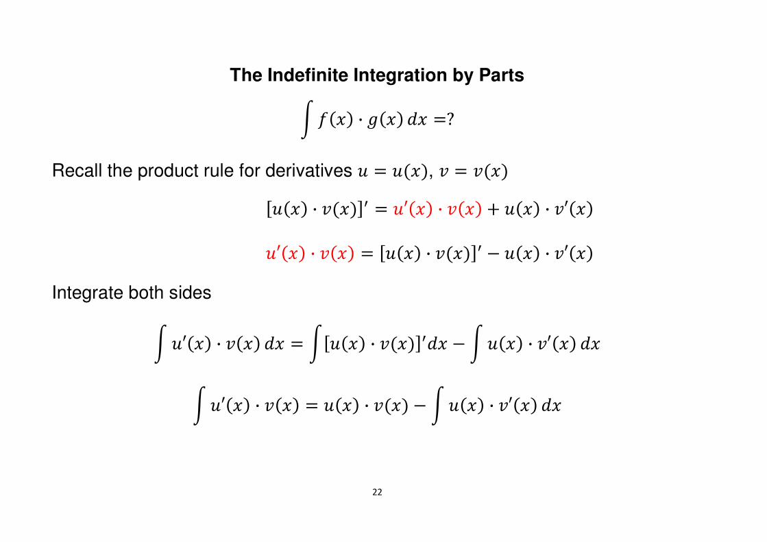
The Indefinite Integration by Parts
t ��� · ~�� �� �?
Recall the product rule for derivatives � � ���, % � %��
Integrate both sides
t �U�� · %�� �� � tQ��� · %��ST�� ' t ��� · %U�� ��
t �U�� · %�� � ��� · %�� ' t ��� · %U�� ��
Q��� · %��ST � �U�� · %�� � ��� · %U��
�U�� · %�� � Q��� · %��ST ' ��� · %U��
23
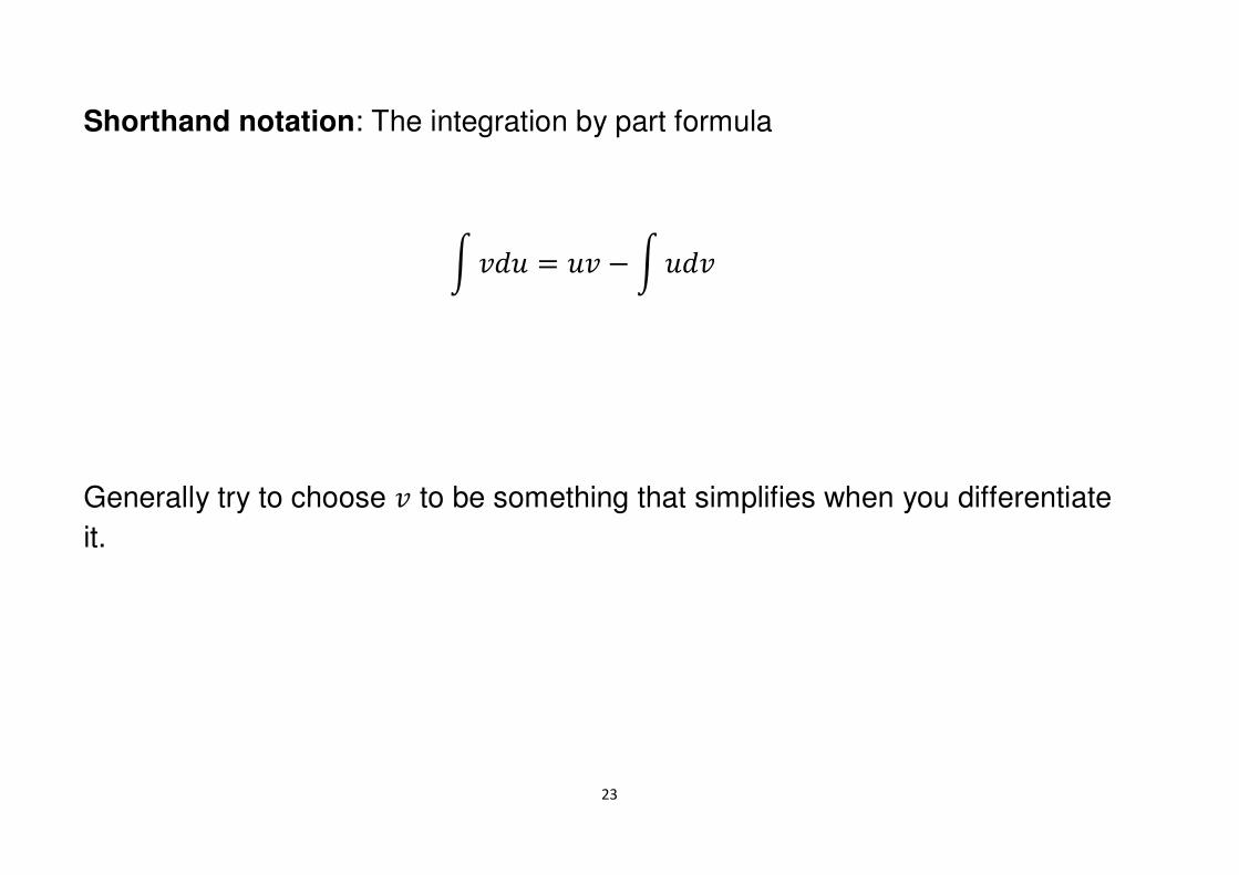
Shorthand notation: The integration by part formula
Generally try to choose % to be something that simplifies when you differentiate
it.
t %�� � �% ' t ��%
24
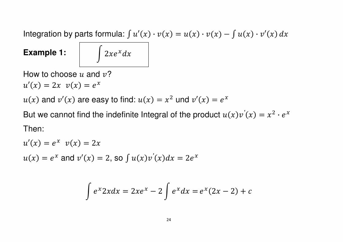
Integration by parts formula: u �U�� · %�� � ��� · %�� ' u ��� · %U�� ��
Example 1:
How to choose � and %? �U�� � 2� %�� � ��
��� and %U�� are easy to find: ��� � �� und %U�� � ��
But we cannot find the indefinite Integral of the product ���% ′�� � �� · ��
Then: �U�� � �� %�� � 2�
��� � �� and %U�� � 2, so u ���% ′���� � 2��
t ��2��� � 2��� ' 2 t ���� � ��2� ' 2� � �
t 2�����
25
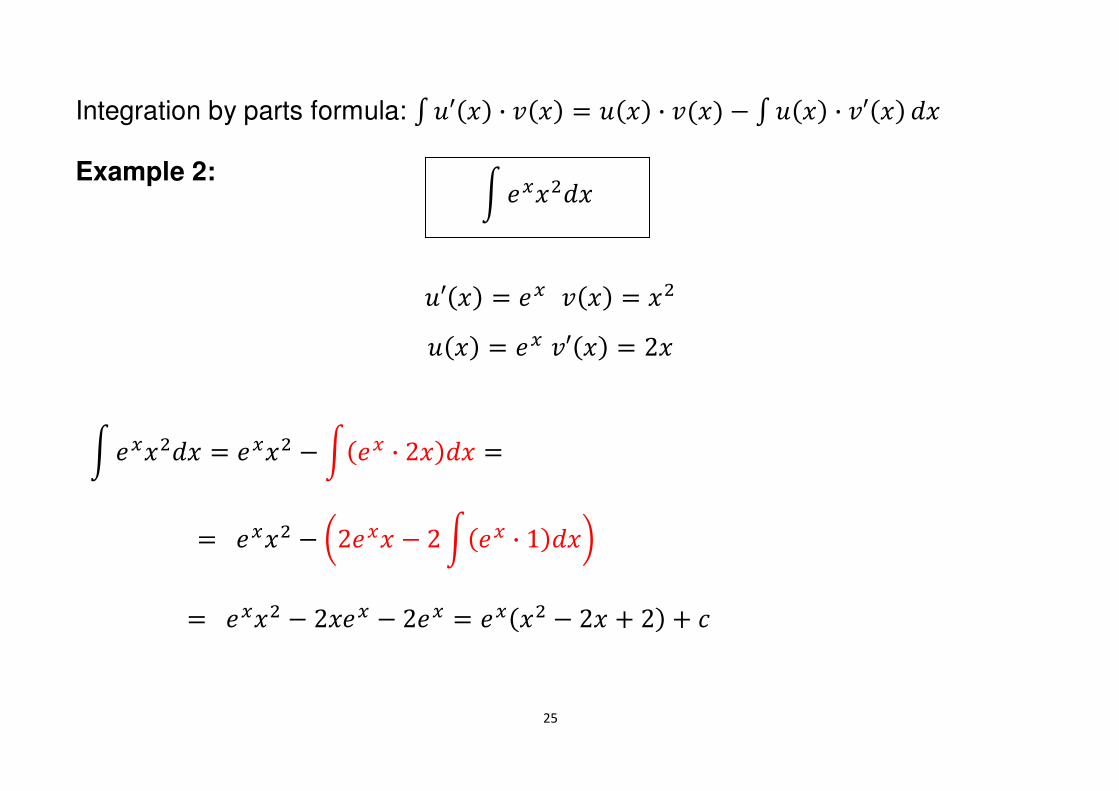
Integration by parts formula: u �U�� · %�� � ��� · %�� ' u ��� · %U�� ��
Example 2:
�U�� � �� %�� � ��
��� � �� %U�� � 2�
t ������
t ������ � ���� ' t�� · 2���� �
� ���� ' �2��� ' 2 t�� · 1����
� ���� ' 2��� ' 2�� � ���� ' 2� � 2� � �
26
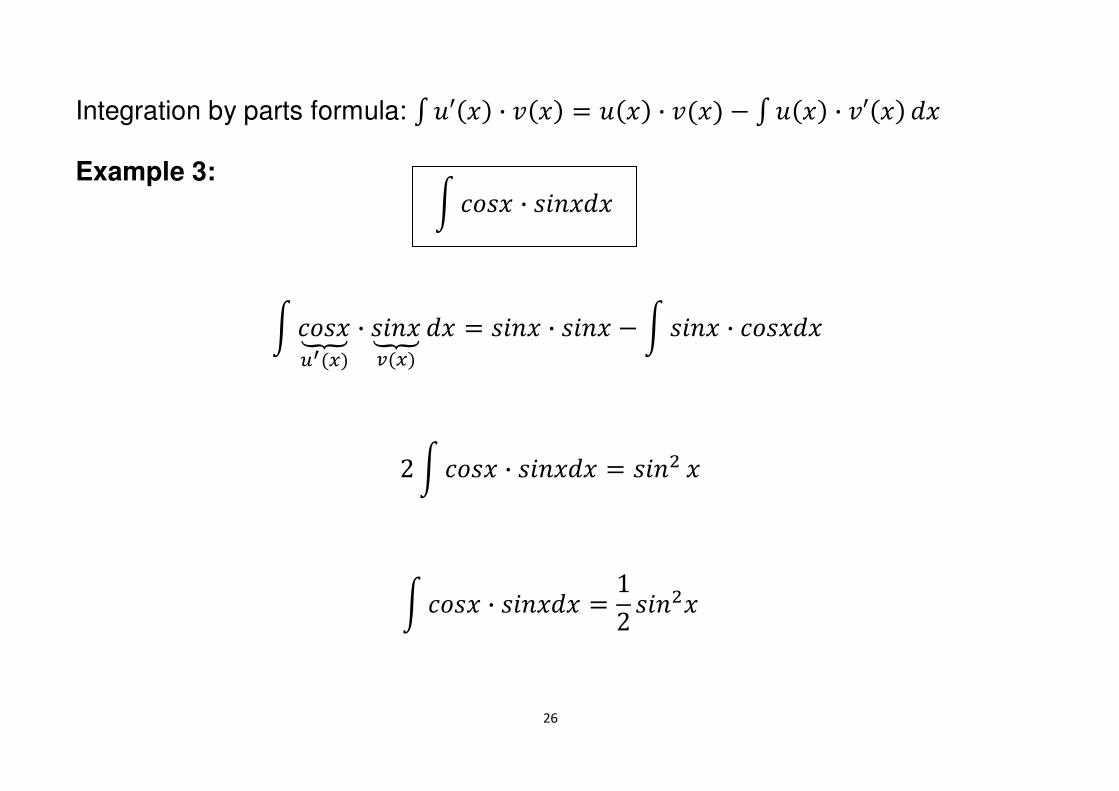
Integration by parts formula: u �U�� · %�� � ��� · %�� ' u ��� · %U�� ��
Example 3:
t ��������� · �����c�� �� � ���� · ���� ' t ���� · ������
2 t ���� · ������ � ���� �
t ���� · ������ � 12 �����
t ���� · ������

27
The Indefinite Integration by Substitution
Idea: Suppose OT � � and ~T exists
Chain rule: OU~��� � OT~���Z[[\[[]r�e`a · ~T��Z\]bnn`a
t OT�~��� · ~T�� �� � t OT�~���
So,
t �~��� · ~T�� �� � O~��� � �
Let � � ~��, then: ��~��� � K� ���� � ~T�� � ~T���� � DK
t ��� �� � O�� � �
Substitution of � for ~�� makes (when it works!) integration easier.
28
Straightforward Substitution
• Always consider “Substitution” first
• If on substitution fails, try another one!
Always make a total change from � to �! Never mix variables!
Substitution technique: Find something in the integrand to call � to simplifies the
appearance of the integral and whose �� � _�_� �� is also present as a factor
29
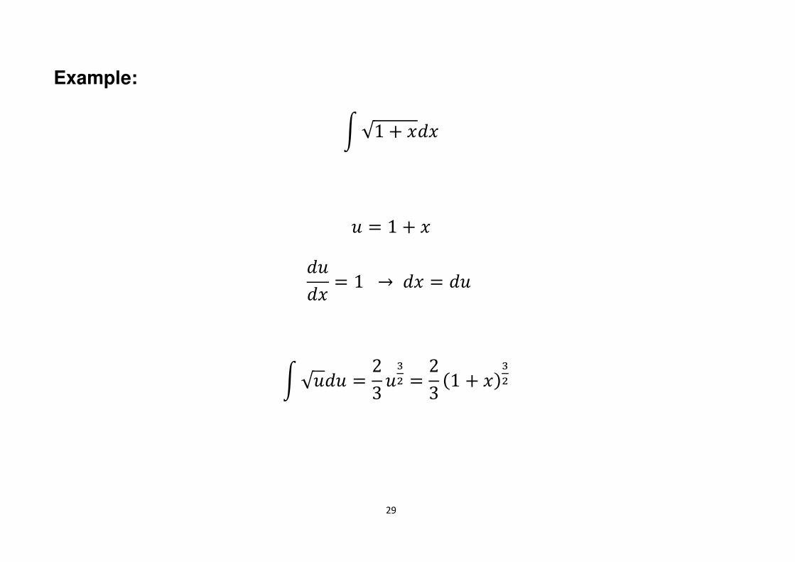
Example:
t √1 � ���
� � 1 � �
���� � 1 � �� � ��
t √��� � 23 ��� � 23 1 � ����
30
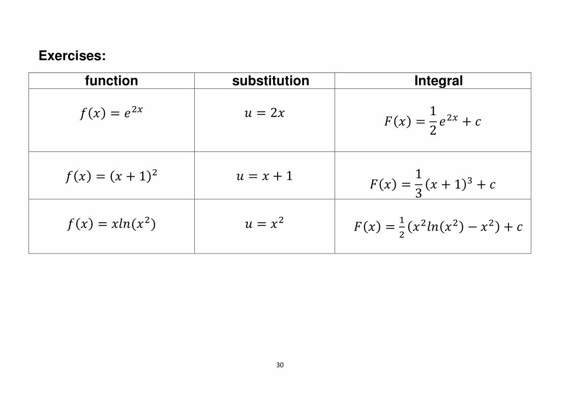
Exercises: function substitution Integral
��� � ���
� � 2�
O�� � 12 ��� � �
��� � � � 1��
� � � � 1
O�� � 13 � � 1�& � �
��� � �$����
� � ��
O�� � >� ��$���� ' ��� � �
31
Summary
A hard and fast set of rules for determining the method that should be used for
integration does not exist.
Some integrals can be done in more than one way.
It is possible that you will need to use more than one method to compute an
integral.
There are integrals that cannot be computed in terms of functions that we know.
32
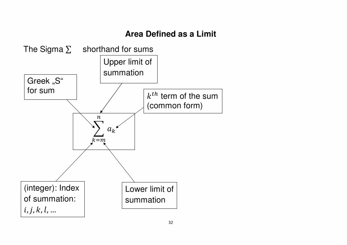
Area Defined as a Limit
The Sigma ∑ shorthand for sums
Upper limit of
summation
�e� term of the sum (common form)
Lower limit of
summation
Greek „S“ for sum
� "�n
��p
(integer): Index
of summation: �, �, �, $, …
33
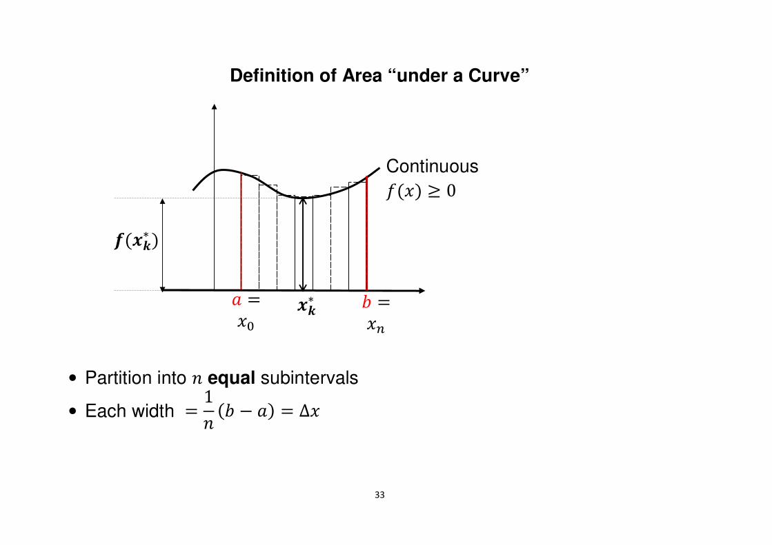
Definition of Area “under a Curve”
• Partition into � equal subintervals
• Each width
� 1� R ' "� � ∆�
" � �- ���
Continuous ��� � 0
R � �n
��� �
34
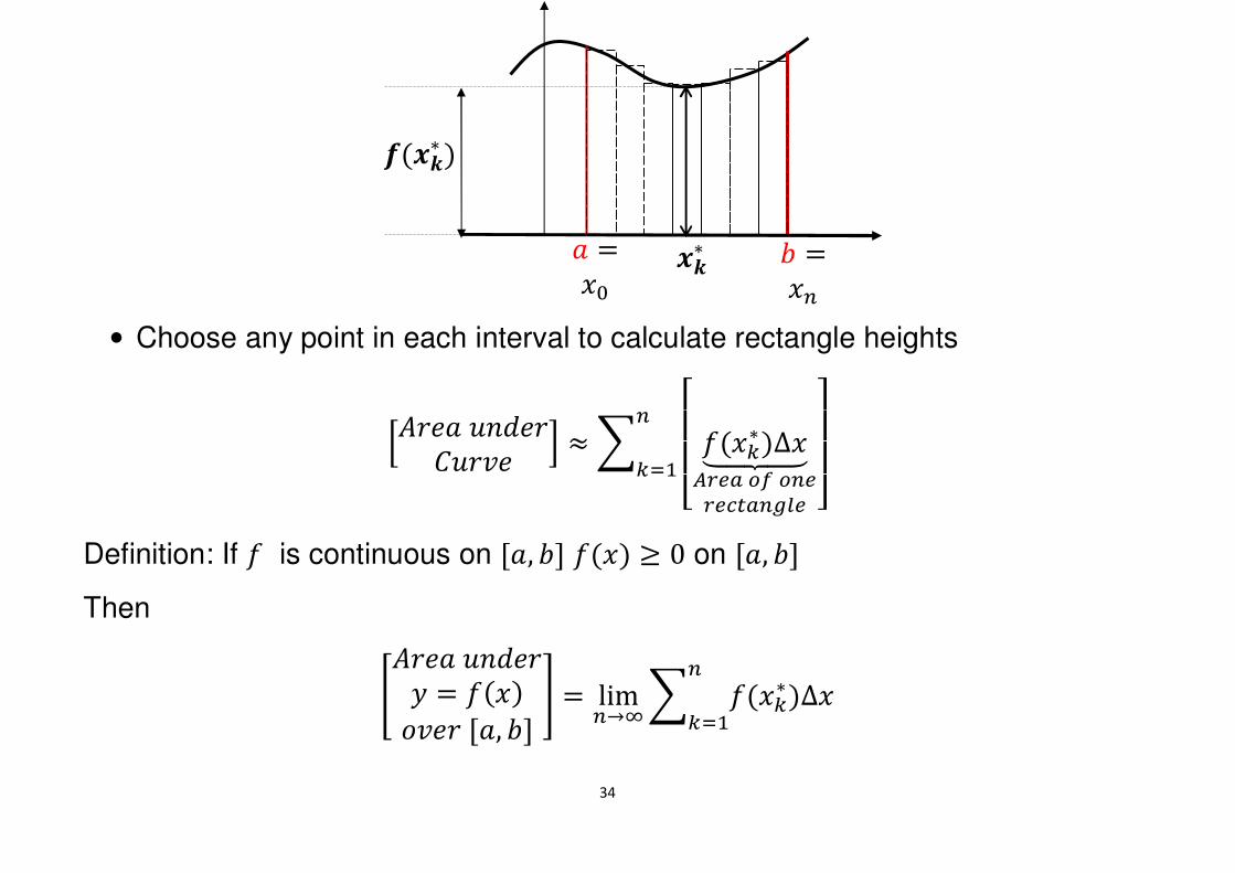
• Choose any point in each interval to calculate rectangle heights
�� �" ���� �� %� � � ����� �����∆�Z[\[]ma`d ro rn`a`�edn�q` �
¡n��>
Definition: If � is continuous on Q", RS ��� � 0 on Q", RS Then
¢� �" ���� � � ����%� Q", RS £ � limn�¦ � ����n��> �∆�
" � �- ��� R � �n
��� �
35
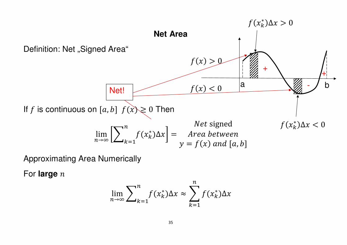
Net Area
Definition: Net „Signed Area“
If � is continuous on Q", RS ��� � 0 Then
limn�¦ V� ����n��> �∆�W � §�# signed� �" R�#¬���� � ��� "�� Q", RS
Approximating Area Numerically
For large � limn�¦ � ����n
��> �∆� � � �����∆�n��>
Net!
+
-
+
a b
�����∆� : 0
�����∆� ; 0
��� : 0
��� ; 0
36
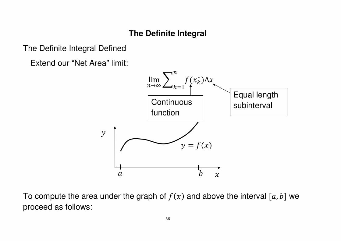
The Definite Integral
The Definite Integral Defined
Extend our “Net Area” limit:
To compute the area under the graph of ��� and above the interval Q", RS we
proceed as follows:
Continuous
function
Equal length
subinterval
" � R
� � � ���
limn�¦ � ����n��> �∆�
37
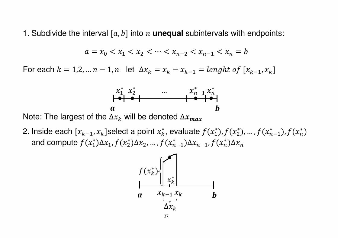
1. Subdivide the interval Q", RS into � unequal subintervals with endpoints:
" � �- ; �> ; �� ; ; �n®� ; �n®> ; �n � R
For each � � 1,2, … � ' 1, � let ∆�� � �� ' ��®> � $��~¯# �� Q��®>, ��S
Note: The largest of the ∆�� will be denoted ∆�IC�
2. Inside each Q��®>, ��Sselect a point ��� , evaluate ��>��, �����, … , ��n®>� �, ��n� �
and compute ��>��∆�>, �����∆��, … , ��n®>� �∆�n®>, ��n� �∆�n
C °
�>� ��� �n� �n®>�…
���
C ° ��®> ��
∆��
�����
38
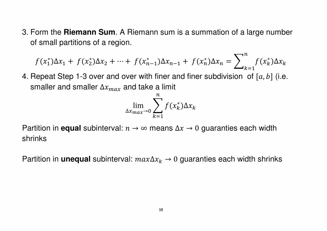
3. Form the Riemann Sum. A Riemann sum is a summation of a large number
of small partitions of a region.
��>��∆�> � �����∆�� � � ��n®>� �∆�n®> � ��n� �∆�n � � �����∆��n��>
4. Repeat Step 1-3 over and over with finer and finer subdivision of Q", RS (i.e.
smaller and smaller ∆�pd� and take a limit
lim∆�±²³�- � �����∆��n
��>
Partition in equal subinterval: � � ∞ means ∆� � 0 guaranties each width
shrinks
Partition in unequal subinterval: �"�∆�� � 0 guaranties each width shrinks
39
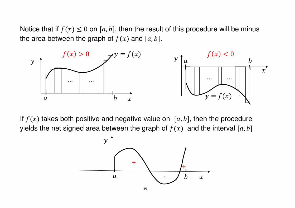
Notice that if ��� ´ 0 on Q", RS, then the result of this procedure will be minus
the area between the graph of ��� and Q", RS.
If ��� takes both positive and negative value on Q", RS, then the procedure
yields the net signed area between the graph of ��� and the interval Q", RS
+
-
+ " R �
�
"
�
R
�
� � ���
…
…
�
" � R
� � ���
… …
��� : 0 ��� ; 0
40
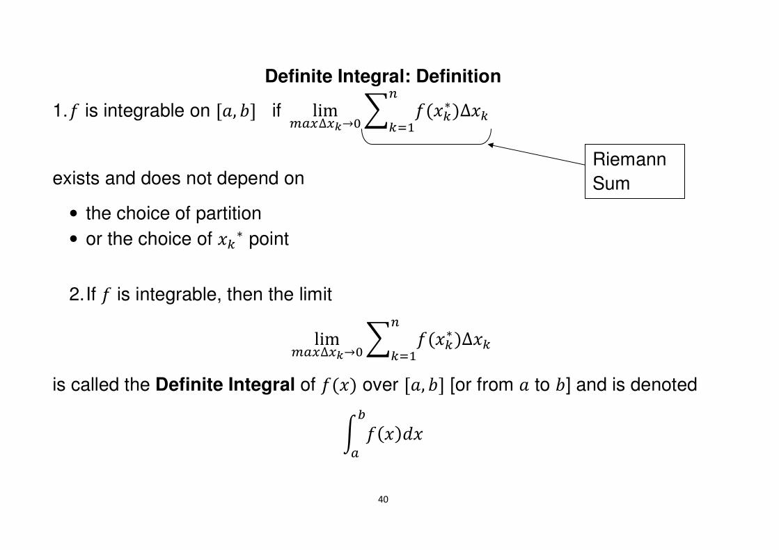
Definite Integral: Definition
1. � is integrable on Q", RS if
exists and does not depend on
• the choice of partition
• or the choice of ��� point
2. If � is integrable, then the limit
limpd�∆�µ�- � ����n��> �∆��
is called the Definite Integral of ��� over Q", RS [or from " to R] and is denoted
t �����¶d
limpd�∆�µ�- � ����n��> �∆��
Riemann
Sum
41
t �����¶d
": lower limit of integration
R: upper limit of integration
Be careful not to confuse u �����¶d and u �����. They are entirely different
types of things. The first is a number, the second is a collection of functions.
Notation:
∆� �
∆� � ��
∑ � u
42
The definite Integral of a continuous Function = Net “Area” under a curve
Theorem: If � is continuous on Q", RS then � is integrable on Q", RS And §�# · � �"R�#¬��� #¯�~ "!¯ �� �"�� Q", RS � t �����¶
d
Notation:
t Q��#�~ "��S����¶��d
43
We will need methods for evaluating the number
t �����¶d
other than computing the limit that defines them.
Some methods generally involve antidifferentiation, but some definite integrals
can be evaluated by thinking of them as area.
44
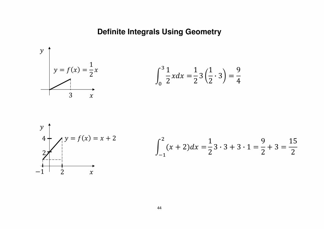
Definite Integrals Using Geometry
� � ��� � � � 2
�
�
2 '1
2
4
�
�
3
� � ��� � 12 � t 12 ��� �&-
12 3 �12 · 3� � 94
t � � 2��� ��®>
12 3 · 3 � 3 · 1 � 92 � 3 � 152
45
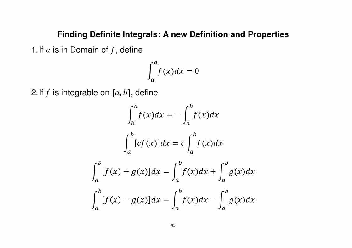
Finding Definite Integrals: A new Definition and Properties
1. If " is in Domain of �, define
t �����dd � 0
2. If � is integrable on Q", RS, define
t �����d¶ � ' t �����¶
d
t Q����S��¶d � � t �����¶
d
t Q��� � ~��S��¶d � t �����¶
d � t ~����¶d
t Q��� ' ~��S��¶d � t �����¶
d ' t ~����¶d
46
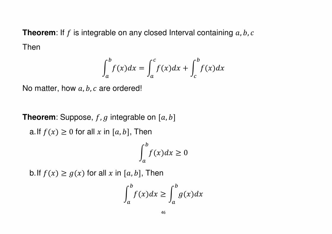
Theorem: If � is integrable on any closed Interval containing ", R, �
Then
t �����¶d � t ������
d � t �����¶�
No matter, how ", R, � are ordered!
Theorem: Suppose, �, ~ integrable on Q", RS a. If ��� � 0 for all � in Q", RS, Then
t �����¶d � 0
b. If ��� � ~�� for all � in Q", RS, Then
t �����¶d � t ~����¶
d
47
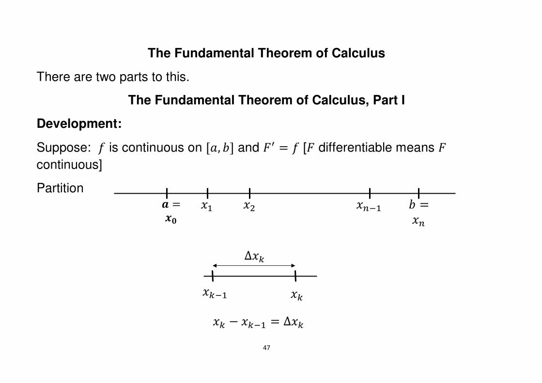
The Fundamental Theorem of Calculus
There are two parts to this.
The Fundamental Theorem of Calculus, Part I
Development:
Suppose: � is continuous on Q", RS and OT � � [O differentiable means O
continuous]
Partition C � �H
R � �n
�> �� �n®>
��®> ��
�� ' ��®> � ∆��
∆��
48
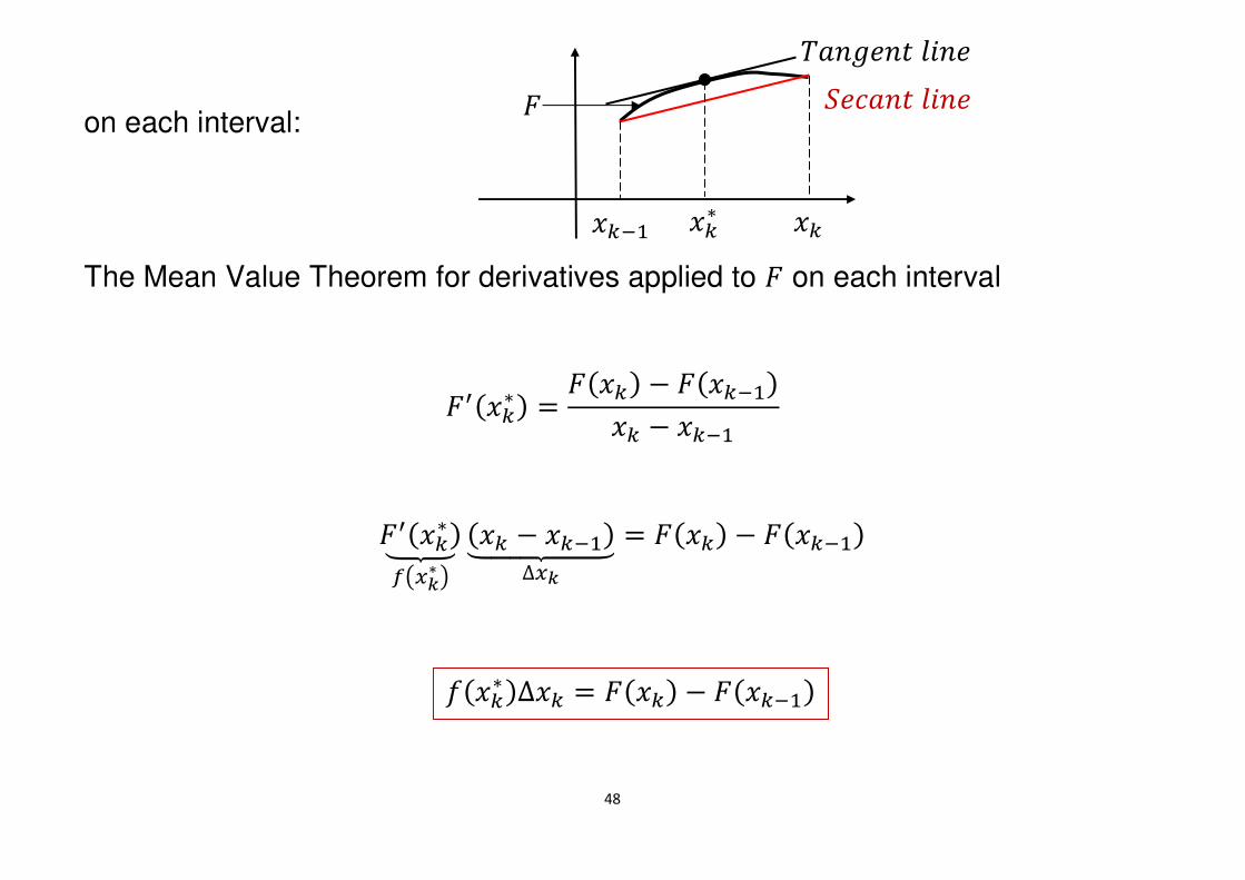
on each interval:
The Mean Value Theorem for derivatives applied to O on each interval
OT���� � O��� ' O��®>��� ' ��®>
OT����Z\]o��µ� ��� ' ��®>�Z[[[\[[[]∆�µ
� O��� ' O��®>�
��®> �� ���
O º��"�# $���
»"�~��# $���
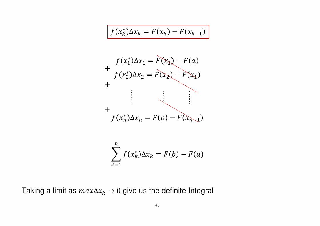
���� �∆�� � O��� ' O��®>�
49
��>��∆�> � O�>� ' O"�
�����∆�� � O��� ' O�>�
��n� �∆�n � OR� ' O�n®>�
� �����∆��n
��>� OR� ' O"�
Taking a limit as �"�∆�� � 0 give us the definite Integral
���� �∆�� � O��� ' O��®>�
�
�
�
50
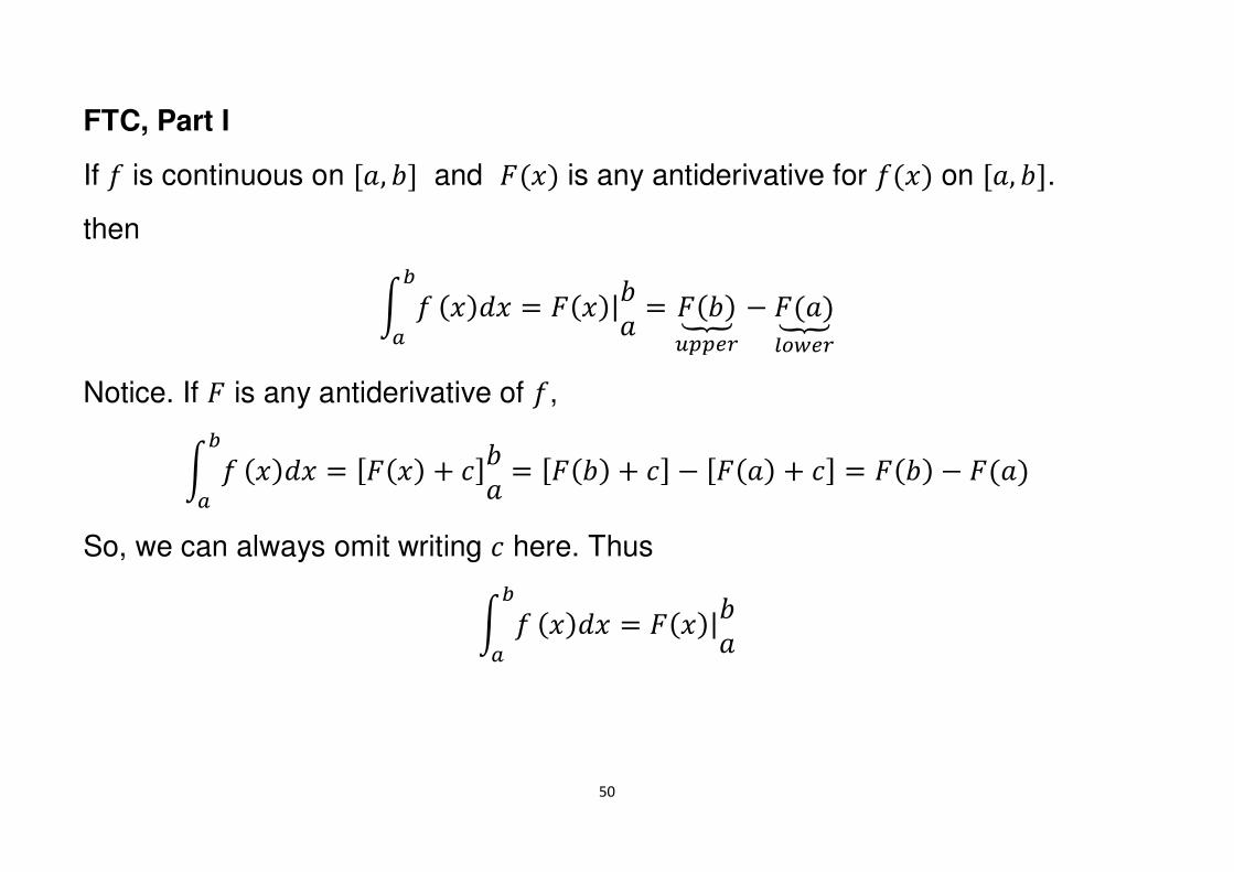
FTC, Part I
If � is continuous on Q", RS and O�� is any antiderivative for ��� on Q", RS. then
t �¶d ���� � �O��|R" � OR���½½`a ' O"��qr¾`a
Notice. If O is any antiderivative of �,
t �¶d ���� � QO�� � �SR" � QOR� � �S ' QO"� � �S � OR� ' O"�
So, we can always omit writing � here. Thus
t �¶d ���� � �O��|R"
51
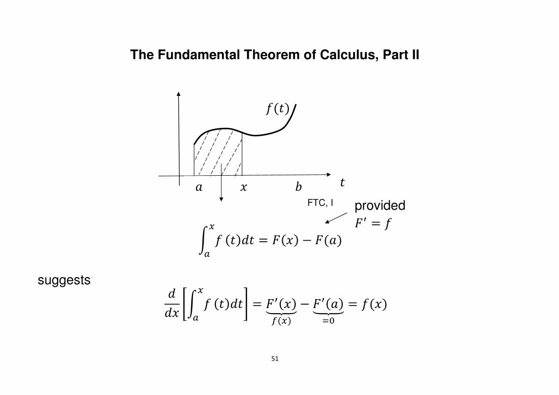
The Fundamental Theorem of Calculus, Part II
t ��d #��# � O�� ' O"�
providedOT � �
FTC, I
# " R
�#�
�
��� vt ��d #��#x � OT��Z\]o�� ' OT"�Z\]�- � ���
suggests
52
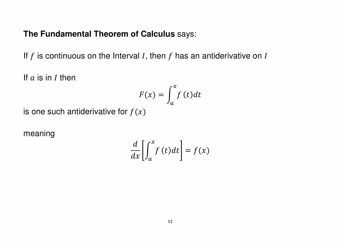
The Fundamental Theorem of Calculus says:
If � is continuous on the Interval P, then � has an antiderivative on P
If " is in P then
O�� � t ��d #��#
is one such antiderivative for ���
meaning ��� vt ��d #��#x � ���
53
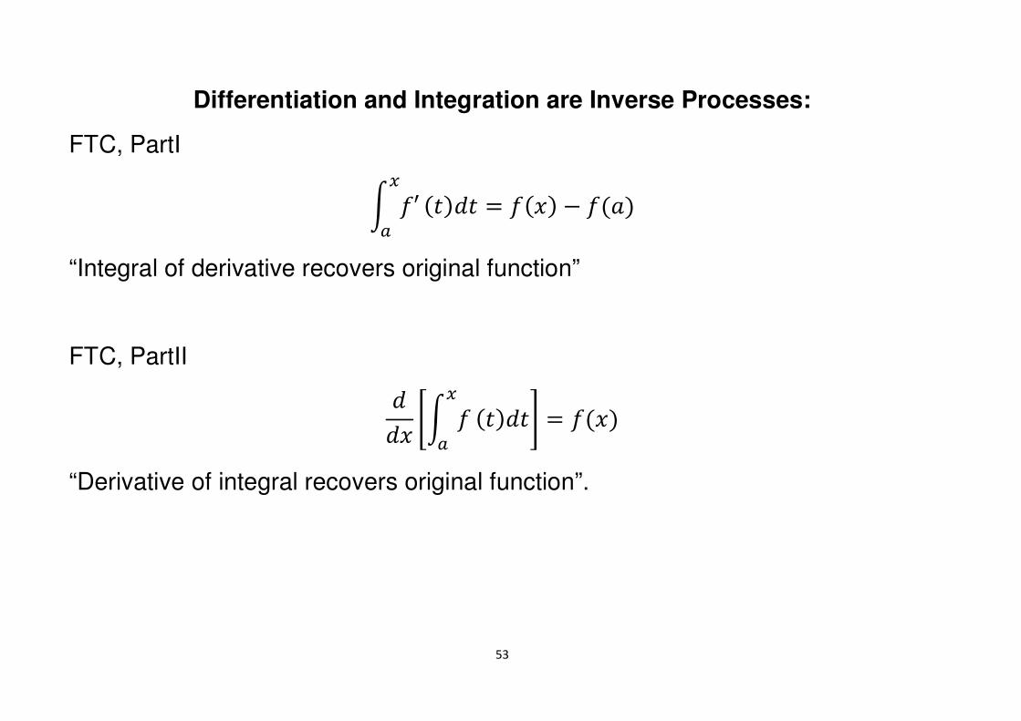
Differentiation and Integration are Inverse Processes:
FTC, PartI
t �U�d #��# � ��� ' �"�
“Integral of derivative recovers original function”
FTC, PartII
��� vt ��d #��#x � ���
“Derivative of integral recovers original function”.
54
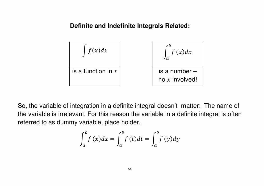
Definite and Indefinite Integrals Related:
So, the variable of integration in a definite integral doesn’t matter: The name of
the variable is irrelevant. For this reason the variable in a definite integral is often
referred to as dummy variable, place holder.
t �¶d ���� � t �¶
d #��# � t �¶d ����
t �����
t �¶d ����
is a function in �
is a number –
no � involved!
55
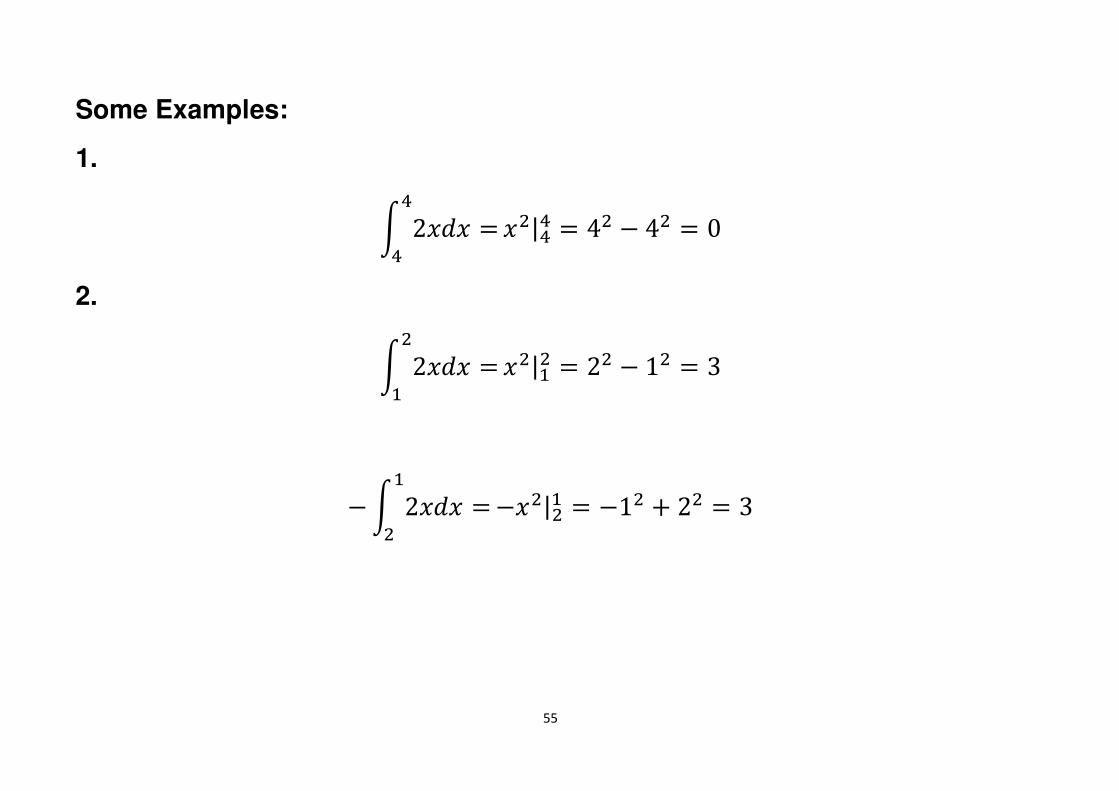
Some Examples:
1.
t 2��� �?? ���|?? � 4� ' 4� � 0
2.
t 2��� ��> ���|>� � 2� ' 1� � 3
' t 2��� �>� �'��|�> � '1� � 2� � 3
56
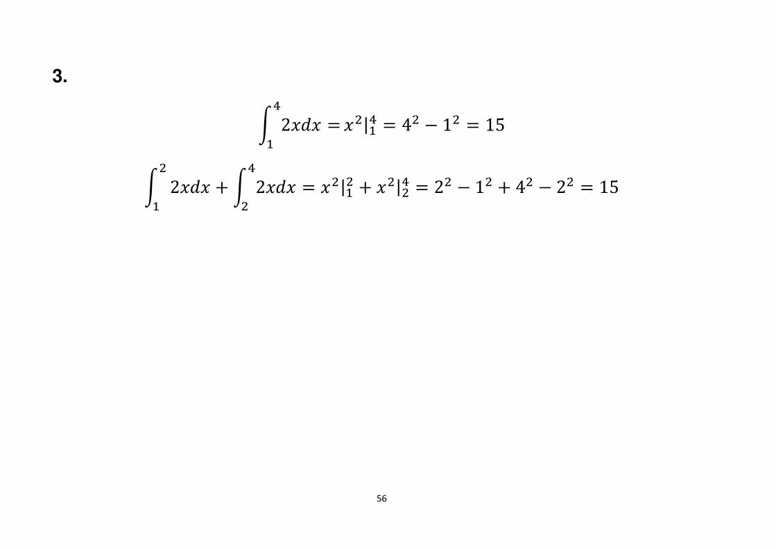
3.
t 2��� �?> ���|>? � 4� ' 1� � 15
t 2��� � t 2��� � ���|>�?
��
> � ���|�? � 2� ' 1� � 4� ' 2� � 15
57
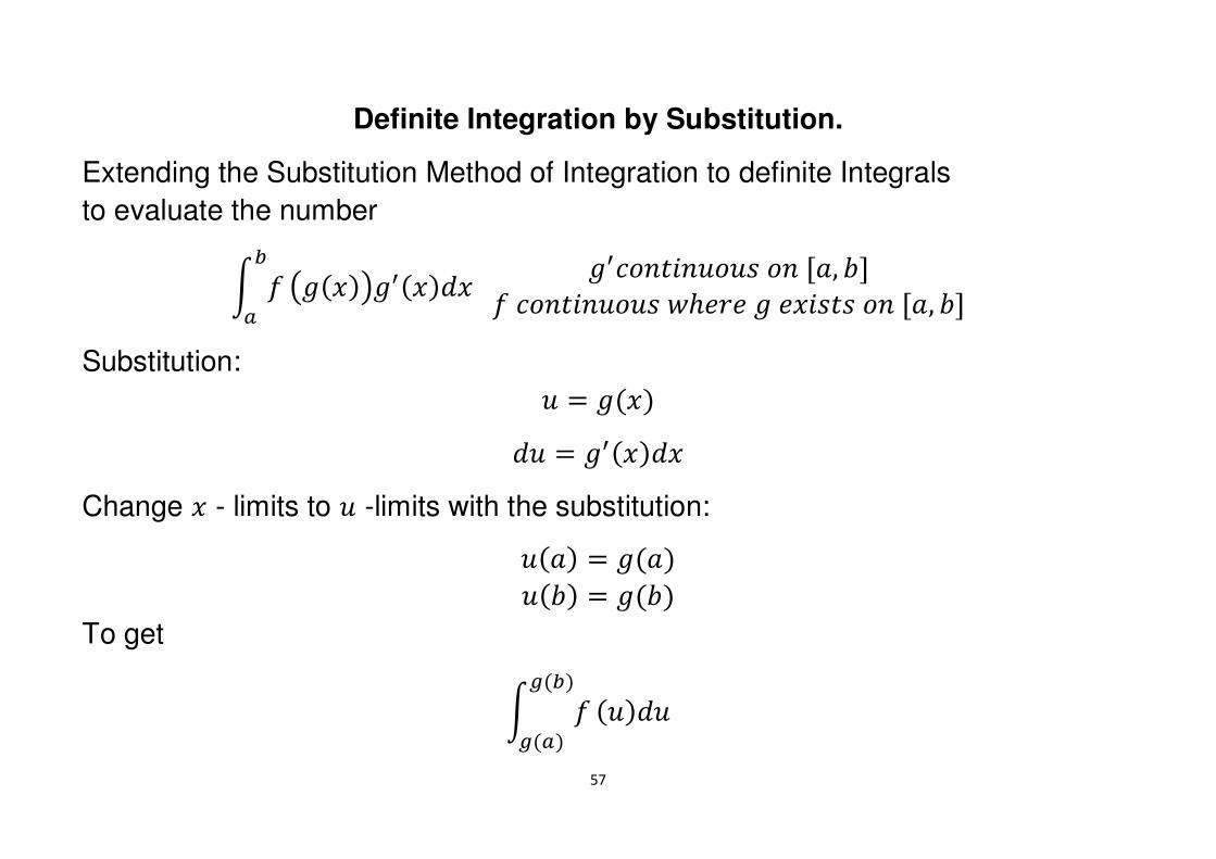
Definite Integration by Substitution.
Extending the Substitution Method of Integration to definite Integrals
to evaluate the number
t �¶d �~���~T���� ~T���#������ �� Q", RS� ���#������ ¬¯� � ~ ����#� �� Q", RS
Substitution: � � ~��
�� � ~T����
Change � - limits to � -limits with the substitution:
�"� � ~"��R� � ~R�
To get
t ��¶��d� ����
58
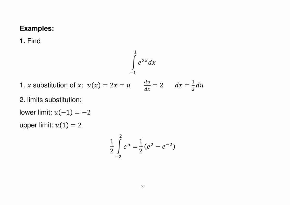
Examples:
1. Find
t �����>®>
1. � substitution of �: ��� � 2� � � _�_� � 2 �� � >� ��
2. limits substitution:
lower limit: �'1� � '2
upper limit: �1� � 2
12 t �� ��®�
12 �� ' �®��
59
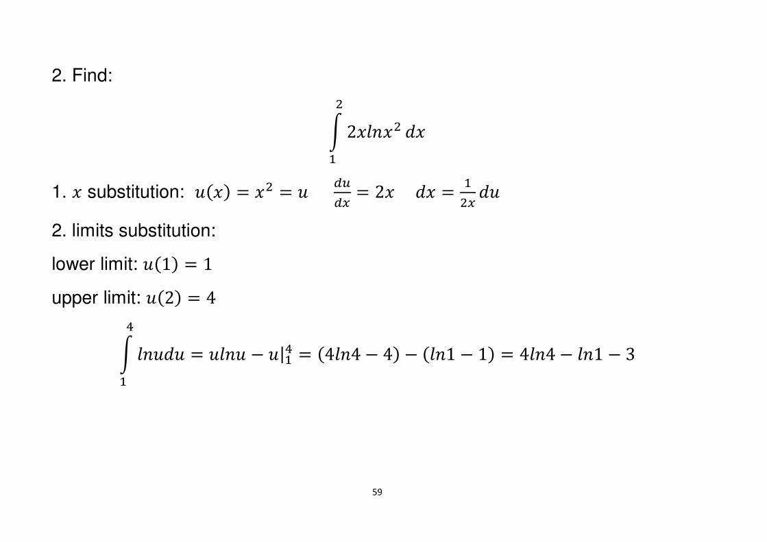
2. Find:
t 2�$����>
��
1. � substitution: ��� � �� � � _�_� � 2� �� � >�� ��
2. limits substitution:
lower limit: �1� � 1
upper limit: �2� � 4
t $���� � ��$�� ' �|>??
>� 4$�4 ' 4� ' $�1 ' 1� � 4$�4 ' $�1 ' 3
60
The Definite Integral Applied
Total Area
Although
t �¶d ���� ' "��# " �""
We can find that
� #�#"$� �" � � t |���|¶d ��
61
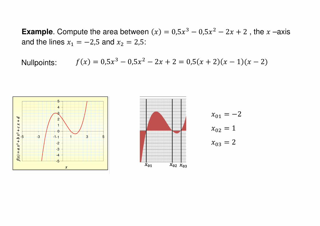
Example. Compute the area between �� � 0,5�& ' 0,5�� ' 2� � 2 , the � –axis
and the lines �> � '2,5 and �� � 2,5:
-5
-4
-3
-2
-1
0
1
2
3
4
5
-5 -3 -1 1 3 5
f(x)
= a
x³
+ b
x²
+ c
x +
d
x
-5
-4
-3
-2
-1
0
1
2
3
4
5
�HG �HA �H@
�-> � '2
�-� � 1
�-& � 2
Nullpoints: ��� � 0,5�& ' 0,5�� ' 2� � 2 � 0,5� � 2�� ' 1�� ' 2�
62
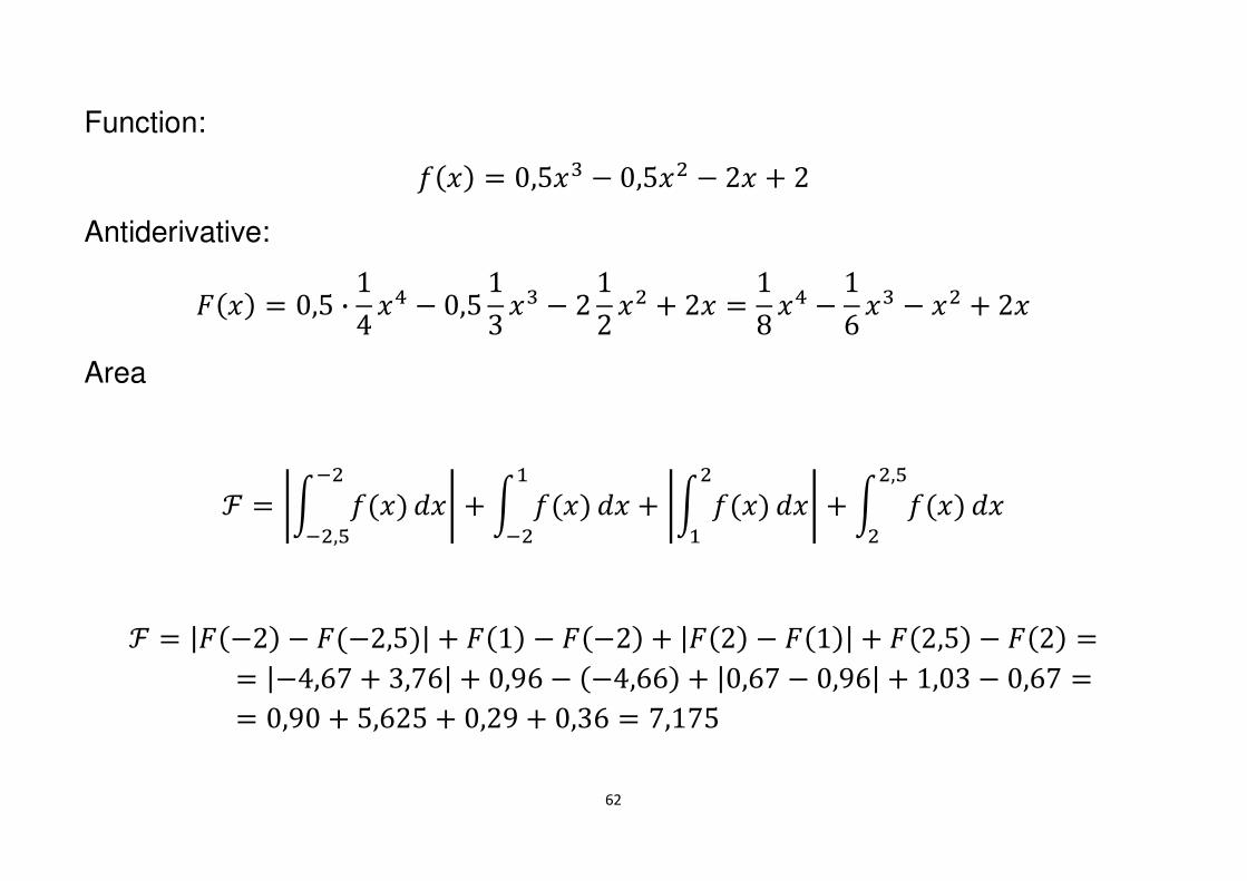
Function:
��� � 0,5�& ' 0,5�� ' 2� � 2
Antiderivative:
O�� � 0,5 · 14 �? ' 0,5 13 �& ' 2 12 �� � 2� � 18 �? ' 16 �& ' �� � 2�
Area
Á � Ât ���®�®�,à �� � t ���>
®� �� � Ât ����> �� � t ����,Ã
� ��
Á � |O'2� ' O'2,5�| � O1� ' O'2� � |O2� ' O1�| � O2,5� ' O2� �� |'4,67 � 3,76| � 0,96 ' '4,66� � |0,67 ' 0,96| � 1,03 ' 0,67 �� 0,90 � 5,625 � 0,29 � 0,36 � 7,175
63
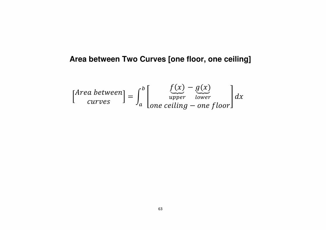
Area between Two Curves [one floor, one ceiling]
�� �" R�#¬����� %�� � � t ¢ �����½½`a ' ~���qr¾`a��� ���$��~ ' ��� �$�� £¶d ��
64
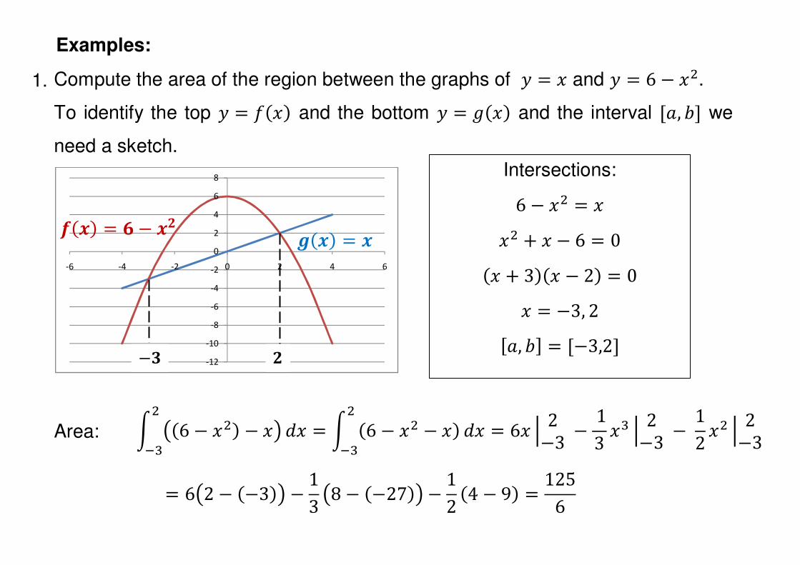
Compute the area of the region between the graphs of � � � and � � 6 ' ��.
To identify the top � � ��� and the bottom � � ~�� and the interval Q", RS we
need a sketch.
Area:
-12
-10
-8
-6
-4
-2
0
2
4
6
8
-6 -4 -2 0 2 4 6
�� � � �� � Š' �G
'A G
6 ' �� � �
�� � � ' 6 � 0
� � 3�� ' 2� � 0
� � '3, 2
Q", RS � Q'3,2S
Intersections:
t �6 ' ��� ' ���®& �� � t 6 ' �� ' ���
®& �� � 6� Æ 2'3 � ' 13 �& Æ 2'3 � ' 12 �� Æ 2'3�
� 6�2 ' '3�� ' 13 �8 ' '27�� ' 12 4 ' 9� � 1256
Examples:
1.
65
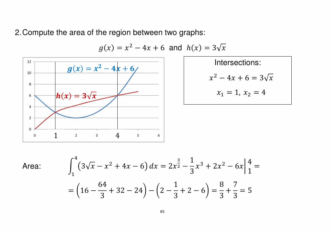
Compute the area of the region between two graphs:
~�� � �� ' 4� � 6 and ¯�� � 3√�
Area:
0
2
4
6
8
10
12
0 1 2 3 4 5 6
Ç�� � A√�
Ä�� � �G ' L� � Å
1 4
�� ' 4� � 6 � 3√�
�> � 1, �� � 4
Intersections:
� �16 ' 643 � 32 ' 24� ' �2 ' 13 � 2 ' 6� � 83 � 73 � 5
t �3√� ' �� � 4� ' 6�?> �� � �2��� ' 13 �& � 2�� ' 6�È 41 �
2.