The Lognormal Distribution

By: Brian Shaw and Tim David

What is a Lognormal?

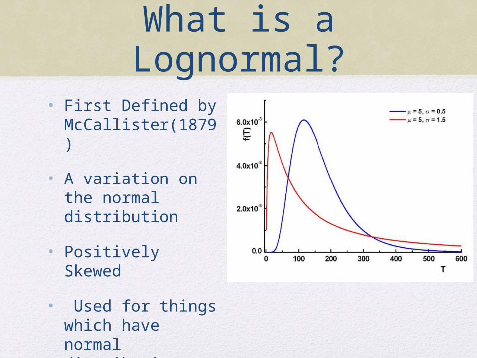
• First Defined by McCallister(1879)

• A variation on the normal distribution

• Positively Skewed

• Used for things which have normal distributions with only positive values

Derivation of Lognormal

• A distribution whose logarithm is normally distributed

• Let Y=lnX=v(y)

• v’(y)=1/x

• g(y)=[f(v(y))][v’(y)]

• Similar to normal is defined for all positive values: 0≤x≤∞

Normal:

Lognormal:€

12πσ

e−(x−μ )2

2σ 2

€

1x 2πσ

e−(ln(x )−μ )2

2σ 2

Some Properties of Lognormal

• C.D.F.• We could Integrate

• That’s Hard • Make it Standard

Normal

€

φ ln x −μσ

⎛ ⎝ ⎜

⎞ ⎠ ⎟€

12πσ

1te

−(ln( t )−μ )2

2σ 2

0

x

∫ dt

Some Properties of Lognormal

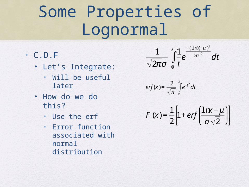
• C.D.F• Let’s Integrate:

• Will be useful later

• How do we do this?• Use the erf• Error function

associated with normal distribution

€

12πσ

1te

−(ln( t )−μ )2

2σ 2

0

x

∫ dt

€

F(x) = 12

1+ erf ln x −μσ 2

⎛ ⎝ ⎜

⎞ ⎠ ⎟

⎡ ⎣ ⎢

⎤ ⎦ ⎥€

erf (x) =2π

e−t 2

dt0

x

∫

Some Properties of Lognormal

• Normalization:• For computational

simplicity we let y=ln(x) and differentiate

• Then: dy=dx/x• Also realize that ey=x• This allows to write

the lognormal as a normal distribution

€

12πσ

1xe

−(ln(x )−μ )2

2σ 2

0

∞

∫ dx =1

€

12πσ

e−(y−μ )2

2σ 2

−∞

∞

∫ dy =1

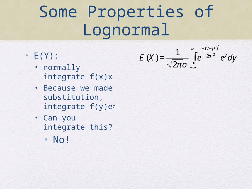
Some Properties of Lognormal

• E(Y): • normally integrate

f(x)x • Because we made

substitution, integrate f(y)ey

• Can you integrate this?• No!

€

E(X) = 12πσ

e−(y−μ )2

2σ 2

−∞

∞

∫ eydy

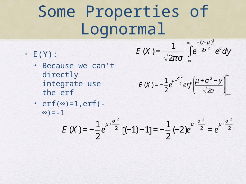
Some Properties of Lognormal

• E(Y):• Because we can’t

directly integrate use the erf

• erf(∞)=1,erf(-∞)=-1

€

E(X) = 12πσ

e−(y−μ )2

2σ 2

−∞

∞

∫ eydy

€

E(X) = − 12eμ +σ 2

2 erf μ +σ 2 − y2σ

⎛ ⎝ ⎜

⎞ ⎠ ⎟−∞

∞

€

E(X) = − 12eμ +σ 2

2 (−1) −1[ ] = − 12

(−2)eμ +σ 2

2 = eμ +σ 2

2

Some Properties of Lognormal

• Var(X)• Similarly we can

computer the variance of a lognormal

€

Var (X) = E(X 2) −μ 2

= 12πσ

e−(y−μ )2

2σ 2

−∞

∞

∫ e2ydy − eμ +σ 2

2 ⎛

⎝ ⎜ ⎜

⎞

⎠ ⎟ ⎟

2

= eσ2 +2μ (eσ

2

−1)

Skewness: A Defining Characteristic

• The major difference between lognormal and normal distribution• Positive Domain• Positive Skewness

Skewness: A Defining Characteristic

• What is skewness?• A measure of asymmetry in a

distribution• Defined by a Ratio:• Positive Ratio:

• Long R.H. Tail• Negative ratio:

• Long L.H. Tail• Ratio=0

• Symetric

€

γ1 = μ3

μ23 / 2

Skewness: A Defining Characteristic

• For a lognormal distribution, skewness is defined by the formula:

€

eσ2

−1 2 + eσ2

( )

Mode: An old friend with a new take

• Because the Lognormal distribution is skewed, the mean is not at the peak• This makes sense,

because the tails are uneven.

Mode: An old friend with a new take

• Because of this problem we use the mode to describe the peak.• We can find the

mode by maximizing the p.d.f• Do this by taking

the derivative and setting it to zero

€

f (x) = 1x 2πσ

e−(ln(x )−μ )2

2σ 2

€

f '(x) = 0

€

Mode(X ) = eμ−σ 2

Putting It All Together

• Lets take a look at the first graph we had and apply some of things we learned.

• Two Curves:• μ=5, σ2=.25(Blue)• Μ=5,

σ2=2.25(Red)

Putting It All Together

• Properties A Curve:• Blue

• Mean: 168• Variance: 8033• Mode: 115• Skewness:1.75

• Red• Mean:457• Variance: 1773777• Mode: 15• Skewness: 33

Mode

Mean

Which of these is not Lognormally Distributed?

• Number of crystals in Ice Cream• Survival time after diagnosis in cancer• Age of marriage of women (Denmark)• Air pollution in PSI (Los Angeles)• Length of spoken words in phone conversation• Farm size in Wales(1989)• The height of St. Mary’s Students

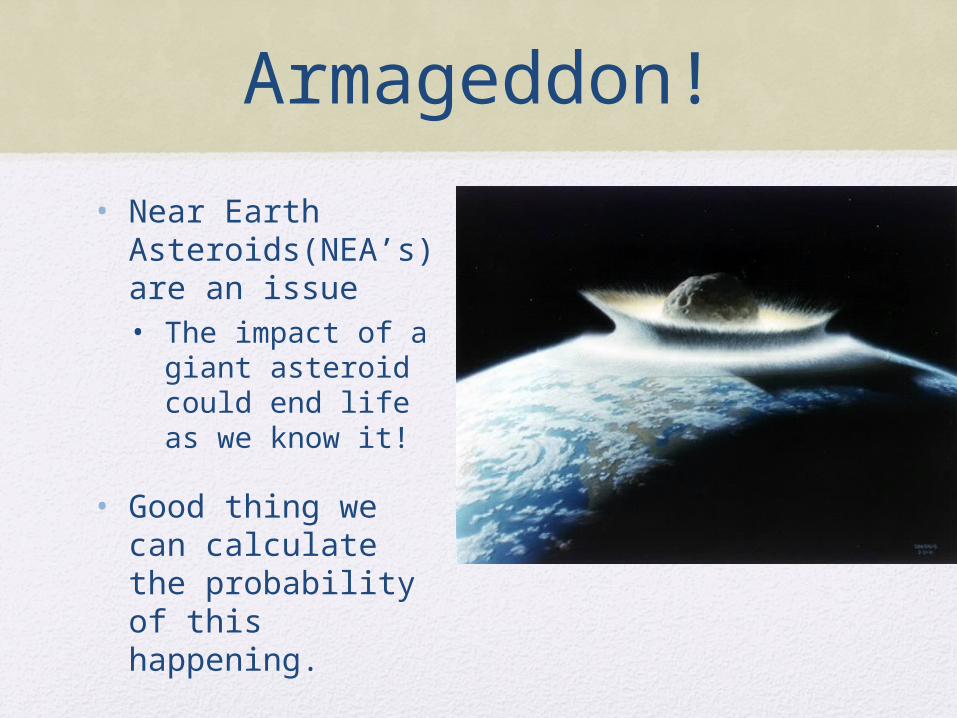
Armageddon!• Near Earth

Asteroids(NEA’s) are an issue• The impact of a

giant asteroid could end life as we know it!

• Good thing we can calculate the probability of this happening.

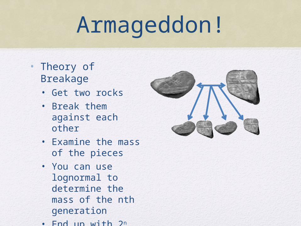
Armageddon!• Theory of Breakage

• Get two rocks• Break them

against each other• Examine the mass

of the pieces• You can use

lognormal to determine the mass of the nth generation

• End up with 2n rocks

Armageddon!• As you can see, this would also apply to

asteroids.• They are just big rocks.

• Traditionally, used the power law to describe the size of asteroids• Limitation: Couldn’t take single events

into accounts. Theory of breakage allows us to do this

• Therefore, we can use the lognormal!

Armageddon! (With Math)

• NEA’s come from fragmentation in the Main Asteroid Belt

• From the data we have, we can model how many NEA’s are large enough to cause a significant problem.• This is because the crater is

proportional to the asteroid size.

Armageddon! (With Math)

• Recently, estimations of NEA’s have shown that there are less significantly large NEA’s than once thought

• This is supported by the math:• If we classify the asteroid size into two

lognormal distributions, we get similar results.

Concluding Remarks• Looks like the end

of the world isn’t coming any time soon.

• Study for finals.