The E�ects of Rent Control Expansion on Tenants, Landlords,

and Inequality: Evidence from San Francisco∗

Rebecca Diamond†, Tim McQuade‡, & Franklin Qian�

November 29, 2017

Abstract

In this paper, we exploit quasi-experimental variation in the assignment of rent control in San Fran-

cisco to study its impacts on tenants, landlords, and the rental market as a whole. Leveraging new micro

data which tracks an individual's migration over time, we �nd that rent control increased the probability

a renter stayed at their address by close to 20 percent. At the same time, we �nd that landlords whose

properties were exogenously covered by rent control reduced their supply of available rental housing by

15%, by either converting to condos/TICs, selling to owner occupied, or redeveloping buildings. This

led to a city-wide rent increase of 5.1% and caused $2.9 billion of total loss to renters. We develop a

dynamic, structural model of neighborhood choice to evaluate the welfare impacts of our reduced form

e�ects. We �nd that rent control o�ered large bene�ts to impacted tenants during the 1995-2012 period,

averaging between $2300 and $6600 per person each year, with the present discounted value of aggregate

bene�ts totaling $2.9 billion. The substantial welfare losses due to decreased housing supply could be

mitigated if insurance against large rent increases was provided as a form of government social insurance,

instead of a regulated mandate on landlords.

1 Introduction

Steadily rising housing rents in many of the US's large, productive cities has brought the issue of a�ordable

housing to the forefront of the policy debate and reignited the discussion over expanding or enacting rent

control provisions. State lawmakers in Illinois, Oregon, and California are considering repealing laws that

limit cities' ability to pass or expand rent control. Already extremely popular around the San Francisco Bay

Area, with seven cities having imposed rent control regulations, �ve additional Bay Area cities placed rent

control measures on the November 2016 ballot, with two passing. Rent control in the Bay Area consists of

regulated price increases within the duration of a tenancy, but no price restrictions between tenants. Rent

control also places restrictions on evictions.

A substantial body of economic research has warned about potential negative e�ciency consequences to

limiting rent increases below market rates, including over-consumption of housing by tenants of rent con-

trolled apartments (Olsen (1972), Gyourko and Linneman (1989)), mis-allocation of heterogeneous housing

∗We are grateful for comments from Ed Glaeser, Christopher Palmer, Paul Scott, and seminar participants at the Fall HULMConference, NBER Real Estate Summer Institute, NBER Fall Public Meetings, NYU Stern, The Conference on Urban andRegional Economics, and the Stanford Finance Faculty Lunch.†Stanford University & NBER. Email: diamondr@stanford.edu.‡Stanford University. Email: tmcquade@stanford.edu .�Stanford University. Email: zqian1@stanford.edu .

1

to heterogeneous tenants (Glaeser and Luttmer (2003), Sims (2011)), negative spillovers onto neighboring

housing (Sims (2007), Autor et al. (2014)) and, in particular, under-investment and neglect of required main-

tenance (Downs (1988)). Yet, due to incomplete markets, in the absence of rent control many tenants are

unable to insure themselves against rent increases. A variety of a�ordable housing advocates have argued

that tenants greatly value these insurance bene�ts, allowing them to stay in neighborhoods in which they

have spent many years and feel invested in.

Due to a lack of detailed data and natural experiments, we have little well-identi�ed empirical evidence

evaluating the relative importance of these competing e�ects.1 In this paper, we bring to bear new micro

data, exploit quasi-experimental variation in the assignment of rent control provided by unique 1994 local

San Francisco ballot initiative, and employ structural modeling to �ll this gap. We �nd tenants covered by

rent control do place a substantial value on the bene�t, as revealed by their migration patterns. However,

landlords of properties impacted by the law change respond over the long term by substituting to other types

of real estate, in particular by converting to condos and redeveloping buildings so as to exempt them from

rent control. This substitution toward owner occupied and high-end new construction rental housing likely

fueled the gentri�cation of San Francisco, as these types of properties cater to higher income individuals.

The 1994 San Francisco ballot initiative created rent control protections for small multifamily housing

built prior to 1980. This led to quasi-experimental rent control expansion in 1994 based on whether the

multifamily housing was built prior to or post 1980. To examine rent control's e�ects on tenant migration

and neighborhood choices, we make use of new panel data sources which provide the address-level migration

decisions and housing characteristics for close to the universe of adults living in San Francisco in the early

1990s. This allows us to de�ne our treatment group as renters who lived in small apartment buildings built

prior to 1980 and our control group as renters living in small multifamily housing built between 1980 and

1990. Using our data, we can follow each of these groups over time up until the present, regardless of where

they migrate to.

On average, we �nd that in the medium to long term, the bene�ciaries of rent control are between 10

and 20 percent more likely to remain at their 1994 address relative to the control group. These e�ects are

signi�cantly stronger among older households and among households that have already spent a number of

years at their treated address. This is consistent with the fact both of these populations are less mobile in

general, allowing them to accrue greater insurance bene�ts.

On the other hand, for households with only a few years at their treated address, the impact of rent

control can be negative. Perhaps even more surprisingly, the impact is only negative in census tracts which

had the highest rate of ex-poste rent appreciation. This evidence suggests that landlords actively try to

remove their tenants in those areas where the reward for resetting to market rents is greatest. In practice,

landlords have a few possible ways of removing tenants. First, landlords could move into the property

themselves, known as move-in eviction. The Ellis Act also allow landlords to evict tenants if they intend to

remove the property from the rental market - for instance, in order to convert the units to condos. Finally,

landlords are legally allowed to o�er their tenants monetary compensation for leaving. In practice, these

transfer payments from landlords are quite common and can be quite large. Moreover, consistent with the

empirical evidence, it seems likely that landlords would be most successful at removing tenants with the

least built-up neighborhood capital, i.e. those tenants who have not lived in the neighborhood for long.

To understand the reduced form impact of rent control on rental supply, we merge in historical parcel

1A notable exception to this is Sims (2007) and Autor et al. (2014) which use the repeal of rent control in Cambridge, MAto study it's spillover e�ects onto nearby property values and building maintenance.

2

history data from the SF Assessor's O�ce, which allows us to observe parcel splits and condo conversions.

We �nd that the owners of exogenously rent controlled properties substitute toward other types of real estate

that are not regulated by rent control. In particular, we �nd that rent-controlled buildings were almost 10

percent more likely to convert to a condo or a Tenancy in Common (TIC) than buildings in the control

group, representing a substantial reduction in the supply of rental housing. Consistent with these �ndings,

we moreover �nd that, compared to the control group, there is a 15 percent decline in the number of renters

living in these buildings and a 25 percent reduction in the number of renters living in rent-controlled units,

relative to 1994 levels.

In order to evaluate the welfare impacts of these reduced form e�ects, we construct and estimate a

dynamic discrete choice model of neighborhood choice. Motivated by our reduced form evidence, we allow

for household preferences to depend on neighborhood tenure and age, and allow for monetary "buyouts"

where landlords of rent-controlled properties can pay their tenants to move out. The model features �xed

moving costs and moving costs variable with distance. A key contribution of the paper, relative to the existing

dynamic discrete choice literature, is to show how such models can be identi�ed in a GMM framework using

quasi-experimental evidence.

We �nd that rent control o�ered large bene�ts to impacted tenants during the 1995-2012 period, averaging

between $2300 and $6600 per person each year, with aggregate bene�ts totaling over $214 million annually,

with present discounted value of $2.9 billion. These e�ects are counterbalanced by landlords reducing supply

in response to the introduction of the law. We conclude that this led to a city-wide rent increase of 5.1%.

At a discount rate of 5%, this has a present discounted value of $2.9 billion dollars lost by tenents. Further,

we �nd 42% of these losses are paid by future residents of San Francisco, while incumbent SF residents at

the time of the law change bear the other 58%. On net, incumbent SF residents appear to come out ahead,

but this is at the great expense of welfare losses from future inhabitants. We discuss how the substantial

welfare losses due to decreased housing supply could be mitigated if insurance against large rent increases

was provided as a form of government social insurance, instead of a regulated mandate on landlords.

Our paper is most related to the literature on rent control. Recent work by Autor et al. (2014) and Sims

(2007) leverages policy variation in rent control laws in Cambridge, Massachusetts to study the property

and neighborhood e�ects of removing rent control regulations. Our paper studies the e�ects of enacting

rent control laws, which could have very di�erent e�ects than decontrol. De-control studies the e�ects of

removing rent control on buildings which remain covered. Indeed, we �nd a large share of landlords substitute

away from supply of rent controlled housing, making those properties which remain subject to rent-control

a selected set. Further, we are able to quantify how tenants use and bene�t from rent control, a previously

unstudied topic due to the lack of the combination of appropriate data, natural experiments and estimation

methods.

There also exists an older literature on rent control combining applied theory with cross-sectional empir-

ical methods. These papers test whether the data are consistent with the theory being studied, but usually

cannot quantify causal e�ects of rent control. (Early (2000), Glaeser and Luttmer (2003), Gyourko and

Linneman (1989), Gyourko and Linneman (1990), Moon and Stotsky (1993) Olsen (1972)).

Our estimation methods build on the dynamic discrete choice literature. Previous work using dynamic

demand for housing and neighborhoods has required strong assumptions about how agents form expectations

and how all neighborhood characteristics evolve over time (Bishop and Murphy (2011), Kennan and Walker

(2011), Bayer et al. (2016), Davis et al. (2017), Murphy (2017)). We relax these assumptions by building on

Scott (2013). His key insight is to use realized values of agents' future expected utility as a noisy measure

3

of agents' expectations. This method allows us to avoid needing to make explicit assumptions about how

agents form expectations. Further, we do not need to assume how all state variables transition over time.

Both of these assumptions are typically needed to estimate dynamic discrete choice models. Scott leverages

�renewal� actions in tenants' choice sets which allows estimation to focus on speci�c actions in agents' choice

sets which exhibit �nite dynamic dependence, greatly simplifying the dynamic problem (Arcidiacono and

Miller (2011), Arcidiacono and Ellickson (2011)). Our contribution is to show how Scott's method can be

generalized to a set of di�erence-in-di�erence style linear and instrumental variable regressions that can be

used in combination with a natural experiment to identify the model parameters.

Finally, our paper is related to a separate strand of literature on community attachment in sociology.

Kasarda and Janowitz (1974) provide survey evidence that length of residence is correlated with various

self-reported indicators of neighborhood attachment. We estimate households' attachments to their neigh-

borhoods, as revealed by their migration decisions. Consistent with survey evidence, we �nd community

attachment grows with years living in one's neighborhood, but it accumulates quite slowly over time. One

additional year of residence increases one's community attachment by the equivalent of $300.

The remainder of the paper proceeds as follows. Section 2 discusses the history of rent control in San

Francisco. Section 3 discusses the data used for the analysis. Section 4 presents our reduced form results.

Section 5 develops and estimates a dynamic discrete choice structural model. Section 6 discusses the welfare

impacts of rent control. Section 7 concludes.

2 A History of Rent Control in San Francisco

Rent Control in San Francisco began in 1979, when acting Mayor Dianne Feinstein signed San Francisco's

�rst rent-control law. Pressure to pass rent control measures was mounting due to high in�ation rates

nationwide, strong housing demand in San Francisco, and recently passed Proposition 13.2 This law capped

annual nominal rent increases to 7% and covered all rental units built before June 13th, 1979 with one key

exemption: owner occupied buildings containing 4 units or less.3 These �mom and pop� landlords were cast

as less pro�t driven than the large scale, corporate landlords, and more similar to the tenants who were the

ones being protected. These small multi-family structures made up about 30% of the rental housing stock

in 1990, making this a large exemption to the rent control law.

While this exemption was intended to target �mom and pop" landlords, small multi-families were in-

creasingly purchased by larger businesses who would sell a small share of the building to a live-in owner, to

satisfy the rent control law exemption. This became fuel for a new ballot initiative in 1994 to remove the

small multi-family rent control exemption. This ballot initiative barely passed in November 1994. Beginning

in 1995, all multi-family structures with four units or less built in 1979 or earlier were now subject to rent

control. These small multi-family structures built prior to 1980 remain rent controlled today, while all of

those built from 1980 or later are still not subject to rent control.

3 Data

We bring together data from multiple sources to enable us to observe property characteristics, determine

treatment and control groups, track migration decisions of tenants, and observe the property decisions of

2Proposition 13, passed in 1978, limited annual property tax increases for owners. Tenants felt they were entitled to similarbene�ts by limiting their annual rent increases.

3Annual allowable rent increase was cut to 4% in 1984 and later to 60% of the CPI in 1992, where is remains today.

4

landlords. Our �rst dataset is from Infutor, which provides the entire address history of individuals who

resided in San Francisco at some point between the years of 1990 and 2016.4 The data include not only

individuals' San Francisco addresses, but any other address within the United States at which that individual

lived during the period of 1990-2016. The dataset provides the exact street address, the month and year at

which the individual lived at that particular location, the name of the individual, and some demographic

information including age and gender.

To examine the representativeness of the Infutor data, we link all individuals reported as living in San

Francisco in 1990 to their census tract, to create census tract population counts as measured in Infutor.

We make similar census tract population counts for the year 2000 and compare these San Francisco census

tract population counts to those reported in the 1990 and 2000 population counts for adults 18 years old

and above. A regression of the Infutor populations on census population are shown in Figures A.1 and A.25

Figure A.1 shows that for each additional person recorded in the 1990 Census, Infutor contains an additional

0.45 people, suggesting we have a 45% sample of the population. While we do not observe the universe of

San Francisco residents in 1990, the data appear quite representative, as the census tract population in the

1990 Census can explain 70% of the census tract variation in population measured from Infutor. Our data is

even better in the year 2000. Figure A.2 shows that we appear to have 1.2 people in Infutor for each person

observed in the 2000 US census. We likely over count the number of people in each tract in Infutor since we

are not conditioning on year of death in the Infutor data, leading to over counting of alive people. However,

the Infutor data still track population well, as the census tract population in the 2000 Census can explain

90% of the census tract variation in population measured from Infutor. Now, Infutor matches well the level

of the San Francisco population and generates an even higher R2 of 89.9%.

We merge these data with public records information provided by DataQuick about the particular prop-

erty located at a given address. These data provide us with a variety of property characteristics, such as the

use-code (single-family, multi-family, commercial, etc.), the year the building was built, and the number of

units in the structure. For each property, the data also details its transaction history since 1988, including

transaction prices, as well as the buyer and seller names. Again, we assess the quality of the matching

procedure by comparing the distribution of the year buildings were built across census tracts among ad-

dresses listed as occupied in Infutor versus the 1990 and 2000 censuses. Figures A.3 and A.4 show the age

distribution of the occupied stock by census tract. In both of the years 1990 and 2000, our R-squareds are

high and we often cannot reject a slope of one. 6 This highlights the extremely high quality of the linked

Infutor-DataQuick data, as the addresses are clean enough to merge the outside data source DataQuick and

still manage to recover the same distribution of building ages as reported in both 1990 and 2000 Censuses.

To measure whether Infutor residents were owners or renters of their properties, we compare the last

names of the property owners list in DataQuick to the last names of the residents listed in Infutor. Since

property can be owned in trusts, under a business name, or by a partner or spouse with a di�erent last

name, we expect to under-classify residents as owners. Figures A.5 and A.6 plot the Infutor measure of

ownership rates by census tract in 1990 and 2000, respectively, against measures constructed using the 1990

and 2000 censuses. In 1990 (2000), a one percentage point increase in the owner-occupied rate leads to a

4Infutor is a data aggregator of address data using many sources including sources such as phonebooks, magazine subscrip-tions, and credit header �les.

5We only can do data validation relative to the US Censuses for census tracts in San Francisco because we only have addresshistories for people that lived in San Francisco at some point in their life.

6Since year built comes from the Census long form, these data are based only on a 20% sample of the true distribution ofbuilding ages in each tract, creating measurement error that is likely worse in the census than in the merged Infutor-DataQuickdata.

5

0.43 (0.56) percentage point increase in the ownership rate measured in Infutor. Despite the under counting,

our cross-sectional variation across census tract matches the 1990 and 2000 censuses extremely well, with

R-squareds over 90% in both decades. This further highlights the quality of the Infutor data.

Next we match each address to its o�cial parcel number from the San Francisco Assessor's o�ce. Using

the parcel ID number from the Secured Roll data, we also merge with any building permits that have been

associated with that property since 1980. These data come from the San Francisco Planning O�ce. This

allows us to track large investments into renovations and changes in building use type over time based on

the quantity and type of permit issued to each building over time.

The parcel number also allows us to link to the parcel history �le from the Assessor's o�ce. This allows

us to observe changes in the parcel structure over time. In particular, this allows us to determine whether

parcels were split o� over time, a common occurrence when a multi-family apartment building (one parcel)

splits into separate parcels for each apartment during a condo conversion.

Historical data on annual San Francisco wide market rents are from a dataset produced by Eric Fisher,

who collected historical apartment advertisements dating back to the 1950s.7 Figure 1 shows the time series

of SF rental rates generated by this data. We use an imputation procedure to construct annual rents at

the zipcode level. Speci�cally, using census data we construct a relationship between zipcode house price

deviations from the SF mean and zipcode rent deviations from the SF mean. We then use this relationship

to construct zipcode level rent measures in the years we don't have census data.8

Summary statistics are provided in Table 1 and Table 2.

4 Reduced Form E�ects

Studying the e�ects of rent control is challenged by the usual endogeneity issues. The tenants who choose

to live in rent-controlled housing, for example, are likely a selected sample. To overcome these issues, we

exploit the particular institutional history of the expansion of rent control in San Francisco. Speci�cally, we

exploit the successful 1994 ballot initiative which removed the original 1979 exemption for small multifamily

housing of four units or less, as discussed in Section 2.

In 1994, as a result of the ballot initiative, tenants who happened to live in small multifamily housing

built prior to 1980 were, all of a sudden, protected by statute against rent increases. Tenants who lived in

small multifamily housing built 1980 and later continued to not receive rent control protections. We therefore

use as our treatment group those renters who, as of December 31, 1993, lived in multifamily buildings of less

than or equal to 4 units, built between years 1900 and 1979. We use as our control group those renters who,

as of December 31, 1993, lived in multifamily buildings of less than or equal to 4 units, built between the

years of 1980 and 1990. We exclude those renters who lived in small multifamily buildings constructed post

1990 since individuals who choose to live in new construction may constitute a selected sample and exhibit

di�erential trends. We also exclude tenants who moved into their property prior to 1980, as none of the

control group buildings would have been constructed at the time.

When examining the impact of rent control on the parcels themselves, we use small multifamily buildings

built between the years of 1900 and 1979 as our treatment group and buildings built between the years of

7See https://experimental-geography.blogspot.ca/2016/05/employment-construction-and-cost-of-san.html for fur-ther details on the construction.

8Census data reports rents paid by tenants, not asking rents. We therefore use a level adjustment to ensure that the averageimputed market SF rent is equal to that reported by Eric Fisher. See the appendix for the exact details of the imputationprocedure.

6

1980 and 1990 as our control group. We once again exclude buildings constructed in the early 1990s to

remove any di�erential e�ects of new construction. Figure 2 shows the geographic distribution of treated

buildings and control buildings in San Francisco.

4.1 Tenant E�ects

We begin our analysis by studying the impact of rent control provisions on its tenant bene�ciaries. We use

a di�erences-in-di�erences design described above, with the following exact speci�cation:

Yit = δxt + αi + βtTi + γst + εit. (1)

Here, Yit are outcome variables equal to one if, in year t, the tenant i is still living at either the same

address, in the same zipcode z, or in San Francisco as they were at the end of 1993. The variables δzt and αi

denote zipcode by year �xed e�ects and individual tenant �xed e�ects, respectively. The variable Ti denotes

treatment, equal to one if, on December 31, 1993, the tenant is living in a multifamily building with less

than or equal to four units built between the years 1900 and 1979.

We include �xed e�ects γst denoting the interaction of dummies for the year the tenant moved into the

apartment s with calendar year t time dummies. These additional controls are needed since older buildings

are mechanically more likely to have long-term, low turnover tenants; not all of the control group buildings

were built when some tenants in older buildings moved in. Finally, note we have included a full set of zipcode

by year �xed e�ects. In this way, we control for any di�erences in the geographic distribution of treated

buildings vs. control buildings, ensuring that our identi�cation is based o� of individuals who live in the

same neighborhood, as measured by zipcode.9,10 Our coe�cient of interest, quantifying the e�ect of rent

control on future residency, is denoted by βt.

Our estimated e�ects are shown in Figure 3, along with 90% con�dence intervals. We can see that tenants

who receive rent control protections are persistently more likely to remain at their 1993 address relative to

the control group. Not only that, but they are also more likely to be living in San Francisco. This result

indicates that the assignment of rent control not only impacts the type of property a tenant chooses to live

in, but also their choice of location and neighborhood type.

These �gures also illustrate how the time pattern of our e�ects correlates with rental rates in San Fran-

cisco. We would expect that our results would be particularly strong in those years when the outside option

is worse due to quickly rising rents. Along with our yearly estimated e�ect of rent control, we plot the yearly

deviation from the log trend in rental rates against our estimated e�ect of rent control in that given year.

We indeed see that our e�ects grew quite strongly in the mid to late 1990s in conjunction with quickly rising

rents, relative to trend. Our e�ects then stabilize and slightly decline in the early 2000s in the wake of the

Dot-com bubble crash, which led to falling rental rates relative to trend. Overall, we measure a correlation

of 49.4% between our estimated same address e�ects and median rents, and a correlation of 78.4% between

out estimated SF e�ects and median rents.

9We have also ran our regressions with census tract by year �xed e�ects and our results are robust to this even �nerneighborhood classi�cation. Further, dropping the zip-year �xed e�ects also produces similar results.

10While there may be some sorting into older buildings based on personal characteristics, it seems likely that once neighbor-hood characteristics have been controlled for, as well as the number of years lived in the apartment as of December 31, 1993,these characteristics would not lead to di�erential trends in migration decisions which could contaminate our estimates. As arobustness test, in Table A.1, we have restricted our treatment group to individuals who lived in structures built between 1960and 1979, thereby comparing tenants in buildings built slightly before 1979 to tenants in buildings built slightly after 1979. We�nd very similar results.

7

In Table 3, we collapse our estimated e�ects into a short-term 1994-1999 e�ect, a medium-term 2000-2004

e�ect, and a long-term post-2005 e�ect. We �nd that in the short-run, tenants in rent-controlled housing

are 2.18 percentage points more likely to remain at the same address. This estimate re�ects a 4.03 percent

increase relative to the 1994-1999 control group mean of 54.10 percent. In the medium term, rent-controlled

tenants are 3.54 percentage points more likely to remain at the same address, re�ecting a 19.38 percent

increase over the 2000-2004 control group mean of 18.27 percent. Finally, in the long-term, rent-controlled

tenants are 1.47 percentage points more likely to remain at the same address. This is a 12.95 percent increase

over the control group mean of 11.35 percent. These e�ects are intuitive since we expect the utility bene�ts

of staying in a rent controlled apartment to grow over time as the wedge between controlled and market

rents widen.

Tenants who bene�t from rent control are 2.00 percentage points more likely to remain in San Francisco

in the short-term, 4.51 percentage points more likely in the medium-term, and 3.66 percentage points more

likely in the long-term. Relative to the control group means, these estimates re�ect increases of 2.62 percent,

8.78 percent, and 8.42 percent respectively. Since these numbers are of the same magnitude as the treat-

ment e�ects of stay at one's exact 1994 apartment, we �nd that absent rent control essentially all of those

incentivized to stay in their apartments would have otherwise moved out of San Francisco.

These estimated overall e�ects mask interesting heterogeneity. We begin by cutting the data on three

dimensions. First, we cut the data by age, sorting individuals into two groups, a young group who were

aged 20-39 in 1993 and an old group who were aged 40-65 in 1993. We also sort the data based on the

number of years the individual has been living at their 1993 address. We create a �high turnover� group

of individuals who had been living at their address for less than four years and a �low turnover� group of

individuals who had been living at their address for between four and fourteen years. Finally, we cut the

sample of zipcodes based on whether their rent change from 1990 to 2000 was above or below the median.

We form eight subsamples by taking the 2×2×2 cross across each of these three dimensions and re-estimate

our e�ects for each subsample.

The results are reported in Figures 4 and 5. We summarize the key implications. First, we �nd that the

e�ects are weaker for younger individuals. We believe this is intuitive. Younger households are more likely

to face larger idiosyncratic shocks to their neighborhood and housing preferences (such as changes in family

structure and employment opportunities) which make staying in their current location particularly costly,

relative to the types of shocks older households receive. Thus, younger households may feel more inclined to

give up the bene�ts a�orded by rent control to secure housing more appropriate for their circumstances.

Moreover, among older individuals, there is a large gap between the estimated e�ects based on turnover.

Older, low turnover households have a strong, positive response to rent control. That is, they are more likely

to remain at their 1993 address relative to the control group. In contrast, older, high turnover individuals

are estimated to have a weaker response to rent control. They are less likely to remain at their 1993 address

relative to the control group.

To further explore the mechanism behind this result, we now investigate these e�evts based on the

1990-2000 rent appreciation of their 1993 zipcode. Among older, lower turnover individuals, we �nd that

the e�ects are always positive and strongest in those areas which experienced the most rent appreciation

between 1990 and 2000, as one might expect. For older, high turnover households, however, the results are

quite di�erent. For this subgroup, the e�ects are actually negative in the areas which experienced the highest

rent appreciation. They are positive in the areas which experienced below median rent appreciation.11

11A similar pattern holds for younger individuals as well, although the results are weaker.

8

This result suggests that landlords are likely actively trying to remove tenants in those areas where rent

control is a�ording the most bene�ts, i.e. high rent appreciation areas. There are a few ways a landlord

could accomplish this. First, landlords could try to legally evict their tenants by, for example, moving into

the properties themselves, known as owner move-in eviction. Alternatively, landlords could evict tenants

according to the provisions of the Ellis Act, which allows evictions when an owner wants to remove units from

the rental market - for instance, in order to convert the units into condos or a tenancy in common. Finally,

landlords are legally allowed to negotiate with tenants over a monetary transfer convincing them to leave.

Such transfers are, in fact, quite prevalent in San Francisco. Moreover, it is likely that those individuals who

have not lived in the neighborhood long, and thus not developed an attachment to the area, could be more

readily convinced to accept such payments or are worse at �ghting eviction. Indeed, since landlord can evict

or pay tenants to move out, rent control need not ine�ciently distort renters' decisions to remain in their

rent controlled apartments. Tenants may "bring their rent control with them" in the form of a lump sum

tenant buyout. Of course, if landlords predominantly use evictions, tenants are not compensated for their

loss of rent protection, weakening the insurance value of rent control.

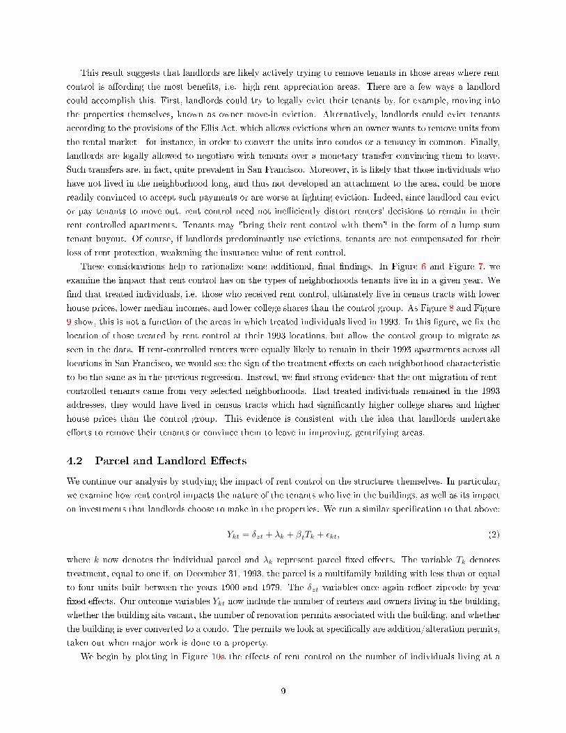
These considerations help to rationalize some additional, �nal �ndings. In Figure 6 and Figure 7, we

examine the impact that rent control has on the types of neighborhoods tenants live in in a given year. We

�nd that treated individuals, i.e. those who received rent control, ultimately live in census tracts with lower

house prices, lower median incomes, and lower college shares than the control group. As Figure 8 and Figure

9 show, this is not a function of the areas in which treated individuals lived in 1993. In this �gure, we �x the

location of those treated by rent control at their 1993 locations, but allow the control group to migrate as

seen in the data. If rent-controlled renters were equally likely to remain in their 1993 apartments across all

locations in San Francisco, we would see the sign of the treatment e�ects on each neighborhood characteristic

to be the same as in the previous regression. Instead, we �nd strong evidence that the out-migration of rent-

controlled tenants came from very selected neighborhoods. Had treated individuals remained in the 1993

addresses, they would have lived in census tracts which had signi�cantly higher college shares and higher

house prices than the control group. This evidence is consistent with the idea that landlords undertake

e�orts to remove their tenants or convince them to leave in improving, gentrifying areas.

4.2 Parcel and Landlord E�ects

We continue our analysis by studying the impact of rent control on the structures themselves. In particular,

we examine how rent control impacts the nature of the tenants who live in the buildings, as well as its impact

on investments that landlords choose to make in the properties. We run a similar speci�cation to that above:

Ykt = δzt + λk + βtTk + εkt, (2)

where k now denotes the individual parcel and λk represent parcel �xed e�ects. The variable Tk denotes

treatment, equal to one if, on December 31, 1993, the parcel is a multifamily building with less than or equal

to four units built between the years 1900 and 1979. The δzt variables once again re�ect zipcode by year

�xed e�ects. Our outcome variables Ykt now include the number of renters and owners living in the building,

whether the building sits vacant, the number of renovation permits associated with the building, and whether

the building is ever converted to a condo. The permits we look at speci�cally are addition/alteration permits,

taken out when major work is done to a property.

We begin by plotting in Figure 10a the e�ects of rent control on the number of individuals living at a

9

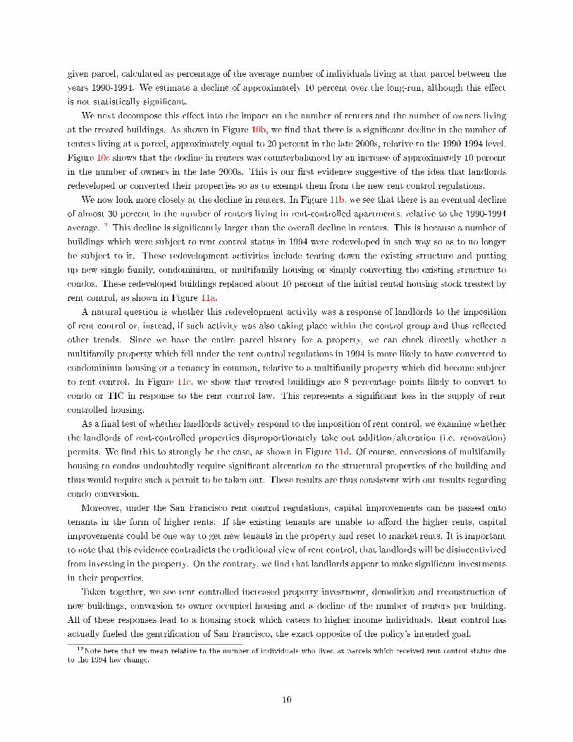
given parcel, calculated as percentage of the average number of individuals living at that parcel between the

years 1990-1994. We estimate a decline of approximately 10 percent over the long-run, although this e�ect

is not statistically signi�cant.

We next decompose this e�ect into the impact on the number of renters and the number of owners living

at the treated buildings. As shown in Figure 10b, we �nd that there is a signi�cant decline in the number of

renters living at a parcel, approximately equal to 20 percent in the late 2000s, relative to the 1990-1994 level.

Figure 10c shows that the decline in renters was counterbalanced by an increase of approximately 10 percent

in the number of owners in the late 2000s. This is our �rst evidence suggestive of the idea that landlords

redeveloped or converted their properties so as to exempt them from the new rent control regulations.

We now look more closely at the decline in renters. In Figure 11b, we see that there is an eventual decline

of almost 30 percent in the number of renters living in rent-controlled apartments, relative to the 1990-1994

average.12 This decline is signi�cantly larger than the overall decline in renters. This is because a number of

buildings which were subject to rent control status in 1994 were redeveloped in such way so as to no longer

be subject to it. These redevelopment activities include tearing down the existing structure and putting

up new single family, condominium, or multifamily housing or simply converting the existing structure to

condos. These redeveloped buildings replaced about 10 percent of the initial rental housing stock treated by

rent control, as shown in Figure 11a.

A natural question is whether this redevelopment activity was a response of landlords to the imposition

of rent control or, instead, if such activity was also taking place within the control group and thus re�ected

other trends. Since we have the entire parcel history for a property, we can check directly whether a

multifamily property which fell under the rent control regulations in 1994 is more likely to have converted to

condominium housing or a tenancy in common, relative to a multifamily property which did become subject

to rent control. In Figure 11c, we show that treated buildings are 8 percentage points likely to convert to

condo or TIC in response to the rent control law. This represents a signi�cant loss in the supply of rent

controlled housing.

As a �nal test of whether landlords actively respond to the imposition of rent control, we examine whether

the landlords of rent-controlled properties disproportionately take out addition/alteration (i.e. renovation)

permits. We �nd this to strongly be the case, as shown in Figure 11d. Of course, conversions of multifamily

housing to condos undoubtedly require signi�cant alteration to the structural properties of the building and

thus would require such a permit to be taken out. These results are thus consistent with our results regarding

condo conversion.

Moreover, under the San Francisco rent control regulations, capital improvements can be passed onto

tenants in the form of higher rents. If the existing tenants are unable to a�ord the higher rents, capital

improvements could be one way to get new tenants in the property and reset to market rents. It is important

to note that this evidence contradicts the traditional view of rent control, that landlords will be disincentivized

from investing in the property. On the contrary, we �nd that landlords appear to make signi�cant investments

in their properties.

Taken together, we see rent controlled increased property investment, demolition and reconstruction of

new buildings, conversion to owner occupied housing and a decline of the number of renters per building.

All of these responses lead to a housing stock which caters to higher income individuals. Rent control has

actually fueled the gentri�cation of San Francisco, the exact opposite of the policy's intended goal.

12Note here that we mean relative to the number of individuals who lived at parcels which received rent control status dueto the 1994 law change.

10

5 A Structural Spatial Equilibrium Model

The reduced form shows that rent control can either increase or decreases tenancy durations depending

on whether the tenant receives a buyout or eviction or instead remains at their residence at below market

rents. To quantify how tenants trade o� these decisions and to quantify the welfare impact of rent control

to covered tenants, we estimate a dynamic discrete choice model of neighborhood choice.

5.1 Model Setup

Each year t, a household decides whether to remain in its current home, a choice which we denote as S, orto move, in which case the households chooses a neighborhood j ∈ J to live in. We denote the household's

choice as x ∈ {S} ∪ J . The relevant state variables for the household's decision problem are the current

neighborhood jt−1 ∈ J , the number of years lived in the current neighborhood τn,t−1 ∈ N∪{0} , the numberof years lived in the current house τh,t−1 ∈ N∪{0}, and whether the residence is rent-controlled dt−1 ∈ {0, 1} .We also have a state variable at−1 ∈ {Y,M} denoting whether the household is in a young (Y ) or mature

(M) state of life. We let θt−1 = (jt−1, τn,t−1, τh,t−1, dt−1, at−1) denote the household's current state variable.

The transition dynamics of the state variable are straightforward. We have jt = j (xt), where:

j (xt) = jt−1 if xt = S

j (xt) = xt otherwise.

This equation simply says that the neighborhood remains the same if the household decides to remain in its

current home. Otherwise, the new neighborhood is given by the household's choice. The implications for

years in the current neighborhood and years in the current house are clearly similar, with:

τn (xt) = τn,t−1 + 1 if xt ∈ {S, jt−1}

τn (xt) = 0 otherwise.

and

τh (xt) = τh,t−1 + 1 if xt = S

τn (xt) = 0 otherwise.

Finally, we assume that each period young households transition to mature households with exogenous

probability ξ. This is clearly a simpli�cation, made due to limitations of the data, but captures the idea that

households experience certain life events such as marriage and having children at di�erent ages.13 Mature

households do not transition back into young households. We denote the (probabilistic) transition function

as θt = Θ (xt, θt−1) . We identify the set of neighborhood locations J as the San Francisco zipcodes, the

counties (other than San Francisco County) in the Bay Area, and an outside option denoting any location

outside of the Bay Area.

13In principle, we could tract the exact age as a stage variable, but this makes the state space very large.

11

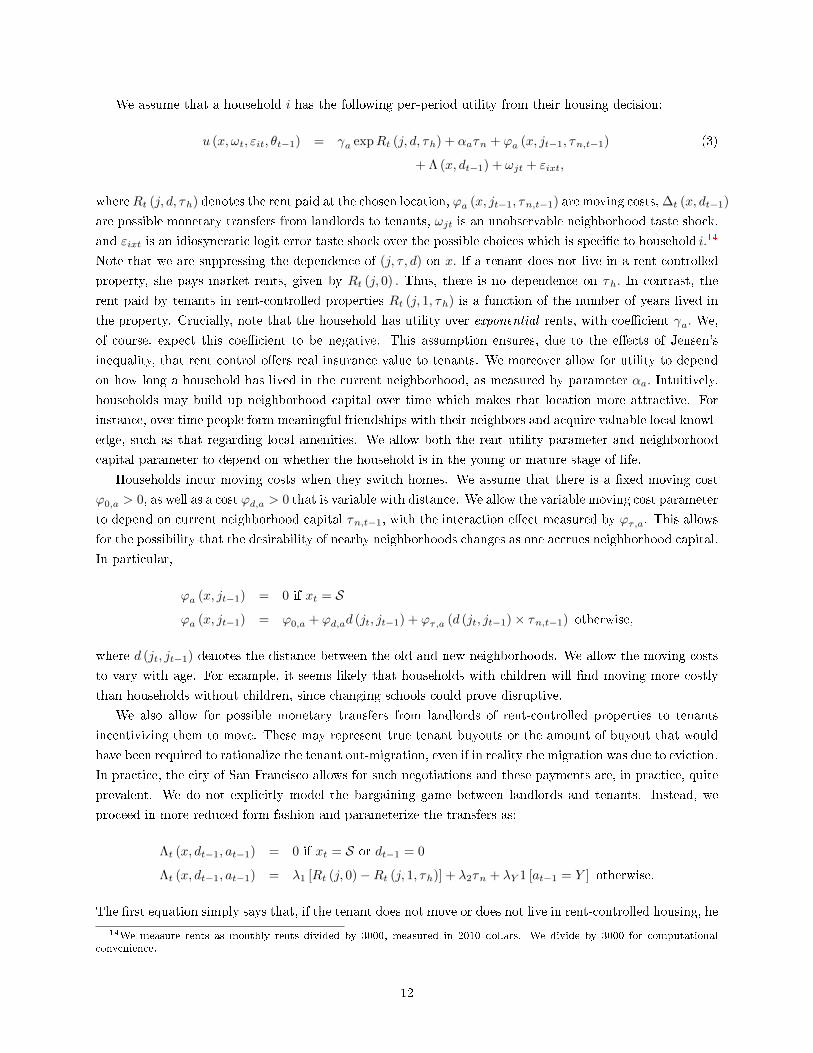
We assume that a household i has the following per-period utility from their housing decision:

u (x, ωt, εit, θt−1) = γa expRt (j, d, τh) + αaτn + ϕa (x, jt−1, τn,t−1) (3)

+ Λ (x, dt−1) + ωjt + εixt,

whereRt (j, d, τh) denotes the rent paid at the chosen location, ϕa (x, jt−1, τn,t−1) are moving costs, ∆t (x, dt−1)

are possible monetary transfers from landlords to tenants, ωjt is an unobservable neighborhood taste shock,

and εixt is an idiosyncratic logit error taste shock over the possible choices which is speci�c to household i.14

Note that we are suppressing the dependence of (j, τ , d) on x. If a tenant does not live in a rent-controlled

property, she pays market rents, given by Rt (j, 0) . Thus, there is no dependence on τh. In contrast, the

rent paid by tenants in rent-controlled properties Rt (j, 1, τh) is a function of the number of years lived in

the property. Crucially, note that the household has utility over exponential rents, with coe�cient γa. We,

of course, expect this coe�cient to be negative. This assumption ensures, due to the e�ects of Jensen's

inequality, that rent control o�ers real insurance value to tenants. We moreover allow for utility to depend

on how long a household has lived in the current neighborhood, as measured by parameter αa. Intuitively,

households may build up neighborhood capital over time which makes that location more attractive. For

instance, over time people form meaningful friendships with their neighbors and acquire valuable local knowl-

edge, such as that regarding local amenities. We allow both the rent utility parameter and neighborhood

capital parameter to depend on whether the household is in the young or mature stage of life.

Households incur moving costs when they switch homes. We assume that there is a �xed moving cost

ϕ0,a > 0, as well as a cost ϕd,a > 0 that is variable with distance. We allow the variable moving cost parameter

to depend on current neighborhood capital τn,t−1, with the interaction e�ect measured by ϕτ,a. This allows

for the possibility that the desirability of nearby neighborhoods changes as one accrues neighborhood capital.

In particular,

ϕa (x, jt−1) = 0 if xt = S

ϕa (x, jt−1) = ϕ0,a + ϕd,ad (jt, jt−1) + ϕτ,a (d (jt, jt−1)× τn,t−1) otherwise,

where d (jt, jt−1) denotes the distance between the old and new neighborhoods. We allow the moving costs

to vary with age. For example, it seems likely that households with children will �nd moving more costly

than households without children, since changing schools could prove disruptive.

We also allow for possible monetary transfers from landlords of rent-controlled properties to tenants

incentivizing them to move. These may represent true tenant buyouts or the amount of buyout that would

have been required to rationalize the tenant out-migration, even if in reality the migration was due to eviction.

In practice, the city of San Francisco allows for such negotiations and these payments are, in practice, quite

prevalent. We do not explicitly model the bargaining game between landlords and tenants. Instead, we

proceed in more reduced form fashion and parameterize the transfers as:

Λt (x, dt−1, at−1) = 0 if xt = S or dt−1 = 0

Λt (x, dt−1, at−1) = λ1 [Rt (j, 0)−Rt (j, 1, τh)] + λ2τn + λY 1 [at−1 = Y ] otherwise.

The �rst equation simply says that, if the tenant does not move or does not live in rent-controlled housing, he

14We measure rents as monthly rents divided by 3000, measured in 2010 dollars. We divide by 3000 for computationalconvenience.

12

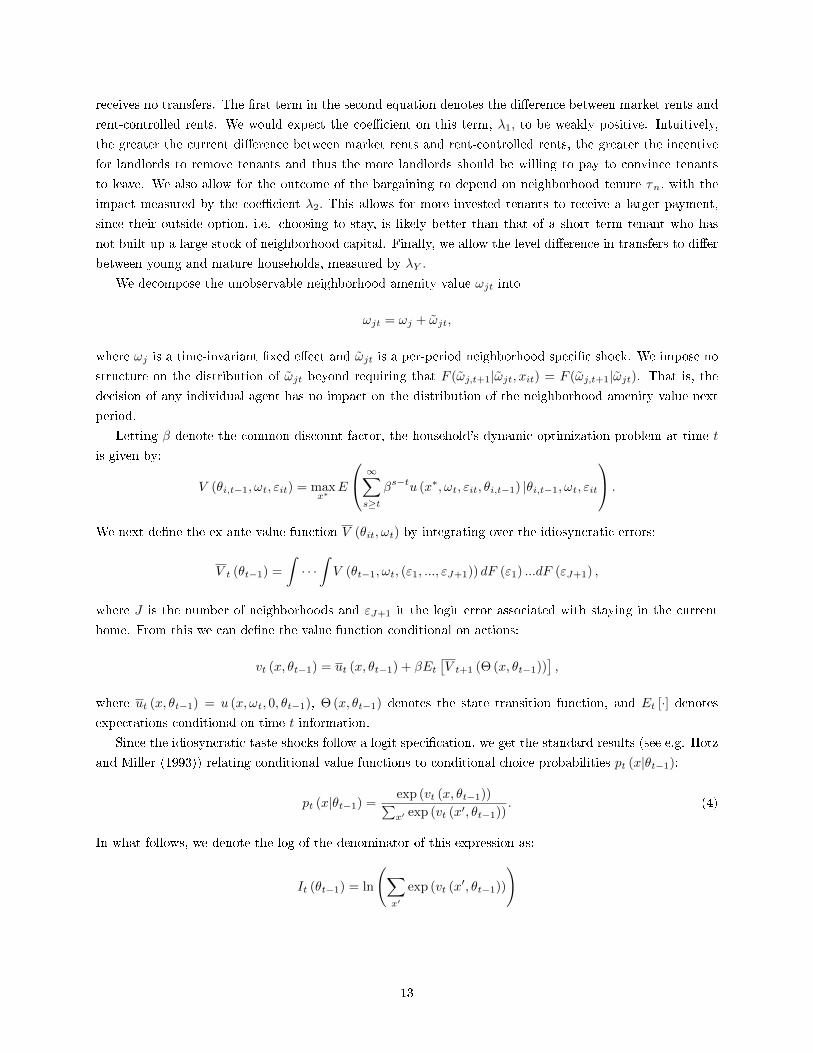
receives no transfers. The �rst term in the second equation denotes the di�erence between market rents and

rent-controlled rents. We would expect the coe�cient on this term, λ1, to be weakly positive. Intuitively,

the greater the current di�erence between market rents and rent-controlled rents, the greater the incentive

for landlords to remove tenants and thus the more landlords should be willing to pay to convince tenants

to leave. We also allow for the outcome of the bargaining to depend on neighborhood tenure τn, with the

impact measured by the coe�cient λ2. This allows for more invested tenants to receive a larger payment,

since their outside option, i.e. choosing to stay, is likely better than that of a short term tenant who has

not built up a large stock of neighborhood capital. Finally, we allow the level di�erence in transfers to di�er

between young and mature households, measured by λY .

We decompose the unobservable neighborhood amenity value ωjt into

ωjt = ωj + ω̃jt,

where ωj is a time-invariant �xed e�ect and ω̃jt is a per-period neighborhood speci�c shock. We impose no

structure on the distribution of ω̃jt beyond requiring that F (ω̃j,t+1|ω̃jt, xit) = F (ω̃j,t+1|ω̃jt). That is, the

decision of any individual agent has no impact on the distribution of the neighborhood amenity value next

period.

Letting β denote the common discount factor, the household's dynamic optimization problem at time t

is given by:

V (θi,t−1, ωt, εit) = maxx∗

E

∞∑s≥t

βs−tu (x∗, ωt, εit, θi,t−1) |θi,t−1, ωt, εit

.

We next de�ne the ex-ante value function V (θit, ωt) by integrating over the idiosyncratic errors:

V t (θt−1) =

∫· · ·∫V (θt−1, ωt, (ε1, ..., εJ+1)) dF (ε1) ...dF (εJ+1) ,

where J is the number of neighborhoods and εJ+1 it the logit error associated with staying in the current

home. From this we can de�ne the value function conditional on actions:

vt (x, θt−1) = ut (x, θt−1) + βEt[V t+1 (Θ (x, θt−1))

],

where ut (x, θt−1) = u (x, ωt, 0, θt−1), Θ (x, θt−1) denotes the state transition function, and Et [·] denotesexpectations conditional on time t information.

Since the idiosyncratic taste shocks follow a logit speci�cation, we get the standard results (see e.g. Hotz

and Miller (1993)) relating conditional value functions to conditional choice probabilities pt (x|θt−1):

pt (x|θt−1) =exp (vt (x, θt−1))∑x′ exp (vt (x′, θt−1))

. (4)

In what follows, we denote the log of the denominator of this expression as:

It (θt−1) = ln

(∑x′

exp (vt (x′, θt−1))

)

13

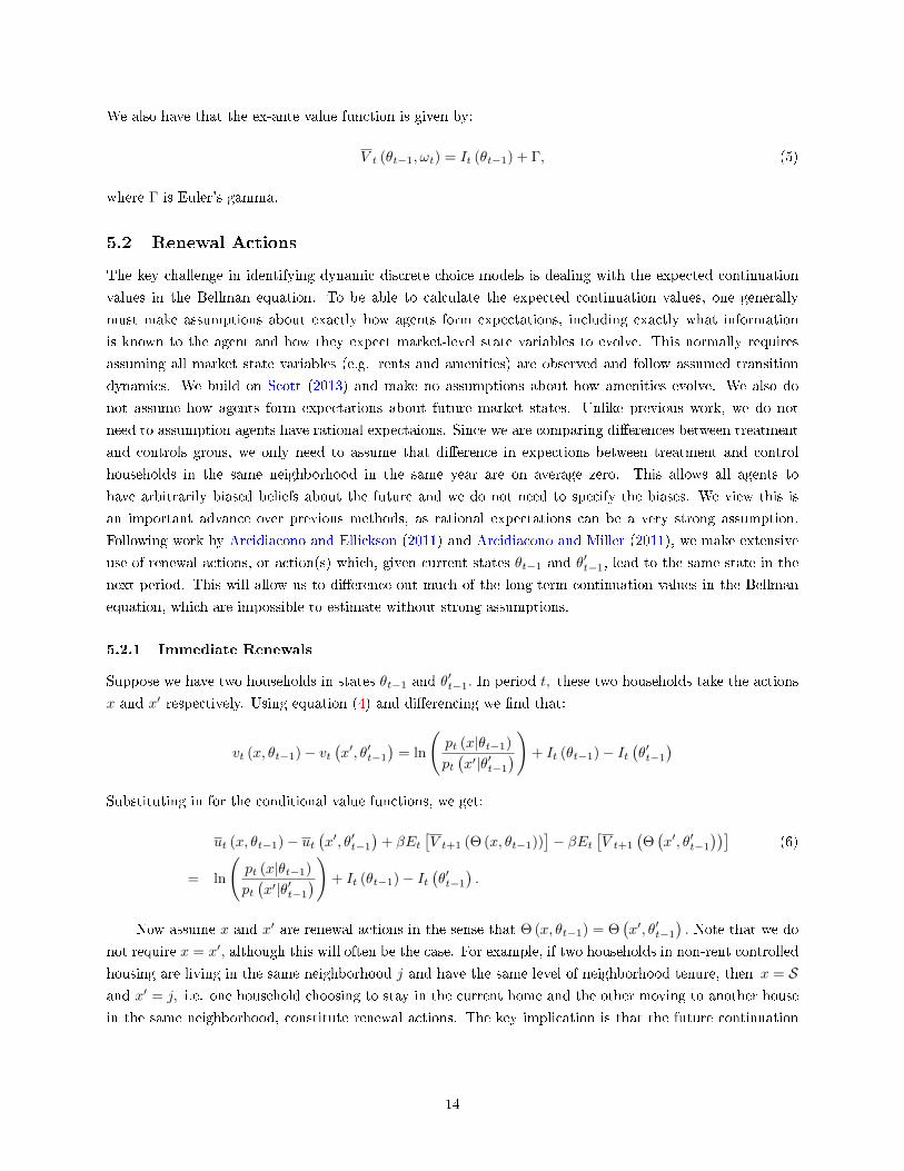
We also have that the ex-ante value function is given by:

V t (θt−1, ωt) = It (θt−1) + Γ, (5)

where Γ is Euler's gamma.

5.2 Renewal Actions

The key challenge in identifying dynamic discrete choice models is dealing with the expected continuation

values in the Bellman equation. To be able to calculate the expected continuation values, one generally

must make assumptions about exactly how agents form expectations, including exactly what information

is known to the agent and how they expect market-level state variables to evolve. This normally requires

assuming all market state variables (e.g. rents and amenities) are observed and follow assumed transition

dynamics. We build on Scott (2013) and make no assumptions about how amenities evolve. We also do

not assume how agents form expectations about future market states. Unlike previous work, we do not

need to assumption agents have rational expectaions. Since we are comparing di�erences between treatment

and controls grous, we only need to assume that di�erence in expections between treatment and control

households in the same neighborhood in the same year are on average zero. This allows all agents to

have arbitrarily biased beliefs about the future and we do not need to specify the biases. We view this is

an important advance over previous methods, as rational expectations can be a very strong assumption.

Following work by Arcidiacono and Ellickson (2011) and Arcidiacono and Miller (2011), we make extensive

use of renewal actions, or action(s) which, given current states θt−1 and θ′t−1, lead to the same state in the

next period. This will allow us to di�erence out much of the long-term continuation values in the Bellman

equation, which are impossible to estimate without strong assumptions.

5.2.1 Immediate Renewals

Suppose we have two households in states θt−1 and θ′t−1. In period t, these two households take the actions

x and x′ respectively. Using equation (4) and di�erencing we �nd that:

vt (x, θt−1)− vt(x′, θ′t−1

)= ln

(pt (x|θt−1)

pt(x′|θ′t−1

))+ It (θt−1)− It(θ′t−1

)Substituting in for the conditional value functions, we get:

ut (x, θt−1)− ut(x′, θ′t−1

)+ βEt

[V t+1 (Θ (x, θt−1))

]− βEt

[V t+1

(Θ(x′, θ′t−1

))](6)

= ln

(pt (x|θt−1)

pt(x′|θ′t−1

))+ It (θt−1)− It(θ′t−1

).

Now assume x and x′ are renewal actions in the sense that Θ (x, θt−1) = Θ(x′, θ′t−1

). Note that we do

not require x = x′, although this will often be the case. For example, if two households in non-rent controlled

housing are living in the same neighborhood j and have the same level of neighborhood tenure, then x = Sand x′ = j, i.e. one household choosing to stay in the current home and the other moving to another house

in the same neighborhood, constitute renewal actions. The key implication is that the future continuation

14

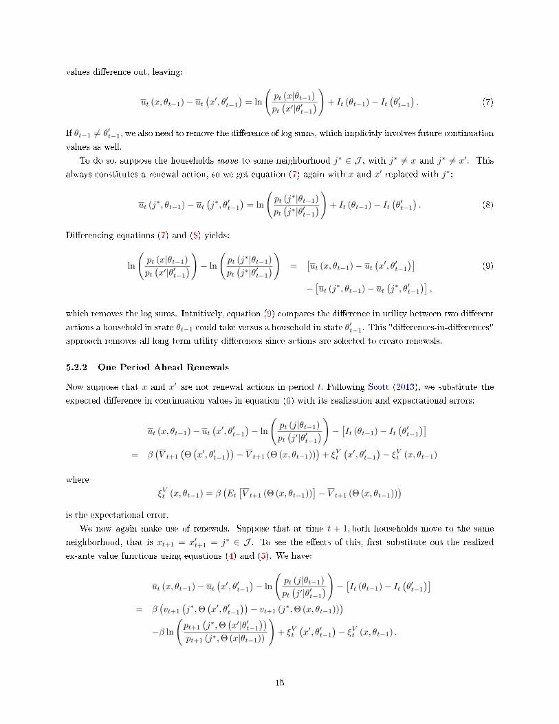
values di�erence out, leaving:

ut (x, θt−1)− ut(x′, θ′t−1

)= ln

(pt (x|θt−1)

pt(x′|θ′t−1

))+ It (θt−1)− It(θ′t−1

). (7)

If θt−1 6= θ′t−1, we also need to remove the di�erence of log sums, which implicitly involves future continuation

values as well.

To do so, suppose the households move to some neighborhood j∗ ∈ J , with j∗ 6= x and j∗ 6= x′. This

always constitutes a renewal action, so we get equation (7) again with x and x′ replaced with j∗:

ut (j∗, θt−1)− ut(j∗, θ′t−1

)= ln

(pt (j∗|θt−1)

pt(j∗|θ′t−1

))+ It (θt−1)− It(θ′t−1

). (8)

Di�erencing equations (7) and (8) yields:

ln

(pt (x|θt−1)

pt(x′|θ′t−1

))− ln

(pt (j∗|θt−1)

pt(j∗|θ′t−1

)) =[ut (x, θt−1)− ut

(x′, θ′t−1

)](9)

−[ut (j∗, θt−1)− ut

(j∗, θ′t−1

)],

which removes the log sums. Intuitively, equation (9) compares the di�erence in utility between two di�erent

actions a household in state θt−1 could take versus a household in state θ′t−1. This "di�erences-in-di�erences"

approach removes all long-term utility di�erences since actions are selected to create renewals.

5.2.2 One Period Ahead Renewals

Now suppose that x and x′ are not renewal actions in period t. Following Scott (2013), we substitute the

expected di�erence in continuation values in equation (6) with its realization and expectational errors:

ut (x, θt−1)− ut(x′, θ′t−1

)− ln

(pt (j|θt−1)

pt(j′|θ′t−1

))− [It (θt−1)− It(θ′t−1

)]= β

(V t+1

(Θ(x′, θ′t−1

))− V t+1 (Θ (x, θt−1))

)+ ξVt

(x′, θ′t−1

)− ξVt (x, θt−1)

where

ξVt (x, θt−1) = β(Et[V t+1 (Θ (x, θt−1))

]− V t+1 (Θ (x, θt−1))

)is the expectational error.

We now again make use of renewals. Suppose that at time t + 1, both households move to the same

neighborhood, that is xt+1 = x′t+1 = j∗ ∈ J . To see the e�ects of this, �rst substitute out the realized

ex-ante value functions using equations (4) and (5). We have:

ut (x, θt−1)− ut(x′, θ′t−1

)− ln

(pt (j|θt−1)

pt(j′|θ′t−1

))− [It (θt−1)− It(θ′t−1

)]= β

(vt+1

(j∗,Θ

(x′, θ′t−1

))− vt+1 (j∗,Θ (x, θt−1))

)−β ln

(pt+1

(j∗,Θ

(x′|θ′t−1

))pt+1 (j∗,Θ (x|θt−1))

)+ ξVt

(x′, θ′t−1

)− ξVt (x, θt−1) .

15

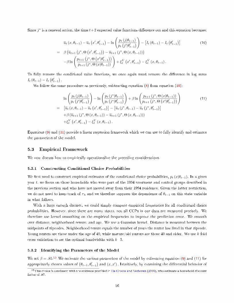
Since j∗ is a renewal action, the time t+2 expected value functions di�erence out and this equation becomes:

ut (x, θt−1)− ut(x′, θ′t−1

)− ln

(pt (j|θt−1)

pt(j′|θ′t−1

))− [It (θt−1)− It(θ′t−1

)](10)

= β(ut+1

(j∗,Θ

(x′, θ′t−1

))− ut+1 (j∗,Θ (x, θt−1))

)−β ln

(pt+1

(j∗,Θ

(x′|θ′t−1

))pt+1 (j∗,Θ (x|θt−1))

)+ ξVt

(x′, θ′t−1

)− ξVt (x, θt−1) .

To fully remove the conditional value functions, we once again must remove the di�erence in log sums

It (θt−1)− It(θ′t−1

).

We follow the same procedure as previously, subtracting equation (8) from equation (10):

ln

(pt (j|θt−1)

pt(j′|θ′t−1

))− ln

(pt (j∗|θt−1)

pt(j∗|θ′t−1

))+ β ln

(pt+1 (j∗,Θ (x|θt−1))

pt+1

(j∗,Θ

(x′|θ′t−1

))) (11)

=[ut (x, θt−1)− ut

(x′, θ′t−1

)]−[ut (j∗, θt−1)− ut

(j∗, θ′t−1

)]+β (ut+1 (j∗,Θ (x, θt−1))− ut+1 (j∗,Θ (x, θt−1)))

+ξVt(x′, θ′t−1

)− ξVt (x, θt−1) .

Equations (9) and (11) provide a linear regression framework which we can use to fully identify and estimate

the parameters of the model.

5.3 Empirical Framework

We now discuss how to empirically operationalize the preceding considerations.

5.3.1 Constructing Conditional Choice Probabilities

We �rst need to construct empirical estimates of the conditional choice probabilities, pt (x|θt−1). In a given

year t, we focus on those households who were part of the 1994 treatment and control groups described in

the previous section and who have not moved away from their 1994 residence. Given the latter restriction,

we do not need to keep track of τh and we therefore suppress the dependence of θt−1 on this state variable

in what follows.

With a large enough dataset, we could simply compute empirical frequencies for all conditional choice

probabilities. However, since there are many states, not all CCPs in our data are measured precisely. We

therefore use kernel smoothing on the empirical frequencies to improve the prediction error. We smooth

over distance, neighborhood tenure, and age. We use a Gaussian kernel. Distance is measured between the

midpoints of zipcodes. Neighborhood tenure equals the number of years the renter has lived in that zipcode.

Young renters are those under the age of 40, while mature/old renters are those 40 and older. We use k-fold

cross validation to set the optimal bandwidths with k=5.

5.3.2 Identifying the Parameters of the Model

We set β = .85.15 We estimate the various parameters of the model by estimating equation (9) and (11) for

appropriately chosen values of(θt−1, θ

′t−1)and (x, x′) . Intuitively, by examining the di�erential behavior of

15This choice is consistent with the evidence provided in De Groote and Verboven (2016), who estimate a household discountfactor of .87.

16

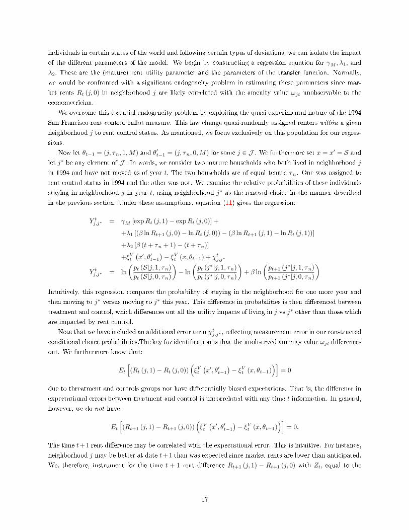
individuals in certain states of the world and following certain types of deviations, we can isolate the impact

of the di�erent parameters of the model. We begin by constructing a regression equation for γM , λ1, and

λ2. These are the (mature) rent utility parameter and the parameters of the transfer function. Normally,

we would be confronted with a signi�cant endogeneity problem in estimating these parameters since mar-

ket rents Rt (j, 0) in neighborhood j are likely correlated with the amenity value ωjt unobservable to the

econometrician.

We overcome this essential endogeneity problem by exploiting the quasi-experimental nature of the 1994

San Francisco rent control ballot measure. This law change quasi-randomly assigned renters within a given

neighborhood j to rent control status. As mentioned, we focus exclusively on this population for our regres-

sions.

Now let θt−1 = (j, τn, 1,M) and θ′t−1 = (j, τn, 0,M) for some j ∈ J . We furthermore set x = x′ = S and

let j∗ be any element of J . In words, we consider two mature households who both lived in neighborhood j

in 1994 and have not moved as of year t. The two households are of equal tenure τn. One was assigned to

rent control status in 1994 and the other was not. We examine the relative probabilities of these individuals

staying in neighborhood j in year t, using neighborhood j∗ as the renewal choice in the manner described

in the previous section. Under these assumptions, equation (11) gives the regression:

Y tj,j∗ = γM [expRt (j, 1)− expRt (j, 0)] +

+λ1 [(β lnRt+1 (j, 0)− lnRt (j, 0))− (β lnRt+1 (j, 1)− lnRt (j, 1))]

+λ2 [β (t+ τn + 1)− (t+ τn)]

+ξVt(x′, θ′t−1

)− ξVt (x, θt−1) + χtj,j∗

Y tj,j∗ = ln

(pt (S|j, 1, τn)

pt (S|j, 0, τn)

)− ln

(pt (j∗|j, 1, τn)

pt (j∗|j, 0, τn)

)+ β ln

(pt+1 (j∗|j, 1, τn)

pt+1 (j∗|j, 0, τn)

)Intuitively, this regression compares the probability of staying in the neighborhood for one more year and

then moving to j∗ versus moving to j∗ this year. This di�erence in probabilities is then di�erenced between

treatment and control, which di�erences out all the utility impacts of living in j vs j∗ other than those which

are impacted by rent control.

Note that we have included an additional error term χtj,j∗ , re�ecting measurement error in our constructed

conditional choice probabilities.The key for identi�cation is that the unobserved amenity value ωjt di�erences

out. We furthermore know that:

Et

[(Rt (j, 1)−Rt (j, 0))

(ξVt(x′, θ′t−1

)− ξVt (x, θt−1)

)]= 0

due to threatment and controls groups not have di�erentially biased expectations. That is, the di�erence in

expectational errors between treatment and control is uncorrelated with any time t information. In general,

however, we do not have:

Et

[(Rt+1 (j, 1)−Rt+1 (j, 0))

(ξVt(x′, θ′t−1

)− ξVt (x, θt−1)

)]= 0.

The time t+1 rent di�erence may be correlated with the expectational error. This is intuitive. For instance,

neighborhood j may be better at date t+1 than was expected since market rents are lower than anticipated.

We, therefore, instrument for the time t + 1 rent di�erence Rt+1 (j, 1) − Rt+1 (j, 0) with Zt, equal to the

17

one-period lagged value Rt (j, 1)−Rt−1 (j, 0). Since Zt is in the time t information set, we have:

Et

[Zt

(ξVt(x′, θ′t−1

)− ξVt (x, θt−1)

)]= 0.

Thus, our exclusion restrictions are satis�ed and the parameters are identi�ed.

To identify the impact of tenure on utility αM , consider two mature households living in non-rent con-

trolled housing in neighborhood j, with di�erent levels of initial tenure, τn and τ ′n.Suppose both households

move to j∗ after one year. We thus have θt−1 = (j, τn, 0,M) and θ′t−1 = (j, τ ′n, 0,M) for some j ∈ J and

x = x′ = S. Then equation (11) becomes:

Y tj,j∗ = αM (τn − τ ′n) + ξVt(x′, θ′t−1

)− ξVt (x, θt−1) + χtj,j∗

Y tj,j∗ = ln

(pt (S|j, 0, τn)

pt (S|j, 0, τ ′n)

)− ln

(pt (j∗|j, 0, τn)

pt (j∗|j, 0, τ ′n)

)+ β ln

(pt+1 (j∗|j, 0, τn)

pt+1 (j∗|j, 0, τ ′n)

)Since both households live in non-rent controlled housing in the same neighborhood, they pay the same rents

and receive the same unobserved amenity value. Indeed, the only payo�-relevant di�erence between the two

populations is the number of years they have lived in the neighborhood. Thus, appropriately examining the

relative probabilities of staying in the neighborhood is informative of the importance of tenure on utility or,

in other words, of the magnitude of αM . Intuitively, as one builds up more neighborhood capital, the bene�ts

of staying in the neighborhood an additional year. Thus, the relative probability of staying one more year

versus moving away should grow if neighborhood capital is accruing.

To estimate moving costs, we consider two mature households of equal tenure τn living in non-rent

controlled housing in neighborhood j. Suppose that one household immediately moves to another house in

the same zipcode and one household stays in the same home. Formally, θt−1 = θ′t−1 = (j, τn, 0,M), x =

S, and x′ = j. As was discussed in Section 5.2.1, this constitutes an immediate renewal since rents do not

change and neighborhood tenure does not change. Since one is only changing the house they live in due to

the logit error and the moving costs, we can identify the �xed cost of moving. If people move houses a lot

within a zipcode, moving costs must be low. If they do it rarely, moving costs must be high. Equation (9)

gives the regression:

Y tj = −ϕ0,M +χtj

Y tj = ln

(pt (S|j, 0, τn)

pt (j|j, 0, τn)

),

which identi�es the �xed moving cost parameter ϕ0,M . Note that there is only one log di�erence instead of

two since the households begin in the same state.

We also need the variable moving cost parameter, ϕd,M . Consider two mature households of equal tenure

τn, both living in non-rent controlled housing, one living in neighborhood j and the other in neighborhood

j′. Suppose they immediately move to either neighborhood j∗ or j∗∗. Both of these are choices constitute

immediate renewals. Therefore, Equation (9) gives the speci�cation:

Y tj,j′,j∗,j∗∗ = ϕd,M (dj,j∗ − dj′,j∗)− ϕd,M (dj,j∗∗ − dj′,j∗∗) + χtj,j′,j∗,j∗∗

Y tj,j′,j∗,j∗∗ = ln

(pt (j∗|j, 0, τn)

pt (j∗|j′, 0, τn)

)− ln

(pt (j∗∗|j, 0, τn)

pt (j∗∗|j′, 0, τn)

).

Intuitively, this compares the relative probabilities of moving to j∗ vs j∗∗ depending on whether one starts

18

in j or j′. If j is very close to j∗, but far from j∗∗, then the di�erence in moving costs between the moves in

large. However, if j′ is equidistant between the two, the moving costs between the two locations are the same.

The relationship between these di�erences in distances and di�erences in migration probabilities identi�es

the marginal cost of moving with respect to distance. Using similar considerations, one can estimate the

interaction term parameter ϕτ,M . The equation is detailed in the appendix.

As one would expect, the equations for young households are very similar to the ones described above,

but the probability of transitioning to a mature household must be taken into account. Furthermore, one

can use the treatment group as well as the control group to estimate the neighborhood tenure parameters

and the variable moving cost parameters. All of these additional equations are detailed in the appendix.

The model is then estimated via GMM.

Finally, it remains to estimate the permanent component of amenities ωj .16 We do so after estimating

the full GMM system detailed above. We once again consider two mature households of equal tenure τn,

living in neighborhoods j and j′ respectively and suppose that both households move to some neighborhood

j∗ after one year. We thus have, θt−1 = (j, τn, 0,M) , θ′t−1 = (j′, τn, 0,M) , and x = x′ = S. These choicesyield the equation:

Y tj,j′,j∗ = ωj − ωj′ + ω̃jt − ω̃j′t + ξVt(x′, θ′t−1

)− ξVt (x, θt−1) + χtj,j′,j∗

Y tj,j′,j∗ = ln

(pt (S|j, 0, τn)

pt (S|j′, 0, τn)

)− ln

(pt (j∗|j, 0, τn)

pt (j∗|j′, 0, τn)

)+ β ln

(pt+1 (j∗|j, 0, τn)

pt+1 (j∗|j′, 0, τn)

)− (β − 1)ϕd,M (dj,j∗ − dj′,j∗)− γM [Rt (j, 0)−Rt (j′, 0)]

Identi�cation comes from the fact that, averaging over time, we average out the per-period neighborhood

amenity shocks and expectational error shocks. Moreover, note that we do not have an endogeneity problem

since we have already estimated γM and can therefore move the utility impact of the rent di�erence to the

left hand side of the equation. We also account for the di�erential moving costs related to distance on the

left hand side of the equation. Finally, note that we can only identify �xed amenity value di�erences between

neighborhoods. We therefore choose a normalization, letting zipcode 94110, representing the Mission District

and Bernal Heights, be our baseline zipcode. We set its amenity value �xed e�ect to zero.

5.4 Model Estimates

Table 4 shows the parameter estimates of the model. Panel A reports the parameters measured in rent

equivalent dollar units, with the exception of the transfer payments, which are measured in actual dollar

amounts.17 Panel B reports the estimates in units of migration elasticities. We will focus on the estimates

in Panel A. Normalizing the coe�cient on exponential rents to 1, we identify the standard deviation of

tenants' idiosyncratic shocks to their location preferences. We �nd that young renters have annual location

taste shocks with a standard deviation equivalent to $7,411. Mature renters face location shocks with a

12.7% lower standard deviation. These estimates are consistent with our previously discussed hypothesis

that young renters' migration decisions are more driven by idiosyncratic shocks than older households.

Turning to the magnitudes of the tenant buyouts, we �nd young renters receive $1.631 more dollars

from their landlords for each additional $1 below market their rent is. Mature renters face similar impact of

$1.404. We also �nd buyout o�ers are larger as tenants live in their zipcodes longer. For each additional year

16We cannot identify amenities of the outside options, i.e. the rest of the Bay Area and the rest of the country, as no one inour 1994 cohorts started o� living in those locations.

17These are measured at the mean rent paid by rent-controlled households, $2350.

19

a young (mature) tenant lives in their zipcode, they receive $164 ($141) additional dollars in the buyout o�er

from their landlord. Finally, we �nd mature tenants receive larger buyout o�ers overall by $70,702. This

may re�ect that landlords expect older tenants to remain in their apartments for the very long term. Along

the same lines, to the extent that these transfers re�ect evictions, landlords would be more incentivized to

evict older renters. To get a better sense of the magnitudes of these buyout payments, Figure 13 plots the

average buyout to young tenants o�ered in each year in the data, across all tenants and neighborhoods. By

2010, the average o�er to tenants who still remain at their 1994 address is just over $30,000. Figure 14 plots

the heterogeneity across zipcodes in mean buyout o�ers, highlighting that some zipcodes experience much

larger rent increases than others over this time period. In the most expensive zipcode, the average buyout

in 2010 is just about $40,000, while in the cheapest zipcode the mean buyout o�er is around $25,000. These

numbers seem very much in line with popular press anecdotes about tenant buyouts in San Francisco.

Moving along to our estimates of moving costs, we �nd the �xed cost of moving is equivalent, in rent-

equivalent dollars, to $42,626 for young renters and $38,988 for old renters. These estimates seem quite

reasonable and actually quite below what is typically found in the literature. A main driver of the magnitude

of this estimate are the short-run migration elasticities with respect to a one-year temporary change. It is

often quite hard to �nd a high quality instrument for rents that does not e�ect other omitted variables such

as amenities. Likely, many instruments for rent also impact the supply and quality of amenities, leading to

rent elasticities being biased towards 0. Our rent control policy experiment only a�ects rents and cannot

a�ect amenities in our regressions, as we are comparing migration decisions between market rent and rent

controlled households in the same neighborhood consuming the same amenities.

In addition to the �xed costs of moving, we �nd that the moving costs increase with the distance of

the move. A 1 percent increase in move distance is equivalent to $114 for the young and $101 for the old.

Finally, we also consider whether these variable moving costs change as households live in their zipcodes

longer. One might think that the longer a household has lived in the area the more familiar they are with

further and further away neighborhoods, lowering those marginal moving costs. Indeed, we �nd this is the

case, with each additional year a tenant has lived in their zipcode lowering the moving cost by $415 for the

young and $357 for the old.

Lastly, we turn to our neighborhood capital estimates. Proponents of rent control often argue that long-

term residents are the ones in the most need of rent control as migrating away from their community forces

them to lose many of the connections and investments they have been in the neighborhoods over time. We

do �nd very statistically signi�cant e�ects of neighborhood capital accumulation. However, the economic

magnitude is small. Young (mature) households increasingly value living in their zipcode by $266 ($292) in

dollar rent equivalent terms. However, these e�ects can add up to a sizable e�ect over a lifetime.

6 Welfare E�ects of Rent Control

6.1 Welfare Decomposition: 1994-2012

We begin our investigation of the welfare e�ects of rent control by decomposing the impacts of the 1994

ballot initiative on its bene�ciaries, relative to the control group. We discuss here mature households. The

expressions for young households are exactly analogous.

20

6.1.1 Derivations

In any given year t between the years of 1994 and 2012, the average utility di�erence between the treatment

group and the control group is given by:

∆UMt =∑θt−1

∑x

(ut (x, θt−1) + Et [εixt|x, θt−1]) pt (x|θt−1)(pTt (θt−1)− pCt (θt−1)

)(12)

=∑θt−1

∑x

(ut (x, θt−1) + Et [εixt|x, θt−1])(pTt (x, θt−1)− pCt (x, θt−1)

)where recall ut (x, θt−1) = u (x, ωt, 0, θt−1) and the utility function is de�ned in equation (3). The expression

pt (x|θt−1) again denotes the conditional probability of choosing x ∈ {S}∪J , given that the current state is

θt−1, pTt (θt−1) , pCt (θt−1) denote the probabilities of being in state θt−1 for the treatment group and control

group respectively, and pTt (x, θt−1) , pCt (x, θt−1) denote the joint probabilities. The conditional expectation

Et [εit|x, θt−1] denotes the expected logit error conditional on choosing x from state θt−1. Of course, equation

(12) simply says that the average utility di�erence is the weighted average utility received by the treatment

group minus the weighted average utility received by the control group.

We can decompose this average utility di�erence by substituting in for the utility function from equation

(3). We �nd that:

∆UMt = ∆UM,Rentt + ∆UM,Payoff

t + ∆UM,NCt (13)

+∆UM,MCt + ∆UM,Miles

t + ∆UM,Amenityt + ∆UM,Logit

t .

That is, the average utility di�erence between the treatment group and the control arises from di�erences in

average rent paid ∆UM,Rentt , in transfers received from landlords ∆UM,Payoff

t , in accumulated neighborhood

capital ∆UM,NCt , in �xed costs ∆UM,MC

t , in variable moving costs ∆UM,Milest , in neighborhood amenity

values ∆UM,Amenityt , and in idiosyncratic valuations ∆UM,Logit

t . Suppressing the dependence of j and τ on

x, we can formally write these terms as:

∆URentt =

∑θt−1

∑x

γM exp (Rt (j, d, τh))(pTt (x, θt−1)− pCt (x, θt−1)

)∆UPayofft =

∑θt−1

∑x

Λt (x, dt−1,M)(pTt (x, θt−1)− pCt (x, θt−1)

)∆UM,NC

t =∑θt−1

∑x

αMτn(pTt (x, θt−1)− pCt (x, θt−1)

)∆UM,MC

t =∑θt−1

∑x

ϕ0,M1 [x 6= S](pTt (x, θt−1)− pCt (x, θt−1)

)∆UM,Miles

t =∑θt−1

∑x

ϕd,Mdj,jt−11 [x 6= S]

(pTt (x, θt−1)− pCt (x, θt−1)

)∆UM,Amenity

t =∑θt−1

∑x

ωjt(pTt (x, θt−1)− pCt (x, θt−1)

).

We can measure each of these terms.18 We recover estimates of γM ,ΛM , αM , ϕ0,M , ϕd,M , and ωjt from our

structural model. We can then recover the other needed quantities from standard reduced form di�erences-

in-di�erences analysis. For example,

18Since we measure rents as monthly rents/3000, we multiply by 36,000 to convert to an annual rent number.

21

∑θt−1

∑x exp (Rt (j, d, τh))

(pTt (x, θt−1)− pCt (x, θt−1)

)is simply the average di�erence in rents paid be-

tween treatment and control in year t,∑θt−1

∑x τn

(pTt (x, θt−1)− pCt (x, θt−1)

)is the average di�erence in

accumulated neighborhood capital between treatment and control,∑θt−1

∑x 1 [x 6= S]

(pTt (x, θt−1)− pCt (x, θt−1)

)is the average di�erence in number of moves between treatment and control, and∑θt−1

∑x dj,jt−11 [x 6= S]

(pTt (x, θt−1)− pCt (x, θt−1)

)is the average di�erence in distance moved between

treatment and control. Each of these can be readily calculated using the reduced form methodology de-

scribed in Section 4. The average utility di�erence due to transfers and the average utility di�erence due to

amenities can be similarly calculated by combining our structural estimates with reduced form di�erences-

in-di�erences analysis.

Deriving an expression for the utility di�erence due to idiosyncratic valuations ∆UM,Logitt is a bit more

complicated. We have that:

∆UM,Logitt =

∑θt−1

∑x

Et [εit|x, θt−1](pTt (x, θt−1)− pCt (x, θt−1)

). (14)

We therefore need an expression for the conditional expectation Et [εixt|x, θt−1] . Using Bayes' rule, we get:

Et [εixt|x, θt−1] =

∫εixt

(∏x′ 6=x e

−e−(εixt+vt(x,θt−1)−vt(x′,θt−1))

)e−εixte−e

−εixtdεixt

pt (x|θt−1)

=

∫εixt

(∏x′ 6=x e

−e−(εixt+ln pt(x|θt−1)−ln pt(x′|θt−1)))e−εixte−e

−εixtdεixt

pt (x|θt−1),

where in the second equality we used the Hotz and Miller (1993) inversion vt (x, θt−1) − vt (x′, θt−1) =

ln pt (x|θt−1)− ln pt (x′|θt−1) . Substituting into equation (14), we derive:

∆UM,Logitt =

∑θt−1

∑x

∫εixt

∏x′ 6=x

e−e−(εixt+ln pt(x|θt−1)−ln pt(x′|θt−1))

e−εixte−e−εixt

dεixt

×(pTt (θt−1)− pCt (θt−1)

).

(15)

Since we have empirical estimates of each of the probabilities, we can estimate this utility di�erence.

We �nally convert our estimated utility di�erences into rent equivalent dollar amounts. Consider an

individual in the control group who pays the average San Francisco rent in year t, which we denote as Rt.

We now proceed iteratively. The dollar rent equivalent ∆WRentt of the utility di�erence ∆URent

t in year t

due to rent di�erences can be calculated as the solution to :

γM exp(Rt + ∆WRent

t

)− γM exp

(Rt)

= ∆URentt ,

which gives:

∆WRentt = ln

(∆URent

t

γM+ exp

(Rt))−Rt.

The dollar rent equivalent incremental impact of transfers can then be calculated as:

∆WPayofft = ln

(∆UPayofft

γM+ exp

(Rt + ∆WRent

t

))−(Rt + ∆WRent

t

).

22

Now let ∆UM,ιt denote the utility di�erences, with ι ∈ {1, ..., 7} corresponding to the ordering in equation

(13). Iterating on our procedure gives the dollar rent equivalent incremental impacts of each element of the

decomposition:

∆W ιt = ln

(∆UPayofft

γM+ exp

(Rt +

∑ι′<ι

∆W ι′

t

))−

(Rt +

∑ι′<ι

∆W ι′

t

).

6.1.2 Results

The results of this decomposition are reported in Table 5. We �nd that the bene�ciaries of the 1994 rent

control law received large welfare bene�ts between the 1994-2012 period. Older households received a total

rent-equivalent dollar bene�t of $119,837, re�ecting an annual bene�t of $6,658. These bene�ts were front

loaded, with households earning a cumulative bene�t of $74,622 and average annual bene�t of $8,291 during

the 1995-2003 period Cumulative bene�ts equaled $45,216 during the 2004-2012 period, re�ecting an annual

average of $5,024.

In terms of decomposition, most of the bene�ts from the rent control law came from protection against

rent increases and transfers.19 Respectively, protection against rent increases constituted 44.2% of the total

bene�t and transfers constituted 30.1% of the total. Lower moving costs, both �xed and variable, were 13.5%

of the total. Increased neighborhood capital constituted only small fraction of the total bene�t at 1.2%. The

welfare bene�ts from increased amenity values were negligible. Interestingly, we �nd increased utility from

the utility value of one's idiosyncratic preference equal to 11.3% of the welfare gain. This likely due to the

fact that we found some low neighborhood capital households were more likely to move due to rent control,

allowing them to over come moving costs and live in a location that best suites their idiosyncratic preference.

The bene�ts of the rent control expansion were smaller for younger households, although still large. That

they are smaller is consistent with our estimate that younger households receive larger idiosyncratic shocks,

which leads to more frequent moving and thus smaller bene�ts from rent control protections. Younger

households are also estimated to receive smaller transfers. Cumulative welfare bene�ts for these households

totaled $41,121, re�ecting an annual average of $2,285. Similar to older households, the bene�ts were

front loaded. Younger households received cumulative bene�ts of $32,960 during the 1995-2003 period

and cumulative bene�ts of $8,162 during the 2004-2012 period. Annual averages were $3,662 and $907

respectively.

Also similar to older households, most of the bene�ts came from protection against rent increases and

transfers, constituting 79.6% and 45.4% respectively over the total period. The fraction due to moving costs

is much smaller for younger households, at only 8%. Note this reinforces the idea that, due to a higher

variance if idiosyncratic shocks, younger households optimally choose to move more often. The fraction due

to neighborhood capital is once again small, constituting just 2.6% for the average. Welfare bene�ts due to

increased amenity values now re�ect a small, but non-negligible, fraction of the total bene�t at 2.6%. Finally,

the young face a substantial welfare loss due to living in places that are worse matches to their idiosyncratic

preference under rent control, equal to -37.2%. This re�ects that to stay in one's apartment to bene�t from

below market rents, one must give up living in the best apartment and location that suites one's preferences.

19The model assumes that all observed moves are rational choices. The transfers we estimate are those which rationalizethe observed empirical frequencies. It is possible that some of the moves we see in the data are forced evictions, rather thanthe result of negotiations between landlords and tenants over monetary compensation. To the extent that this is the case, ourwelfare bene�ts from transfer payments over overstated. However, even in the extreme case where the welfare bene�ts fromtransfers are zero, the bene�ts from protection against rent increases would still be large.

23

Our estimates shows that idiosyncratic preference variance is higher for the young, making giving up the

match value a larger sacri�ce.

We aggregate these numbers over the entire population of renters impacted by the rent control law. The

aggregate welfare bene�ts are very large. Older households received a cumulative (undiscounted) bene�t of

$2.5 billion over the entire period, while younger households received a cumulative bene�t of $1.3 billion

dollars. Across the entire population, the aggregate bene�t was $3.9 billion dollars, re�ecting an annual

average of $214 million dollars. To put this in present discount value using a discount rate of 0.95, this

equates to a $2.9 billion dollar welfare gain to treated tenants. Note also that these welfare numbers are only

for the 1994 population impacted by the rent control expansion. It does not take into account the welfare

bene�ts for renters who moved into the impacted properties in later years, which presumably were also quite

large.

6.2 General Equilibrium Welfare Impact of Reduced Supply

We �nally turn to evaluating the GE welfare impact of the landlord supply response. Intuitively, since

landlords reduced supply in response to the 1994 law, as was shown in Section 4.2, average San Francisco

rents were higher than they otherwise would have been. Using our structural framework, we quantify the

magnitude of this cost.

6.2.1 Derivations

We evaluate the welfare impact relative to the 1993 steady state, prior to the introduction of the law change.

Aggregate welfare in this steady state is given by:

∑j

Nj ln

∑x∈{S}∪J

exp (v (x, j))

,

where Nj is the number of people living in neighborhood j. Note that the state variable now does not

include rent control status since we are consider the pre-law steady state. Suppose that the law raises rents

in zipcode j in San Francisco by a proportional amount equal to d lnRj . Using standard calculations, we

�nd that the local welfare impact of a change in rents is given by:

∑j

Nj∑x

p (x|j)∑k

∂v (x, j)

∂ lnRkd lnRk, (16)

where p (x|j) are the pre-law conditional choice probabilities To compute this quantity we thus need to

calculate ∂v (x, j) /d lnRk for all j, x, and k ∈ J and we need to determine the zipcode level rent response

to the measured reduced form supply reduction.

Steady-state in the model is characterized by the equation:

∀j : Nj (1− p (S|j)− p (j|j)) =∑j′ 6=j

Nj′p (j|j′) . (17)

This simply says that, in steady state, the number of renters �owing out of neighborhood j must be equal

to the number of renters �owing into neighborhood j. We now assume that the supply decrease is the same

proportionally in each zipcode. Since small multifamily housing constituted 44% of 1994 non rent-controlled

24

housing stock, our reduced form results indicate that rental supply in San Francisco decreased by 6 percent.

Letting d lnNj/dΦ denote the supply response, where Φ is simply a convenient notation indicating the impact

of the law, we haved lnNjdΦ

=d lnNSFdΦ

= −.06 for all j in SF

We determine how much rents have to change by in the new long-run steady state given this supply response.

Taking a derivative of equation (17) with respect to Φ gives:

d lnNjdΦ

Nj

1−∑

x∈{S,j}

p (x|j)

−Nj ∑x∈{S,j}

dp (x|j)dΦ

=∑j′ 6=j′

[d lnNj′

dΦNj′p (j|j′) +Nj′

dp (j|j′)dΦ

], (18)

for all j.

Now, in steady state, the conditional probabilities are given by:

p (x|j) =exp (v (x, j))∑x′ exp (v (x′, j))

.

So:

dp (x|j)dΦ

=∑k

∂p (x|j)∂ lnRk

d lnRkdΦ

(19)

=∑k

p (x|j)

(∂v (x, j)

∂ lnRk−∑x′

p (x′|j) ∂v (x′, j)

∂ lnRk

)d lnRkdΦ

.

To �nish the calculation, we therefore need to determine ∂v (x, j) /∂ lnRk. With these in place, we can plug

equation (19) into equation (18) and solve the resulting system of equations for the rent responses d lnRk/dΦ.

We note that in steady-state:

v (x, j) = u (x, j) + β ln

(∑x′

exp (v (x′, j (x)))

)

Taking derivatives with respect to log rents, we get:

∂v (x, j)

∂ lnRk= γ exp (Rj)Rj1 [j (x) = k] + β

∑x′

p (x′|j (x))∂v (x′, j (x))

∂ lnRk.

This is a system of equations which can be numerically solved for the partial derivatives. The system for

young renters is similar, but takes into account the possibility of transitioning to a mature renter.

6.2.2 Results

We �nd that 6% decrease in housing supply led to 5.1% increase in rental prices. We can calculate the

change in households' value functions. We next look at the distribution of changes in value functions across

households living in SF versus outside. We �nd that 42% of the welfare losses due to this rent increase fall on

those not living in SF in 1993. These future residents bear the burden of rent control, while the incumbent

residents are those who are able to reap rent control's direct rewards. The change in the value function is

challenging to put in dollar using, since an upfront dollar value in units or rent would lead dramatic increases

25

in the marginal utility of a rental payment. Thus, we opt for an accounting metric to summarize the present

discounted value of the 5.1% rent increase. Using a typical account discount rate of 0.95, we �nd this rent

increases has a present discounted value of $2.9 billion. To compare this to the direct tenant bene�ts of rent

control, we must also discount those per period payo�s by the same accounting discount rate. The tenant

bene�ts from 1995-2012 would be valued at $2.9 billion. This is (surprisingly) the same estimate we get for

the GE losses due to the city-wide rent increase. These GE welfare losses only account for the increased rents

due to the decreased supply of housing. We also found that rent control incentivized landlords to invest in

their properties by renovating and building new housing, as well as converting to owner occupancy. These

e�ects likely attached higher income tenants to San Francisco and further raised rents. It appears that the

GE losses from the landlords' response to rent control essentially completely undoes the gains accrued to the

households that were lucky enough to receive rent control in 1994.

7 Conclusion

In this paper, we study the welfare impacts of rent control on its tenant bene�ciaries as well as the welfare

impacts of landlords' responses. To answer this question, we exploit a unique rent control expansion in San

Francisco in 1994 that suddenly provided rent control protections for small multifamily housing built prior

to 1980. By combining new panel micro data on individual migration decisions with detailed assessor data

on individual SF parcels we get quasi-experimental variation in the assignment of rent control at both the

individual tenant level and at the parcel level.

We �nd that, on average, in the medium to long term the bene�ciaries of rent control are between 10

and 20 percent more likely to remain at their 1994 address relative to the control group. These e�ects are

signi�cantly stronger among older households and among households that have already spent a number of

years at their current address. On the other hand, individuals in areas with quickly rising rents and with few

years at their 1994 address are less likely to remain at their current address, consistent with the idea that

landlords try to remove tenants when the reward is high, through either eviction or negotiated payments.

We �nd that landlords actively respond to the imposition of rent control by converting their properties

to condos and TICs or by redeveloping the building in such as a way as to exempt it from the regulations.

In sum, we �nd that impacted landlords reduced the supply the available rental housing by 15 percent.

Consistent with this evidence, we �nd that there was a 20 percent decline in the number of renters living in

impacted buildings, relative to 1990-1994 levels, and a 30 percent decline in the number of renters living in

units protected by rent control.

We develop a dynamic, structural model of neighborhood choice to translate our reduced form impacts

into welfare impacts. A key contribution of the paper is to show how quasi-experimental evidence can be

leveraged to estimate to dynamic discrete choice model. We �nd that rent control o�ered large bene�ts to

impacted tenants during the 1995-2012 period, averaging between $2300 and $6600 per person each year, with

aggregate bene�ts totaling over $214 million annually. Over the entire period, tenants received a discounted

value of around $2.9 billion. We �nd that most of these bene�ts came from protection against rent increases

and transfer payments from landlords. However, we �nd losses to all renters of $2.9 billion due to rent

control's e�ect on decreasing the rental housing and raising market rents. Further, 42% of these losses are

born by future residents of San Francisco, making them worse o�, while incumbent residents bene�t on net.

These results highlight that forcing landlords to provided insurance against rent increases leads to large

losses to tenants. If society desires to provide social insurance against rent increases, it would be more

26

desirable to o�er this subsidy in the form of a government subsidy or tax credit. This would remove

landlords' incentives to decrease the housing supply and could provide household with the insurance they

desire. A point of future research would be to design an optimal social insurance program to insure renters

against large rent increases.

References

Arcidiacono, Peter and Paul B. Ellickson, �Practical Methods for Estimation of Dynamic Discrete ChoiceModels,� Annual Review of Economics, 2011, 3 (1), 363�394.

and Robert A. Miller, �Conditional Choice Probability Estimation of Dynamic Discrete Choice Models WithUnobserved Heterogeneity,� Econometrica, November 2011, 79 (6), 1823�1867.

Autor, David H, Christopher J Palmer, and Parag A Pathak, �Housing Market Spillovers: Evidence fromthe End of Rent Control in Cambridge, Massachusetts,� Journal of Political Economy, 2014, 122 (3), 661�717.

Bayer, Patrick, Robert McMillan, Alvin Murphy, and Christopher Timmins, �A Dynamic Model ofDemand for Houses and Neighborhoods,� Econometrica, May 2016, 84 (3), 893�942.

Bishop, Kelly C. and Alvin D. Murphy, �Estimating the Willingness to Pay to Avoid Violent Crime: A DynamicApproach,� American Economic Review, May 2011, 101 (3), 625�629.

Davis, Morris A., Jess Gregory, Daniel A. Hartley, and Kegon Teng Kok Tan, �Neighborhood Choices,Neighborhood E�ects and Housing Vouchers,� 2017.

Downs, Anthony, �Residential Rent Controls,� Washington, DC: Urban Land Institute, 1988.

Early, Dirk W., �Rent Control, Rental Housing Supply, and the Distribution of Tenant Bene�ts,� Journal of UrbanEconomics, September 2000, 48 (2), 185�204.

Glaeser, Edward L and Erzo FP Luttmer, �The Misallocation of Housing under Rent Control,� The AmericanEconomic Review, 2003, 93 (4), 1027�1046.

Groote, Olivier De and Frank Verboven, �Subsidies and Myopia in Technology Adoption: Evidence from SolarPhotovoltaic Systems,� SSRN Scholarly Paper ID 2827556, Social Science Research Network, Rochester, NY August2016.

Gyourko, Joseph and Peter Linneman, �Equity and E�ciency Aspects of Rent Control: An Empirical Study ofNew York City,� Journal of urban Economics, 1989, 26 (1), 54�74.

and , �Rent Controls and Rental Housing Quality: A Note on the E�ects of New York City's Old Controls,�Journal of Urban Economics, May 1990, 27 (3), 398�409.

Hotz, V. Joseph and Robert A. Miller, �Conditional Choice Probabilities and the Estimation of DynamicModels,� The Review of Economic Studies, 1993, 60 (3), 497�529.

Kasarda, John D. and Morris Janowitz, �Community Attachment in Mass Society,� American SociologicalReview, 1974, 39 (3), 328�339.

Kennan, John and James R. Walker, �The E�ect of Expected Income on Individual Migration Decisions,�Econometrica, January 2011, 79 (1), 211�251.

Moon, Choon-Geol and Janet G. Stotsky, �The E�ect of Rent Control on Housing Quality Change: A Longi-tudinal Analysis,� Journal of Political Economy, December 1993, 101 (6), 1114�1148.

Murphy, Alvin, �A Dynamic Model of Housing Supply,� SSRN Scholarly Paper ID 2200459, Social Science ResearchNetwork, Rochester, NY February 2017.

Olsen, Edgar O, �An Econometric Analysis of Rent Control,� Journal of Political Economy, 1972, 80 (6), 1081�1100.

Scott, Paul T., �Dynamic Discrete Choice Estimation of Agricultural Land Use,� Toulouse School of EconomicsWorking Paper, 2013, 526.

Sims, David P, �Out of Control: What Can We Learn from the End of Massachusetts Rent Control?,� Journal ofUrban Economics, 2007, 61 (1), 129�151.

, �Rent Control Rationing and Community Composition: Evidence from Massachusetts,� The BE Journal ofEconomic Analysis & Policy, 2011, 11 (1).

27

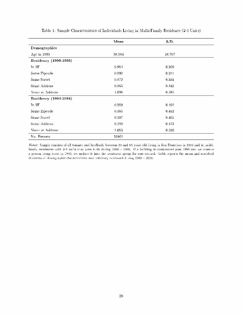
Table 1: Sample Characteristics of Individuals Living in Multi-Family Residence (2-4 Units)

Mean S.D.

Demographics

Age in 1993 38.584 10.707

Residency (1990-1993)

In SF 0.954 0.209

Same Zipcode 0.892 0.311

Same Street 0.872 0.334

Same Address 0.865 0.342

Years at Address 1.696 0.585

Residency (1994-2016)

In SF 0.589 0.492

Same Zipcode 0.365 0.482

Same Street 0.307 0.461

Same Address 0.289 0.453

Years at Address 1.653 0.599

No. Persons 55861

Notes: Sample consists of all tenants and landlords between 20 and 65 years old living in San Francisco in 1993 and in multi-

family residences with 2-4 units that were built during 1900 − 1990. If a building is constructed post 1993 and we observe

a person living there in 1993, we include it into the treatment group for rent control. Table reports the mean and standard

deviation of demographic characteristics and residency outcomes during 1990− 2016.

28

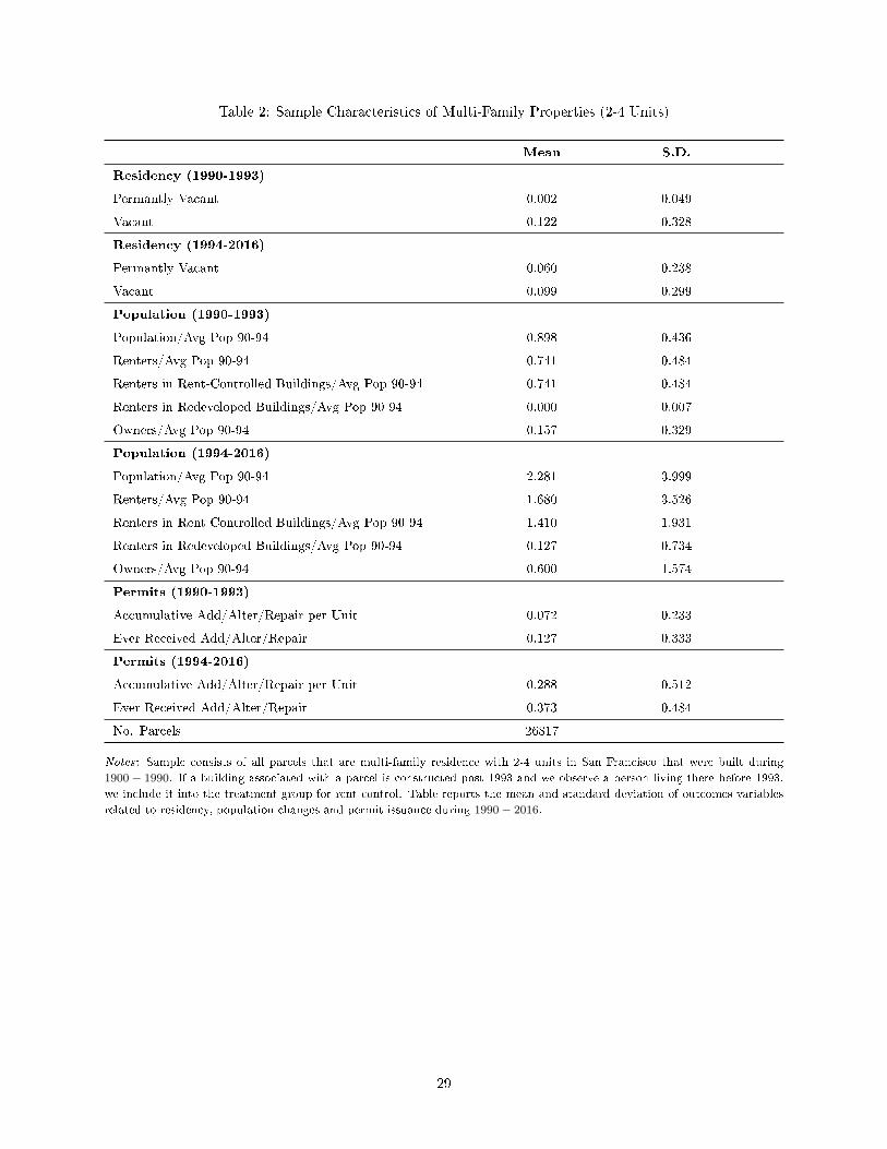
Table 2: Sample Characteristics of Multi-Family Properties (2-4 Units)

Mean S.D.

Residency (1990-1993)

Permantly Vacant 0.002 0.049

Vacant 0.122 0.328

Residency (1994-2016)

Permantly Vacant 0.060 0.238

Vacant 0.099 0.299

Population (1990-1993)

Population/Avg Pop 90-94 0.898 0.436

Renters/Avg Pop 90-94 0.741 0.484

Renters in Rent-Controlled Buildings/Avg Pop 90-94 0.741 0.484

Renters in Redeveloped Buildings/Avg Pop 90-94 0.000 0.007

Owners/Avg Pop 90-94 0.157 0.329

Population (1994-2016)

Population/Avg Pop 90-94 2.281 3.999

Renters/Avg Pop 90-94 1.680 3.526

Renters in Rent-Controlled Buildings/Avg Pop 90-94 1.410 1.931

Renters in Redeveloped Buildings/Avg Pop 90-94 0.127 0.734

Owners/Avg Pop 90-94 0.600 1.574

Permits (1990-1993)

Accumulative Add/Alter/Repair per Unit 0.072 0.233

Ever Received Add/Alter/Repair 0.127 0.333

Permits (1994-2016)

Accumulative Add/Alter/Repair per Unit 0.288 0.512

Ever Received Add/Alter/Repair 0.373 0.484

No. Parcels 26817

Notes: Sample consists of all parcels that are multi-family residence with 2-4 units in San Francisco that were built during

1900− 1990. If a building associated with a parcel is constructed post 1993 and we observe a person living there before 1993,

we include it into the treatment group for rent control. Table reports the mean and standard deviation of outcomes variables

related to residency, population changes and permit issuance during 1990− 2016.

29

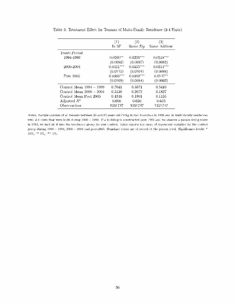
Table 3: Treatment E�ect for Tenants of Multi-Family Residence (2-4 Units)

(1) (2) (3)In SF Same Zip Same Address

Treat×Period1994-1999 0.0200∗∗ 0.0226∗∗∗ 0.0218∗∗∗

(0.0081) (0.0087) (0.0083)2000-2004 0.0451∗∗∗ 0.0355∗∗∗ 0.0354∗∗∗

(0.0115) (0.0104) (0.0088)Post 2005 0.0366∗∗∗ 0.0302∗∗∗ 0.0147∗∗

(0.0109) (0.0084) (0.0063)

Control Mean 1994− 1999 0.7641 0.5971 0.5410Control Mean 2000− 2004 0.5138 0.2672 0.1827Control Mean Post 2005 0.4346 0.1801 0.1135Adjusted R2 0.600 0.630 0.655Observations 1251747 1251747 1251747

Notes: Sample consists of all tenants between 20 and 65 years old living in San Francisco in 1993 and in multi-family residences

with 2-4 units that were built during 1900− 1990. If a building is constructed post 1993 and we observe a person living there

in 1993, we include it into the treatment group for rent control. Table reports the mean of dependent variables for the control

group during 1990− 1994, 2000− 2004 and post-2005. Standard errors are clustered at the person level. Signi�cance levels: *

10%, ** 5%, *** 1%.

30

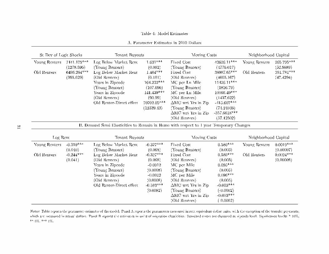
Table 4: Model Estimates

A. Parameter Estimates in 2010 Dollars

St Dev of Logit Shocks Tenant Buyouts Moving Costs Neighborhood Capital

Young Renters 7441.178*** Log Below Market Rent 1.631*** Fixed Cost 42626.11*** Young Renters 265.795***(1278.596) (Young Renters) (0.092) (Young Renters) (4776.017) (52.9889)

Old Renters 6496.264*** Log Below Market Rent 1.404*** Fixed Cost 38987.65*** Old Renters 291.781***(995.629) (Old Renters) (0.101) (Old Renters) (4005.167) (47.4294)

Years in Zipcode 164.222*** MC per Ln Mile 11426.11***(Young Renters) (107.696) (Young Renters) (1816.79)Years in Zipcode 141.439*** MC per Ln Mile 10066.49***(Old Renters) (90.99) (Old Renters) (1437.622)Old Renter-Direct e�ect 70702.05*** ∆MC wrt Yrs in Zip -415.607***

(12339.43) (Young Renters) (74.24046)∆MC wrt Yrs in Zip -357.6618***(Old Renters) (57.12502)

B. Demand Semi-Elasticities to Remain in Home with respect to 1 year Temporary Changes

Log Rent Tenant Buyouts Moving Costs Neighborhood Capital

Young Renters -0.210*** Log Below Market Rent -0.327*** Fixed Cost 0.580*** Young Renters 0.0019***(0.040) (Young Renters) (0.068) (Young Renters) (0.003) (0.00007)

Old Renters -0.244*** Log Below Market Rent -0.327*** Fixed Cost 0.580*** Old Renters 0.0024***(0.041) (Old Renters) (0.068) (Old Renters) (0.003) (0.00008)

Years in Zipcode -0.0012 MC per Mile 0.095***(Young Renters) (0.0008) (Young Renters) (0.005)Years in Zipcode -0.0012 MC per Mile 0.096***(Old Renters) (0.0008) (Old Renters) (0.005)Old Renter-Direct e�ect -0.583*** ∆MC wrt Yrs in Zip -0.003***

(0.0082) (Young Renters) (-0.0002)∆MC wrt Yrs in Zip -0.003***(Old Renters) (-0.0002)

Notes: Table reports the parameter estimates of the model. Panel A reports the parameters measured in rent equivalent dollar units, with the exception of the transfer payments,

which are measured in actual dollars. Panel B reports the estimates in units of migration elasticities. Standard errors are clustered at zipcode level. Signi�cance levels: * 10%,

** 5%, *** 1%.

31

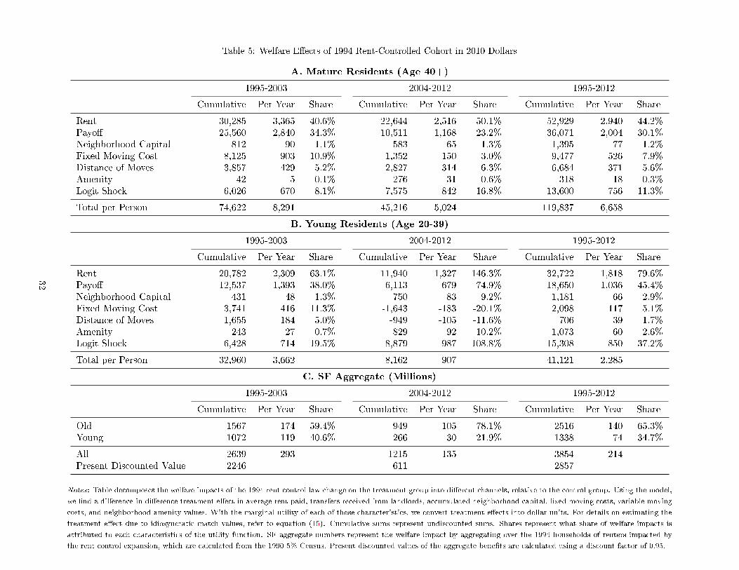
Table 5: Welfare E�ects of 1994 Rent-Controlled Cohort in 2010 Dollars

A. Mature Residents (Age 40+)

1995-2003 2004-2012 1995-2012

Cumulative Per Year Share Cumulative Per Year Share Cumulative Per Year Share

Rent 30,285 3,365 40.6% 22,644 2,516 50.1% 52,929 2,940 44.2%Payo� 25,560 2,840 34.3% 10,511 1,168 23.2% 36,071 2,004 30.1%Neighborhood Capital 812 90 1.1% 583 65 1.3% 1,395 77 1.2%Fixed Moving Cost 8,125 903 10.9% 1,352 150 3.0% 9,477 526 7.9%Distance of Moves 3,857 429 5.2% 2,827 314 6.3% 6,684 371 5.6%Amenity -42 -5 -0.1% -276 -31 -0.6% -318 -18 -0.3%Logit Shock 6,026 670 8.1% 7,575 842 16.8% 13,600 756 11.3%

Total per Person 74,622 8,291 45,216 5,024 119,837 6,658

B. Young Residents (Age 20-39)

1995-2003 2004-2012 1995-2012

Cumulative Per Year Share Cumulative Per Year Share Cumulative Per Year Share

Rent 20,782 2,309 63.1% 11,940 1,327 146.3% 32,722 1,818 79.6%Payo� 12,537 1,393 38.0% 6,113 679 74.9% 18,650 1,036 45.4%Neighborhood Capital 431 48 1.3% 750 83 9.2% 1,181 66 2.9%Fixed Moving Cost 3,741 416 11.3% -1,643 -183 -20.1% 2,098 117 5.1%Distance of Moves 1,655 184 5.0% -949 -105 -11.6% 706 39 1.7%Amenity 243 27 0.7% 829 92 10.2% 1,073 60 2.6%Logit Shock -6,428 -714 -19.5% -8,879 -987 -108.8% -15,308 -850 -37.2%

Total per Person 32,960 3,662 8,162 907 41,121 2,285

C. SF Aggregate (Millions)

1995-2003 2004-2012 1995-2012

Cumulative Per Year Share Cumulative Per Year Share Cumulative Per Year Share

Old 1567 174 59.4% 949 105 78.1% 2516 140 65.3%Young 1072 119 40.6% 266 30 21.9% 1338 74 34.7%

All 2639 293 1215 135 3854 214Present Discounted Value 2246 611 2857

Notes: Table decomposes the welfare impacts of the 1994 rent control law change on the treatment group into di�erent channels, relative to the control group. Using the model,

we �nd a di�erence-in-di�erence treatment e�ect in average rent paid, transfers received from landlords, accumulated neighborhood capital, �xed moving costs, variable moving

costs, and neighborhood amenity values. With the marginal utility of each of those characteristics, we convert treatment e�ects into dollar units. For details on estimating the

treatment e�ect due to idiosyncratic match values, refer to equation (15). Cumulative sums represent undiscounted sums. Shares represent what share of welfare impacts is

attributed to each characteristics of the utility function. SF aggregate numbers represent the welfare impact by aggregating over the 1994 households of renters impacted by

the rent control expansion, which are calculated from the 1990 5% Census. Present discounted values of the aggregate bene�ts are calculated using a discount factor of 0.95.

32

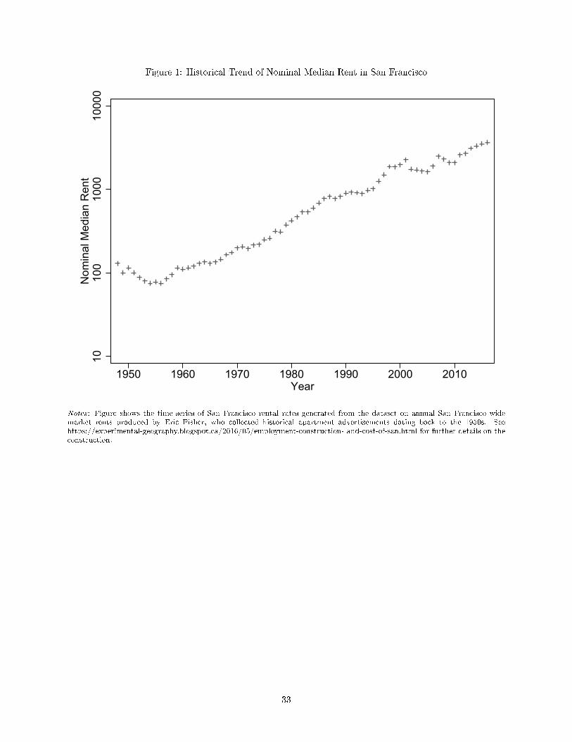
Figure 1: Historical Trend of Nominal Median Rent in San Francisco

1010

010

0010

000

Nom

inal

Med

ian

Ren

t

1950 1960 1970 1980 1990 2000 2010Year

Notes: Figure shows the time series of San Francisco rental rates generated from the dataset on annual San Francisco widemarket rents produced by Eric Fisher, who collected historical apartment advertisements dating back to the 1950s. Seehttps://experimental-geography.blogspot.ca/2016/05/employment-construction- and-cost-of-san.html for further details on theconstruction.

33

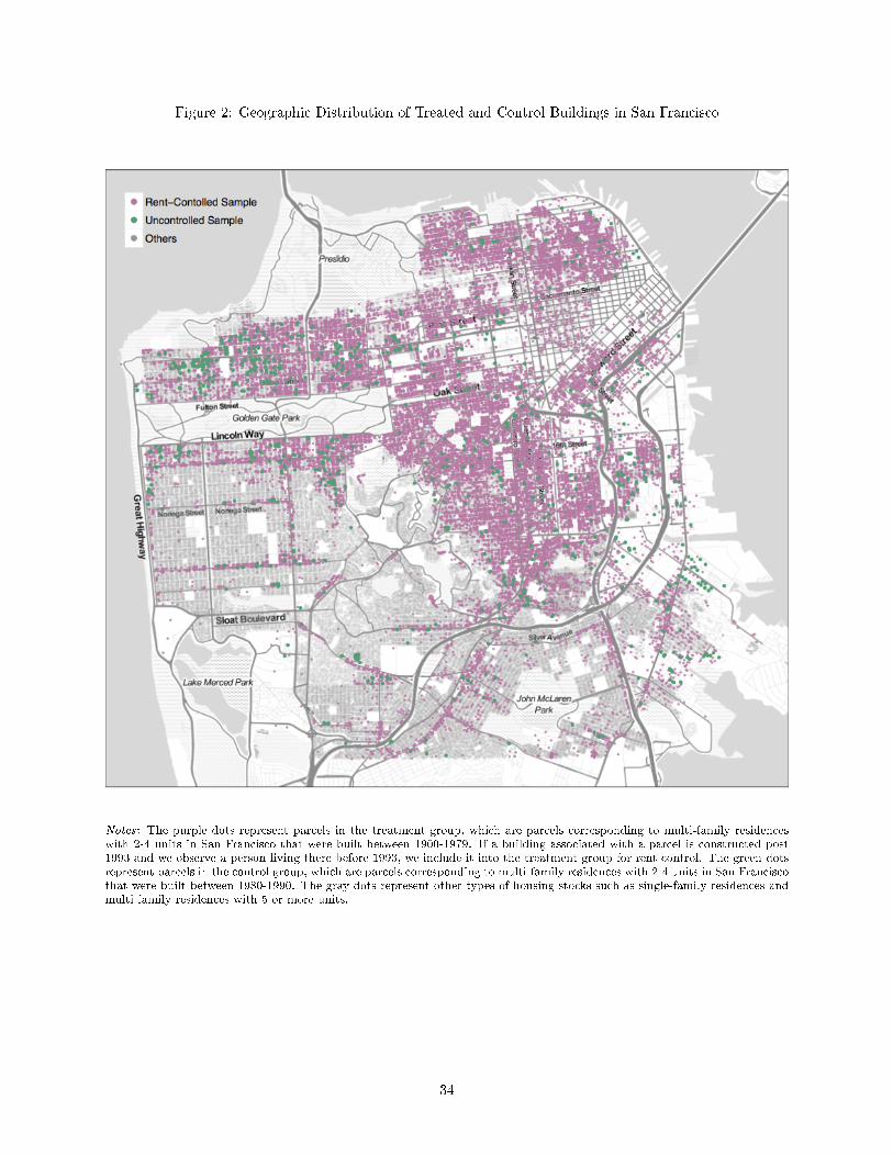
Figure 2: Geographic Distribution of Treated and Control Buildings in San Francisco

Notes: The purple dots represent parcels in the treatment group, which are parcels corresponding to multi-family residenceswith 2-4 units in San Francisco that were built between 1900-1979. If a building associated with a parcel is constructed post1993 and we observe a person living there before 1993, we include it into the treatment group for rent control. The green dotsrepresent parcels in the control group, which are parcels corresponding to multi-family residences with 2-4 units in San Franciscothat were built between 1980-1990. The gray dots represent other types of housing stocks such as single-family residences andmulti-family residences with 5 or more units.

34

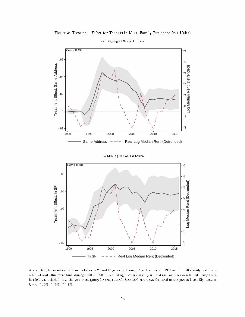
Figure 3: Treatment E�ect for Tenants in Multi-Family Residence (2-4 Units)

(a) Staying at Same Address

-.2

-.1

0.1

.2.3

.4.5

Log

Med

ian

Ren

t (D

etre

nded

)

-.02

0

.02

.04

.06T

reat

men

t Effe

ct: S

ame

Add

ress

1990 1995 2000 2005 2010 2015

Same Address Real Log Median Rent (Detrended)

Corr = 0.494

(b) Staying in San Francisco

-.2

-.1

0.1

.2.3

.4.5

Log

Med

ian

Ren

t (D

etre

nded

)

-.02

0

.02

.04

.06

Tre

atm

ent E

ffect

: In

SF

1990 1995 2000 2005 2010 2015

In SF Real Log Median Rent (Detrended)

Corr = 0.784

Notes: Sample consists of all tenants between 20 and 65 years old living in San Francisco in 1993 and in multi-family residences

with 2-4 units that were built during 1900− 1990. If a building is constructed post 1993 and we observe a tenant living there

in 1993, we include it into the treatment group for rent control. Standard errors are clustered at the person level. Signi�cance

levels: * 10%, ** 5%, *** 1%.

35

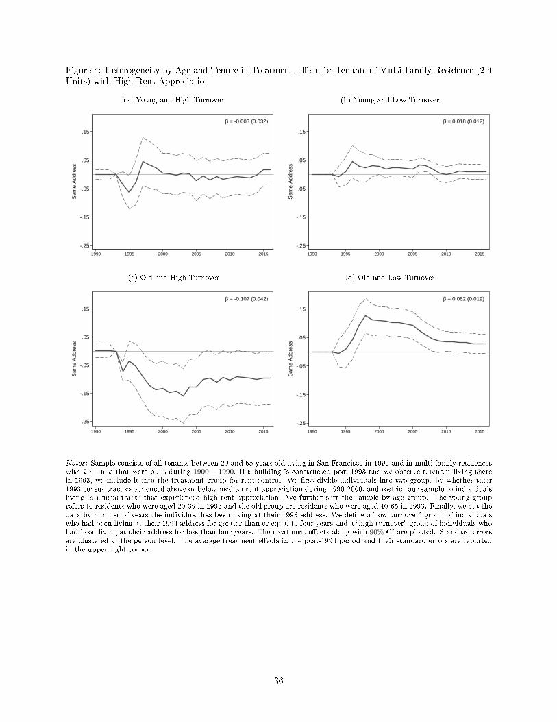
Figure 4: Heterogeneity by Age and Tenure in Treatment E�ect for Tenants of Multi-Family Residence (2-4Units) with High Rent Appreciation

(a) Young and High Turnover

-.25

-.15

-.05

.05

.15

Sam

e A

ddre

ss

1990 1995 2000 2005 2010 2015

β = -0.003 (0.032)

(b) Young and Low Turnover

-.25

-.15

-.05

.05

.15

Sam

e A

ddre

ss

1990 1995 2000 2005 2010 2015

β = 0.018 (0.012)

(c) Old and High Turnover

-.25

-.15

-.05

.05

.15

Sam

e A

ddre

ss

1990 1995 2000 2005 2010 2015

β = -0.107 (0.042)

(d) Old and Low Turnover

-.25

-.15

-.05

.05

.15

Sam

e A

ddre

ss

1990 1995 2000 2005 2010 2015

β = 0.062 (0.019)

Notes: Sample consists of all tenants between 20 and 65 years old living in San Francisco in 1993 and in multi-family residenceswith 2-4 units that were built during 1900− 1990. If a building is constructed post 1993 and we observe a tenant living therein 1993, we include it into the treatment group for rent control. We �rst divide individuals into two groups by whether their1993 census tract experienced above or below median rent appreciation during 1990-2000, and restrict our sample to individualsliving in census tracts that experienced high rent appreciation. We further sort the sample by age group. The young grouprefers to residents who were aged 20-39 in 1993 and the old group are residents who were aged 40-65 in 1993. Finally, we cut thedata by number of years the individual has been living at their 1993 address. We de�ne a �low turnover� group of individualswho had been living at their 1993 address for greater than or equal to four years and a �high turnover� group of individuals whohad been living at their address for less than four years. The treatment e�ects along with 90% CI are plotted. Standard errorsare clustered at the person level. The average treatment e�ects in the post-1994 period and their standard errors are reportedin the upper-right corner.

36

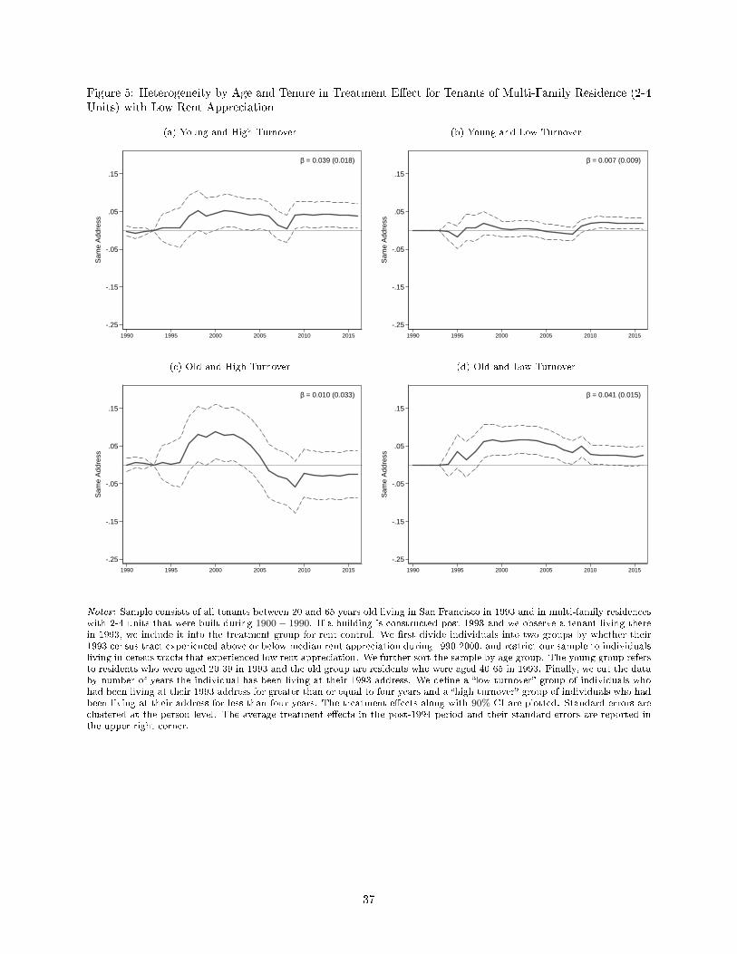
Figure 5: Heterogeneity by Age and Tenure in Treatment E�ect for Tenants of Multi-Family Residence (2-4Units) with Low Rent Appreciation

(a) Young and High Turnover

-.25

-.15

-.05

.05

.15

Sam

e A

ddre

ss

1990 1995 2000 2005 2010 2015

β = 0.039 (0.018)

(b) Young and Low Turnover

-.25

-.15

-.05

.05

.15

Sam

e A

ddre

ss

1990 1995 2000 2005 2010 2015

β = 0.007 (0.009)

(c) Old and High Turnover

-.25

-.15

-.05

.05

.15

Sam

e A

ddre

ss

1990 1995 2000 2005 2010 2015

β = 0.010 (0.033)

(d) Old and Low Turnover

-.25

-.15

-.05

.05

.15

Sam

e A

ddre

ss

1990 1995 2000 2005 2010 2015

β = 0.041 (0.015)

Notes: Sample consists of all tenants between 20 and 65 years old living in San Francisco in 1993 and in multi-family residenceswith 2-4 units that were built during 1900− 1990. If a building is constructed post 1993 and we observe a tenant living therein 1993, we include it into the treatment group for rent control. We �rst divide individuals into two groups by whether their1993 census tract experienced above or below median rent appreciation during 1990-2000, and restrict our sample to individualsliving in census tracts that experienced low rent appreciation. We further sort the sample by age group. The young group refersto residents who were aged 20-39 in 1993 and the old group are residents who were aged 40-65 in 1993. Finally, we cut the databy number of years the individual has been living at their 1993 address. We de�ne a �low turnover� group of individuals whohad been living at their 1993 address for greater than or equal to four years and a �high turnover� group of individuals who hadbeen living at their address for less than four years. The treatment e�ects along with 90% CI are plotted. Standard errors areclustered at the person level. The average treatment e�ects in the post-1994 period and their standard errors are reported inthe upper-right corner.

37

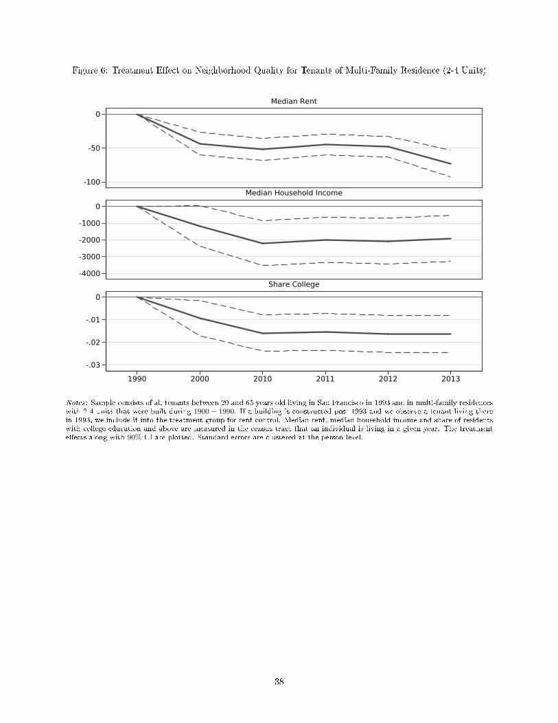
Figure 6: Treatment E�ect on Neighborhood Quality for Tenants of Multi-Family Residence (2-4 Units)

-100

-50

0

-4000

-3000

-2000

-1000

0

-.03

-.02

-.01

0

1990 2000 2010 2011 2012 2013

Median Rent

Median Household Income

Share College

Notes: Sample consists of all tenants between 20 and 65 years old living in San Francisco in 1993 and in multi-family residenceswith 2-4 units that were built during 1900− 1990. If a building is constructed post 1993 and we observe a tenant living therein 1993, we include it into the treatment group for rent control. Median rent, median household income and share of residentswith college education and above are measured in the census tract that an individual is living in a given year. The treatmente�ects along with 90% CI are plotted. Standard errors are clustered at the person level.

38

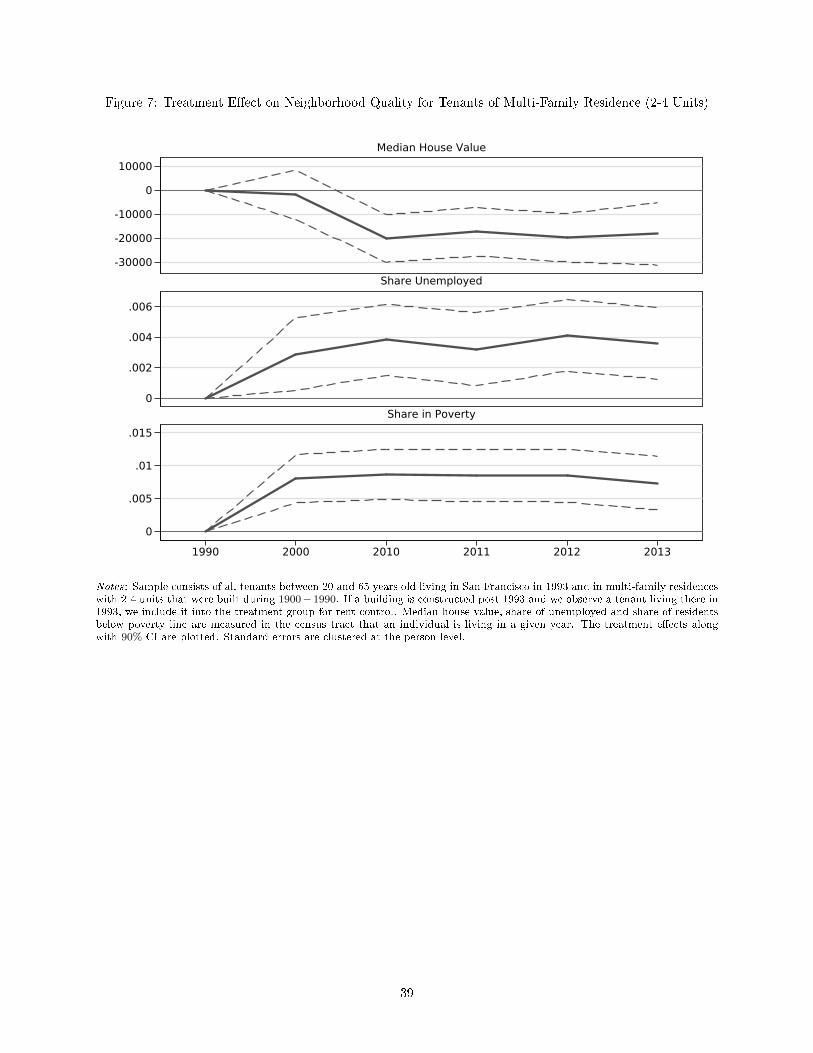
Figure 7: Treatment E�ect on Neighborhood Quality for Tenants of Multi-Family Residence (2-4 Units)

-30000

-20000

-10000

0

10000

0

.002

.004

.006

0

.005

.01

.015

1990 2000 2010 2011 2012 2013

Median House Value

Share Unemployed

Share in Poverty

Notes: Sample consists of all tenants between 20 and 65 years old living in San Francisco in 1993 and in multi-family residenceswith 2-4 units that were built during 1900− 1990. If a building is constructed post 1993 and we observe a tenant living there in1993, we include it into the treatment group for rent control. Median house value, share of unemployed and share of residentsbelow poverty line are measured in the census tract that an individual is living in a given year. The treatment e�ects alongwith 90% CI are plotted. Standard errors are clustered at the person level.

39

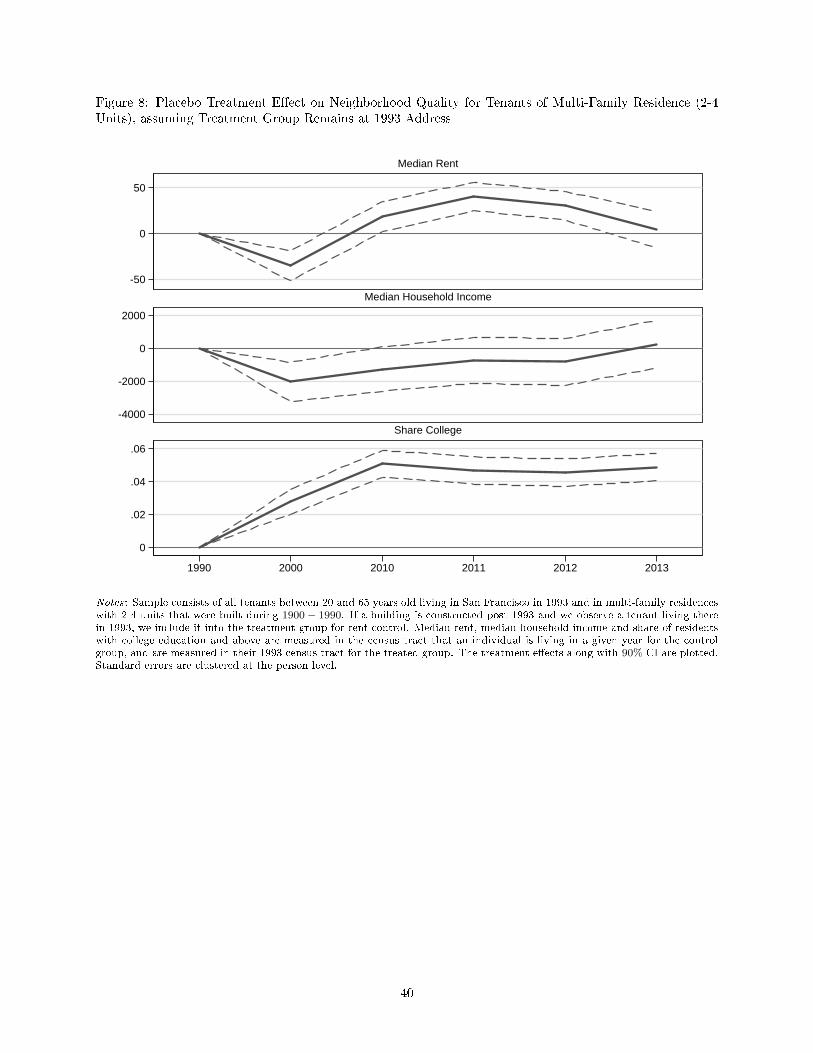
Figure 8: Placebo Treatment E�ect on Neighborhood Quality for Tenants of Multi-Family Residence (2-4Units), assuming Treatment Group Remains at 1993 Address

-50

0

50

-4000

-2000

0

2000

0

.02

.04

.06

1990 2000 2010 2011 2012 2013

Median Rent

Median Household Income

Share College

Notes: Sample consists of all tenants between 20 and 65 years old living in San Francisco in 1993 and in multi-family residenceswith 2-4 units that were built during 1900− 1990. If a building is constructed post 1993 and we observe a tenant living therein 1993, we include it into the treatment group for rent control. Median rent, median household income and share of residentswith college education and above are measured in the census tract that an individual is living in a given year for the controlgroup, and are measured in their 1993 census tract for the treated group. The treatment e�ects along with 90% CI are plotted.Standard errors are clustered at the person level.

40

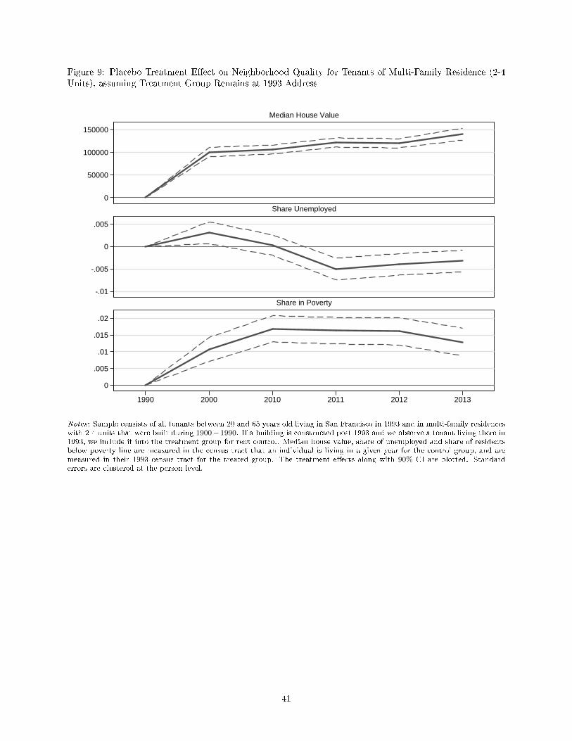
Figure 9: Placebo Treatment E�ect on Neighborhood Quality for Tenants of Multi-Family Residence (2-4Units), assuming Treatment Group Remains at 1993 Address

0

50000

100000

150000

-.01

-.005

0

.005

0

.005

.01

.015

.02

1990 2000 2010 2011 2012 2013

Median House Value

Share Unemployed

Share in Poverty

Notes: Sample consists of all tenants between 20 and 65 years old living in San Francisco in 1993 and in multi-family residenceswith 2-4 units that were built during 1900− 1990. If a building is constructed post 1993 and we observe a tenant living there in1993, we include it into the treatment group for rent control. Median house value, share of unemployed and share of residentsbelow poverty line are measured in the census tract that an individual is living in a given year for the control group, and aremeasured in their 1993 census tract for the treated group. The treatment e�ects along with 90% CI are plotted. Standarderrors are clustered at the person level.

41

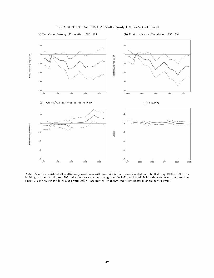
Figure 10: Treatment E�ect for Multi-Family Residence (2-4 Units)

(a) Population/Average Population 1990-1994

-.4

-.3

-.2

-.1

0

.1

Pop

ulat

ion/

Avg

Pop

90-

94

1990 1995 2000 2005 2010

(b) Renters/Average Population 1990-1994

-.4

-.3

-.2

-.1

0

.1

Ren

ters

/Avg

Pop

90-

94

1990 1995 2000 2005 2010

(c) Owners/Average Population 1990-1994

-.4

-.3

-.2

-.1

0

.1

Ow

ners

/Avg

Pop

90-

94

1990 1995 2000 2005 2010

(d) Vacancy

-.4

-.3

-.2

-.1

0

.1V

acan

t

1990 1995 2000 2005 2010 2015

Notes: Sample consists of all multi-family residences with 2-4 units in San Francisco that were built during 1900 − 1990. If abuilding is constructed post 1993 and we observe a tenant living there in 1993, we include it into the treatment group for rentcontrol. The treatment e�ects along with 90% CI are plotted. Standard errors are clustered at the parcel level.

42

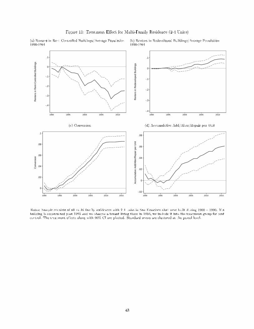
Figure 11: Treatment E�ect for Multi-Family Residence (2-4 Units)

(a) Renters in Rent-Controlled Buildings/Average Population1990-1994

-.4

-.3

-.2

-.1

0

.1

Ren

ters

in R

ent-

Con

trol

led

Bui

ldin

gs

1990 1995 2000 2005 2010

(b) Renters in Redeveloped Buildings/Average Population1990-1994

-.4

-.3

-.2

-.1

0

.1

Ren

ters

in R

edev

elop

ed B

uild

ings

1990 1995 2000 2005 2010

(c) Conversion

0

.02

.04

.06

.08

.1

Con

vers

ion

1990 1995 2000 2005 2010 2015

(d) Accumulative Add/Alter/Repair per Unit

-.02

0

.02

.04

.06

.08A

ccum

ulat

ive

Add

/Alte

r/R

epai

r pe

r U

nit

1990 1995 2000 2005 2010 2015

Notes: Sample consists of all multi-family residences with 2-4 units in San Francisco that were built during 1900 − 1990. If abuilding is constructed post 1993 and we observe a tenant living there in 1993, we include it into the treatment group for rentcontrol. The treatment e�ects along with 90% CI are plotted. Standard errors are clustered at the parcel level.

43

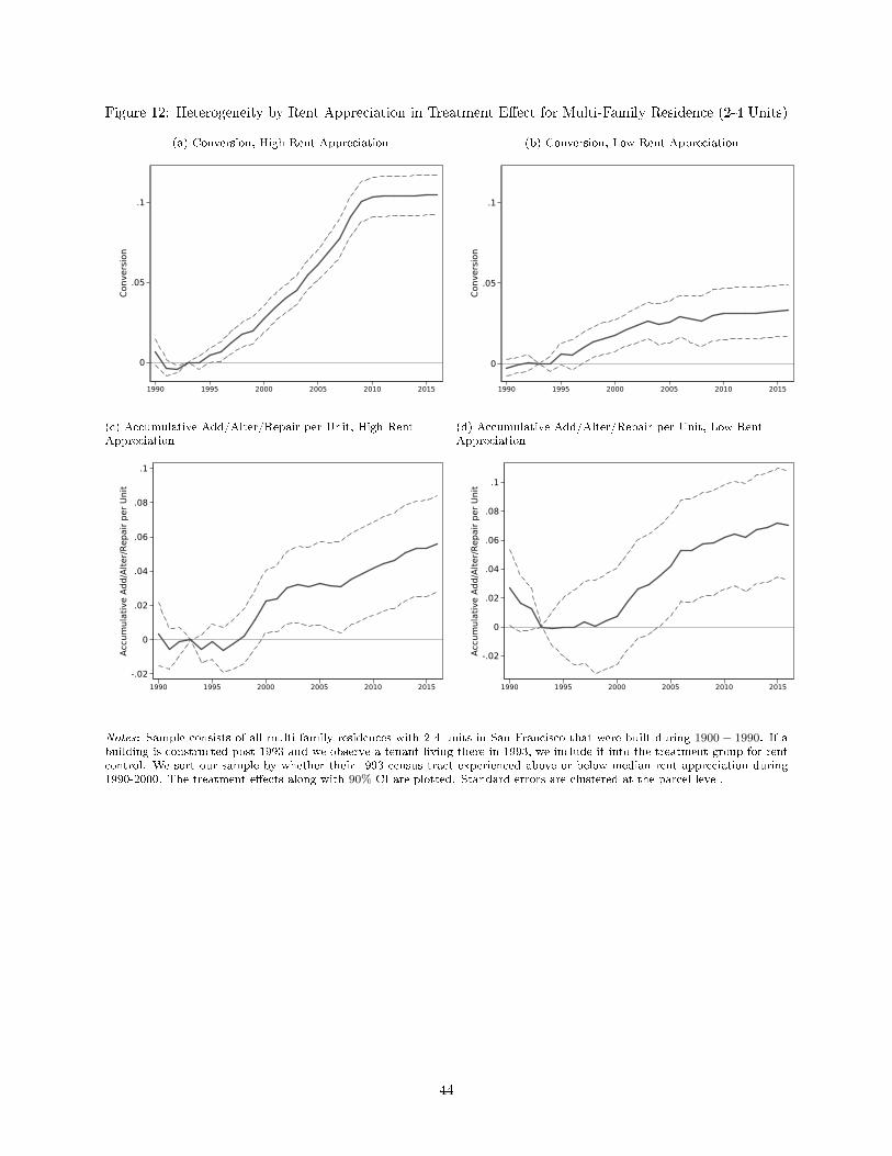
Figure 12: Heterogeneity by Rent Appreciation in Treatment E�ect for Multi-Family Residence (2-4 Units)

(a) Conversion, High Rent Appreciation

0

.05

.1

Conv

ersi

on

1990 1995 2000 2005 2010 2015

(b) Conversion, Low Rent Appreciation

0

.05

.1

Conv

ersi

on

1990 1995 2000 2005 2010 2015

(c) Accumulative Add/Alter/Repair per Unit, High RentAppreciation

-.02

0

.02

.04

.06

.08

.1

Accu

mul

ativ

e Ad

d/Al

ter/

Repa

ir pe

r Uni

t

1990 1995 2000 2005 2010 2015

(d) Accumulative Add/Alter/Repair per Unit, Low RentAppreciation

-.02

0

.02

.04

.06

.08

.1Ac

cum

ulat

ive

Add/

Alte

r/Re

pair

per U

nit

1990 1995 2000 2005 2010 2015

Notes: Sample consists of all multi-family residences with 2-4 units in San Francisco that were built during 1900 − 1990. If abuilding is constructed post 1993 and we observe a tenant living there in 1993, we include it into the treatment group for rentcontrol. We sort our sample by whether their 1993 census tract experienced above or below median rent appreciation during1990-2000. The treatment e�ects along with 90% CI are plotted. Standard errors are clustered at the parcel level.

44

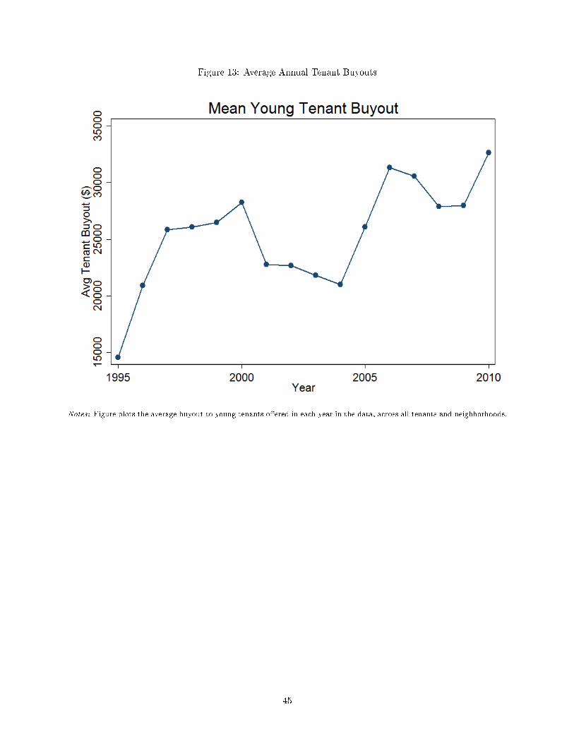
Figure 13: Average Annual Tenant Buyouts

Notes: Figure plots the average buyout to young tenants o�ered in each year in the data, across all tenants and neighborhoods.

45

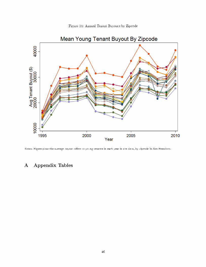
Figure 14: Annual Tenant Buyouts by Zipcode

Notes: Figure plots the average buyout o�ers to young tenants in each year in the data, by zipcode in San Francisco.

A Appendix Tables

46

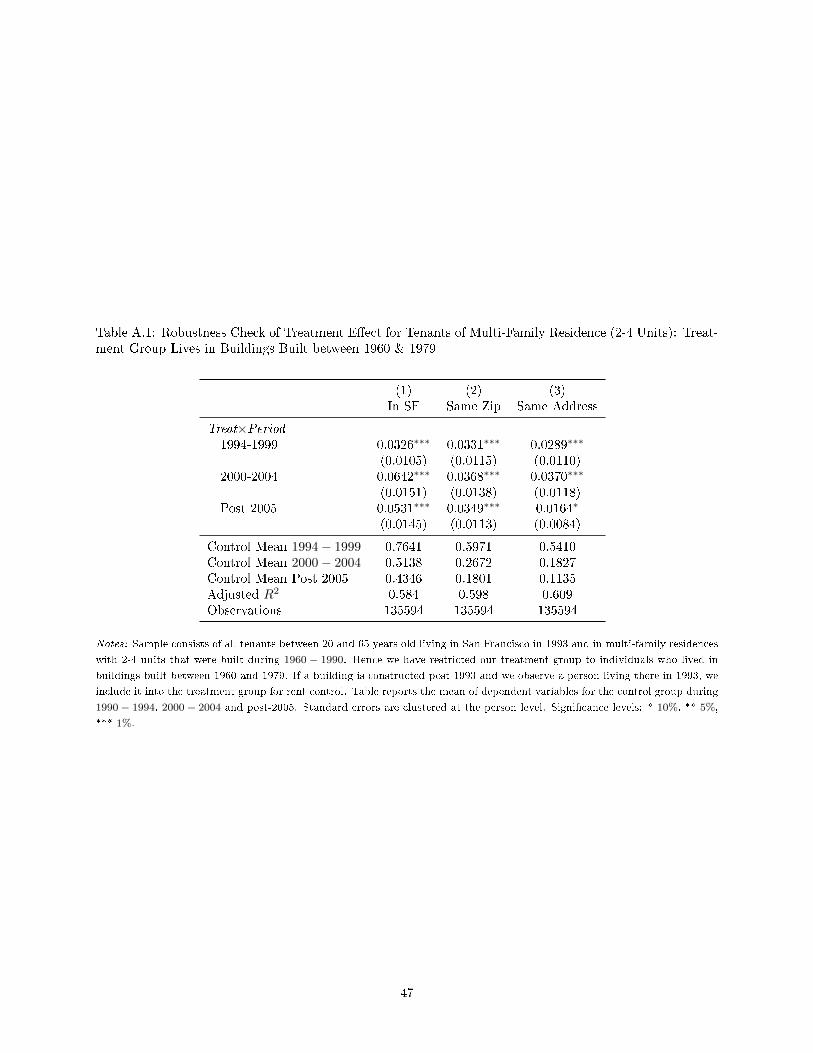
Table A.1: Robustness Check of Treatment E�ect for Tenants of Multi-Family Residence (2-4 Units): Treat-ment Group Lives in Buildings Built between 1960 & 1979

(1) (2) (3)In SF Same Zip Same Address

Treat×Period1994-1999 0.0326∗∗∗ 0.0331∗∗∗ 0.0289∗∗∗

(0.0105) (0.0115) (0.0110)2000-2004 0.0642∗∗∗ 0.0368∗∗∗ 0.0370∗∗∗

(0.0151) (0.0138) (0.0118)Post 2005 0.0531∗∗∗ 0.0349∗∗∗ 0.0164∗

(0.0145) (0.0113) (0.0084)

Control Mean 1994− 1999 0.7641 0.5971 0.5410Control Mean 2000− 2004 0.5138 0.2672 0.1827Control Mean Post 2005 0.4346 0.1801 0.1135Adjusted R2 0.584 0.598 0.609Observations 135594 135594 135594

Notes: Sample consists of all tenants between 20 and 65 years old living in San Francisco in 1993 and in multi-family residences

with 2-4 units that were built during 1960 − 1990. Hence we have restricted our treatment group to individuals who lived in

buildings built between 1960 and 1979. If a building is constructed post 1993 and we observe a person living there in 1993, we

include it into the treatment group for rent control. Table reports the mean of dependent variables for the control group during

1990− 1994, 2000− 2004 and post-2005. Standard errors are clustered at the person level. Signi�cance levels: * 10%, ** 5%,

*** 1%.

47

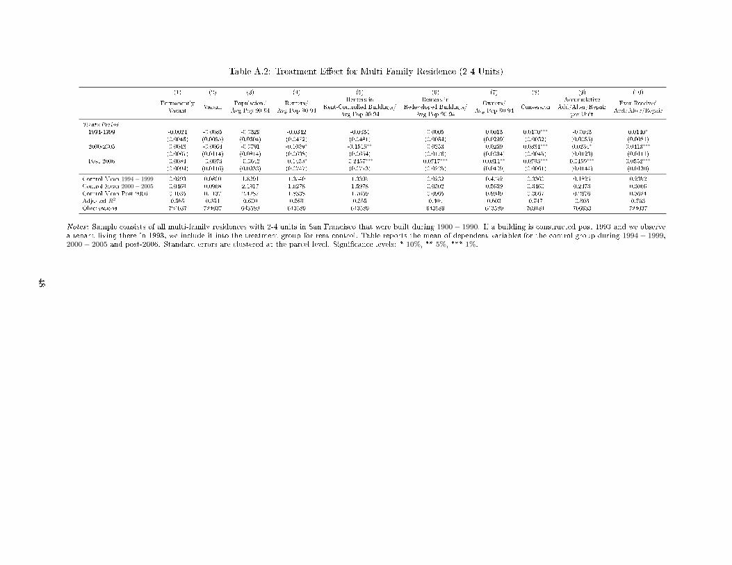
Table A.2: Treatment E�ect for Multi-Family Residence (2-4 Units)

(1) (2) (3) (4) (5) (6) (7) (8) (9) (10)

PermanentlyVacant

VacantPopulation/Avg Pop 90-94

Renters/Avg Pop 90-94

Renters inRent-Controlled Buildings/

Avg Pop 90-94

Renters inRedeveloped Buildings/

Avg Pop 90-94

Owners/Avg Pop 90-94

ConversionAccumulative

Add/Alter/Repairper Unit

Ever ReceivedAdd/Alter/Repair

Treat×Period1994-1999 -0.0024 -0.0085 -0.0329 -0.0342 -0.0434 0.0005 0.0013 0.0100∗∗∗ -0.0043 0.0140∗

(0.0046) (0.0095) (0.0604) (0.0472) (0.0481) (0.0084) (0.0299) (0.0032) (0.0085) (0.0081)2000-2005 0.0048 -0.0064 -0.0791 -0.1059∗ -0.1516∗∗ 0.0253 0.0269 0.0384∗∗∗ 0.0234∗ 0.0413∗∗∗

(0.0067) (0.0114) (0.0814) (0.0638) (0.0654) (0.0176) (0.0394) (0.0045) (0.0123) (0.0111)Post 2006 0.0084 -0.0076 -0.0642 -0.1453∗ -0.2457∗∗∗ 0.0717∗∗∗ 0.0811∗∗ 0.0793∗∗∗ 0.0459∗∗∗ 0.0552∗∗∗

(0.0094) (0.0116) (0.0933) (0.0747) (0.0773) (0.0225) (0.0409) (0.0061) (0.0144) (0.0130)

Control Mean 1994− 1999 0.0293 0.0800 1.8291 1.3540 1.3395 0.0232 0.4752 0.3360 0.1825 0.2352Control Mean 2000− 2005 0.0469 0.0968 2.1917 1.6278 1.5978 0.0502 0.5639 0.3460 0.2473 0.3066Control Mean Post 2006 0.1035 0.1137 2.4287 1.8338 1.7659 0.0965 0.5949 0.3667 0.2976 0.3624Adjusted R2 0.565 0.354 0.600 0.569 0.555 0.404 0.603 0.747 0.803 0.763Observations 724037 724037 643589 643589 643589 643589 643589 769181 706633 724037

Notes: Sample consists of all multi-family residences with 2-4 units in San Francisco that were built during 1900− 1990. If a building is constructed post 1993 and we observea tenant living there in 1993, we include it into the treatment group for rent control. Table reports the mean of dependent variables for the control group during 1994− 1999,2000− 2005 and post-2006. Standard errors are clustered at the parcel level. Signi�cance levels: * 10%, ** 5%, *** 1%.

48

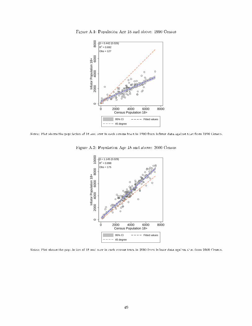
Figure A.1: Population Age 18 and above: 1990 Census

020

0040

0060

0080

00In

futo

r P

opul

atio

n 18

+

0 2000 4000 6000 8000Census Population 18+

95% CI Fitted values

45 degree

β = 0.442 (0.026)

R2 = 0.692

Obs = 127

Notes: Plot shows the population of 18 and over in each census tract in 1990 from Infutor data against that from 1990 Census.

Figure A.2: Population Age 18 and above: 2000 Census

020

0040

0060

0080

0010

000

Infu

tor

Pop

ulat

ion

18+

0 2000 4000 6000 8000Census Population 18+

95% CI Fitted values

45 degree

β = 1.145 (0.029)

R2 = 0.898

Obs = 175

Notes: Plot shows the population of 18 and over in each census tract in 2000 from Infutor data against that from 2000 Census.

49

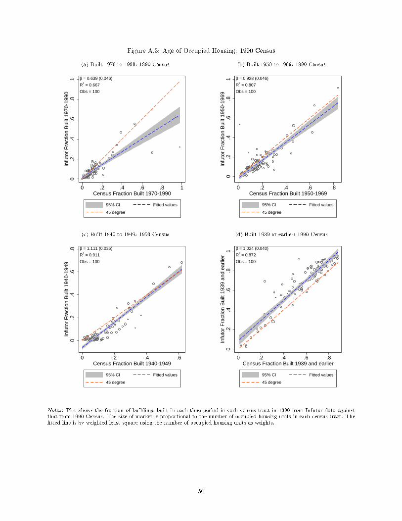
Figure A.3: Age of Occupied Housing: 1990 Census

(a) Built 1970 to 1990: 1990 Census

0.2

.4.6

.81

Infu

tor

Fra

ctio

n B

uilt

1970

-199

0

0 .2 .4 .6 .8 1Census Fraction Built 1970-1990

95% CI Fitted values

45 degree

β = 0.639 (0.046)

R2 = 0.667

Obs = 100

(b) Built 1950 to 1969: 1990 Census

0.2

.4.6

.81

Infu

tor

Fra

ctio

n B

uilt

1950

-196

9

0 .2 .4 .6 .8Census Fraction Built 1950-1969

95% CI Fitted values

45 degree

β = 0.928 (0.046)

R2 = 0.807

Obs = 100

(c) Built 1940 to 1949: 1990 Census

0.2

.4.6

.8In

futo

r F

ract

ion

Bui

lt 19

40-1

949

0 .2 .4 .6Census Fraction Built 1940-1949

95% CI Fitted values

45 degree

β = 1.111 (0.035)

R2 = 0.911

Obs = 100

(d) Built 1939 or earlier: 1990 Census0

.2.4

.6.8

1In

futo

r F

ract

ion

Bui

lt 19

39 a

nd e

arlie

r

0 .2 .4 .6 .8Census Fraction Built 1939 and earlier

95% CI Fitted values

45 degree

β = 1.024 (0.040)

R2 = 0.872

Obs = 100

Notes: Plot shows the fraction of buildings built in each time period in each census tract in 1990 from Infutor data againstthat from 1990 Census. The size of marker is proportional to the number of occupied housing units in each census tract. The�tted line is by weighted least square using the number of occupied housing units as weights.

50

Figure A.4: Age of Occupied Housing: 2000 Census

(a) Built 1980 to 2000: 2000 Census0

.2.4

.6.8

1In

futo

r F

ract

ion

Bui

lt 19

80-2

000

0 .2 .4 .6 .8Census Fraction Built 1980-2000

95% CI Fitted values

45 degree

β = 0.813 (0.024)

R2 = 0.876

Obs = 159

(b) Built 1960 to 1979: 2000 Census

0.2

.4.6

.81

Infu

tor

Fra

ctio

n B

uilt

1960

-197

9

0 .2 .4 .6 .8 1Census Fraction Built 1960-1979

95% CI Fitted values

45 degree

β = 1.083 (0.036)

R2 = 0.853

Obs = 159

(c) Built 1950 to 1959: 2000 Census

0.2

.4.6

.8In

futo

r F

ract

ion

Bui

lt 19

50-1

959

0 .2 .4 .6Census Fraction Built 1950-1959

95% CI Fitted values

45 degree

β = 0.955 (0.049)

R2 = 0.711

Obs = 159

(d) Built 1940 to 1949: 2000 Census

-.2

0.2

.4.6

.8In

futo

r F

ract

ion

Bui

lt 19

40-1

949

0 .2 .4 .6Census Fraction Built 1940-1949

95% CI Fitted values

45 degree

β = 1.323 (0.042)

R2 = 0.863

Obs = 159

(e) Built 1930 or earlier: 2000 Census

0.2

.4.6

.81

Infu

tor

Fra

ctio

n B

uilt

1939

and

ear

lier

0 .2 .4 .6 .8Census Fraction Built 1939 and earlier

95% CI Fitted values

45 degree

β = 1.144 (0.036)

R2 = 0.863

Obs = 159

Notes: Plot shows the fraction of buildings built in each time period in each census tract in 2000 from Infutor data againstthat from 2000 Census. The size of marker is proportional to the number of occupied housing units in each census tract. The�tted line is by weighted least square using the number of occupied housing units as weights.

51

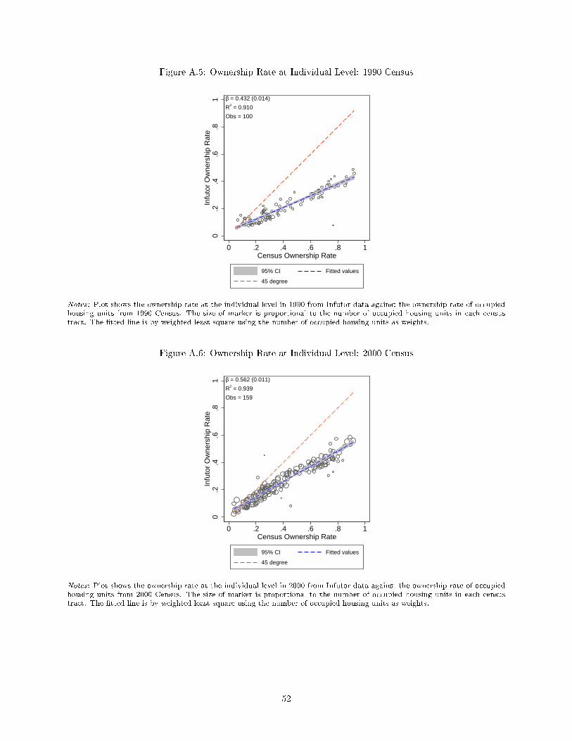
Figure A.5: Ownership Rate at Individual Level: 1990 Census

0.2

.4.6

.81

Infu

tor

Ow

ners

hip

Rat

e

0 .2 .4 .6 .8 1Census Ownership Rate

95% CI Fitted values

45 degree

β = 0.432 (0.014)

R2 = 0.910

Obs = 100

Notes: Plot shows the ownership rate at the individual level in 1990 from Infutor data against the ownership rate of occupiedhousing units from 1990 Census. The size of marker is proportional to the number of occupied housing units in each censustract. The �tted line is by weighted least square using the number of occupied housing units as weights.

Figure A.6: Ownership Rate at Individual Level: 2000 Census

0.2

.4.6

.81

Infu

tor

Ow

ners

hip

Rat

e

0 .2 .4 .6 .8 1Census Ownership Rate

95% CI Fitted values

45 degree

β = 0.562 (0.011)

R2 = 0.939

Obs = 159

Notes: Plot shows the ownership rate at the individual level in 2000 from Infutor data against the ownership rate of occupiedhousing units from 2000 Census. The size of marker is proportional to the number of occupied housing units in each censustract. The �tted line is by weighted least square using the number of occupied housing units as weights.

52