The Dirac Delta function -...
55
The Dirac Delta function Ernesto Est´ evez Rams [email protected] Instituto de Ciencia y Tecnolog´ ıa de Materiales (IMRE)-Facultad de F´ ısica Universidad de la Habana IUCr International School on Crystallography, Brazil, 2012. III Latinoamerican series
Transcript of The Dirac Delta function -...

The Dirac Delta function
Ernesto Estevez [email protected]
Instituto de Ciencia y Tecnologıa de Materiales (IMRE)-Facultad de FısicaUniversidad de la Habana
IUCr International School on Crystallography, Brazil, 2012.III Latinoamerican series
Introduction δ as a limit Properties Orthonormal Higher dimen. Recap Exercises Ref.
Outline
1 IntroductionDefining the Dirac Delta function
2 Dirac delta function as the limit of a family of functions
3 Properties of the Dirac delta function
4 Dirac delta function obtained from a complete set oforthonormal functions
Dirac comb
5 Dirac delta in higher dimensional space
6 Recapitulation
7 Exercises
8 References
2 / 45
The Dirac Delta function

Introduction δ as a limit Properties Orthonormal Higher dimen. Recap Exercises Ref.
The Kronecker Delta
Suppose we have a sequenceof values {a1, a2, . . .} and wewish to select algebraically aparticular value labeled by itsindex i
3 / 45
The Dirac Delta function

Introduction δ as a limit Properties Orthonormal Higher dimen. Recap Exercises Ref.
The Kronecker Delta
Definition (Kroneckerdelta)
Kδij =
{1 i = j0 i 6= j
Picking one member of a set algebraically
∑j=1
aKj δij = ai
4 / 45
The Dirac Delta function

Introduction δ as a limit Properties Orthonormal Higher dimen. Recap Exercises Ref.
The Kronecker Delta
Definition (Kroneckerdelta)
Kδij =
{1 i = j0 i 6= j
Picking one member of a set algebraically
∑j=1
aKj δij = ai
4 / 45
The Dirac Delta function

Introduction δ as a limit Properties Orthonormal Higher dimen. Recap Exercises Ref.
Properties of the Kronecker Delta
∑jKδij = 1: Normalization condition.
Kδij = Kδji: Symmetry property.
5 / 45
The Dirac Delta function
Introduction δ as a limit Properties Orthonormal Higher dimen. Recap Exercises Ref.
Properties of the Kronecker Delta
∑jKδij = 1: Normalization condition.
Kδij = Kδji: Symmetry property.
5 / 45
The Dirac Delta function

Introduction δ as a limit Properties Orthonormal Higher dimen. Recap Exercises Ref.
Spotting a point in the mountain profile
We want to pick upjust a narrow windowof the whole view
6 / 45
The Dirac Delta function

Introduction δ as a limit Properties Orthonormal Higher dimen. Recap Exercises Ref.
How to deal with continuous functions ?
We want to do thesame with acontinuous function.
7 / 45
The Dirac Delta function
Introduction δ as a limit Properties Orthonormal Higher dimen. Recap Exercises Ref.
Defining the Dirac Delta function
Consider a function f(x) continuous in the interval (a, b) and suppose wewant to pick up algebraically the value of f(x) at a particular point labeledby x0.In analogy with the Kronecker delta let us define a selector function Dδ(x)with the following two properties:∫ b
a f(x)Dδ(x− x0)dx = f(x0): Selector or sifting property
∫ baDδ(x− x0)dx = 1: Normalization condition
8 / 45
The Dirac Delta function
Introduction δ as a limit Properties Orthonormal Higher dimen. Recap Exercises Ref.
Defining the Dirac Delta function
To be more general consider f(x) to be continuous in the interval (a, b)except in a finite number of points where finite discontinuities occurs, thenthe Dirac Delta can be defined as
Definition (Dirac delta function)
∫ b
a
f(x)δ(x− x0)dx =
12[f(x−0 ) + f(x+
0 ] x0 ∈ (a, b)12f(x+
0 ) x0 = a12f(x−0 ) x0 = b
0 x0 /∈ (a, b)
9 / 45
The Dirac Delta function
Introduction δ as a limit Properties Orthonormal Higher dimen. Recap Exercises Ref.
A bit of history
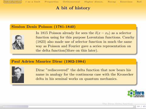
Simeon Denis Poisson (1781-1840)
In 1815 Poisson already for sees the δ(x− x0) as a selectorfunction using for this purpose Lorentzian functions. Cauchy(1823) also made use of selector function in much the sameway as Poisson and Fourier gave a series representation onthe delta function(More on this later).
Paul Adrien Maurice Dirac (1902-1984)
Dirac ”rediscovered” the delta function that now bears hisname in analogy for the continuous case with the Kroneckerdelta in his seminal works on quantum mechanics.
10 / 45
The Dirac Delta function

Introduction δ as a limit Properties Orthonormal Higher dimen. Recap Exercises Ref.
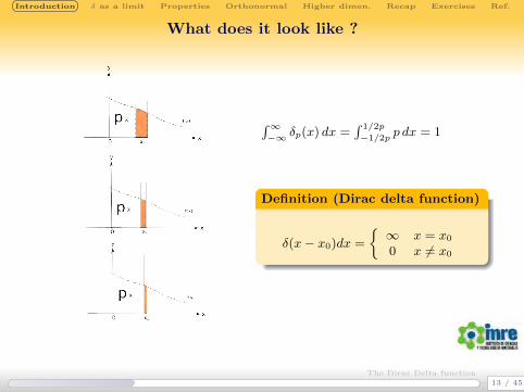
What does it look like ?
δp(x− x0) =
{p x ∈ (x0 − 1/2p, x0 + 1/2p)0 x /∈ (x0 − 1/2p, x0 + 1/2p)
11 / 45
The Dirac Delta function

Introduction δ as a limit Properties Orthonormal Higher dimen. Recap Exercises Ref.
What does it look like ?
p∫ x0+1/2p
x0−1/2pf(x)dx
12 / 45
The Dirac Delta function
Introduction δ as a limit Properties Orthonormal Higher dimen. Recap Exercises Ref.
What does it look like ?
∫∞−∞ δp(x) dx =
∫ 1/2p
−1/2pp dx = 1
Definition (Dirac delta function)
δ(x− x0)dx =
{∞ x = x0
0 x 6= x0
13 / 45
The Dirac Delta function

Introduction δ as a limit Properties Orthonormal Higher dimen. Recap Exercises Ref.
What does it look like ?
Definition (Dirac delta function)
δ(x− x0) =
{∞ x = x0
0 x 6= x0
The above expression is just ”formal”, the δ(x) must be always understood inthe context of its selector property i.e. within the integral
δ(x) is defined more rigorously in terms of a distribution or a functional(generalized function)
14 / 45
The Dirac Delta function

Introduction δ as a limit Properties Orthonormal Higher dimen. Recap Exercises Ref.
Dirac delta function as the limit of a family of functions
The Dirac delta function can be pictured as the limit in a sequence offunctions δp which must comply with two conditions:
lımp→∞∫∞−∞ δp(x)dx = 1: Normalization condition
lımp→∞δp(x6=0)
lımx→0 δp(x)= 0 Singularity condition.
15 / 45
The Dirac Delta function

Introduction δ as a limit Properties Orthonormal Higher dimen. Recap Exercises Ref.
... as the limit of Gaussian functions
δp(x) Gaussianfamily
δp(x) =
√p
πexp (−px2)
x
∆pHxL
�����
1
ã
&''''''''�����pΠ
"#############p �Π
1�"######p-1�"######p
16 / 45
The Dirac Delta function

Introduction δ as a limit Properties Orthonormal Higher dimen. Recap Exercises Ref.
... as the limit of Gaussian functions
Normalization condition
∫ ∞−∞
δp(x)dx =
√p
π
∫ ∞−∞
exp (−px2)dx =
√1
π
∫ ∞−∞
exp (−px2)d(√px) =√
1
π
∫ ∞−∞
exp (−t2)dt = 2
√1
π
∫ ∞0
exp (−t2)dt
I =∫∞
0e−t
2
dt
I2 =∫∞
0e−y
2
dy∫∞
0e−z
2
dz =∫ ∫∞
0exp (y2 + z2)dydz
17 / 45
The Dirac Delta function

Introduction δ as a limit Properties Orthonormal Higher dimen. Recap Exercises Ref.
Normalization condition
r2 = y2 + z2
y = r cosφz = r sinφ
I2 =
∫ π/20
dφ∫∞
0e−r
2
rdr = π4
∫∞0e−sds = π
4
I =√π
2∫∞−∞ δp(x)dx = 1
18 / 45
The Dirac Delta function

Introduction δ as a limit Properties Orthonormal Higher dimen. Recap Exercises Ref.
... as the limit of Gaussian functions
Singularity condition
lımp→∞
δp(x 6= 0)
lımx→0 δp(x)=
lımp→∞
√pπe−px
2√pπ
= 0
19 / 45
The Dirac Delta function

Introduction δ as a limit Properties Orthonormal Higher dimen. Recap Exercises Ref.
... as the limit of Lorentzian functions
δp(x) Lorentzianfamily
δp(x) =1
p
p
1 + p2x2
x
∆pHxL
�����������
p
2 Π
�����
p
Π
1�p-1�p
20 / 45
The Dirac Delta function

Introduction δ as a limit Properties Orthonormal Higher dimen. Recap Exercises Ref.
... as the limit of Lorentzian functions
Normalization condition
∫ ∞−∞
δp(x)dx =1
π
∫ ∞−∞
pdx
1 + p2x2=
1
π
∫ ∞−∞
dt
1 + t2=
1
πlımk→∞
arctan t|t=kt=−k =2
πlımk→∞
arctan k = 1
x
y
Π�2
ArcTanHxL
21 / 45
The Dirac Delta function

Introduction δ as a limit Properties Orthonormal Higher dimen. Recap Exercises Ref.
... as the limit of Lorentzian functions
Singularity condition
lımp→∞
δp(x 6= 0)
lımx→0 δp(x)=
1
πlımp→∞
p1+p2x2
p=
1
πlımp→∞
1
1 + p2x2= 0
22 / 45
The Dirac Delta function

Introduction δ as a limit Properties Orthonormal Higher dimen. Recap Exercises Ref.
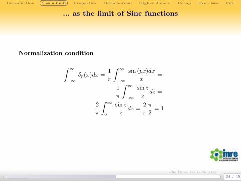
... as the limit of Sinc functions
δp(x) Sinc family
δp(x) =p
π
sin px
pxx
∆pHxL
�����
p
Π
�����
Π
p
2 �����
Π
p
3 �����
Π
p
23 / 45
The Dirac Delta function
Introduction δ as a limit Properties Orthonormal Higher dimen. Recap Exercises Ref.
... as the limit of Sinc functions
Normalization condition
∫ ∞−∞
δp(x)dx =1
π
∫ ∞−∞
sin (px)dx
x=
1
π
∫ ∞−∞
sin z
zdz =
2
π
∫ ∞0
sin z
zdz =
2
π
π
2= 1
24 / 45
The Dirac Delta function
Introduction δ as a limit Properties Orthonormal Higher dimen. Recap Exercises Ref.
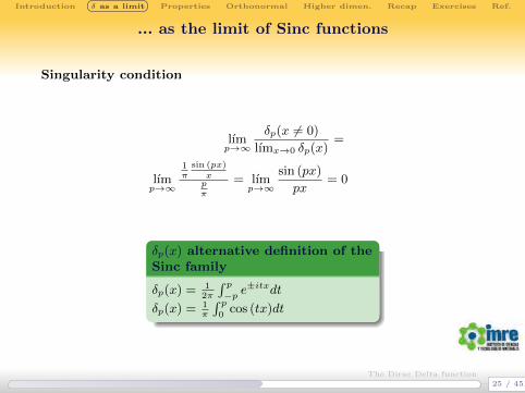
... as the limit of Sinc functions
Singularity condition
lımp→∞
δp(x 6= 0)
lımx→0 δp(x)=
lımp→∞
1π
sin (px)xpπ
= lımp→∞
sin (px)
px= 0
δp(x) alternative definition of theSinc family
δp(x) = 12π
∫ p−p e
±itxdt
δp(x) = 1π
∫ p0
cos (tx)dt
25 / 45
The Dirac Delta function
Introduction δ as a limit Properties Orthonormal Higher dimen. Recap Exercises Ref.
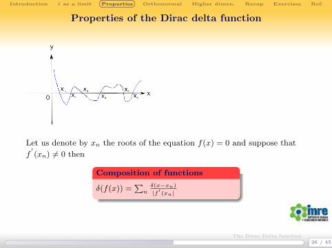
Properties of the Dirac delta function
Let us denote by xn the roots of the equation f(x) = 0 and suppose that
f′(xn) 6= 0 then
Composition of functions
δ(f(x)) =∑nδ(x−xn)
|f ′ (xn|
26 / 45
The Dirac Delta function

Introduction δ as a limit Properties Orthonormal Higher dimen. Recap Exercises Ref.
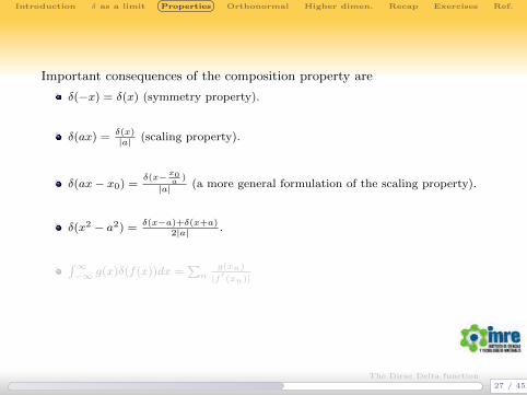
Important consequences of the composition property are
δ(−x) = δ(x) (symmetry property).
δ(ax) =δ(x)|a| (scaling property).
δ(ax− x0) =δ(x− x0
a)
|a| (a more general formulation of the scaling property).
δ(x2 − a2) =δ(x−a)+δ(x+a)
2|a| .
∫∞−∞ g(x)δ(f(x))dx =
∑n
g(xn)
|f ′ (xn)|
27 / 45
The Dirac Delta function

Introduction δ as a limit Properties Orthonormal Higher dimen. Recap Exercises Ref.
Important consequences of the composition property are
δ(−x) = δ(x) (symmetry property).
δ(ax) =δ(x)|a| (scaling property).
δ(ax− x0) =δ(x− x0
a)
|a| (a more general formulation of the scaling property).
δ(x2 − a2) =δ(x−a)+δ(x+a)
2|a| .
∫∞−∞ g(x)δ(f(x))dx =
∑n
g(xn)
|f ′ (xn)|
27 / 45
The Dirac Delta function

Introduction δ as a limit Properties Orthonormal Higher dimen. Recap Exercises Ref.
Convolution
Convolution
f(x)⊗δ(x+x0) =∫∞−∞ f(ς)δ(ς−(x+x0))dς = f(x+x0)
The effect of convolving with the position-shifted Dirac delta is to shift f(t)by the same amount.
∫∞−∞ δ(ζ − x)δ(x− η)dx = δ(ζ − η))
28 / 45
The Dirac Delta function

Introduction δ as a limit Properties Orthonormal Higher dimen. Recap Exercises Ref.
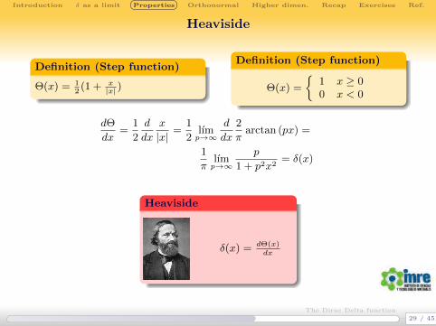
Heaviside
Definition (Step function)
Θ(x) = 12(1 + x
|x| )
Definition (Step function)
Θ(x) =
{1 x ≥ 00 x < 0
dΘ
dx=
1
2
d
dx
x
|x| =1
2lımp→∞
d
dx
2
πarctan (px) =
1
πlımp→∞
p
1 + p2x2= δ(x)
Heaviside
δ(x) = dΘ(x)dx
29 / 45
The Dirac Delta function
Introduction δ as a limit Properties Orthonormal Higher dimen. Recap Exercises Ref.
Heaviside
Definition (Step function)
Θ(x) = 12(1 + x
|x| )
Definition (Step function)
Θ(x) =
{1 x ≥ 00 x < 0
dΘ
dx=
1
2
d
dx
x
|x| =1
2lımp→∞
d
dx
2
πarctan (px) =
1
πlımp→∞
p
1 + p2x2= δ(x)
Heaviside
δ(x) = dΘ(x)dx
29 / 45
The Dirac Delta function

Introduction δ as a limit Properties Orthonormal Higher dimen. Recap Exercises Ref.
Heaviside
x
y
p=0.5
x
y
p=2
x
y
p=1
x
y
p=5
30 / 45
The Dirac Delta function

Introduction δ as a limit Properties Orthonormal Higher dimen. Recap Exercises Ref.
Fourier transform of the Dirac delta function
Fourier transform
Γ [δ(x)] = δ(x∗) ≡∫∞−∞ δ(x) exp (−2πix∗x)dx = 1
This property allow us to state yet another definition of the Dirac delta asthe inverse Fourier transform of f(x) = 1
Definition (Dirac delta function)
δ(x) =
∫ ∞−∞
exp (2πix∗x)dx∗
31 / 45
The Dirac Delta function

Introduction δ as a limit Properties Orthonormal Higher dimen. Recap Exercises Ref.
Dirac delta function obtained from a complete set oforthonormal functions
Let the set of functions {ψn} be a complete system of orthonormal functionsin the interval (a, b) and let x and x0 be inner points of that interval. Then
Theorem (Orthonormal functions)∑n ψ∗n(x)ψn(x0) = δ(x− x0)
To proof the theorem we shall demonstrate that the left hand side has thesifting property of the Dirac distribution
I =∫ baf(x)
∑n ψ∗n(x)ψn(x0)dx = f(x0)
f(x) =∑m cmψm(x) cm =
∫ baf(x)ψ∗m(x)dx
32 / 45
The Dirac Delta function

Introduction δ as a limit Properties Orthonormal Higher dimen. Recap Exercises Ref.
Dirac delta function obtained from a complete set oforthonormal functions
I =
∫ b
a
∑m
cmψm(x)∑n
ψ∗n(x)ψn(x0)dx =
∑m
cm∑n
ψn(x0)
∫ b
a
ψ∗n(x)ψm(x)dx
∫ baψ∗n(x)ψm(x)dx = Kδmn
I =∑n
cm∑n
ψn(x0)Kδmn =∑n
cmψm(x0) = f(x0)
33 / 45
The Dirac Delta function

Introduction δ as a limit Properties Orthonormal Higher dimen. Recap Exercises Ref.
Dirac comb
Definition (Dirac comb)∑∞m=−∞ δ(x−ma)
34 / 45
The Dirac Delta function

Introduction δ as a limit Properties Orthonormal Higher dimen. Recap Exercises Ref.
Dirac comb
The set { 1√(|a|)
exp (2πinx/a)} forms a complete set of orthonormal
functions, then
δ(x) = 1|a|∑∞n=−∞ exp (2πinx/a)
each summand in the LHS in the above expression is periodic with period|a| therefore the whole sum is periodic with the same period and
Dirac comb∑∞m=−∞ δ(x−ma) = 1
|a|∑∞n=−∞ exp (2πinx/a)
35 / 45
The Dirac Delta function

Introduction δ as a limit Properties Orthonormal Higher dimen. Recap Exercises Ref.
Fourier transform of a Dirac comb
∫ ∞−∞
∞∑m=−∞
δ(x−ma) exp(−2πix∗x)dx =
∞∑m=−∞
∫ ∞−∞
δ(x−ma) exp(−2πix∗x)dx =
∞∑m=−∞
exp(2πix∗ma)
Theorem (Fourier transform of a Dirac comb)
Γ [∑∞m=−∞ δ(x−ma)] = 1
|a|∑∞h=−∞ δ(x
∗ − h/a) = |a∗|∑∞h=−∞ δ(x
∗ − ha∗)
The Fourier transform of a Dirac comb is a Dirac comb
36 / 45
The Dirac Delta function

Introduction δ as a limit Properties Orthonormal Higher dimen. Recap Exercises Ref.
Dirac delta in higher dimensional space
Dirac delta in higher dimensions. Cartesian coordinates∫· ··∫f(~x)δ(~x− ~x0)dNx = f( ~x0)
which comes from∫· ··∫f(x1, x1, . . . xN )δ(x1−x01)δ(x2−x02) . . . δ(xN−x0N )dx1dx2 . . . dxN =
f( ~x01, x02, . . . x0N )
Definition (Dirac delta in higher dimensions. Cartesiancoordinates)
δ(~x− ~x0) = δ(x1 − x01)δ(x2 − x02) . . . δ(xN − x0N ) =∏Ns=1 δ(xs − x0s)
37 / 45
The Dirac Delta function

Introduction δ as a limit Properties Orthonormal Higher dimen. Recap Exercises Ref.
General coordinates
{xi}: Cartesian coordinates{yi}: General coordinates
x1 = x1(y1, . . . yN )
x2 = x2(y1, . . . yN )
. . .
xN = xN (y1, . . . yN )
J(y1, y2, . . . , yN ) =
∣∣∣∣∣∣∣∣∣∂x1∂y1
∂x1∂y2
. . . ∂x1∂yN
∂x2∂y1
∂x2∂y2
. . . ∂x2∂yN
. . . . . . . . . . . .∂xN∂y1
∂xN∂y2
. . . ∂xN∂yN
∣∣∣∣∣∣∣∣∣Definition (Dirac delta in higherdimensions. General coordinates)
δ(~x− ~x0) = 1|J(y1,y2,...,yN )|δ(~y − ~y0)
38 / 45
The Dirac Delta function

Introduction δ as a limit Properties Orthonormal Higher dimen. Recap Exercises Ref.
Oblique coordinates
x1 = a11y1 + a12y2 . . . a1NyNx2 = a11y1 + a22y2 . . . a2NyN
...xN = aN1y1 + aN2y2 . . . aNNyN
J(y1, y2, . . . , yN ) =∣∣∣∣∣∣∣∣a11 a12 . . . a1N
a21 a22 . . . a2N
. . . . . . . . . . . .aN1 aN2 . . . aNN
∣∣∣∣∣∣∣∣
~x =
a11 a12 . . . a1N
a21 a22 . . . a2N
. . . . . . . . . . . .aN1 aN2 . . . aNN
~y
Definition (Dirac delta in higherdimensions. Oblique coordinates)
δ(~x− ~x0) = 1| ||A|| |δ(~y− ~y0) = 1√
| ||G|| |δ(~y− ~y0)
39 / 45
The Dirac Delta function

Introduction δ as a limit Properties Orthonormal Higher dimen. Recap Exercises Ref.
Recap: Definitions
δ(x− x0)dx =
{∞ x = x0
0 x 6= x0
δ(x) =d
dx
(1
2(1 +
x
|x| ))
δ(x) = lımp→∞
√p
πexp (−px2)
δ(x) = lımp→∞
1
p
p
1 + p2x2
δ(x) = lımp→∞
p
π
sin px
px
δ(x) =
∫ ∞−∞
exp (2πix∗x)dx∗
δ(x− x0) =∑n
ψ∗n(x)ψn(x0)
where {ψ∗n(x)} is a complete set of orthornormal functions.
40 / 45
The Dirac Delta function

Introduction δ as a limit Properties Orthonormal Higher dimen. Recap Exercises Ref.
Recap: Properties
∫ b
a
f(x)δ(x− x0)dx =
12[f(x−0 ) + f(x+
0 ] x0 ∈ (a, b)12f(x+
0 ) x0 = a12f(x−0 ) x0 = b
0 x0 /∈ (a, b)
δ(f(x)) =∑n
δ(x− xn)
|f ′(xn|
∫ ∞−∞
g(x)δ(f(x))dx =∑n
g(xn)
|f ′(xn)|
δ(−x) = δ(x) δ(ax− x0) =δ(x− x0
a)
|a|
δ(x2 − a2) =δ(x− a) + δ(x+ a)
2|a| f(x)⊗ δ(x+ x0) = f(x+ x0)
Γ [
∞∑m=−∞
δ(x−ma)] = |a∗|∞∑
h=−∞
δ(x∗ − ha∗) Γ [δ(x)] = δ(x∗) = 1
∞∑m=−∞
δ(x−ma) =1
|a|
∞∑n=−∞
exp (2πinx/a)
41 / 45
The Dirac Delta function

Introduction δ as a limit Properties Orthonormal Higher dimen. Recap Exercises Ref.
Recap: Higher Dimensions
Cartesian coordinates:∫· · ·∫f(~x)δ(~x− ~x0)dNx = f( ~x0)
δ(~x− ~x0) = δ(x1 − x01)δ(x2 − x02) . . . δ(xN − x0N ) =
N∏s=1
δ(xs − x0s)
General Coordinates {yi}:
δ(~x− ~x0) =1
|J(y1, y2, . . . , yN )|δ(~y − ~y0)
Oblique Coordinates ~x = A · ~y:
δ(~x− ~x0) =1
| ||A|| |δ(~y − ~y0) =1√| ||G|| |
δ(~y − ~y0)
42 / 45
The Dirac Delta function

Introduction δ as a limit Properties Orthonormal Higher dimen. Recap Exercises Ref.
Exercises
Prove:
δ(f(x)) =∑nδ(x−xn)
|f ′ (xn|(Hint: develop f(x) in Taylor series around xn and
prove the sifting property with δ(f(x)))
∑∞n=−∞ f(na) = |x∗|
∑∞m=−∞ f(mx∗) (Poisson summation formula)
lımp→∞sin ((2p+1)π
x−x0a
)
sin (π x−x0a
)= |a|
∑∞m=−∞ δ(x− x0 −ma)
43 / 45
The Dirac Delta function

Introduction δ as a limit Properties Orthonormal Higher dimen. Recap Exercises Ref.
Exercises
Prove that on the limit p→∞ the sawtooth funtion tends to the Diraccomb
44 / 45
The Dirac Delta function
Introduction δ as a limit Properties Orthonormal Higher dimen. Recap Exercises Ref.
References
Prof. RNDr. Jiri Komrska.The Dirac distributionhttp://physics.fme.vutbr.cz/∼komrska
V. BalakrishnanAll about the Dirac Delta Function(?)
45 / 45
The Dirac Delta function
![Blockpraktikum [0.7ex] zur Statistik mit R f3](https://static.fdocument.pub/doc/165x107/5c92917209d3f26a458c925f/blockpraktikum-07ex-zur-statistik-mit-r-gt-f3-.jpg)