
THE BLACK-SCHOLES-MERTON MODEL 指導老師:王詩韻老師 學生:曾雅琪 (69936017)...
57
THE BLACK-SCHOLES-MERTON THE BLACK-SCHOLES-MERTON MODEL MODEL 指指指指 指指指指指 : 指指 指指指 : (69936017) 指指指 , (69936011)
-
Upload
malcolm-butler -
Category
Documents
-
view
313 -
download
0
Transcript of THE BLACK-SCHOLES-MERTON MODEL 指導老師:王詩韻老師 學生:曾雅琪 (69936017)...

THE BLACK-SCHOLES-MERTON THE BLACK-SCHOLES-MERTON MODELMODEL
指導老師:王詩韻老師學生:曾雅琪 (69936017),藍婉綺 (69936011)

Contents
Lognormal property of stock prices The distribution of the rate of return The expected return Volatility Concept underlying the Black-Scholes-Merton differential
equation Derivation of the Black-Scholes-Merton differential equation Risk-neutral valuation Black-Scholes pricing formulas Cumulative normal distribution function Implied volatilities Dividends
Assume
S
S
S
S
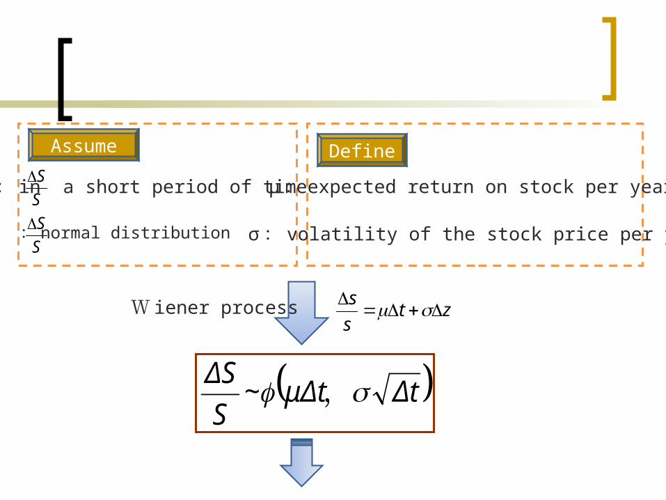
: in a short period of time(Δt)
: normal distribution
Define
μ: expected return on stock per year
σ: volatility of the stock price per year
W iener process zts
s
ΔtμΔt,~S
ΔS

TT
S
SSS T
T ,2
~lnlnln2
00
TTSST ,
2ln~ln
2
0
ΔtμΔt,~S
ΔS
dztxbdttxadx ),(),( dzSS
GdtS
S
G
t
GS
S
GdG
222
2
2
1
ItÔ’s Process ItÔ’s Lemma
0,1
,1
ln
2
2
t
G
SS
G
SS
G
SG
t

Example 13.1A stock with an initial price of $40An expected return of 16% per annumA volatility of 20% per annumAsk : the probability distribution of the stock price in 6 months?
TTSST ,
2ln~ln
2
0
56.5655.32
141.096.1759.3ln141.096.1759.3
141.0,759.3~ln
5.02.0,5.0)2
2.016.0(40ln~ln
141.096.1759.3141.096.1759.3
2
T
T
T
T
T
S
eSe
S
S
S
05.0
5.0
2.0
16.0
40
T
ST
Thus, there is a 95% probability that the stock price in 6 months will lie between $32.55~$56.56

Lognormal distribution
A variable that has s lognormal distribution can take any value between zero and infinity.
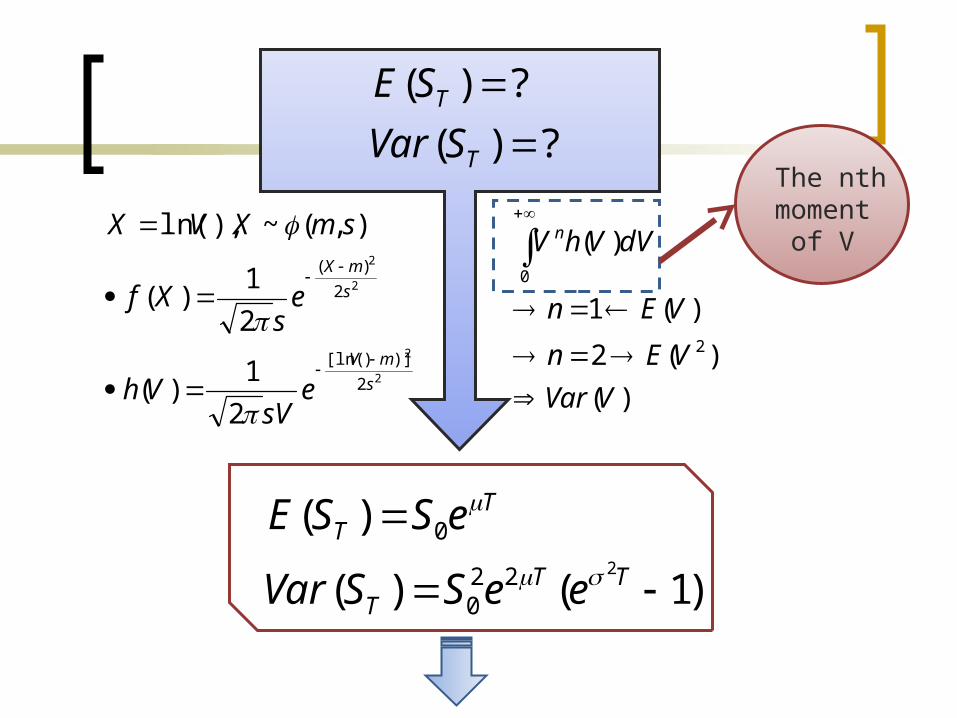
?)(
?)(
T
T
SVar
SE
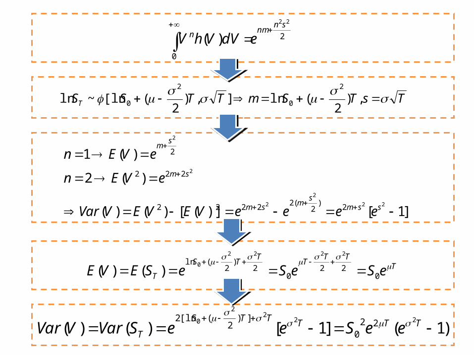
)1()(
)(222
0
0
TT
T
TT
eeSSVar
eSSE
2
2
2
2
2
)])[ln(
2
)(
2
1)(
2
1)(
),(~),ln(
s
mV
s
mX
esV
Vh
es
Xf
smXVX
)(
)(2
)(1
)(
2
0
VVar
VEn
VEn
dVVhV n
The nth moment of V

2
2
)(
2
2
2
2
)(
2
2][
2
][
0
2
][
22
2
2222
2
422
2
22
2
22
2
2
2
2
)(
2
1
2
1
2
1
2
2
snnmn
s
nsmxsnnm
s
snmns
s
nsmx
s
nxsmx
s
mxnx
xs
mx
x
nx
edVVhV
dxes
e
dxees
dxes
dxes
e
deese
e
2
2
2
2
2
)])[ln(
2
)(
2
1)(
2
1)(
),(~),ln(
s
mV
s
mX
esV
Vh
es
Xf
smXVX
xeV
xedee
xxx
ln1
0
42222222
22222
222)(
222)(
snmnsnxsmmxxnsmx
nxsmmxxnxsmx
2
0
22
)(sn
nmn edVVhV
TsTSmTTSST ,)2
(ln],)2
([ln~ln2
0
2
0
]1[)]([)()(
)(2
)(1
22
2
2
2
2
2)2
(22222
222
2
ssms
msm
sm
sm
eeeeVEVEVVar
eVEn
eVEn
TTT
TT
TS
T eSeSeSEVE
022
02
)2
(ln2222
0
)()(
)1(]1[)()(22
22
0 220
])2
([ln2
TTTTTS
T eeSeeSVarVVar

)1()(
)(222
0
0
TT
T
TT
eeSSVar
eSSE
Example 13.2A stock where the current price is $20An expected return of 20% per annumA volatility of 40% per annumAsk : the expected stock price, and the variance of the stock price, in 1year? 1
4.0
2.0
200
T
S
54.103)1(20)(
43.2420)(14.012.022
12.0
2
eeSVar
eSE
T
T

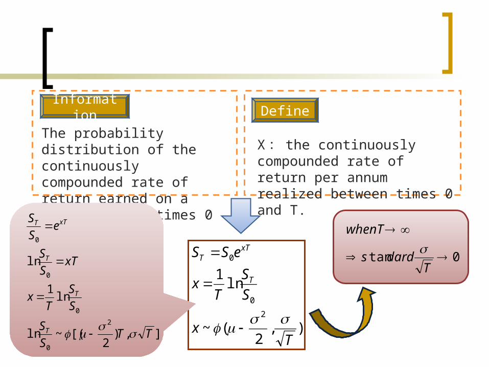
The distribution of the rate of return
Information Define
The probability distribution of the continuously compounded rate of return earned on a stock between times 0 and T.
X : the continuously compounded rate of return per annum realized between times 0 and T.
),2
(~
ln1
2
0
0
Tx
S
S
Tx
eSS
T
xTT
],)2
[(~ln
ln1
ln
2
0
0
0
0
TTS
S
S
S
Tx
xTS
S
eS
S
T
T
T
xTT
0tan
Tdards
whenT
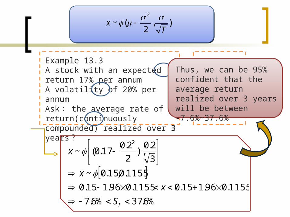
Example 13.3A stock with an expected return 17% per annumA volatility of 20% per annumAsk : the average rate of return(continuously compounded) realized over 3 years?
%6.37%6.7
1155.096.115.01155.096.115.0
1155.0,15.0~
3
2.0),
2
2.017.0(~
2
TS
x
x
x
05.0
3
2.0
17.0
T
Thus, we can be 95% confident that the average return realized over 3 years will be between-7.6%~37.6%
),2
(~2
Tx
The expected return

Expected return=E(R)= μ Expected return=E(x)=
ΔtμΔt,~S
ΔS ),2
(~2
Tx
2
2
TSSEeSSE TT
T 00 ln)](ln[)(
Assume In fact
)(
)][ln(
)ln()](ln[
)][ln()](ln[
0
0
RE
TS
SE
TSSE
SESE
T
T
TT
)2
)((
)(
)][ln(
)][ln()](ln[
2
0
xE
xE
TS
SE
SESE
T
TT
TSSEeSSE
TSSETS
S
TT
T
TT
00
2
0
2
0
ln)(ln)(
)2
(ln)][ln()2
()ln(
Arithmetic mean
Geometric mean

Example 13.4Initial investment of a mutual fund is $100The returns per annum report over the last five years:15%, 20%, 30%, -20%, 25%
Arithmetic mean>geometric meanArithmetic mean>geometric mean
%43.122
)1772.0(14.0)(
2)(
2
2
xE
xE
54.192)14.1(100 55 FV
Arithmetic mean
%145
%25%20%30%20%15
)(
RE
%4.12
1%)251%)(201(
%)301%)(201%)(151(
)(
5
xE
4.17925.18.0
3.12.115.11005
FV
Geometric mean

a. Estimating volatility from historical data
b. Trading days vs. calendar days
Volatility
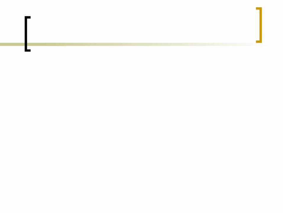
σ: a measure of our uncertainty about the returns provided by the stock
ΔtμΔt,~S
ΔS
),2
(~2
Tx
Between 15%~60%
The standard deviation of the return
The standard deviation of the percentage change in the stock price
With the square root of how far ahead we are looking
The standard deviation of the stock price in 4 weeks is approximately twice the standard deviation in 1 week.

Estimating volatility from historical data
Define
n+1 : number of observationsSi : stock price at end of ith interval, with i=0,1,2……,nτ: length of time interval in years
)ln(1
i
ii S
Su
2
11
2
1
2
)()1(
1
1
1
)(1
1
n
i i
n
i i
n
i i
unn
un
uun
s
s
s
),( iuVar
n2
Standard error( )
TT
S
ST ,2
~ln2
0
)(deviation standard iu

2
11
2
2
11
2
1
2
1
2
1
2
1 1 1
2112
1
22
1
2
)()1(
1
1
1
])(1
[1
1
])(1
)(2
[1
1
])()(2[1
1
)2(1
1
)(1
1
n
i i
n
i i
n
i i
n
i i
n
i
n
i i
n
i ii
n
i
n
i
n
i
n
i i
n
i iii
n
i ii
n
i i
unn
un
un
un
un
un
un
n
u
n
uuu
n
uuuun
uun
s
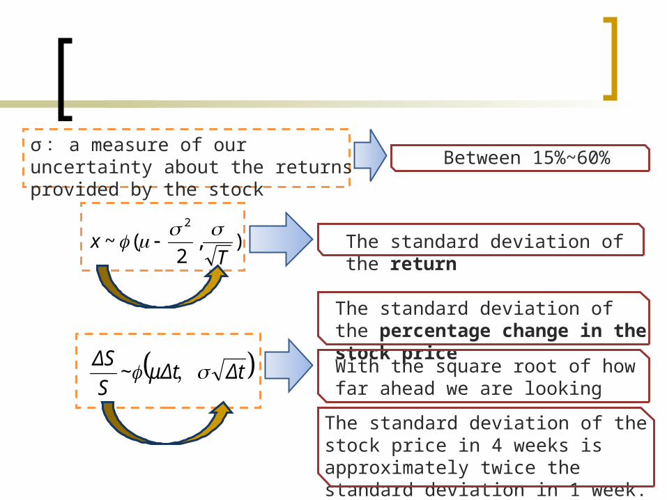
Trading days vs. calendar days
1. The variance of stock price returns between the close of trading on one day and the close of trading on the next day when there are no intervening nontrading days.
2. The variance of the stock price returns between the close of trading on Friday and close of trading on Monday.
Research
Reasonably expect
The first is a variance over a 1-day period. We might reasonably expect the second variance to be three times as great as the first variance.
The second variance to be, respectively, 22%, 19%, and 10.7% higher than the first variance.
In fact
‧ Volatility is much higher when the exchange is open for trading than when it is closed.‧Practitioners tend to ignore days when the exchange is closed.

annumper days
tradingofNumber
day trading
per Volatility
annumper
Volatility
252
matutityoption until days tradingofNumber T
The number of trading days in a years is usually assumed to be 252 for stocks.

00326.0
09531.0220
1
20
1
i i
i i
u
u
01216.0)120(20
09531.0
120
00326.0
)()1(
1
1
1
2
2
11
2
n
i i
n
i i unn
un
s
(year)193.0
2521
01216.0
s
031.0202
193.0
2
n
Standard error( )
00.20
10.20
90.20
75.20
90.20
90.20
00500.1ln
99282.0ln
00000.1ln

Concepts
derivationstock
A riskless portfolio
Return(portfolio)=risk-free interest rate(r)
No arbitrage opportunities
Example p.290△ c=0.4 S△→1. a long position in 0.4 shares 2. a short position in 1 call option
△ c=o.5△ S→1. an extra 0.1 share be purchased 2. for each call option sold
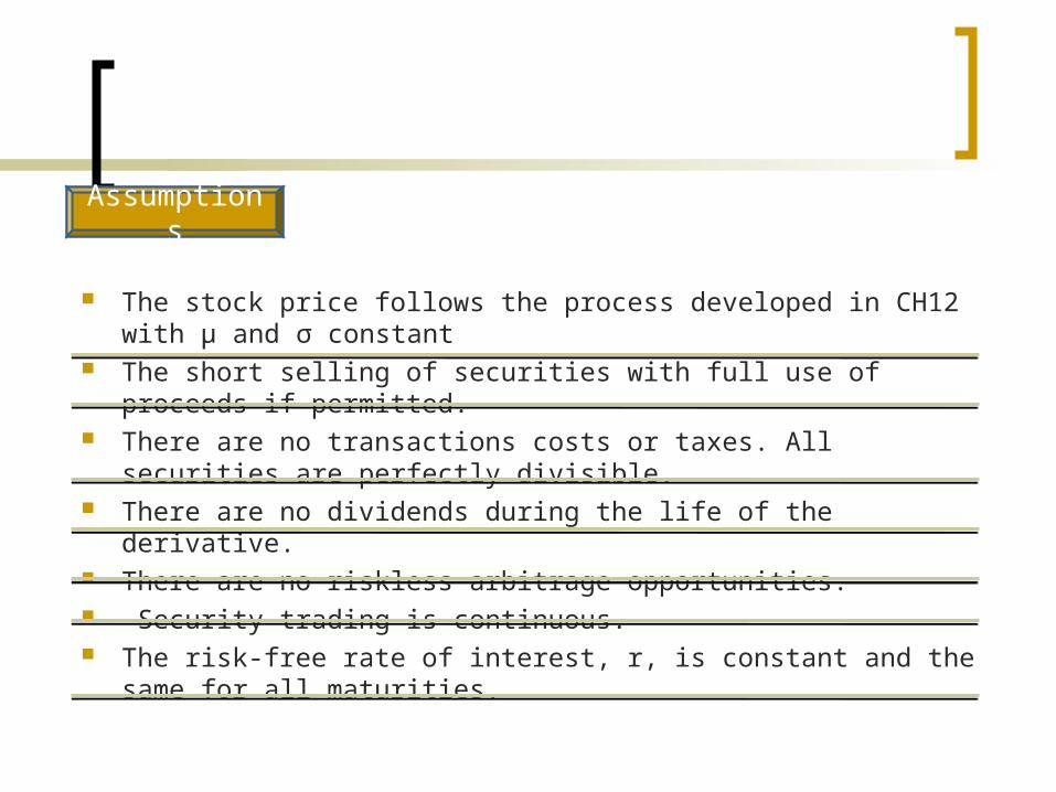
The stock price follows the process developed in CH12 with μ and σ constant
The short selling of securities with full use of proceeds if permitted. There are no transactions costs or taxes. All securities are perfectly
divisible. There are no dividends during the life of the derivative. There are no riskless arbitrage opportunities. Security trading is continuous. The risk-free rate of interest, r, is constant and the same for all
maturities.
Assumptions

Define
f : the price of the call option or other derivative contingent on S→f must be come function of S and t.π: the value of the portfolio
zStSS
zSS
ftS
S
f
t
fS
S
ff
222
2
2
1
equation
portfolio
S
f
-1 : derivative
: shares

process
tSS
f
t
f
zSS
ftS
S
fzS
S
ftS
S
ft
t
ftS
S
f
zStSS
fzS
S
ftS
S
f
t
fS
S
f
SS
ff
SS
ff
222
2
222
2
222
2
2
1
2
1
2
1
zStSS
zSS
ftS
S
f
t
fS
S
ff
222
2
2
1
This equation does not involve z△

222
2
222
2
222
2
2
1
2
1
2
1
SS
frS
S
f
t
frf
rSS
frfS
S
f
t
f
tSS
ffrtS
S
f
t
f
tr
△π=rπ t△The portfolio must instantaneously earn the same rate of return as other short-term risk-free securities.
tSS
f
t
f
22
2
2
2
1
SS
ff
(Black-Schiles-Merton differential equation)
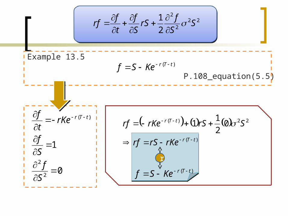
)( tTrKeSf
r
)( tTrKeSf Example 13.5
P.108_equation(5.5)
222
2
2
1S
S
frS
S
f
t
frf
0
1
2
2
)(
S
f
S
f
rKet
f tTr )(
22)( 02
11
tTr
tTr
rKerSrf
SrSrKerf
Application to Forward Contracts on a Stock
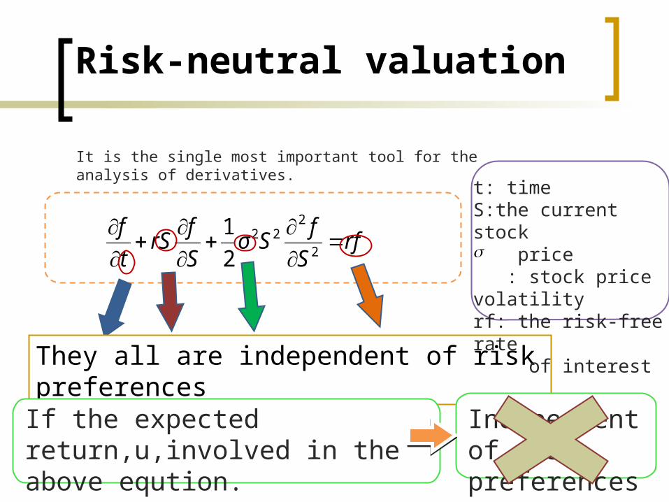
Risk-neutral valuation
rfS
fSσ
S
frS
t
f
2
222
2
1
It is the single most important tool for the analysis of derivatives.
Risk-neutral valuation
They all are independent of risk preferences
t: timeS:the current stock price : stock price volatilityrf: the risk-free rate of interest
If the expected return,u,involved in the above eqution.
Independent of risk preferences

Risk-neutral valuation
All investors are risk neutralAssumption:
The expected return of all investment asset is the risk-free rate of interest, r .
the expected return = rWhy
?Why
?

The risk-neutral investors do not require a premium to induce them to take risks.
1.
r=rf + s
Risk-neutral valuation
Reason:
present value expected value
Discount by r
2.
Any cash flow

How to use risk-neutral valuation
A derivative provides a payoff at one particular time.
step1
the expected return from the underlying asset is the risk-free interest rate, r.
Assume: Step2 Calculate the expected payoff from the derivative
Step3Discount the expected payoff at the risk-free interest rate.

Step3
Application to Forward Contracts on a Stock
Verify
Equation(5.5)
f = S 0 – Ke-rt A long forward contract
Maturity: time T Delivery price: K
A long forward contract
Maturity: time T Delivery price: K
step1Calculate:the value at maturity
ST - KST - K
ST : stock price at time T
Step2Calculate: the value at time 0
f = e-rT E(ST – K) = e-rTE(ST) –Ke-rT
(13.17)
Equation13.4
E(ST) = S0erT
E(ST) = S0erT
(13.18)
Substitute equation(13.18
) into (13.17)f = S0 – Ke-rt
step3
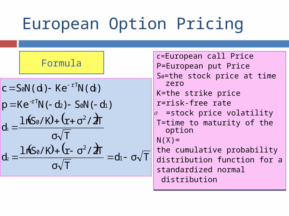
European Option Pricing
c=European call PriceP=European put PriceS0=the stock price at time zeroK=the strike pricer=risk-free rate =stock price volatilityT=time to maturity of the optionN(X)=the cumulative probability distribution function for a standardized normal distribution
c=European call PriceP=European put PriceS0=the stock price at time zeroK=the strike pricer=risk-free rate =stock price volatilityT=time to maturity of the optionN(X)=the cumulative probability distribution function for a standardized normal distribution
Tσd
Tσ
T/2σr/KSlnd
Tσ
T/2σr/KSlnd
)dN(S)dN(Kep
)N(dKe)N(dSc
1
20
20
102rT-
2rT
10
2
1
Formula
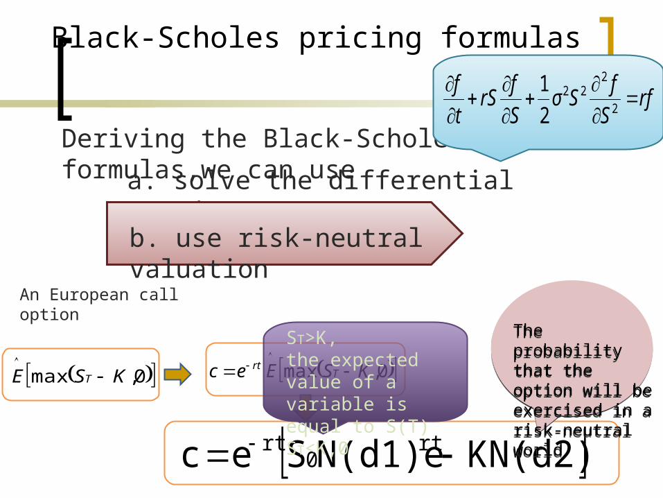
Black-Scholes pricing formulas
0,max KSE T 0,max KSEec T
rt
KN(d2)N(d1)eSec rt0
rt
ST>K,the expected value of a variable is equal to S(T)ST<K,0
The probability that the option will be exercised in a risk-neutral world
The probability that the option will be exercised in a risk-neutral world
a. solve the differential equation(13.16)
Deriving the Black-Scholes formulas,we can use
b. use risk-neutral valuation
rfS
fSσ
S
frS
t
f
2
222
2
1
An European call option

Derivation
If ln V~ N(m, w)E [max(V − K, 0)] = E(V )N(d1) − KN(d2)where
W
2/2W- ln[E(V)/K]d2
W
2/2Wln[E(V)/K]d1
E : expected value
Key result

Derivation
Define g(V) as the probability density function of V . It follows that
K
K)g(V)dV-(V K,0-VmaxE
• ln V ~ N(m, w) m=ln[E(V)] - w2/2 (13A.3)
Step1
(13A.2)
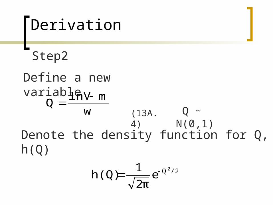
Derivation
Define a new variable
(13A.4) Q ~ N(0,1)
Denote the density function for Q, h(Q)
/2Q2
e2π
1h(Q)
w
mlnVQ
Step2

Derivation
Step3Using equation(13A.4) to convert the expression on the right-hand side of equation(13A.2)from an integral over V to an integral over Q
QdQhK)(eK,0VmaxEm)/w(lnK
mQw
m)/w(lnKm)/w(lnK
mQw QdQhKQdQheK,0VmaxE
(13A.5)

Derivation
/22m2QwQmQw 2
e2π
1Qhe
/2w2mwQ 22
e2π
1
/2wQ/2wm
2
2
e2π
e
w)h(Qe /2wm 2
QdQhKe wm
m)/w(lnKm)/w(lnK
2/ w)dQ-h(QK,0 - VmaxE2
step4
(13A.6)
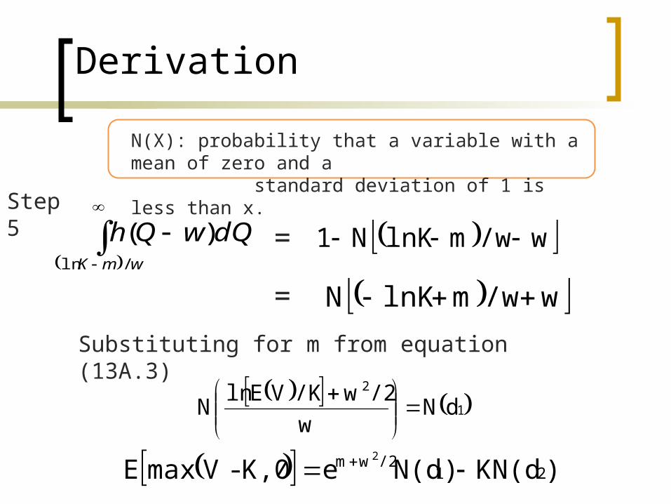
Derivation
w/wmlnKN1
w/wmlnKN
12
dNw
/2w/KVElnN
)KN(d)N(deK,0 - VmaxE 21/2wm 2
N(X): probability that a variable with a mean of zero and a standard deviation of 1 is less than x.
wmK
dQwQh/ln
)( =
=
Substituting for m from equation (13A.3)
Step5

T
2//KSln2
T
2//KSln1
2O
2O
d
d
Tr
Tr
Properties of the Black-Scholes Formulas
When stock price becomes very large
N(d1)1N(d2)1
N(-d1)0N(-d2)0
d1.d2 become very largeN(-d1)=1-N(d1)N(-d2)=1-N(d2)

)N(dKe)N(dSc 2rT
10 d1)N(Sd2)N(Kep 0
rT
price p approaches zero
So- Ke-rt
very similar to a forward contract with delivery price K.
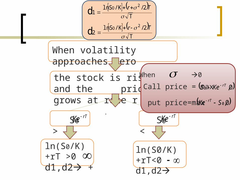
When volatility approaches zero
rTeS 0
the stock is riskless and the price grows at rate r to .
S0 > rTKe S0 < rTKe
ln(S0/K)+rT >0d1,d2 + ln(S0/K)+rT<0
d1,d2
T
2//KSln2
T
2//KSln1
2O
2O
d
d
Tr
Tr
Call price = max put price=max
When 0 0,rTO KeS
0,0SKe rT

Cumulative normal distribution function
2 3 4 51 2 3 4 51 ( )( ) 0
( )1 ( ) 0
N x a k a k a k a k a k if xN x
N x if x
1
, 0.23164191
kx
1 0.319381530a 2 0.356563782a 3 1.781477937a
4 1.821255978a 5 1.330274429a
2 21( )
2xN x e

Example
Example 13.6The stock price 6months from the expiration of an option is $ 42The exercise price of the option is $40The risk-free interest rate is 10%The volatility of 20% per annum
5.0
2.0
1.0
40
420
T
r
K
S
6278.0
0.50.2
5.02/2.00.142/40ln2
2
d
Ke-rt =40e-0.1*0.5 = 38.049
7693.0
0.50.2
5.02/2.00.142/40ln1
2
d
c=42N(0.7693)-38.049N(0.6278) p= 38.049 N(-0.6278)-38.049N(-0.7693)
N(0.7693)=0.7791 N(-0.7693)=0.2209N(0.6278)=0.7349N(0.-6278)=0.2651

Implied volatilities
In the Black-Scholes pricing formulas
the volatility of the stock price.
Functions:a.Monitor the market’s opinion about the volatility of particular stock.b. From actively traded option on a certain asset,Traders use to calculate the appropriate volatility for pricing a less actively traded option on the same stock.
calculated by option price observed in the market.
We can’t find
We can’t find

σ=0.2 c=1.76 too low
σ=0.3 c=2.1 too high
σ=0.25 too high
European call option (No dividend)C=1.875So= 21K= 20r=10% (per annum)T=0.25Ask: σ =??Implied volatility
)N(dKe)N(dSc 2rT
10
How to do?? Iterative search
C is an increasing function of σ
σ lies between 0.2 and 0.25.In this example, the implied volatilities is 0.235

Dividends
Assumption:
a.The amount and timing of the dividends during the life of an option can be predicted with certainty.
b.The date on which the dividend is paid should be assumed to be the ex-dividend date.
c.On this date the stock price declines by the amount of the dividend.
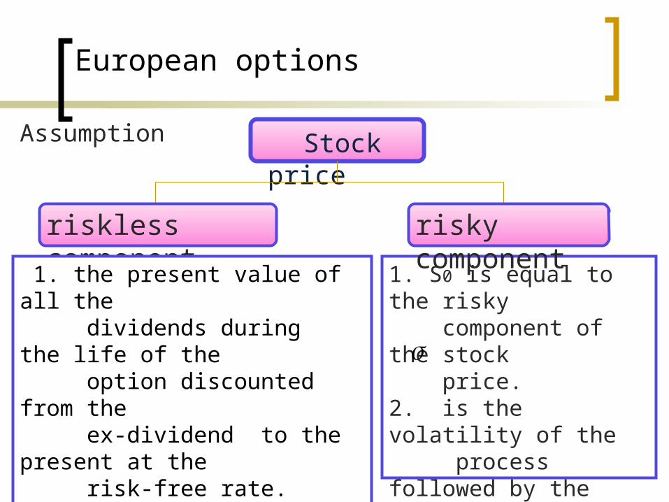
European options
Assumption Stock price
riskless component risky component
1. the present value of all the dividends during the life of the option discounted from the ex-dividend to the present at the risk-free rate. 2.By the time the option matures, the dividends will have been paid and the this part will no longer exist.
1. S0 is equal to the risky component of the stock price.2. is the volatility of the process followed by the risky component

Example 13.8European call option on a stockEx-dividend dates in two months and five monthsThe dividend is expected to be $0.5The current share price is$40The exercise price is $40The risk-free interest rate is 9%The volatility of 30% per annumTime maturity is six monthsASK:European call option price??
9.0
5.0
3.0
40
5.0
400
r
T
K
D
S

Calculate the present value of the dividends 0.5e-0.1667*0.09 + 0.5e-0.4167*0.09 = 0.9741
2/122/12 5/12
5/12
So minus the present value of the dividends 40 - 0.9741=39.0259
Use Black-Scholes pricing formulas d1=0.2017 N(d1)=0.58 d2=-0.0104 N(d2)=0.4959
Call price: 39.0259 × 0.58 - 40e-0.5*0.09 ×0.4959 =3.67
T
2//KSln2
T
2//KSln1
2O
2O
d
d
Tr
Tr
)N(dKe)N(dSC 21rT
0

American Option
The dividends corresponding to these times will be denoted by D1,D2 …,Dn,respectively.
Assumption
When there are dividends, it is optimal to exercise only at a time immediately before the stock goes ex-dividend.
n ex-dividend dates are anticipated and they are at times t1,t2 …tn, with(t1<t2< …<tn)
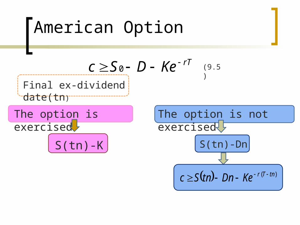
American Option
rTKeDSc 0 (9.5)
Final ex-dividend date(tn)
The option is exercised
S(tn)-K
The option is not exercised
S(tn)-Dn
)( tnTrKeDntnSc

American Option
If )()( KtnSKeDntnS tnTr
)1( )( tnTreKDn then
It cannot be optimal to exercise at time tn
)( 11 titr ieKDi
It is not optimal to exercise immediately prior to time ti
It can be optimal to exercise at time tn)1( )( tnTreKDn
If
Very large
T-tn is small