![Synthesis and Characterization of [n]Cumulenes ...](https://static.fdocument.pub/doc/165x107/58a181de1a28abb24d8c126c/synthesis-and-characterization-of-ncumulenes-.jpg)
SYNTHESIS, CHARACTERIZATION, AND THERMOPHYSICAL PROPERTIES...
187
SYNTHESIS, CHARACTERIZATION, AND THERMOPHYSICAL PROPERTIES OF MAGHEMITE (γ-Fe 2 O 3 ) NANOFLUIDS WITH AND WITHOUT MAGNETIC FIELDS EFFECT IRWAN NURDIN FACULTY OF ENGINEERING UNIVERSITY OF MALAYA KUALA LUMPUR 2016
Transcript of SYNTHESIS, CHARACTERIZATION, AND THERMOPHYSICAL PROPERTIES...

SYNTHESIS, CHARACTERIZATION, AND
THERMOPHYSICAL PROPERTIES OF MAGHEMITE
(γ-Fe2O3) NANOFLUIDS WITH AND WITHOUT
MAGNETIC FIELDS EFFECT
IRWAN NURDIN
FACULTY OF ENGINEERING
UNIVERSITY OF MALAYA
KUALA LUMPUR
2016

SYNTHESIS, CHARACTERIZATION, AND
THERMOPHYSICAL PROPERTIES OF MAGHEMITE
(γ-Fe2O3) NANOFLUIDS WITH AND WITHOUT
MAGNETIC FIELDS EFFECT
IRWAN NURDIN
THESIS SUBMITTED IN FULFILMENT OF THE
REQUIREMENTS FOR THE DEGREE OF DOCTOR OF
PHILOSOPHY
FACULTY OF ENGINEERING
UNIVERSITY OF MALAYA
KUALA LUMPUR
2016
ii
UNIVERSITY OF MALAYA
ORIGINAL LITERARY WORK DECLARATION
Name of Candidate: Irwan Nurdin (I.C/Passport No: A5747183)
Registration/Matric No: KHA 090058
Name of Degree: Doctor of Philosophy
Title of Project Paper/Research Report/Dissertation/Thesis (“this Work”):
Synthesis, Characterization, And Thermophysical Properties of Maghemite
(γ-Fe2O3) Nanofluids With And Without Magnetic Fields Effect
Field of Study: Nanomaterials
I do solemnly and sincerely declare that:
(1) I am the sole author/writer of this Work;
(2) This Work is original;
(3) Any use of any work in which copyright exists was done by way of fair dealing
and for permitted purposes and any excerpt or extract from, or reference to or
reproduction of any copyright work has been disclosed expressly and
sufficiently and the title of the Work and its authorship have been
acknowledged in this Work;
(4) I do not have any actual knowledge nor do I ought reasonably to know that the
making of this work constitutes an infringement of any copyright work;
(5) I hereby assign all and every rights in the copyright to this Work to the
University of Malaya (“UM”), who henceforth shall be owner of the copyright
in this Work and that any reproduction or use in any form or by any means
whatsoever is prohibited without the written consent of UM having been first
had and obtained;
(6) I am fully aware that if in the course of making this Work I have infringed any
copyright whether intentionally or otherwise, I may be subject to legal action
or any other action as may be determined by UM.
Candidate’s Signature Date:
Subscribed and solemnly declared before,
Witness’s Signature Date:
Name:
Designation:

iii
ABSTRACT
Synthesis, characterization, and thermophysical properties of maghemite nanofluids
have been studied with and without magnetic fields effect. The objectives of study are to
synthesize maghemite nanoparticles and their characterization using various methods, to
prepare stable maghemite nanofluids, and measurement of thermophysical properties of
maghemite nanofluids with and without external magnetic fields effect. Maghemite
nanoparticles were synthesized by chemical co-precipitation method with different
concentrations of nitric acid. Maghemite nanofluids were then prepared and the stability
of the nanofluids were characterized by zeta potential and dynamic light scattering at
different pH and time of storage. Lastly, measurements of thermal conductivity, viscosity,
and electrical conductivity of maghemite nanofluids were taken at various particle
volume fraction, temperatures, with and without strengths of magnetic fields. Results
show that spherical shape of superparamagnetic maghemite nanoparticles with good
thermal and suspensions stability was successfully synthesized within the size range of
9.3 to 14.7 nm. The stability of maghemite nanofluids show that the suspensions remain
stable at acidic condition with zeta potential value of 44.6 mV at pH 3.6 and at basic
condition with zeta potential -46.2 mV at pH 10.5. The isoelectric point of the maghemite
nanoparticles suspensions is obtained at pH 6.7. The maghemite nanofluids remains
stable after eight months of storage. The thermal conductivity of maghemite nanofluids
linearly increases with increasing of particle volume fraction, temperature, and magnetic
fields strengths. The kinematic viscosity of maghemite nanofluids increases with
increasing of particle volume fraction and magnetic fields and decrease with increasing
of temperature. Electrical conductivity of maghemite nanofluids increases with increasing
of particle volume fraction and temperature and no effect with magnetic fields.

iv
ABSTRAK
Sintesis, pencirian, dan sifat termofizikal bendalir maghemite nano telah dikaji dengan
dan tanpa kesan medan magnet. Objektif kajian ini adalah untuk mensintesis zarah
maghemite nano dan menjalankan pencirian dengan menggunakan pelbagai kaedah,
menyediakan bendalir maghemite nano yang stabil, dan pengukuran ciri-ciri termofizikal
bendalir maghemite nano dengan dan tanpa pengaruh medan magnetik luaran. Sintesis
zarah maghemite nano dengan menggunakan kaedah co-pemendakan kimia. Kepekatan
asid nitrik yang berbeza digunakan sebagai pembolehubah, kemudian penyediaan
bendalir maghemite nano yang stabil yang dicirikan dengan mengukur keupayaan zeta
dan “dynamic light scattering” pada pH dan masa simpanan yang berbeza. Akhirnya,
pengukuran kekonduksian terma, kelikatan, dan kekonduksian elektrik bendalir
maghemite nano pada pelbagai suhu, kepekatan zarah maghemite nano, dengan dan tanpa
kekuatan medan magnetik luar. Hasil uji kaji menunjukkan superparamagnetik zarah
maghemite dengan bentuk sfera dan kestabilan haba dan suspensi yang baik dan saiz
dalam julat 9.3 – 14.7 nm telah berjaya dihasilkan. Bendalir maghemite nano yang stabil
menunjukkan ia berada di keadaan asid dengan nilai keupayaan zeta 44.6 mV pada pH
3.6 dan pada keadaan bes dengan nilai keupayaan zeta -46.2 mV pada pH 10.5. Takat
isoletrik pula di perolehi pada pH 6.7. Bendalir maghemite nano masih berada dalam
keadaan stabil selepas lapan bulan. Kekonduksian terma bendalir maghemite nano adalah
linear meningkat dengan peningkatan kepekatan zarah, suhu dan medan magnet.
Kelikatan kinematik bendalir maghemite nano adalah meningkat dengan peningkatan
kepekatan jumlah zarah dan medan magnet dan menurun dengan peningkatan suhu.
Manakala, kekonduksian elektrik adalah meningkat dengan peningkatan kepekatan zarah,
dan suhu dan tidak berkesan dengan medan magnet.

v
ACKNOWLEDGEMENTS
With deep regards and profound respect, I would like to express my sincere thanks and
gratitude toward Prof. Dr. Mohd Rafie Johan and Prof. Dr. Iskandar Idris Yaacob for
introducing the present research topic and for their inspiring guidance, constructive
criticism, and valuable suggestion throughout this research work. It would have not been
possible for me to bring out this thesis without their help and constant encouragement.
Special thanks to my colleague, Ms. Yusrini Marita, Mrs. Ang Bee Chin, Ms. Siti
Hajar, Mrs. Fatihah, Mr. Shahadan Mohd Suan, Mrs. Aliya, Mrs. Yusliza, Ms. Syima
Razali, Mrs. Asmalina, Mrs. Mariah and Ms. Nadia in sharing their knowledge and ideas
with me. Besides that, sincerest appreciation goes to Faculty of Engineering, University
of Malaya for providing all the facilities in the Mechanical Department and laboratories.
Not forgetting also, the dedicated laboratory assistant Mr. Mohd Said Sakat, Mr. K.
Kandasamy and Mr. Suhaimi, Mrs. Norzirah, and Ms. Aida Nur Izzaty for giving their
full co-operation while using the equipments.
Last but not least, awards of thanks to my father Nurdin Abidin (alm), my mother,
Nuriah Husin and lovely family members and my wife Mrs Nurliza Idris and my children
Thariq Irza and Tsaqif Aufa Irza who give me full support in making this research work
a success. Thanks for sharing my hard time.
Appreciate the efforts and contributions shared by individuals whose names are not
mentioned above.
Thank you so much.

vi
TABLE OF CONTENTS
Abstract………………………………………………………………………………… iii
Abstrak………………………………………………………………………………… iv
Acknowledgements…………………………………………………………………….. v
Table of Contents………………………………………………………………….........vi
List of Figures …………………………………………………………………………..ix
List of Tables…………………………………………………………………………..xiii
List of Symbols and Abbreviations……………………………………………………..xv
List of Appendices………………………………………………….…………..……..xvii
CHAPTER I: INTRODUCTION...................................................................................1
1.1 Background………………………………………………………………………..1
1.2 Problem Statement………………………………………………………………...3
1.3 Objectives………………………………………………………………………….4
1.4 Research Scope and Limitation …………………………………………………...4
1.5 Significant of Research……………………………………………………………5
1.6 Thesis Organization……………………………………………………………….5
CHAPTER II: LITERATURE REVIEWS…………………………………………...7
2.1 Nanofluids…………………………………………………………………………7
2.1.1 Fundamental of nanofluids………………………………………………...7
2.1.2 Impact and potential benefit of nanofluids…………………………………9
2.1.3 Potential application of nanofluids………………………………………..10
2.2 Synthesis of Maghemite Nanoparticles ………………………………………….14
2.3 Application of Maghemite Nanofluids…………………………………………..17
2.3.1 Magnetic resonance imaging……………………………………………..17
2.3.2 Magnetic separation………………………………………………………18
2.3.3 Nanocatalysis……………………………………………………………..19

vii
2.3.4 Thermal engineering……………………………………………………...19
2.3.5 Environmental ...………………………………………...……………….21
2.4 Magnetism and Magnetic Properties of Nanoparticles…………………………..22
2.5 Stability of Maghemite Nanofluids……………………………………………….29
2.6 Thermophysical Properties……………………………………………………….32
2.6.1 Thermal conductivity……………………………………………………..32
2.6.2 Viscosity………………………………………………………………….43
2.6.3 Electrical Conductivity…………………………………………………...47
CHAPTER III: METHODOLOGY……………………………………….................54
3.1 Materials………………………………………………………………………….54
3.2 Synthesis of Maghemite Nanoparticles ………………………………………….55
3.3 Preparation of Maghemite Nanofluids……………………………………………56
3.4 Thermophysical Properties Measurement………………………………………..57
3.4.1 Preparation of Maghemite Nanofluids……………………………………57
3.4.2 Procedure…………………………………………………………………57
3.4.3 Measurement……………………………………………………………..59
3.5 Characterization Technique ……………………………………………………...61
3.5.1 X-Ray Diffractometer (XRD)…………………………………………….61
3.5.2 Transmission Electron Microscopy (TEM)………………………………63
3.5.3 Alternating Gradient Magnetometer (AGM)……………………………..66
3.5.4 Thermogravimetry Analysis (TGA)……………………………………...67
3.5.5 Dynamic Light Scattering (DLS)…………………………………………68
3.5.6 Zeta Potential Analysis ………………………………………………….71
CHAPTER IV: RESULTS AND DISCUSSIONS ………………………………….76
4.1 Synthesis of Maghemite Nanoparticle……………………………………………76
4.2 Stability Monitoring of Maghemite Nanofluids………………………………….88
viii
4.2.1 Effect of pH……………………………………………………………....88
4.2.2 Effect of time……………………………………………………………..90
4.3 Thermophysical Properties of Maghemite Nanofluids…………………………..93
4.3.1 Effect of particle volume fraction………………………………………..93
4.3.2 Effect of temperature…………………………………………………....103
4.3.3 Effect of magnetic fields …………………………………………….…112
CHAPTER V: CONCLUSIONS AND RECOMMENDATIONS………………..131
5.1 Conclusions……………………………………………………………………..131
5.2 Recommendations………………………………………………………………133
References……………………………...………………………………………...…...135
List of Publication and Papers Presented………………………………………………148
Appendices ……………………………………………………………………………149

ix
LIST OF FIGURES
Figure 2.1: Magnetic field lines in a magnet bar……………………………………….22
Figure 2.2: Behavior of superparamagnetic particles with and without
the presence of an applied external magnetic field………………………...25
Figure 2.3: Magnetization Curve……………………………………………………….25
Figure 2.4: Initial Permeability of Magnetization Curve……………………………….27
Figure 3.1: Flowchart of research methodology………………………………………..55
Figure 3.2: Flowchart of synthesis of maghemite nanoparticle…………………………56
Figure 3.3: Schematic of experimental set up for thermal conductivity…………………58
Figure 3.4: Schematic of experimental set up for viscosity measurement………………58
Figure 3.5: Schematic of experimental set up for electrical conductivity……………….59
Figure 3.6: Schematic of calibrated glass capillary viscometer…………………………61
Figure 3.7: Diffraction of x-rays by atoms from two parallel planes……………………62
Figure 3.8: Schematic Diagram of TEM………………………………………………...65
Figure 3.9: Schematic of sample in AGM analysis ………………………………….67
Figure 3.10 : Schematic representation of zeta potential……………………………….72
Figure 3.11: Stern model of zeta potential theory………………………………………74
Figure 4.1: XRD pattern of maghemite nanoparticle ………………………………….77
Figure 4.2: Particle size and lattice parameters from XRD calculations……………….79
Figure 4.3: TEM images of maghemite nanoparticles for samples MNA2…………….80
Figure 4.4: Particle distribution for maghemite nanoparticles for samples MNA2……...80
Figure 4.5: TEM images of maghemite nanoparticles for samples MNA4……………...81
Figure 4.6: Particle distribution for maghemite nanoparticles for samples MNA4……...81
Figure 4.7: TEM images of maghemite nanoparticles for samples MNA6……………...82
Figure 4.8: Particle distribution for maghemite nanoparticles for samples MNA6……...82
Figure 4.9: TEM images of maghemite nanoparticles for samples MNA8……………...83

x
Figure 4.10: Particle distribution for maghemite nanoparticles for samples MNA8…….83
Figure 4.11: TEM images of maghemite nanoparticles for samples MNA10…………...84
Figure 4.12: Particle distribution for maghemite nanoparticles for samples MNA10…...84
Figure 4.13: Magnetization curve of maghemite nanoparticles for all samples…………85
Figure 4.14: TGA thermogram of maghemite nanoparticles for all samples……………86
Figure 4.15: LS measurement of maghemite nanoparticle for all samples………………87
Figure 4.16: Zeta potential measurement of maghemite nanoparticles for all samples….88
Figure 4.17: Particle size and zeta potential measurement of maghemite
nanofluids at different pH………………………………………………...90
Figure 4.18: Particle size distribution of maghemite nanoparticle from
DLS measurement…………………….………………………………….91
Figure 4.19 : Zeta potential curves of maghemite nanofluids…………………………...92
Figure 4.20: Thermal conductivity of maghemite nanofluids as a function
of particle volume fraction at different temperature……………………...94
Figure 4.21: Thermal conductivity ratio of maghemite nanofluids as a function
of particle volume fraction at different temperature………………………95
Figure 4.22: Enhancement of thermal conductivity of maghemite nanofluids
as a function of particle volume fraction at different temperature………...96
Figure 4.23: Viscosity of maghemite nanofluids as a function of particle
volume fraction at different temperature………………………………...98
Figure 4.24: Kinematic viscosity ratio of maghemite nanofluids as a
function particle volume fraction at different temperature………………99
Figure 4.25: Enhancement of kinematic viscosity of maghemite nanofluids
as a function of particle volume fraction at different temperature………99
Figure 4.26: Electrical conductivity of maghemite nanofluids as a function
of particle volume fraction at different temperature……………………..102
Figure 4.27: Enhancement of electrical conductivity of maghemite nanofluids
as a function of particle volume fraction at different temperature……….103
Figure 4.28: Thermal conductivity of maghemite nanofluids as a function of
temperature at different particle volume fraction………………………..104
Figure 4.29: Thermal conductivity ratio of maghemite nanofluids as a
function of temperature at different particle volume fraction……………105
xi
Figure 4.30: Enhancement of thermal conductivity of maghemite as a
function of temperature at different particle volume fraction……………106
Figure 4.31: Kinematic viscosity of maghemite nanofluids as a function
of temperature at different particle volume fraction……………………..107
Figure 4.32: Kinematic viscosity ratio of maghemite nanofluids as
a function of temperature at different particle volume fraction…………109
Figure 4.33: Decreasing of kinematic viscosity of maghemite nanofluids as a
function of temperature at different particle volume fraction……………109
Figure 4.34: Electrical conductivity of maghemite nanofluids as a
function of temperature at different particle volume fraction……………110
Figure 4.35: Enhancement of electrical conductivity of maghemite nanofluids
as a function of temperature at different particle volume fraction………111
Figure 4.36: Thermal conductivity of maghemite nanofluids at different parallel
magnetic fields strength ………………………………………………...114
Figure 4.37: Thermal conductivity ratio of maghemite nanofluids as a function
of magnetic field parallel to the temperature gradient at different
volume fraction………………………………………………………….115
Figure 4.38: Thermal conductivity enhancement of maghemite nanofluids
as a function of magnetic field parallel to the temperature
gradient at different volume fraction…………………………………….116
Figure 4.39: Thermal conductivity of maghemite nanofluids at different
perpendicular magnetic fields strength………………………………….117
Figure 4.40: Thermal conductivity of maghemite nanofluids as a function
of magnetic field perpendicular to the temperature gradient
at different volume fraction……………………………………………...119
Figure 4.41: Thermal conductivity enhancement of maghemite nanofluids a as
a function of magnetic field perpendicular to the temperature
gradient at different volume fraction…………………………………….119
Figure 4.42: Kinematic viscosity of maghemite nanofluids as a function of
different parallel magnetic fields strength at 25 oC for
different particle volume fraction………………………………………..120
Figure 4.43: Kinematic viscosity ratio of maghemite nanofluids as a function
of different parallel magnetic fields strength at 25 oC for
different particle volume fraction…………………………………….....121
Figure 4.44: Kinematic viscosity enhancement of maghemite nanofluids as a
function of different parallel magnetic fields strength at 25 oC
for different particle volume fraction……………………………………122

xii
Figure 4.45: Kinematic viscosity of maghemite nanofluids at different
perpendicular magnetic fields strength at 25 oC…………………………124
Figure 4.46: Kinematic viscosity ratio of maghemite nanofluids as a function
of magnetic field perpendicular to the temperature
gradient at different volume fraction…………………………………….125
Figure 4.47: Kinematic viscosity enhancement of maghemite nanofluids
as a function of magnetic field perpendicular to the temperature
gradient at different volume fraction…………………………………….126
Figure 4.48: Electrical conductivity of maghemite nanofluids
as a function of magnetic field parallel to the temperature
gradient at different volume fraction…………………………………….127
Figure 4.49: Electrical conductivity enhancement of maghemite nanofluids
as a function of magnetic field perpendicular to the temperature
gradient at different volume fraction…………………………………….130

xiii
LIST OF TABLES
Table 2.1: Thermal conductivity of various materials at 300 K………………………..8
Table 2.2: Summary of models developed for thermal conductivity of nanofluids…...37
Table 4.1: Particles size, magnetic property, zeta potential and temperature
stability of maghemite nanoparticles…………………………………..…..76
Table 4.2: Comparison between XRD characteristic peaks of
the sample and standard ………………………………………………….77
Table 4.3: Indexing of the Miller indices of maghemite sample..……………………...78
Table 4.4: Lattice parameter calculation…………….…………………………….…..78
Table 4.5: Particle size and zeta potential measurement at various
time of storage………………………………………………………..……92
Table 4.6: Thermal conductivity of maghemite nanofluids at different
particle volume fraction ………………………………………………….94
Table 4.7: Regression line equation of thermal conductivity of maghemite
nanofluids as a function of particle volume fraction………………………95
Table 4.8: Kinematic viscosity of maghemite nanofluids at
different particle concentration ………………………………..………...97
Table 4.9: Regression line equation of kinematic viscosity of maghemite
nanofluids as a function of particle concentration ………………... 98
Table 4.10: Electrical conductivity of maghemite nanofluids as a function
of particle volume fraction at different temperature………………………101
Table 4.11: Regression line equation of electrical conductivity of maghemite
nanofluids at various particle volume fraction………………………….. 102
Table 4.12: Thermal conductivity of maghemite nanofluids at different temperature…104
Table 4.13: Regression line equation of thermal conductivity of
maghemite nanofluids as a function of temperature……………………..105
Table 4.14: Kinematic viscosity of maghemite nanofluids as a function of
temperature at different particle volume fraction………………………....107
Table 4.15: Regression line equation of kinematic viscosity of maghemite
nanofluids as a function of temperature at different
particle volume fraction…………………………………………………..108
Table 4.16: Electrical conductivity of maghemite nanofluids as a
function of temperature at different particle volume fraction……………110

xiv
Table 4.17: Regression line equation of electrical conductivity of
maghemite nanofluids as a function of temperature……………………...111
Table 4.18: Thermal conductivity of maghemite nanofluids at
different parallel magnetic fields strength……………………………….113
Table 4.19: Regression line equation of thermal conductivity of maghemite
nanofluids at different parallel magnetic fields strength…………………114
Table 4.20: Thermal conductivity of maghemite nanofluids at
different perpendicular magnetic fields strength…………………………117
Table 4.21: Regression line equation of thermal conductivity of maghemite
nanofluids at different perpendicular magnetic fields strength…………...118
Table 4.22: Kinematic viscosity of maghemite nanofluids as a function of
different parallel magnetic fields strength at 25 oC for
different particle volume fraction…………………………………………119
Table 4.23: Regression line equation of kinematic viscosity of maghemite
nanofluids at different parallel magnetic fields strength…………………..121
Table 4.24: Kinematic viscosity of maghemite nanofluids at
different perpendicular magnetic fields strength………………………….123
Table 4.25: Regression line equation of kinematic viscosity of maghemite
nanofluids at different perpendicular magnetic fields strength………..….124
Table 4.26: Electrical conductivity of maghemite nanofluids at
different parallel magnetic fields strength………………………………...127
Table 4.27: Regression line equation of electrical conductivity of maghemite
nanofluids at different parallel magnetic fields strength…………………..128
Table 4.28: Electrical conductivity of maghemite nanofluids at different
perpendicular magnetic fields strength……………………………………129
Table 4.29: Regression line equation of electrical conductivity of maghemite
nanofluids at different parallel magnetic fields strength…………………..130

xv
LIST OF SYMBOLS AND ABBREVIATIONS
Symbol or
Abbreviations
Meaning Unit (SI)
H
B
µo
µ
µr
M
Ms
knf
kbf
kp
ϕ
ψ
µ
µbf
µnf
EDL
σm
σo
α
XRD
TEM
AGM
TGA
Magnetic fields strength
Magnetic induction
Permeability of free space
Permeability of materials
Relative permeability
Magnetization
Saturation magnetization
Thermal conductivity of nanofluids
Thermal conductivity of base fluids
Thermal conductivity of particle
Particle volume fraction
Particle sphericity
Viscosity of suspensions
Viscosity of base fluids
Viscosity of nanofluids
Electrical double layer
Electrical conductivity
Electrical conductivity of base fluids
Electrical conductivity ratio
X-Ray diffraction
Transmission electron spectroscopy
Alternating gradient magnetometer
Thermogravimetry analysis
Tesla (T)
A/m
4p x 10-7
-
-
Weber (Wb)
emu/g
W/mK
W/mK
W/mK
%
-
cst
cst
cst
-
S/m
S/m
-
-
-
-
-

xvi
DLS
mp
mf
ρl
ρp
T
ξ
d
D
Dynamic light scattering
Mass of particle
Mass of fluids
Density of fluids
Density of particle
Temperature
Zeta potential
Diameter of particle
Translational diffusion coefficient
-
g
g
g/mL
g/mL
K
mV
cm

xvii
LIST OF APPENDICES
Appendix A: Profile fit for XRD analysis……………..…...…..................................149
Appendix B: TEM image of maghemite nanoparticle…………..…………………..155
Appendix C: TGA thermogram of maghemite nanoparticle……..………………….157
Appendix D: DLS measurement of maghemite nanoparticle…..................................158
Appendix E: Zeta Potential measurement of maghemite nanoparticle……………...158
Appendix F: Thermal conductivity measurements at various particle
volume fraction…………………………………………………….…159
Appendix G: Thermal conductivity measurements at various temperature…….…...159
Appendix H: Thermal conductivity measurements at various parallel
magnetic fields………………………………………..………………160
Appendix I: Thermal conductivity measurements at various perpendicular
magnetic fields…………..…………………………………………….161
Appendix J: Kinematic viscosity measurements at various particle
volume fraction…………………….………………………………….162
Appendix K: Kinematic viscosity measurements at various temperature…..……….163
Appendix L: Kinematic viscosity measurements at various parallel
magnetic fields………………………………………………………...164
Appendix M: Kinematic viscosity measurements at various perpendicular
magnetic fields………………………………………………………...165
Appendix N: Electrical conductivity measurements at various particle
volume fraction……………………….……………………………….166
Appendix O: Electrical conductivity measurements at various temperature………...167
Appendix P: Electrical conductivity measurements at various parallel
magnetic fields…………………...…………………………………....168
Appendix Q: Electrical conductivity measurements at various perpendicular
magnetic fields………………………………………………………...169
1
INTRODUCTION
This chapter describes the background, objectives, scope and limitation and the
significant research of study on synthesis, characterization, and thermophysical properties
of maghemite nanofluids with and without magnetic field effects.
1.1 Background
Understanding and control of the synthesis and properties of engineered materials at
scales similar to those of atoms and molecules is of utmost importance as this field of
nanotechnology makes its progress in today’s science. The uniqueness of the materials
created by this technology arises from tailoring their structures at the atomic level, where
chemical and physical properties differ from those observed in bulk materials. This
visionary discipline is relevant across areas from textiles to medicine, energy,
environmental, electronics, and catalytic applications. Most of the materials created
within this field consist of small clusters of atoms or molecules. It called by nanoparticles
which have the size in range of 1 to 100 nm.
Successful application of this technology not only depends on the special properties
exhibited at this scale such as an enhanced electronic, mechanical, physical and chemical
response but also on their manipulation to achieve specific objectives. In this sense,
magnetic nanoparticles offer a range of opportunities as their response can be tailored by
choosing from a variety of magnetic materials with different magnetic properties. They
can be manipulated by the use of external magnetic fields and by modification of their
surfaces with molecules specific for intended applications. They have received much
attention recently because of their unique characteristics. Iron oxide nanoparticles mainly
magnetite and maghemite are promising magnetic materials that are intensively explored
due to their magnetic properties.
2
They are used in a wide sort of applications including electronic packaging,
mechanical engineering, aerospace, and bioengineering (Abareshi et al., 2010).
Suspension of magnetic nanoparticles in aqueous medium creates a new class of liquid
called “magnetic fluid.” With using external magnetic fields, the flow and energy
transport processes of magnetic fluids can be controlled. Hence, the magnetic fluids can
be used effectively in thermal engineering applications (Li & Xuan, 2009).
Most of these applications require the magnetic nanoparticles to be uniform in size,
shape, and well dispersed in a solvent (Oh & Park, 2011). The stability of the suspension
is the most important parameter in the application of magnetic nanoparticles suspensions.
Challenges arise each day as these nanoparticles find their way to emerging
technologies. Understanding of their chemical stability, dispersion in different media,
particle-particle interactions, surface chemistry and magnetic response are fundamentally
for successful implementation. Thus, the need for synthesis techniques that produce
magnetic nanoparticles with a controlled size and size distribution and methods of surface
modification that can be used to gain insight into the fundamental aspects that govern the
exciting properties exhibited by these particles and that make them attractive for a wide
range of applications.
Various methods have been reported on the synthesis of magnetic nanoparticles. They
included chemical co-precipitation (Bee et al., 1995; Casula et al., 2011; Schwegmann et
al., 2010), sol-gel synthesis (Hsieh et al., 2009; Xu et al., 2007), microemulsion (Chin &
Yaacob, 2007; Maleki et al., 2012; Vidal-Vidal et al., 2006), thermal decomposition
(Asuha et al., 2011Peng et al., 2006), and hydrothermal (Caparrós et al., 2012; Hui Zhang
& Zhu, 2012). The simplest and common technique is co-precipitation (Behdadfar et al.,
2012; Odenbach, 2004). Most researchers have reported synthesis of magnetite
nanoparticles rather than maghemite nanoparticles.

3
The significant feature of magnetic fluids is their superparamagnetic properties.
Meanwhile, the significance of superparamagnetism is that the magnetic flux can be
enhanced due to rotation of single domain magnetic particle in the magnetic fields rapidly.
When the external magnetic field is removed, there is no net magnetism. Hence, the
interaction of magnetic fluids with external magnetic fields leads to various interesting
phenomena. The flow and behavior of magnetic fluids can be controlled by external
magnetic field for particular applications (Odenbach, 2003).
Particularly, a possibility to induce and control the heat transfer process and fluid flow
by means of an external magnetic field opened a window to a spectrum of promising
applications. It included magnetically controlled thermosyphon for technological
purposes, enhancement of heat transfer for cooling of high-power electric transformers,
and magnetically controlled heat transfer in energy conversion systems (Blums, 2002).
Other applications like magnetic resonance imaging media, and adsorbent environmental
use. Recent investigations have shown that the presence of the nanoparticles in
thermosyphons and heat pipes cause a significant enhancement of their thermal
characteristics (Goshayeshi et al.; Huminic et al., 2011; Yarahmadi et al., 2015; Župan &
Renjo, 2015).
Thus, in such applications, the properties of these magnetic fluids and the effect of
external magnetic fields are important issues. These applications require thermophysical
properties data such as thermal conductivity and viscosity for increasing the efficiency of
cooling and reduce pumping power in the system (Alsaady et al., 2015).
1.2 Problem Statement
Magnetic nanoparticles have been attracted many investigators in recent years due to
their unique characteristics. Iron oxide nanoparticles particularly magnetite (Fe3O4) and
maghemite (𝛾-Fe2O3) are promising magnetic materials that are intensively explored due
to their unique magnetic properties. Suspended magnetic nanoparticles in solvent creates
4
new class of liquids called “magnetic fluids”. These smart materials are unique because
of their superparamagnetic property. The movement and energy transport of magnetic
fluids can be controlled using external magnetic fields. Hence, the magnetic fluids can be
used effectively in thermal engineering applications.
Although many investigations of magnetic nanofluids have been done, there are only
focused on magnetite nanoparticles, lacks of data regarding maghemite nanoparticles and
their thermophysical measurements in the literatures (Abbas et al., 2015; Ali et al., 2015;
Ramimoghadam et al., 2015; Yamaguchi et al., 2010).
1.3 Research Objectives
The main objective of this study is to synthesize maghemite nanoparticles using a
chemical co-precipitation method and preparation of maghemite nanofluids and
measurement of their thermophysical properties. The specific objectives are:
1. To synthesize maghemite nanoparticles using chemical co-precipitation method and
characterize the physical, structural, thermal stability and magnetic properties of the
maghemite nanoparticles.
2. To study the effect of pH and time on the stability of the maghemite nanofluids.
3. To determine the effect of particle volume fraction on thermal conductivity, kinematic
viscosity, and electrical conductivity of maghemite nanofluids.
4. To determine the effect of temperature on thermal conductivity, kinematic viscosity,
and electrical conductivity of maghemite nanofluids.
5. To determine the effect of parallel and perpendicular arrangement of magnetic fields
on thermal conductivity, kinematic viscosity, and electrical conductivity of maghemite
nanofluids.
1.4 Research Scope and Limitation
Synthesis and stability of maghemite nanofluids play a significant role in utilization of
these smart materials. Several characterization methods were performed for maghemite
5
nanoparticles and their suspensions to analyze the properties of samples. Thermophysical
data were measured with and without the effect of magnetic fields.
This investigation was conducted on synthesize, characterize and measure
thermophysical properties of maghemite nanofluids with and without the effect of
magnetic fields. The synthesis of maghemite nanoparticles has been conducted by co-
precipitation methods at different nitric acid concentrations. The stability of maghemite
nanofluids is studied at different pHs and time of storage. While thermophysical
properties were conducted at different particle volume fraction, temperature, and
magnetic fields strength.
1.5 Significance of Research
Maghemite nanofluids have been using in various applications including electronic,
mechanical engineering, aerospace, environmental, and bioengineering due to their
unique characteristics. By applying external magnetic fields, the flow of maghemite
nanofluids and energy transport processes can be controlled. Therefore, maghemite
nanofluids can be utilized effectively in thermal engineering applications. The stability of
maghemite nanofluids and their thermophysical properties play important role in the
applications of this nanofluids. Hence, the results of this study will contribute to the
available data of the applications of maghemite nanofluids.
1.6 Thesis Organization
This thesis consists of five chapters. Chapter 1 is an introduction consist of research
background, objectives, and the limitations of the conducted studies. Chapter 2 is
literature review containing previous works done by other investigators and the relevant
literature supporting the present research. The methodology of research includes the
methods and procedures for preparation and characterization of maghemite nanofluids

6
discussed in chapter 3. Results and discussion presented in Chapter 4, conclusions, and
recommendations in Chapter 5.

7
LITERATURE REVIEW
This chapter describes the relevant details in synthesis, characterization, and
thermophysical properties of maghemite nanofluids with and without the effect of
magnetic fields.
2.1 Nanofluids
Nanofluids is a new class of engineering material consisting of solid nanoparticles with
sizes smaller than 100 nm suspended in a base fluid. It provides useful applications in
industrial fluids system, including as heat transfer fluids, magnetic fluids, and lubricant
fluids (Hwang et al., 2008).
2.1.1 Fundamental of Nanofluids
The concept of nanofluids was first coined by Choi (1995) at Argonne National
Laboratory. It interested many investigators due to a dramatic enhancement of heat
transfer (Masuda et al., 1993), and mass transfer (Krishnamurthy et al., 2006). Metals in
solid form have orders-of-magnitude higher thermal conductivities than those of fluids at
room temperature (Kováčik et al., 2015; Ramirez-Rico et al., 2016; Touloukian et al.,
1970). For instance, the thermal conductivity of copper is around seven hundred times
larger than that of water and about three thousand times bigger than that of engine oil at
room temperature, as shown in Table 2.1. The thermal conductivity of metallic liquids is
substantially greater than that of nonmetallic liquids. Therefore, the thermal
conductivities of metallic fluids could be estimated to be significantly larger than those
of conventional heat transfer fluids.
Since then, nanofluids has attracted attention as a new generation of heat transfer fluids
with a superior enhancement of heat transfer performance. These fluids obtained by a
stable colloidal suspension of a low volume fraction of ultrafine solid particles in nano
metric dimension. It dispersed in conventional heat transfer fluid such as water, ethylene

8
glycol, or propylene glycol to enhance or improve its rheological, mechanical, optical,
and thermal properties.
Several researchers found that the thermal conductivity of these fluids significantly
increased when compared to the same fluids without nanoparticles. Since the thermal
conductivity of solids ordered of magnitude greater than that of liquids, dispersion of
solid particles in liquids is assured to increase its thermal conductivity.
Fluids are essential for heat transfer in many engineering types of equipment.
Conventional heat transfers fluids, such as, water, oil and ethylene glycol mixture have a
significant limitation in improving the performance and compactness of this
manufacturing equipment due to the low thermal conductivity. Dispersion of a small
volume (<1%) fraction of solid nanoparticles in conventional base fluid drastically
increases the thermal conductivity than that of base fluid (Azmi et al., 2016; Chopkar et
al., 2006; Chopkar et al., 2007; İlhan et al., 2016).
Table 2.1: Thermal conductivity of various materials at 300 K (Das et al., 2008)
Materials Thermal Conductivity (W/mK)
Metallic Solids
Silver 429
Copper 401
Aluminum 237
Nonmetallic Solids
Diamonds 3300
Carbon Nanotube 3000
Silicon 148
Alumina 40
Metallic Liquids Sodium at 644 K 72.3
Non Metallic
Liquids
Water 0.613
Engine Oil 0.145
Ethylene Glycol 0.253
9
2.1.2 Impact and Potential Benefit of Nanofluids
The technology of nanofluids is expected to be unlimited potential considering that
heat transfer performance of heat exchangers or cooling devices is vital in numerous
industries by increasing thermal transport of coolants and lubricants. Hence, it can reduce
the dimension and load of thermal management systems vehicle in the transportation
industry. Nanofluids offer anomalously great thermal conductivity and numerous benefit
(Choi, 1998; Choi et al., 2004; Eggers & Kabelac, 2016; Nitsas & Koronaki, 2016;
Zussman, 1997). These advantages include:
2.1.2.1 Improved heat transfers and stability
Heat transfer occasionally takes place at the surface of the particles; it is desirable to
use larger surface area particles. The relatively bigger surface areas of nanoparticles
compared to microparticles provide significantly improved heat transfer capabilities.
Besides, particles finer than 20 nm carry 20% of their atoms on their surface, making
them directly available for thermal interaction (Choi et al., 2004). With such ultra-fine
particles, nanofluids can flow smoothly in the tiniest of channels such as mini- or micro-
channels. It is because the nanoparticles are small, gravity becomes less necessary, and
thus chances of sedimentation are less, making nanofluids more stable (Babita et al.,
2016; Raja et al., 2016).
2.1.2.2 Microchannel cooling without clogging
Since the high heat loads encountered in the recent application, the utilization of
nanofluids become necessary. The nanofluids will be a superior medium for heat transfer
in general especially ideal for microchannel applications (Vafaei & Wen, 2014; G. Zhao
et al., 2016). The arrangement of microchannels and nanofluids will provide both highly
conducting fluids and a large heat transfer area. This condition cannot be attained with
macro- or micro-particles because they clog microchannels.

10
2.1.2.3 Miniaturized systems
Nanofluids technology will support the modern industrial trend toward miniaturing
component and system. It will also reduce the design of smaller and lighter heat exchanger
systems. Miniaturized systems will decrease the inventory of heat transfer fluid and will
result in cost savings.
2.1.2.4 Reduction in pumping power
Improving conventional fluids heat transfer by a factor of two, the pumping power of
fluids usually must be increased by a factor of 10. The heat transfer was doubled when
the thermal conductivity increased by a factor of three in the same apparatus (Choi, 1995).
The improving of the pumping power will be very moderate unless there is a sharp
increase in fluid viscosity.
2.1.2.5 Cost and energy savings
The utilization of nanofluids as heat transfer fluids, heat exchanger system can be made
smaller and lighter. Hence, it will result in significant energy and cost savings. Stable
nanofluids will avoid rapid sedimentation and diminish clogging in the tube walls of heat
transfer devices. The greater thermal conductivity of nanofluids translates into higher
energy efficiency, better performance and lower operating costs. They can reduce energy
consumption by pumping heat transfer fluids. Less inventories of fluids are consumed in
miniaturized systems where nanofluids is used. Thermal systems can be smaller and
lighter. Smaller components result in improve gasoline mileage, fuel savings, lower
emissions, and a cleaner environment in vehicles (Choi et al., 2002).
2.1.3 Potential Applications of Nanofluids
The transport of heat in the nanofluids is a significant parameter in nanotechnology
applications (Kim et al., 2001). It is important to learn and control the heat transport at
nanoscale dimensions, which without a doubt will open ways to improve new
applications. With those mentioned above highly desired thermal properties and potential

11
benefits, nanofluids can be seen to have a broad sort range of industrial and medical
applications.
2.1.3.1 Engineering applications
Nanofluids can be used to improve thermal management systems in many engineering
applications including:
(a) Nanofluids in transportation
The transportation industry has a high demand to improve the performance of vehicle
heat transfer fluids and enhancement in cooling technologies is desired. Because engine
coolants, engine oils, automatic transmission fluids, and other synthetic high-temperature
fluids possess inherently inadequate heat transfer capabilities, they could profit from the
high thermal conductivity offered by nanofluids. The utilization of nanofluids makes the
engines, pumps, radiators, and other components will be lighter and smaller.
Lighter vehicles could travel further with the same amount of fuel i.e. more mileage
per liter. More energy-efficient vehicles would save money. Moreover, burning less fuel
would result in lower emissions and thus reduce environment pollution. Therefore, in
transportation systems, nanofluids can contribute substantially. An ethylene glycol and
water mixture usually used for the automotive coolant has relatively low heat transfer
fluid and engine oils perform even worse as a heat transfer medium.
The addition of nanoparticles to the standard engine coolant influence the automotive
and heavy-duty machine cooling rates. The utilization of nanofluids as a heat transfer
media reduce the size of the cooling system. It makes cooling system smaller and lighter.
Smaller cooling systems lead to smaller and lighter radiators, which improve car and truck
performance and lead to saving fuel economy.
Alternatively, more heat from higher horsepower engines with the same size of the
coolant system can be removed by improving the cooling rate. The nanofluids also have
a high boiling point, which is desirable for maintaining single-phase coolant flow.

12
Besides, a normal coolant operating temperature can be enhanced by a higher boiling
point of nanofluids and can be used to reject more heat through the existing coolant
system. More heat rejection allows a variety of design enhancements, including engines
with higher horsepower.
(b) Micromechanics and instrumentation
Since 1960s, miniaturization has been a major trend in science and technology.
Microelectromechanical systems (MEMS) generate a lot of heat during operation.
Conventional coolants do not work well with high power MEMS because they do not
have enough cooling capability. Moreover, even if large-sized solid particles were added
to conventional coolants to enhance their thermal conductivity, they still could not be
applied in practical cooling systems. This because the particles would be too big to flow
smoothly in the extremely narrow cooling channels required by MEMS. Nanofluids
would be suitable for coolants because they can flow in microchannels without clogging.
They could enhance cooling of MEMS under extreme heat flux conditions.
(c) Heating, ventilating and air-conditioning (HVAC) systems
The application of nanofluids would save energy in heating, ventilating, and air
conditioning system. Moreover, it also increases energy efficiency which gives potential
utilization in building without increased pumping power. Nanofluids could improve heat
transfer capabilities of current industrial HVAC and refrigeration systems. Many
innovative concepts are being considered; one involves pumping of coolant from one
location where the refrigeration unit is housed in another area. The nanofluid technology
could make the process more energy efficient and profitable.
(d) Electronics Cooling
The energy density of integrated circuits and microprocessors has increased
dramatically in recent years. Future high-performance computers and server’s processors

13
have been projected to dissipate higher power, in the number of one hundred to three
hundred W/cm2. Whether these values become the truth is not as significant as the
projection that the general trend in higher energy density of electronics processors will
continue. Existing air-cooling procedures for removing this heat are approaching their
limits, and liquid cooling technologies are increasingly being and have already been,
developed for replacing them. Single-phase fluids, two-phase fluids, and nanofluids are
candidate replacements for air. They have increased heat transfer capabilities of air
systems, and all are being investigated.
(e) Space and Defense
Some military devices and systems involve high-heat-flux refrigerating to the level of
tens of MW/m2. Cooling with conventional fluids is challenging at this level. Cooling of
power electronics and directed-energy weapons is one of an example of military
application. Providing suitable cooling and the associated power electronic is a critical
need. Nanofluids have the potential to provide the required cooling in such applications
including in other military systems. Reducing transformer size and weight is important to
the Navy as well as the power generation industry. The substitution of conventional
transformer oil with nanofluids is a potential alternative in many cases. Such replacement
represents considerable cost savings. The using nanoparticle additives in transformer oils,
the heat transfer of transformer oils can significantly improve. Recent experiments
showed some promising nanofluids with surprising properties. Such as fluids with
advanced heat transfer, drag reduction, binders for sand consolidation, gels, products for
wettability alteration, and anticorrosive coatings (Chaudhury, 2003; Wasan & Nikolov,
2003).
Nanofluids coolants also have potential application in major process industries, such
as materials, chemical, food and drink, oil and gas, paper and printing, and textiles.

14
2.1.3.2 Medical applications
Nanofluids and nanoparticles have many utilizations in the biomedical industry. For
example, iron-based nanoparticles could be used as a delivery agent for drugs or radiation
without damaging nearby healthy tissue to avoid some side effects of conventional cancer
treatment methods. Such particles could be directed in the bloodstream to a tumor using
external magnetic fields to the body. Nanofluids could also be utilized for safer surgery
by producing efficient cooling around the surgical region and thereby improving the
patient's chance of survival and generating the risk of organ destruction. In an opposing
application to cooling, nanofluids could produce a higher temperature around tumors to
kill cancerous cells without affecting nearby healthy cells. Magnetic nanoparticles in
body fluids (biofluids) can be used as delivery vehicles for drugs or radiation, providing
new cancer treatment techniques. Due to their surface properties, nanoparticles are more
adhesive to tumor cells than normal cells. Thus, magnetic nanoparticles excited by an AC
magnetic field are promising for cancer therapy. The combined effect of radiation and
hyperthermia is due to the heat-induced malfunction of the repair process right after
radiation-induced DNA damage. Therefore, in future nanofluids can be used as advanced
drug delivery fluids. Nanofluids could be used to cool the brain, so it requires less oxygen
and thereby improve the patient's chance of survival and decrease the risk of brain
destruction during a critical surgery.
2.2 Synthesis of Magnetic Nanoparticles
Numerous methods are known for synthesis of magnetic nanoparticles including
physical and chemical methods. Several methods have been employed for synthesis of
magnetic nanoparticles, such as chemical co-precipitation (Bee et al., 1995),
microemulsion (Chin & Yaacob, 2007; Vidal-Vidal et al., 2006); sol-gel method (Xu et
al., 2007), chemical vapor deposition, thermal decomposition (Asuha et al., 2011).

15
The most convenient way to synthesize iron oxides (either Fe3O4 or γ-Fe2O3) from
aqueous Fe2+/Fe3+ salt solutions is a chemical co-precipitation method (Charles, 2002).
The size, shape, and composition of the magnetic nanoparticles depend on the type of
salts used (e.g. chlorides, sulfates, nitrates). It also depends on the ratio of Fe2+/Fe3+, the
reaction temperature, the pH value, and ionic strength of the media. This method has been
used extensively to produce magnetic nanoparticles of controlled sizes and magnetic
properties in recent years. Several processes have been developed to accomplish this goal.
In general, these techniques start with a mixture of FeCl2 and FeCl3 and water. Co-
precipitation arises with the addition of ammonium hydroxide and then the system is
exposed to dissimilar procedures to peptization, magnetic separation, filtration, and
dilution (Cabuil et al., 1993; Massart, 1981).
The procedure involves reactions in aqueous or non-aqueous solutions containing
soluble or suspended salts. The precipitate is formed when the solution becomes
supersaturated with the product. The formation of nuclei after formation usually proceeds
by diffusion. In any case, concentration gradients and reaction temperatures are very
crucial parameters in determining the growth rate of the particles, e.g. to form
monodispersed particles. All the nuclei should be formed at nearly the same time to
prepare un-agglomerated particles with a very narrow size distribution. Moreover,
subsequent growth must occur without further nucleation or agglomeration of the
particles.
Particle size and particle size distribution, physical properties such as crystallinity and
crystal structure, and degree of dispersion can be affected by reaction kinetics (Nalwa,
2001). Moreover, the concentration of reactants, reaction temperature, pH and the order
of addition of reactants to the solution are very crucial aspects. Even though a multi-
element material is often prepared by co-precipitation of batched ions, it is not always
easy to co-precipitate all the desired ions simultaneously as different species may only

16
precipitate at different pHs. Hence, control of chemical homogeneity and the
stoichiometry requires a very precise control of reaction conditions (Nalwa, 2001).
The major advantage of chemical synthesis is its versatility in designing and
synthesizing new materials that can be refined into the final product. The principal merit
that chemical processes offer over physical methods, as chemical synthesis offers to mix
at the molecular level is excellent chemical homogeneity. Understanding how matter is
gathered on an atomic and molecular level and the consequent effect on the desired
material macroscopic properties can be designed by molecular chemistry. An essential
understanding of the principles of crystal chemistry, thermodynamics, phase equilibrium,
and reaction kinetics becomes necessary to take advantage of the many benefits that
chemical processing has to offer. However, there are certain hurdles in chemical
processing. In some synthesis, the chemistry is very hazardous and complex.
Contamination may also result from by-products being generated or side reactions in the
chemical process. It ought to be minimized to obtain preferred properties in the final
product. Agglomeration can also be a major drawback in any phase of the synthetic
process, and it can terribly alter the properties of the materials
An interesting feature of co-precipitation method is that the product will contain some
amount of associated water even after heating in an alkaline solution for an extended
period. The rate of mixing of reagents plays a vital role in the size of the resultant
particles. Co-precipitation comprises two processes: nucleation i.e. formation of centers
of crystallization followed by growth of particles. Relative rates of these two processes
decide the size and polydispersity of precipitated particles. Polydispersed colloids are
obtained because of a simultaneous formation of new nuclei and growth of the earlier
formed particles. A less dispersed in size colloid is made when the rate of nucleation is
high, and the rate of particles growth is weak. This situation relates to a rapid addition
and a vigorous mixing of reagents in the reaction.

17
Slow addition of reagents in the co-precipitation reaction leads to the formation of
bigger nuclei than rapid addition. Also, in the case of slow addition of base to a solution
of metal salts a separate precipitation takes place due to different pH of precipitation for
various metals. Mixed precipitation may increase chemical inhomogeneity in the
particles. The mixing of reagents must be accomplished as rapid as possible to obtain
smaller size ferrite particles and more chemically homogeneous.
Preparation of magnetic nanoparticle solutions requires the magnetic nanoparticle
synthesis and then the formation of a stable colloidal solution. Magnetic nanoparticles
must be chemically stable in the liquid carrier and have a convenient size to deliver
colloidally stable magnetic fluid.
2.3 Application of Maghemite Nanoparticles
Iron oxide nanoparticles offer broad applications in chemical and biological fields,
engineering, and environment applications due to their nanometer size and
superparamagnetic property. They are used in comprehensive application especially in
magnetic resonance imaging, magnetic separation, nanocatalysis, thermal, and
environment applications.
2.3.1 Magnetic Resonance Imaging
Magnetic resonance imaging has become a respected non-invasive diagnostic
technique to visualize the structure and function of the body, especially for soft tissues
(e.g., brain, liver) since the 1980’s (Song et al., 2015) . The image created by MRI usually
based on the intrinsic contrast provided by the proton density and spin relaxation that vary
throughout the sample. However, MRI suffers from the relative low sensitivity that limits
its utility when relying solely upon these inherent contrast mechanisms (Cuny et al.,
2015). Exogenous MRI contrast agents have been developed to improve the image
resolution and precision in the past twenty years.

18
Superparamagnetic iron oxide nanoparticles play an important role as MRI contrast
agents, to better differentiate healthy and pathological tissues. Recent developments in
MR imaging have enabled in vivo imaging at near microscopic resolution (Huang et al.,
2010; Blasiak et al., 2013; Johnson et al., 1993; Thomas et al., 2013). It is necessary to
tag cells magnetically to visualize and track stem and progenitor cells by MR imaging.
2.3.2 Magnetic Separation
Magnetically susceptible material can be extracted from a mixture by using magnetic
separation method. This separation procedure can be useful in mining iron as it is attracted
to a magnet.
Magnetic separation is a straightforward application of magnetic nanoparticles. This
simple technique, however, has several attractive features in comparison with traditional
separation procedures. The whole separation and purification process can be done in one
test tube without filtrations or more expensive liquid chromatography systems. In
biomedical research and diagnosis, disengagement and accumulation of specific
biological entities of interest (e.g., cells, proteins) from biological fluids is often required
because of their low concentration and the complexity of sample fluids (Shao et al., 2012).
Magnetic nanoparticles offer a unique platform to enrich the target analytes onto the
surfaces by the nonspecific adsorption or specific interaction between substrates and
ligands on the particle surfaces. Applying an external magnetic field will allow facile
separation of target analytes from the solution.
Superconducting magnetic separation is also used in wastewater treatment particularly
for chemical oxygen demand (COD) removal (Hao Zhang et al., 2011) and removal
phosphate from wastewater (Y. Zhao et al., 2012).
Magnetic separation performed in many fields and industries. The primary usage is to
separate magnetic materials from nonmagnetic materials or materials with high magnetic
fields from materials with low magnetic fields. This method is suitable for separating

19
crushed ore at numerous stages of the mining, production of iron, mineral processing, and
metallurgy industries. It also used to remove materials with magnetic properties in the
processing of food.
Magnetic separation is also used in microbiology where new techniques are being
developed on a regular basis. Several applications include diagnostic microbiology,
isolating rare cells, studying nano cells in biological processes.
Several researchers have conducted study in this fields (Herrmann et al., 2015; Kim et
al., 2011; Kläser et al., 2015; Magnet et al., 2015; Yavuz et al., 2009).
2.3.3 Nanocatalysis
Magnetic nanoparticles have the potential use as a catalyst or catalyst support (Galindo
et al., 2012). In chemistry, a catalyst support is a material with a high surface area, to
which a catalyst affixed. Efforts have been made to maximize the surface area of a catalyst
by distributing it over the support in which the reactivity of heterogeneous catalysts
occurs. The support may be inert or contribute to the catalytic reactions. Typical supports
include several kinds of carbon, alumina, and silica.
Homogeneous catalysts have found numerous applications in both laboratory research
and industrial production. However, there is not a simple solution so far to the recycling
of homogeneous catalysts. The attachment of homogenous catalysts onto iron oxide
nanoparticles is becoming a promising strategy to bridge the gap between homogeneous
and heterogeneous catalyses. The magnetic nanoparticle-catalyst systems could possess
the advantages of both homogeneous and heterogeneous catalyses. (Rossi et al., 2013;
Shin et al., 2009; Varma, 2014)
2.3.4 Thermal Engineering
Numerous applications have been developed since magnetic fluids (ferrofluids) have
first been produced in the early 60s. Since then fundamental research involves the study

20
of its physical properties, such as supermagnetism, magnetic dipolar interaction, and
single electron transfer. Magnetic control of a fluid enables the design of applications in
numerous fields of technology and thousands of patents for ferrofluid applications have
been approved. The most common commercial use of ferrofluids is the cooling of
loudspeakers (Odenbach & Thurm, 2002).
Ferrofluid is filled into the gap of the permanent magnet of the loudspeaker. It is placed
around the voice coil, which increases the thermal conductivity of this region. It is known
that well-designed ferrofluids are five times more thermally conductive than air. The
ohmic heat produced in the voice coil can be transferred to the outer structure by the fluid
and enhances the cooling process. This result in an increase in the cooling heat transfer
process and improves the system efficiency.
Ferrofluids also are used to obtain mechanical resistance, which prevents damping
problems. Other applications are possible in sealing technology by bringing a drop of
ferrofluid into the gap between a magnet and a high permeable rotating shaft. In the small
gap, a strong magnetic field will fix the ferrofluid, and pressure differences of about 1 bar
can be sealed without serious difficulties (Schinteie et al., 2013; Sekine et al., 2003).
Thermomagnetic convection cooling is one of the thermal applications of magnetic
nanofluids. The application of external magnetic field on magnetic fluids with varying
susceptibilities give a non-uniform magnetic body force which leads to the
thermomagnetic behavior. Recent development of thermomagnetic cooling devices is
mainly motivated by their great potential application for small scale cooling devices such
as in miniature micro-scale electronic devices (Li et al., 2008; Xuan & Lian, 2011;
Zablotsky et al., 2009).
A recent study regarding the thermal engineering applications of magnetic
nanoparticles have been conducted (Carp et al., 2011; Dibaji et al., 2013; Nikitin et al.,
2007).

21
2.3.5 Environmental
Among the many applications of nanotechnology that have environmental effects,
remediation of polluted groundwater with zero-valent iron nanoparticles is one of the
most prominent cases (Gonçalves, 2016; Tsakiroglou et al., 2016). However, the
applications for optimal performance or to assess the risk to human or ecological health
still challenging due to many uncertainties concerning the essential features of this
technology. This important aspect of nanoparticles needs extensive considerations as
well.
Magnetic nanoparticles have an enormous surface area and can be separated by
applying a magnetic field. Because of the vast surface to volume ratio, magnetic
nanoparticles have a real potential for treatment of contaminated water. In this technique,
attachment of EDTA-like chelators to carbon-coated metal nanomagnets effect in a
magnetic reagent for the fast removal of heavy metals from solutions or contaminated
water. It can be eliminated by three orders of magnitude at concentrations as low as
micrograms per litre.
Air pollution is another potential area where nanotechnology has great promise.
Filtration techniques similar to the water purification methods described above could be
used in buildings to purify indoor air volumes. Nanofilters could be applied to automobile
tailpipes and factory smokestacks to separate out contaminants and prevent them from
entering the atmosphere.
Environmental remediation includes the degradation, sequestration, or other related
approaches that result in reduced risks to human and environmental receptors posed by
chemical and radiological contaminants. The benefits, which arise from the application
of nanomaterials for remediation, would be more rapid or cost-effective cleanup of
wastes.

22
Nanoparticles could provide very high flexibility for both in situ and ex situ
remediations. For example, nanoparticles are easily deployed in ex situ slurry reactors for
the treatment of contaminated soils, sediments, and solid wastes. Alternatively, they can
be anchored onto a solid matrix such as carbon, zeolite, or membrane for enhanced
treatment of water, wastewater, or gaseous process streams. Direct subsurface injection
of nanoscale iron particles, whether under gravity-feed or pressurized conditions, has
already been shown to effectively degrade chlorinated organics such as trichloroethylene,
to environmentally benign compounds.
2.4 Magnetism and Magnetic Properties of Nanoparticles
An understanding of fundamentals of magnetism is required to study the magnetic
behavior of materials. It is known that certain materials attract or repel each other
depending on their relative orientation. In fact, all materials display some magnetic
response to magnets; however, in many cases, the forces involved are exceptionally small.
It is known that there is a connection between magnetic forces and electric currents.
Magnetism originates from the movement of electronic charges. Those charges behave as
pairs of equal magnitude and opposite sign. A couple of these charges is referred as a
dipole. The magnetic force is related from one charge to another through a magnetic field.
In a bar magnet, the magnetic force lines flow around the dipole from north to south as
shown in Fig. 2.1.
Figure 2.1: Magnetic field lines in a magnet bar (http://hyperphysics.phy-
astr.gsu.edu/hbase/magnetic/elemag.html).

23
There are several relevant parameters related to magnetic materials. The magnetic field
strength (H) is a vector that measures the force acting on a unit pole. Magnetic flux density
and magnetic induction (B) is the net magnetic response of the material to an applied field
(H). It is measured in Tesla (T) in SI units and Gauss (G) in cgs units. If μo is defined as
the permeability of free space, then the relation of induction and magnetic field strength
can be related in vacuum and presented by the equation 2.1 (White, 2012).
B = μo H (2.1)
If a material is placed in the magnetic field than the relation is similar to,
B = μ × H (2.2)
where: μ is the permeability of that material. Therefore, if a material whose magnetization
is M is placed in the magnetic field, the relationship can be defined as:
B = μ × H = μo (H + M) (2.3)
The unit of M is same as magnetic field strength, Am-1. In the Equation (2.3), the term
μo M represents the additional magnetic induction field associated with the material. The
relative permeability, μr of a material is defined as:
µr = μ/μo (2.4)
An electromagnet is a type of magnet in which the magnet field is produced by the
flow of electric current. When the electric current is off, the magnetic fields disappear.
They are commonly used as modules of electrical devices, such as motors, generators,
relays, loudspeakers, hard disks, MRI machines, scientific instruments, and magnetic
separation equipment. It also being employed as industrial lifting electromagnets for
picking up and moving heavy iron objects like scrap iron.
A magnetic field nearby the wire is created by electric current. The wire is wounded
by a coil with many turns to focus the magnetic fields in an electromagnet. The magnetic
field of wire passes through the center of the coil, making a strong magnetic field. A shape
of a straight tube coil (a helix) is called a selenoid. Stronger magnetic fields can be created

24
if the wire is wounded on a ferromagnetic material, such as soft iron, due to the high
magnetic permeability μ of the ferromagnetic material. This assembly is called a
ferromagnetic core or iron core electromagnet.
The path of the magnetic field through a coil of wire can be found from a form of the
right-hand rule. If the fingers of the right hand are curled around the coil in the direction
of current flow (conventional current, flow of positive charge) through the windings, the
thumb points in the direction of the field inside the coil. The side of the magnet that the
field lines emerge from is defined to be the North Pole
(https://www.boundless.com/physics/textbooks/boundless-physics-textbook/magnetism-
21/magnets-156/ferromagnets-and-electromagnets-551-6041/).
The great benefit of an electromagnet over a permanent magnet is that the magnetic
field can be promptly manipulated over a wide range by controlling the amount of electric
current. However, a continuous supply of electrical energy is required to maintain the
field.
Many researchers are a focus on nanoparticles and one-dimensional nanostructures in
recent years because these materials exhibit unique properties, which cannot be achieved
by their bulk counterparts. Magnetic nanoparticles are an important class of functional
nanomaterials, which possess unique magnetic properties.
Some basic material properties change significantly, as overall size decreases from
bulk to nanosize. Magnetism is one such property. Typically, macroscopic magnetic
materials are separated into domains or sections where magnetic spins are cooperatively
oriented in the same direction. In the existence of an external magnetic field, these domain
spins will tend to align with that field producing an overall magnetic moment.
When single domain particles are subjected to an external magnetic field, the magnetic
particle moments align with the field. If there is complete randomization of the

25
orientations of the particle’s magnetic moments when the applied magnetic field is
removed, the material is considered superparamagnetic as shown in Fig. 2.2.
Figure 2.2: Behavior of superparamagnetic particles with and without
the presence of an applied external magnetic field.
The magnetic properties of maghemite nanoparticles are studied using hysteresis
loops. The magnetic moment, saturation magnetization, coercivity, and initial
permeability are important parameters to consider in the investigation.
The magnetic properties of materials can be learned by studying its hysteresis loop. A
hysteresis loop shows the relationship between the changes of magnetic moment (M) over
the strength of an applied magnetic field (H). It is often stated to as the B-H loop or M-H
loop. An example hysteresis loop is shown in Fig. 2.3.
The loop is produced by measuring the magnetic flux of a ferromagnetic material while
the magnetizing force is applied. A ferromagnetic material that has never been previously
magnetized or has been thoroughly demagnetized will follow the dashed line as H is
increased. As the line demonstrates, the greater the amount of current applied (H+), the
stronger the magnetic field in the component (M+). At point “a” almost entirely of the
magnetic domains are aligned. An additional increase in the magnetizing force will
produce a very little increase in magnetic flux and the material has reached the point of
magnetic saturation (Ms). When H reduced to zero, the curve will move from point “a”
to point “b” where some magnetic flux remains in the material even though the
magnetizing force is zero. This point is referred to as the point of retentivity on the graph

26
and indicates the remanent or level of residual magnetism in the material (remanent
magnetic moment, Mr). Some of the magnetic domains remain aligned while some have
lost their alignment. As the magnetizing force reversed, the curve moves to point “c”,
where the flux has been reduced to zero. This point is called the point of coercivity on the
curve. The reversed magnetizing force has flipped enough of the domains so that the
remaining flux within the material is zero. The force required to eliminate the residual
magnetism from the material is called the coercive force or coercivity of the material.
Magnetization (emu/g)
Figure 2.3: Magnetization Curve
As the magnetizing force is enhanced in the negative direction, the material will
become magnetically saturated again but in the opposite direction (point “d”).
Plummeting H to zero conveys the curve to point “e” which have a level of residual
magnetism equal to that reached in other direction. Increasing H back in the positive
direction will return M to zero. It shall be noted that the curve did not return to the origin
of the graph, as some force is required to remove the residual magnetism. The curve will
take a different path from point “f” back to the saturation point where it will complete.
From the hysteresis loop, some primary magnetic properties of a material can be
determined.

27
1. Retentivity (remanent magnetic moment) - A measure of the residual flux density
equivalent to the saturation induction of a magnetic material. In other words, it is a
material's capability to retain a certain quantity of residual magnetic field if the
magnetizing force is removed after reaching.
2. Coercivity - The quantity of reverse magnetic field that must be applied to a magnetic
material to make the magnetic flux yield to zero.
3. Permeability, μ - A property of a material that describes the ease with which a
magnetic flux is established in the component.
Magnetization(emu/g)
Figure 2.4: Initial Permeability of Magnetization Curve
The beginning of magnetism lies in the orbital and spin motions of electrons and how
the electrons interact with one another. The best method to introduce the different types
of magnetism is to describe the manner by which materials respond to magnetic fields.
Some materials are much more magnetic compared to others. The primary difference is
that there is no collective interaction of atomic magnetic moments in some materials,
whereas there is a very strong interaction between the atomic moments in other materials.
Most materials display little magnetism and even then only in the presence of an
applied field. These are classified as either paramagnetic or diamagnetic. However, some
28
materials exhibit ordered magnetic states and are magnetic even without a field applied.
These materials are classified as ferromagnetic, ferrimagnetic, and antiferromagnetic –
prefix denotes to the nature of the coupling interaction between the electrons within the
material (Jakubovics & Jakubovics, 1994).
The susceptibility in ordered materials depends not only on temperature but also on H.
This phenomenon gives rise to the specific sigmoidal shape of the M-H curve. With M
approaching a saturation value at large values of H. Moreover, in ferromagnetic and
ferrimagnetic materials hysteresis is commonly observed. This feature is the
irreversibility of the magnetization process that is related to the spinning of magnetic
domain walls at impurities or grain boundaries within the material as well as intrinsic
effects such as the magnetic anisotropy of the crystalline lattice (Pankhurst et al., 2003).
The shapes of these loops determined in part by particle size. In large particles micron
or more, there is a multi-domain ground state that leads to a narrow hysteresis loop. It
takes little field energy to make the domain walls move. While, for smaller particles, there
is a single domain ground state that leads to a broad hysteresis loop. For nanometer-sized
particles, superparamagnetism can be observed. The magnetic moment of the particle as
a whole is free to change in response to thermal energy while individual atomic moments
keep their ordered state about each other.
Magnetic nanoparticles develop a single magnetic domain and keep one large
magnetic moment at small sizes. However, thermal energy is sufficient to make a free
spin of the particle causing a loss of net magnetization without an external field at
sufficiently high temperatures (i.e., blocking temperature).
The superparamagnetic behavior, marked by the absence of remnant magnetization
when removal of external fields, allows the particles to retain their colloidal stability and
prevent aggregation. This characteristic makes particles feasible for their use in
biomedical applications. The coupling interactions within these single magnetic domains
29
result in much higher magnetic susceptibilities than paramagnetic materials. Although
superparamagnetism is a favorable property of small particles, the reduction of particle
size is not without some consequences. As particle sizes decrease, surface-to-volume
ratios increase resulting in pronounced surface effects, such as noncollinear spins, spin
canting, and spin-glass-like behavior, which can significantly influence the magnetic
properties of the material. Typically, the saturation magnetization (Ms) values of
nanoparticles, corresponding to the complete alignment of all individual moments in a
sample, are smaller than their corresponding bulk phases due to disordered crystal
structure resulting from high surface curvature, which increases with particle size
reduction. Furthermore, significant differences in magnetic properties are observed with
magnetic nanoparticles obtained.
2.5 Stability of Maghemite Nanofluids
The stability of dispersion is an important issue in any industry in which settling of
particles can result in poor performance. Uniform dispersion and stable suspension of
nanoparticles in liquids is the key to most application of nanofluids. Nanofluids are not a
simple mixture of liquid and solid particles. Therefore, technique for good dispersion of
nanoparticles in liquids or directly producing stable nanofluids are crucial.
Nanoparticles tend to aggregate with time elapsed for its high surface activity. The
agglomeration of nanoparticles results in not only the settlement and clogging of
microchannel but also decreasing of thermal conductivity.
The dispersion of nanoparticles depends on many factors, including the solvent must
wet the particles, the particles must become separated from one another and mixed with
the solvent system and they must remain and not reagglomerate. The contact area between
particles and the dispersing medium in a colloidal system is very large, as a result,
interparticle forces strongly influence suspension behavior (Singh et al., 2004).

30
There are the number of interparticle forces that play a significant role in dispersing
particle suspension. Among those, the dominating force is the van der Waals force which
is attractive in nature between like particle and exhibit power moderate distance
dependence (Singh et al., 2002). This attractive force has to be minimized to achieve the
desired degree of suspension stability; one approach is to generate the charge of sufficient
magnitude on the surface of suspended particles. This cause strong electrostatic repulsion
between the suspended particles.
Proper dispersion of the colloidal system in aqueous/nonaqueous media is often
achieved through control of the charge/zeta potential on the particle. The most significant
properties in determining the nature of suspension are including the charge density of the
suspended particles and the ionic strength of the medium. The relative magnitude of these
two parameters determines the nature of particle interaction in the suspension. When the
magnitude of surface charge density relative to ionic strength is high, the particle
interaction is repulsive and a low viscosity stable suspension is achieved. In contrast, an
agglomerated suspension is achieved when the magnitude of surface charge density
relative to ionic strength is small (Singh et al., 2002).
In the maghemite nanofluids, the surface charge and the distribution of maghemite
nanoparticles play a significant role in colloidal stability. It can be qualitatively described
as the nature and behavior of the surface groups in solution at a definite pH in the presence
of an electrolyte. Quantitatively, it can be measured as an electrical potential in the
interfacial double layer on the surface of maghemite nanoparticles in suspension.
Zeta potential is an important parameter that is corresponding to nanoparticle stability
or aggregation in a dispersion and have significant implications on product performance.
A high zeta potential (+ or −) value is an indication of the dispersion stability of
maghemite nanoparticles due to the electrostatic interaction.

31
The pH control is an important parameter for determines the iso electric point (IEP) of
suspension to avoid coagulation and instability. A repulsion force between suspended
particles is caused by zeta potential that increases with the increase of surface charge of
the particles suspended in the solution (Hwang et al., 2007).
The isoelectric point (IEP) is the concentration of potential controlling ions at which
the zeta potential is zero (Ghadimi et al., 2011). Zeta potential is an indicator of dispersion
stability. The zeta potential of any dispersion is influenced by the surface chemistry. The
surface chemistry can be changed by different methods such as the variation of pH value.
At the isoelectric point, the repulsive forces among metal oxides are zero and
nanoparticles close together at this pH value. Pursuant to the Derjaguin–Landau–
Verwey–Overbeek theory (Wamkam et al., 2011), when the pH is equal to or close to the
IEP, nanoparticles tend to be unstable, form clusters, and precipitate. Comprehension of
pH effects may enable discovery of fundamental nature of nanofluids. Also at the IEP,
the surface charge density equals the charge density, which is the start point of the diffuse
layer (Ghadimi et al., 2011). As the pH of a solution departs from the IEP of particles, the
colloidal particles get more stable and ultimately modify the thermal conductivity of the
fluid. It is well noted that, the surface charge is a basic feature which is mainly responsible
for increasing thermal conductivity of the nanofluids (Huang et al., 2009).
Sun studied the effect of excess surface concentration of Fe2+ or Fe3+ ions on the zeta
potential of magnetite nanoparticles. According to their results, the zeta potential of
magnetite had positive and negative values in the absence of multivalent cations in acidic
and basic solutions, respectively. Furthermore, in the presence of excess iron cations,
specific adsorption took place at the surface of magnetite, considerably affecting its zeta
potential (Sun et al., 1998).
The composition and structure of nanoparticles are very important in their interactions
with biological fluids. Magnetite is reported to be an inverse spinel structure with oxygen

32
forming a face-centred cubic (FCC) closely packed arrangement and Fe cations
occupying the interstitial tetrahedral and octahedral sites (Fleet, 1986). The structure of
maghemite is similar to that of magnetite except that all Fe ions are in a trivalent state
(Fe3+).
Most applications require a stable suspension of magnetic nanoparticles in a liquid
carrier. Some applications require this stability to be disrupted either by the application
of an external magnetic field or by changes in the environment such as temperature or
ionic strength.
2.6 Thermophysical Properties
2.6.1 Thermal Conductivity
Thermal conductivity is the property of a material that indicates its ability to conduct
heat. Thermal conductivity, symbolized by “k, expresses the heat flux that will flow
through the material if a particular temperature gradient exists over the material. Thermal
conductivity is an important property of conduction and convective heat transfer since it
explains how heat is transported into and throughout the material.
The important parameter that highly affect the thermal conductivity of nanofluid is the
concentration of nanoparticles inside the base fluid. In different reports, concentration has
been stated in both types including volume as well as weight percentage.
Reported results of the thermal conductivity of nanofluids as a function of nanoparticle
volume fraction from various research groups shown that even for the same nanofluids,
different groups reported different enhancements. It is clear that nanofluids exhibit much
higher thermal conductivities than their base fluids even when the volume fractions of
suspended nanoparticles are very low and they increase significantly with nanoparticle
volume fraction.
The particle size is also important because shrinking it down to nanoscale not only
increases the surface area relative to volume but also generates some nanoscale

33
mechanisms in the suspensions (Eastman et al., 2004; Keblinski et al., 2002; Yu & Choi,
2003).
Fluid temperature may play a significant role in enhancing the effective thermal
conductivity of nanofluids. Despite the fact that nanofluids may be used under various
temperatures, very few studies were performed to investigate the temperature effect on
the effective thermal conductivity of nanofluids.
The role of motion as a mechanism for enhanced thermal transport in nanofluids was
discussed and raised topics firstly discussed by Wang (Wang et al., 1999). There are three
types of motion have been vastly discussed in literature namely:
1. Thermophoretic motion (Motion caused by temperature gradient)
2. Brownian motion (force)
3. Osmophoretic motion (Motion in concentration gradient)
When Das et al. (2003) discovered the fact that nanofluids have temperature-dependent
thermal conductivity, and posed motion of particles as an important reason for that.
Afterward the motion of particles caused by the temperature gradient, which is called
thermophoretic motion, has been investigated more by (Koo & Kleinstreuer, 2004).
However, Brownian motion as the most useful type of movement, which has been
investigated by different researchers and has stated as a very effective reason for
increasing thermal conductivity of nanofluids.
Keblinski et al. (2002) declared four possible microscopic mechanisms for the rise in
the thermal conductivity of nanofluids, and these mechanisms are the Brownian motion
of the nanoparticles, liquid layering at the liquid/particle interface, nature of the heat
transport in the nanoparticles, and the effect of nanoparticle clustering. They explored
particle-particle collision as the effect of Brownian motion which causes heat transfer
increment eventually motion was the reason for increasing.

34
Brownian motion is caused by the random bombardment of liquid molecules. Particles
randomly move through the liquid due to the Brownian motion, thereby enabling stronger
transport of heat, which can increase the effective thermal conductivity. The more
efficient mechanism would have if the Brownian motion to be a significant contributor to
the thermal conductivity than thermal diffusion in the fluid. However, by a simple
analysis, they showed that the thermal diffusion is much faster than Brownian diffusion,
even within the limits of extremely small particles (Keblinski et al., 2002).
When the size of the nanoparticles in a nanofluid becomes less than the phonon mean-
free path, phonons no longer diffuse across the nanoparticle but move ballistically without
any scattering. However, it is difficult to envision how ballistic phonon transport could
be more effective than a very-fast diffusion phonon transport, particularly to the extent of
explaining anomalously high thermal conductivity of nanofluids. No further work or
analysis has been reported on the ballistic heat transport nature of nanoparticles. Instead,
the continuum approach was adopted in all reported works (Murshed et al., 2006, 2008;
Wang et al., 2003; Yu & Choi, 2003).
Another responsible mechanism for higher thermal properties of nanofluids was liquid
layering around the particle (i.e. nanolayer). The basic idea is that liquid molecules can
form a layer around the solid particles and thereby enhance the local ordering of the
atomic structure at the interface region. Hence, the atomic structure of such liquid layer
is significantly more ordered than that of the bulk liquid. Given that solids, which have
much ordered atomic structure, exhibit much higher thermal conductivity than liquids,
the liquid layer at the interface would reasonably have a higher thermal conductivity than
the bulk liquid. Thus the nanolayer is considered as an important factor enhancing the
thermal conductivity of nanofluids.
The effective volume of a cluster is considered much larger than the volume of the
particles due to the lower packing fraction (ratio of the volume of the solid particles in

35
the cluster to the total volume of the cluster) of the cluster. Since heat can be transferred
rapidly within such clusters, the volume fraction of the highly conductive phase (cluster)
is larger than the volume of solid, thus increasing its thermal conductivity (Hong et al.,
2005; Keblinski et al., 2002).
2.6.1.1 Theoretical Formula
The physical mechanism accounting for the thermal conductivity enhancement of
nanofluids is not well understood. Maxwell (Maxwell, 1954) was one of the first to
analytically investigate conduction through suspended particles. Maxwell formula shows
that the effective thermal conductivity of nanofluids relies on the thermal conductivity of
spherical particle, the base fluid and the volume fraction of the solid particles. The
Maxwell formula considered a very dilute suspension of spherical particles by ignoring
the interactions among the particles. The Maxwell equation can be obtained by solving
the Laplace equation for the temperature field outside the particles and resulting as
follows:
𝑘𝑟 = 𝑘𝑛𝑓
𝑘𝑏𝑓= [
𝑘𝑝+2 𝑘𝑏𝑓+2 (𝑘𝑝− 𝑘𝑏𝑓)𝜙
𝑘𝑝+2 𝑘𝑏𝑓−2 (𝑘𝑝− 𝑘𝑏𝑓)𝜙] (2.5)
where kp represents the thermal conductivity of solid particles added, kbf is the thermal
conductivity of base fluids, and ϕ is particle volume fraction.
The limitation on the particle volume concentration proposed by Maxwell has been
improved by Bruggeman (Bruggeman, 1935). The interactions among the randomly
distributed particles are considered in the development of an equation in an implicit form
and given as
𝑘𝑛𝑓 =1
4 [(3𝜙 − 1)𝑘𝑝 + (2 − 3𝜙)𝑘𝑏𝑓] +
𝑘𝑛𝑓
4√∆ (2.6)
Where ∆ = [(3𝜙 − 1)2(𝑘𝑝
𝑘𝑏𝑓)2 + (2 − 3𝜙)22(2 + 9𝜙 − 9𝜙2(
𝑘𝑝
𝑘𝑏𝑓]
The Bruggeman model is valid for spherical particles and considered interaction
between particles.
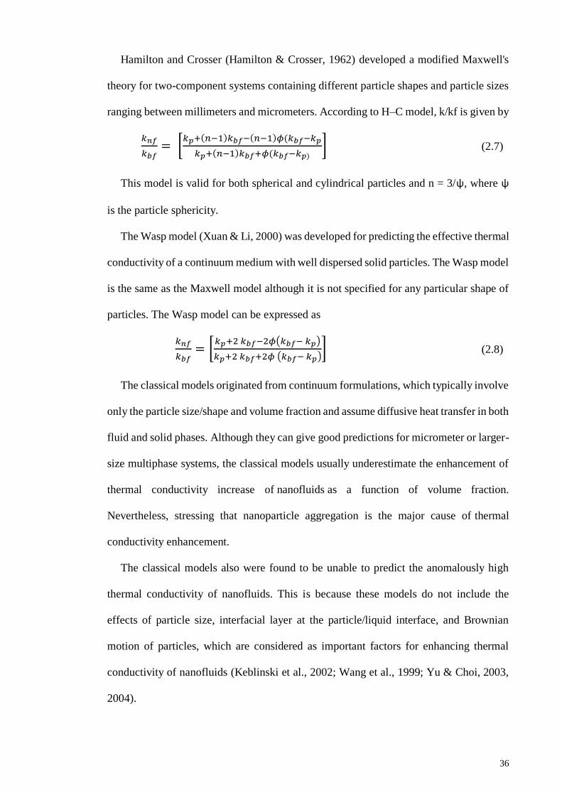
36
Hamilton and Crosser (Hamilton & Crosser, 1962) developed a modified Maxwell's
theory for two-component systems containing different particle shapes and particle sizes
ranging between millimeters and micrometers. According to H–C model, k/kf is given by
𝑘𝑛𝑓
𝑘𝑏𝑓= [
𝑘𝑝+(𝑛−1)𝑘𝑏𝑓−(𝑛−1)𝜙(𝑘𝑏𝑓−𝑘𝑝
𝑘𝑝+(𝑛−1)𝑘𝑏𝑓+𝜙(𝑘𝑏𝑓−𝑘𝑝)] (2.7)
This model is valid for both spherical and cylindrical particles and n = 3/ψ, where ψ
is the particle sphericity.
The Wasp model (Xuan & Li, 2000) was developed for predicting the effective thermal
conductivity of a continuum medium with well dispersed solid particles. The Wasp model
is the same as the Maxwell model although it is not specified for any particular shape of
particles. The Wasp model can be expressed as
𝑘𝑛𝑓
𝑘𝑏𝑓= [
𝑘𝑝+2 𝑘𝑏𝑓−2𝜙(𝑘𝑏𝑓− 𝑘𝑝)
𝑘𝑝+2 𝑘𝑏𝑓+2𝜙 (𝑘𝑏𝑓− 𝑘𝑝)] (2.8)
The classical models originated from continuum formulations, which typically involve
only the particle size/shape and volume fraction and assume diffusive heat transfer in both
fluid and solid phases. Although they can give good predictions for micrometer or larger-
size multiphase systems, the classical models usually underestimate the enhancement of
thermal conductivity increase of nanofluids as a function of volume fraction.
Nevertheless, stressing that nanoparticle aggregation is the major cause of thermal
conductivity enhancement.
The classical models also were found to be unable to predict the anomalously high
thermal conductivity of nanofluids. This is because these models do not include the
effects of particle size, interfacial layer at the particle/liquid interface, and Brownian
motion of particles, which are considered as important factors for enhancing thermal
conductivity of nanofluids (Keblinski et al., 2002; Wang et al., 1999; Yu & Choi, 2003,
2004).

37
Recently, many theoretical studies have been carried out to predict the anomalously
increased thermal conductivity of nanofluids. A detailed summary of recently developed
models for the prediction of the effective thermal conductivity of nanofluids is provided
in Table 2.2.
Table 2.2: Summary of models developed for thermal conductivity of nanofluids
i. Researchers ii. Models/equations Remarks
iii. (Wang et al.,
2003)
iv. 𝑘𝑓
𝑘𝑏𝑓=
(1−𝜙)+3𝜙 ∫𝑘𝑐𝑙(𝑟)𝑛(𝑟)
𝑘𝑐𝑙(𝑟)+2𝑘𝑏𝑓𝑑𝑟
∞°
(1−𝜙)+3𝜙 ∫𝑘𝑏𝑓𝑛(𝑟)
𝑘𝑐𝑙(𝑟)+2𝑘𝑏𝑓𝑑𝑟
∞
°
v. Based on effective
medium
approximation and
fractal theory
vi. (Xuan et al.,
2003)
vii. 𝑘𝑓
𝑘𝑏𝑓=
𝑘𝑝+2𝑘𝑏𝑓−2𝜙(𝑘𝑏𝑓−𝑘𝑝)
𝑘𝑝+2𝑘𝑏𝑓+𝜙(𝑘𝑏𝑓−𝑘𝑝)+
𝜙𝜌𝑝𝑐𝑝
2𝑘𝑏𝑓√
𝐾𝐵 𝑇
3𝜋𝑟𝑐𝜂
The first term is the
Maxwel models
(Yu & Choi,
2003)
𝑘𝑓
𝑘𝑏𝑓=
𝑘𝑝𝑐 + 2𝑘𝑏𝑓 − 2𝜙(𝑘𝑝𝑐 − 𝑘𝑏𝑓)(1 + 𝛽)3
𝑘𝑝𝑐 + 2𝑘𝑏𝑓 − 𝜙(𝑘𝑝 − 𝑘𝑏𝑓)(1 + 𝛽)3
Considered interfacial
layer when modified
Maxwell model
(Yu & Choi,
2004)
𝑘𝑓
𝑘𝑏𝑓= 1 +
𝑛𝜙𝑓𝐴
1−𝜙𝑓𝐴2 where 𝐴 =1
3∑
𝑘𝑝𝑗−𝑘𝑏𝑓
𝑘𝑝𝑗+(𝑛−1)𝑘𝑏𝑓𝑗=𝑎,𝑏,𝑐
Considered interfacial
layer when modified
Hamilton and Crosser
model
(Kumar et
al., 2004)
𝑘𝑓
𝑘𝑏𝑓= 1 + 𝑐
2𝐾𝐵𝑇
𝜋𝜂𝑑𝑝2
𝜙𝑟𝑏𝑓
𝑘𝑏𝑓(1 − 𝜙)𝑟𝑝 Based on kinetic
theory and Fourier’s
law
(Leong et al.,
2006)
𝑘𝑓
= (𝑘𝑝 − 𝑘𝑏𝑓)𝜙𝑝𝑘𝑙𝑟[2𝛾𝑙
3 − 𝛾3 + 1] + (𝑘𝑝 + 𝑘𝑙𝑟)𝛾𝑙3[𝜙𝑝𝛾3(𝑘𝑙𝑟 − 𝑘𝑏𝑓) + 𝑘𝑏𝑓]
𝛾𝑙3(𝑘𝑝 + 2𝑘𝑙𝑟) − (𝑘𝑝 − 𝑘𝑙𝑟)𝜙𝑝[𝛾𝑙
3 + 𝛾3 − 1]
Considered interfacial
layer as separate
component and for
spherical shape
particle
(Jang &
Choi, 2004)
𝑘𝑓
𝑘𝑏𝑓= 1 + 𝑐
𝑑𝑓
𝑑𝑝𝑘𝑏𝑓𝜙𝑅𝑒
2𝑑𝑝𝑃𝑟 Based on convection
and conduction heat
transport
(Xie et al.,
2005)
𝑘𝑓
𝑘𝑏𝑓= 1 + 3Θ𝜙 +
2Θ2𝜙2
1 − 𝛩𝜙
Considered the
presence of a
nanolayer
(Murshed et
al., 2008) 𝑘𝑓 =
(𝑘𝑝 − 𝑘𝑙𝑟)𝜙𝑝𝑘𝑙𝑟[𝛾𝑙2 − 𝛾2 + 1] + (𝑘𝑝 + 𝑘𝑙𝑟)𝛾𝑙
2[𝜙𝑝𝛾2(𝑘𝑙𝑟 − 𝑘𝑏𝑓) + 𝑘𝑏𝑓]
𝛾𝑙2(𝑘𝑝 + 𝑘𝑙𝑟) − (𝑘𝑝 − 𝑘𝑙𝑟)𝜙𝑝[𝛾𝑙
2 + 𝛾2 − 1]
For cylindrically
shaped particles in
base fluid
(Koo &
Kleinstreuer,
2004)
𝑘𝑓
𝑘𝑏𝑓=
𝑘𝑀𝐺
𝑘𝑏𝑓+
1
𝑘𝑏𝑓5 𝑥 104𝛽𝜙𝜌𝑝𝑐𝑝√
𝐾𝐵 𝑇
𝜌𝑝𝐷𝑓(𝑇, 𝜙)
Assumed randomly
moving nanoparticles
with surrounding
liquid motion having
unknown parameters
of β and f
(Jang &
Choi, 2004)
𝑘𝑓
𝑘𝑏𝑓= 𝑘𝑏𝑓 + (1 − 𝜙) + 𝑘𝑝𝜙 + 𝜙ℎ𝛿𝑇
Considered the
thickness liquid layer
and Brownian motion
of dispersed particles.
(Pak & Cho,
1998)
𝑘𝑓
𝑘𝑏𝑓= 1 + 7.47𝜙
Assumed that k
enhancement is due to
the suspended particle

38
(Gupte et al.,
1995)
𝑘𝑓 = 𝑘𝑏𝑓(0.0556 𝑃𝑒 + 0.1649 𝑃𝑒2 − 0.0391 𝑃𝑒
3 + 0.0034 𝑃𝑒4)
Considered the effect
of translational
motion of
nanoparticle
(Evans et al.,
2008)
𝑘𝑓
𝑘𝑏𝑓= 1 + 𝜙𝑝
𝑘𝑝
3𝑘1
Considered
aggregation and
interfacial layer of the
particle thermal
conductivity
(Timofeeva
et al., 2007)
𝑘𝑓
𝑘𝑏𝑓= 1 + 3𝜙
Considered the
agglomeration of the
nanoparticle
2.6.1.2 Experimental Investigation
Most of the investigation of nanoparticles as heat transfer application is the property
of thermal conductivity. Due to their higher thermal conductivity of particles compared
to base fluids, it is believed that suspended nanoparticle in fluids will enhance thermal
conductivity of fluids. For magnetic fluids, investigation of thermal conductivity
conducted in the absence and presence of magnetic fields effect.
Experimental investigations on the thermal conductivity of magnetic nanofluids in the
absence of magnetic fields show that the increase of thermal conductivity is mainly
affected by several parameters. These parameters are volume fraction of magnetic
nanoparticles, particle size/particle size distribution, the chemical composition of
magnetic nanoparticles, temperature, particle coating layer.
Many investigators show that the thermal conductivity of magnetic fluids increase with
the increasing of particles fraction and temperature. Abareshi measured the thermal
conductivity of a water based magnetite nanofluids as a function of the particle volume
fraction at different temperatures. The thermal conductivity enhanced with the increase
of the particle volume fraction and temperature. The largest thermal conductivity ratio
observed was 11.5% at a particle volume fraction of 3% at 40 °C (Abareshi et al., 2010).
Li et al. (2005) investigated the effects of particle volume fraction, surfactants and the
magnetic field on the transport properties of water based Fe magnetic nanofluids. They
observed a thermal conductivity enhancement of magnetic nanofluids with the increase

39
of particle volume fraction with and without applied magnetic fields. Their results also
revealed that the viscosity of magnetic nanofluids increased with the increase of particle
volume fraction and the surfactant.
Yu et al. (2010) investigated the effects of the particle volume fraction on the thermal
conductivity of a kerosene-based magnetite nanofluid prepared via a phase-transfer
method. The results describe that the thermal conductivity ratios increased linearly with
the increase of volume fraction and temperature, and the value was up to 34.0 % at 1 vol
%. The measurement was conducted in the different temperature range from 10 to 60 oC
in order to investigate the effect of temperature on thermal conductivity. The results
revealed that the absolute thermal conductivity improved with increasing temperature.
While the thermal conductivity ratio was nearly constant, and the thermal conductivities
of the magnetic nanofluids tracked those of the carrier fluid.
Philip et al. (2007) conducted a work on thermal conductivity of magnetic nanofluids
prepared via the dispersion of magnetite nanoparticles in water, ethylene glycol, and
kerosene as carrier fluids, respectively. Their results revealed that the thermal
conductivity ratio increased with the increase of particle volume fraction. (Philip et al.,
2007) (Philip et al., 2007) (Philip et al., 2007) (Philip et al., 2007) (Philip et al., 2007)
(Philip et al., 2007) (Philip et al., 2007) (Philip et al., 2007) (Philip et al., 2007)
The thermal conductivity enhancement of Fe3O4/water nanofluids depends on the
particle volume concentration and temperature. Thermal conductivities are higher at
higher volume concentrations (Sundar et al., 2013).
Recent work on the control of the thermal conductivity of magnetic nanofluids has
received particular interest because the “anomalous” thermal conductivity observed under
the influence of an external magnetic field. The thermal conductivity of magnetic
nanofluids can be affected by the orientation, and the intensity of the presence of the
applied magnetic field. The same techniques as those used in without magnetic fields are

40
conducted to measure thermal conductivity in the presence of magnetic field and usually
performed at room temperature. The magnetic field is created by either electromagnets or
permanent magnets.
Krichler & Odenbach (2013) investigated the influence of magnetically driven
structure formation on heat flux in magnetic nanofluids. They conducted the
measurements of thermal conductivity in the different of external magnetic field. They
developed an improved measuring device based on the plane heat source instead of the
standard hot wire method was used to enable both parallel and perpendicular orientations
of a magnetic field and heat flux. Thermal conductivity measurements were conducted
on the variation of strength and direction of an external magnetic field about heat flux. It
was concluded that the results showed qualitative consistency with theoretical predictions
for both orientations.
Li et al. (2005) also reported on the influence of magnetic field strength and direction
on the transport properties of magnetite nanofluids. Their results show that an external
magnetic field had outstanding effects on the both thermal conductivity and viscosity of
the magnetite nanofluids. Little change in the thermal conductivity of the magnetite
nanofluids was found in the magnetic field perpendicular to the temperature gradient,
irrespective of the applied magnetic field strength and the volume fraction of particles.
The thermal conductivity of the magnetite nanofluids increased with the increase of
strength of magnetic field in which parallel to the temperature gradient. The reason for
this enhancement was the change of microstructures induced by the external magnetic
field in the magnetite nanofluids. They further clarified that when the magnetic field was
parallel to the temperature gradient, the formed particle chains give more bridges for
energy transport inside the magnetite nanofluids. This phenomenon occurred along the
direction of temperature gradient and enhanced the thermal process in the magnetite
nanofluids. It was revealed that the viscosity firstly increased with the magnetic field and

41
finally approached a constant as the magnetization of the magnetic fluid achieved a
saturation state. This behavior was also explained by the presence of chain-like structures
in magnetic nanofluids with respect to the influence of magnetic fields.
Philip et al. (2007;2008) reported a remarkable enhancement of the thermal
conductivity of magnetite-based nanofluids under the effect of magnetic fields along the
direction of heat flow. The enhancement of thermal conductivity was within the predicted
value for parallel mode conduction. The decrease in thermal conductivity observed after
the critical value of the magnetic field was explained by the “zippering” of chains. They
claimed that the cluster morphology and distribution of both could have impacts on
thermal conductivity enhancement. These behaviors support the transfer of heat through
the particles. A magnetically polarizable nanofluid (magnetic nanofluid) could be used
as a reversible switchable thermal fluid, such as insulation to high thermal conducting
fluid and vice versa, by changing the magnetic fields.
Wensel et al. (2008) investigated the thermal conductivity of nanofluids with metal
oxides nanoparticles (Fe3O4 and MgO) and carbon nanotubes in the presence of magnetic
field. They observed that thermal conductivity increased by up to 10% at a low particle
weight fraction of 0.02 wt%. This phenomenon is because of the aggregation of metal
oxide on the surface of the nanotube by electrostatic attraction and the formation of chain
structure along the nanotube. It was proposed that the investigated nanofluids could be
used for coolant applications since their viscosity was similar to that of water.
Nkurikiyimfura et al. (2011) investigated the effects of particle size and particle
volume fraction on the thermal conductivity enhancement of an engine oil based
magnetite nanofluids in a magnetic field. The results revealed that the thermal
conductivity increased with the increase of particle volume fraction for smaller magnetite
particles. Besides, the thermal conductivity enhancement corresponding to a magnetic
field parallel to temperature gradient. They analyzed that the increase of thermal
42
conductivity ratio was due to the chain-like structures formed in magnetic nanofluids
under the effect of magnetic field. The increased thermal conductivity observed for the
smaller particles was justified by the superparamagnetic behavior of the less particulate
matter and their influence on the aggregates formation. The magnetic field parallel to
temperature gradient exhibited a positive effect on the thermal conductivity of the
magnetic nanofluids. However, a high magnetic field set back thermophysical properties
such as rheological and thermal conductivity itself (Nkurikiyimfura et al., 2011; Philip et
al., 2007). Because of the undesirable clumping and zippering of chains under the effect
of high magnetic fields. This restriction calls for the simultaneous treatment of thermal
conductivity enhancement with other transport properties, especially, the viscosity (η).
Once the thermal conductivity and magnetoviscous effects were taken into account, the
improvement could be considered by a ratio of the thermal conductivity to the viscosity
(Nkurikiyimfura et al., 2011).
Gavili et al. (2012) conducted an experimental investigation on the thermal
conductivity of water-based magnetite nanofluids under the magnetic field using the
Helmholtz coils. The magnetic field strength was controlled by an electric current. The
saturation time and the reversibility of thermal conductivity were also observed after the
magnetic field was turned off. The results revealed that the thermal conductivity increased
more than 200% for magnetite nanofluids with 5.0% volume fraction with an average
diameter of 10 nm. Furthermore, the variation of thermal conductivity with temperature
was also shown.
2.6.2 Viscosity
Viscosity is the friction between neighboring particles in a fluid that are moving at
different velocities. When the fluid is forced through a tube, the fluid moves faster near
the axis and very slowly near the walls. Therefore, some stress (such as a pressure
difference between the two ends of the tube) is required to overcome the friction between

43
layers and keep the fluid moving. For the same velocity pattern, the stress required is
proportional to the fluid's viscosity. A liquid's viscosity depends on the size and shape of
its particles and the attractions between the particles.
Viscosity describes the internal resistance of a fluid to flow, and it is an important
property for all thermal applications involving fluids (Nguyen et al., 2007b). The pumping
power is related to the viscosity of a liquid. In laminar flow, the pressure drop is directly
proportional to the viscosity. Furthermore, convective heat transfer coefficient is
influenced by viscosity. Hence, viscosity is as important as thermal conductivity in
engineering systems involving fluid flow (Kole & Dey, 2010).
Measurement of viscosity is conducted by various types of viscometer and rheometers.
A rheometer is used for those liquids that cannot be defined by a single value of viscosity
and, therefore, need more parameters to be set and measured than is the case for a
viscometer. Temperature control of the liquid is an essential parameter to obtain precise
measurements, particularly in materials like lubricants. One of the most common
apparatus for measuring kinematic viscosity is the glass capillary viscometer.
2.6.2.1 Theoretical Formula
There are some existing theoretical formulas to estimate the particle suspension
viscosities depending on the size and concentration of the solid particles. Some models
exist that describe the relative viscosity as a function of volume fraction ϕ of solid
particles. Among them, equation suggested by Einstein could be labeled the pioneer one,
and most of other derivations have been established from this relation (Einstein, 1906).
The assumptions are based on the linear viscous fluid containing dilute, suspended,
spherical particles and low particle volume fractions (ϕ < 0.02). The suggested formula
is represented by equation 2.9 as follows:
𝜇 = 𝜇𝑏𝑓(1 + 2.5 𝜙) (2.9)

44
where µ is the viscosity of suspension; µbf is the viscosity of the base fluid, and ϕ is the
volume fraction of a particle in a base fluid. This equation is a linear increase of the
suspension viscosity with increasing solid volume concentration. The Einstein model for
nanofluids is according to the assumption of a Newtonian fluid containing suspensions of
spherical nanoparticles. It does not take into account temperature dependence and, in
general, the viscosity of liquids is strongly dependent on the temperature. Einstein
considered non-interacting suspensions. Some factors have been identified as the
limitations of this formula as the particle concentrations may not be so small. The
structure and the interaction of the particles within the continuous phase may also affect
the viscosity of the mixture.
Brinkman extended Einstein’s formula to be used with moderate particle
concentrations, taking into account the effect of the addition of one solute-molecule to an
existing solution, which is considered as a continuous medium. And this correlation has
more acceptances among the researchers (Brinkman, 1952). For particle concentrations
less than 4%, the expression is represented by equation 2.10.
𝜇 = 𝜇𝑛𝑓 (1 − 𝜙)2.5 (2.10)
Lundgren (Lundgren, 1972) proposed the following equation under the form of a
Taylor series in ϕ. The equation is represented by equation 2.11.
𝜇 = 𝜇𝑏𝑓(1 + 2.5 𝜙 + 25
4 𝜙2 + 𝑓(𝜙3) (2.11)
Considering the effect due to the Brownian motion of particles on the bulk stress of an
approximately isotropic suspension of rigid and spherical particles; (Batchelor, 1977)
proposed the equation as expressed by equation 2.12.
𝜇 = 𝜇𝑏𝑓(1 + 2.5 𝜙 + 6.5 𝜙2) (2.12)
From the above two relations, if a second or higher order of ϕ are ignored, then these
formulas will be the same as Einstein’s formula. Eq. (2.12) has been validated for a
45
particle volume fraction up to ϕ ≤ 0.1 where the motion of the single particle and pair-
particle interactions is dominant. Batchelor considered the interaction of pair-particles.
There are many of other theoretical formulas developed by researchers for higher
particle volume concentration which have not describe here.
2.6.2.2 Experimental Investigation
Due to their unique properties, magnetic nanoparticles have been attracted many
researchers to investigate these smart materials. Most of the investigations available in
the literature on the viscosity of nanofluids, regarding the effect of volume fraction agree
upon the fact that the viscosity of nanofluids increases with increasing the particle volume
fractions. This phenomenon also occurs in magnetic nanofluids.
Several authors reported that in the absence of a magnetic field, the viscosity of a fluid
with dispersing magnetic nanoparticles is similar to other types of nanofluids. The
viscosity increases proportionally with the volume fraction (Mahbubul et al., 2012;
Sundar et al., 2013).
The influence of volume fraction and temperature on viscosity of Fe3O4-water
nanofluids have been investigated by (Sundar et al., 2013). The results show that Fe3O4-
water magnetic nanofluid exhibited Newtonian behavior. The viscosity of nanofluids
increases with an increase in particle volume concentration and decreases with a rise in
temperature.
In a strong magnetic field, the magnetic fluids form chains directed to magnetic fields
that are zippered and clumped together. It will block the motion of the particle and
significantly reduce the flow ability of the fluid, hence increase the viscosity of a
condensed magnetic fluids (Genc & Derin, 2014). Many works supported by many
workers that the viscosity of magnetic fluids would increase under the existence of a
magnetic field (Nowak et al., 2014; Patel et al., 2003). Patel also used a horizontal
viscometer to study the effective viscosity as a function of external magnetic field,

46
parallel, perpendicular, and in other angular directions to the flow. The results also
showed that the orientation of the magnetic field played affects greatly the viscosity of
magnetic fluids. The viscosity was magnified up to 200% when the magnetic field was
shifted from perpendicular to parallel to the flow direction. They also investigated the
dependence of viscosity of magnetic fluids on the intensity of the magnetic field and the
volume fraction of a particle in the experiment. They found that introducing either a
strong field or decrease the volume fraction resulted in the increase of viscosity.
Moeen investigated the rheological properties of magnetic fluids by using a standard
rotating rheometer with a variable magnetic field. The results suggested the presence of
a remarkable magneto-viscous effect at a low shear rate. The increase in viscosity is due
to the magnetic torques spreading though the suspensions which tries to align the particles
magnetic moments with the magnetic field direction (Moeen et al., 2012).
Li et al. (2005) study the effect of magnetic particle and surfactant concentrations and
magnetic strength on the viscosity of Fe3O4-water magnetic fluids using capillary tube
viscometer. The results show that the viscosity of magnetic fluids increases with the
magnetic particle and surfactant concentrations. The magnetic field strength plays
significant roles in affecting the viscosity of magnetic fluids. The viscosity increases with
the strength of magnetic field.
2.6.3 Electrical Conductivity
Electrical conductivity of a nanofluid is related to the ability of charged particles (ions)
in the suspension to carry the charges (electrons) towards respective electrodes when an
electric potential is applied. In nanofluids, the nanoparticles dispersed in a base fluid get
charged due to the formation of electrical double layer around the particle surface. These
nanoparticles along with the EDL move towards oppositely charged electrode when a
potential is applied. This EDL formation depends on the surface charge, size, and volume

47
fraction of the particles and ionic concentration in the base fluid. Thus, the electrophoretic
mobility of charged particles determines the electrical conductivity of a nanofluid.
The electrical conductivity of a suspension depends on the background electrolyte and
particle size, charge, and volume fraction (Posner, 2009). When nanoparticles dispersed
in fluid, these particles gain surface charge due to the protonation or deprotonation of a
surface group such as a hydroxyl ligand (-OH) (Lee et al., 2006). This surface charge,
which can be adjusted in electrolyte solutions by altering the pH of the suspension (Li et
al., 2008; Lee, 2007) or chemically treating the particle surface (Lee, 2007), causes an
electrical double layer EDL of counter-ions to form near the particle surface. For bulk
suspensions that are salt-free, the only ions present are those from the charging process
of the particles, which are counter-ions formed at the fluid-particle interface. For salt-free
suspensions, the effective electrical conductivity is typically increased upon the
suspension of particles since the ionic conductivity in the EDL is generally larger than
that of the bulk solution (Posner, 2009).
In fact, the observed enhancement in electrical conductivity of the suspension with
respect to the base fluid is a consequence of net charge effect of the solid particle and the
pertinent EDL interactions (Hunter, 2013; Lyklema, 2005). When particles are suspended
in a polar liquid, electric charges develop on their surfaces. Ions of charge opposite to that
of the particle surface are attracted, causing the development of a charged diffuse layer
surrounding the particle. This layer is known as electrical double layer (Hunter, 2013) and
is commonly characterized by a parameter κ − 1 (Debye length).
Apart of the physical properties of fluid as well as conductivity of particles and fluids,
the effective electrical conductivity of colloidal nanosuspensions in a liquid exhibits a
complex dependence on the electrical double layer, EDL characteristics, volume fraction,
ionic concentrations, and other physicochemical properties. When the ionic strength of
the solution is very low, the number of ions in solution is insufficient to compensate the

48
electric charges, and hence the net electric charge density is high on particle surfaces. The
surface charge of the particles, together with ion-cloud that constitutes the EDL, actively
contributes for the enhancement in conduction mechanisms through the suspension. In
addition, the presence of uniformly dispersed nanoparticles is characterized with reduced
equivalent particulate masses, leading to increase electrophoretic mobility, which
consequently increases the effective electrical conductivity of the nanofluids. With an
increase in particle volume fraction, the availability of conducting path-ways increases in
the solution, which in turn increases the overall electrical conductivity of the solution.
Though the electrical conductivity of the nanoparticles and the base fluid are in the
same order, the electrical conductivity of the nanofluids is much higher than that of the
base fluid. This reveals that the electrical conductivity of the nanofluid is not only related
to the physical properties of the base fluid and nanoparticles but is also strongly affected
by other factors such as the electrochemical properties, electrical double layers, particle
size, and aggregation. The higher the temperature is, the greater the electrical conductivity
will be.
2.6.3.1 Theoretical models
The Maxwell model was the first model developed to determine the effective electrical
or thermal conductivity of liquid–solid suspensions (Maxwell, 1954). This model is
applicable to statistically homogeneous and low volume fraction liquid–solid suspensions
with randomly dispersed, uniformly sized and noninteracting spherical particles.
The electrical conductivity of nanofluids in the Maxwell model, σM, as a function of
volume fraction, ϕ, is given equation 2.13.
𝜎𝑀
𝜎𝑜= 1 +
3(𝛼−1)
(𝛼+2)−(𝛼−1)𝜙 (2.13)
where σ₀ is the electrical conductivity of base fluids, and 𝛼 =𝜎𝑝
𝜎𝑜 is the conductivity ratio
of the nanoparticle, σp, to the base fluids. This model does not include the particle surface

49
charge effects, and motion of particles, which are important factors for the enhancement
of the electrical conductivity of nanofluids.
According to the theory of colloid and surface chemistry, there is an electrical double
layer around each particle surface. The surface charge of the particles, together with ion
cloud that constitutes the EDL, would contribute to the enhancement in conduction
through the electrophoretic transactions. Generally, the particles are positively charged
when their dielectric constant is larger than that of the base fluid. And in turn, the particles
will be negatively charged. The nanoparticle has a Zeta potential Uo relative to the base
liquid. When an electrical field is applied, the charged particles will move towards the
electrode and thus form the electrophoretic conductivity. That is to say that the
nanoparticles are electric current carriers in the fluid.
The electron attachment on the particle can be expressed as:
𝑞 = 4 𝜋휀𝑟휀𝑜𝑟 𝑈𝑜 (2.14)
Considering that the particle has uniform velocity under the joint function of electric
force and viscous force, the electrophoretic conductivity can be expressed as:
𝜎𝐸 =8𝜋𝑛𝑜𝜀𝑟
2𝜀𝑜2𝑈𝑜
2
3𝜂 (2.15)
where no is the number of particles per unit volume, η is the dynamic viscosity of the
liquid, ε₀ is the dielectric constant of the vacuum, and εr is the relatively dielectric constant
of nanoparticles. If the no, εr, Uo, and r remain unchanged, the value of σEη is a constant.
The relationship indicates that though the electrical conductivity and viscosity of the base
fluids change with temperature, the product of σE and η will remain constant in the
nanofluids. This relationship is called Walden law (Bailar Jr & Auten, 1934). Hence, no
can be expressed as.
𝑛𝑜 = 1𝜙
4
3 𝜋𝑟3
= 3𝜙
4𝜋𝑟3 (2.16)
Substituting this result into eq. (2.15) gives:

50
𝜎𝐸 =2𝜙𝜀𝑟
2𝜀𝑜2𝑈𝑜
2
𝜂𝑟2 (2.17)
On the other hand, the relationship of dynamic viscosity and kinematic viscosity is
𝜂 = 𝜌𝜐 (2.18)
In nanofluids, both the dynamic viscosity and zeta potential will be affected by the
fluctuation of the volumetric fraction of nanofluid. The variation of dynamic viscosity
with respect to the volumetric fraction of nanofluid is given by Eq. (2.19) when
considering the interaction of particles. When the volume fraction of nanofluid is lower
than 10 %, η can be described as (Shen et al., 2012).
𝜂 = 𝜂𝑓 (1 + 25𝜙 + 625𝜙2) (2.19)
where ηf is the dynamic viscosity of pure base fluid.
In fluid mechanics, the viscosity varies with pressure and temperature. Since the
pressure has a very small influence on the viscosity, it is only considering the effect of
temperature. The relationship between viscosity and temperature can be expressed as
(Dong et al., 2013).
𝜂 = 𝜂₀ 𝑒−𝜆(𝑇−𝑇𝑜) (2.20)
where η₀ is the dynamic viscosity of the nanofluid at temperature and λ is the
decreasing rate of the viscosity when the temperature is increasing, namely, the viscosity
index of the fluid.
The electrophoresis conductivity is obtained by substituting eqs. (2.18), (2.19), (2.20)
into (2.17)
𝜎𝐸 = 2𝜙𝜀𝑟
2𝜀𝑜2𝑈𝑜
2
𝜌𝜐(1+25𝜙+625𝜙2)𝑟2 𝑒𝜆(𝑇−𝑇𝑜) (2.21)
In addition to the electrophoresis of the nanoparticles in fluid, the Brownian motion of
the suspended nanoparticles is also suggested to be responsible for the extra electrical
conductivity enhancement. Considering nanoparticles randomly dispersed in the fluid, the
Brownian motion of the nanoparticles is similar with the molecular in fluid with a mean

51
kinetic energy of 3
2 kT. Assuming the particles are spherical, in the view of molecular
motion and by Boltzmann distribution law, the average displacement of a nanoparticle in
time t can be expressed as (Dobnikar et al., 2004).
𝑥 = (𝑅𝑇
𝐿
𝑡
3𝜋𝜂𝑟)1/2 (2.22)
here T is the temperature in Kelvin, L is the Avogadroʼs constant, R is the thermodynamic
constant. η is the dynamic viscosity of the nanofluid and r is the average radius of the
monodispersed nanoparticles in fluid. Then the electrical conductivity of the nanofluid
caused by the Brownian motion can be inferred as:
𝜎𝐵 = 3𝜙𝜀𝑟𝜀𝑜 𝑈𝑜
𝑟3/2 (𝑅𝑇
𝐿
𝑒𝜆(𝑇−𝑇𝑜)
3𝜋𝜌𝜐(1+25𝜙+625𝜙2))1/2 (2.23)
Finally, considering that in nanofluid 𝜎𝑝
𝜎𝑜 >>1, the total electric conductivity is the sum
of the Maxwell conductivity and dynamic electrical conductivity caused by the
electrophoresis and Brownian motion of the nanoparticles. Consequently, the electric
conductivity model can be defined as:
𝜎 = 𝜎𝑀 + 𝜎𝐸 + 𝜎𝐵
= 𝜎𝑜(𝑇)(1 + 3𝜙) + 2𝜙휀𝑟2휀𝑜
2𝑈𝑜2
𝜌𝜐(1+25𝜙+625𝜙2)𝑟2
𝑒𝜆(𝑇−𝑇𝑜)
+ 3𝜙𝜀𝑟𝜀𝑜 𝑈𝑜
𝑟3/2 (𝑅𝑇
𝐿
𝑒𝜆(𝑇−𝑇𝑜)
3𝜋𝜌𝜐(1+25𝜙+625𝜙2))1/2 (2.24)
2.6.3.2 Experimental investigations
The major focus of the research work, so far, has been on the estimation of thermo-
physical properties, primarily on the effective thermal conductivity. Despite the vast
scientific and technological importance of electrical conductivity characteristics of
nanoparticle suspensions, studies concerning the issue of the effective electrical
conductivities of nano-fluids have been largely ignored. In addition, there is very few data
published on the electrical properties of nanofluids. On the other hand, among the
52
transport properties, electrical conductivity might bring information on the state of
dispersion and stability of the particulate suspension.
Despite the vast scientific and technological importance of electrical conductivity of
nanofluids, studies concerning this issue have been largely ignored. Lack of electrical
conductivity data is available in the literature with only a few papers about the
measurement of electrical conductivity of nanofluids. Ganguly (Ganguly et al., 2009)
investigated the effective electrical conductivity of aluminum oxide nanofluids as a
function of particle volume fraction and temperature. The results indicate that increase of
electrical conductivity of aluminum oxide with increasing of particle volume fraction and
temperature. Electrical and thermal conductivities of gold nanofluids have been studied
(Fang & Zhang, 2005). Few investigations dealt with numerical and analytical studies on
electrical conductivity of concentrated and dilute colloidal suspensions (Cruz et al., 2005;
O'brien, 1981).
A linear rise in electrical conductivity of TiO2 suspensions with particle fraction was
observed for low ionic strength and no significant impact for high ionic concentrations
by Luis and Biswas (Modesto-Lopez & Biswas, 2010). Thermal and electrical
conductivities of suspensions of multiwalled carbon nanotubes
(MWCNT) in water were measured as a function of temperature, nanotube weight
content, and nanotube length (Glory et al., 2008). The synthesis of highly stable exfoliated
graphene based nanofluids with water and ethylene glycol as base fluids without any
surfactant and the subsequent studies on their thermal and electrical conductivities (Baby
& Ramaprabhu, 2010).
Sarojini et al. (2013) conducted an experimental evaluation of electrical conductivity
of ceramic and metallic nanofluids with a different volume fraction in water and ethylene
glycol base fluids. The results show that the electrical conductivity of nanofluids increases
with the increasing particle volume fraction in both base fluids. Electrical conductivity of

53
magnetite nanofluids were investigated by Bagheli et al. (2015) at different volume
fractions and temperatures. The result indicated considerable enhancement of electrical
conductivity of magnetite nanofluids with increase of volume fraction and temperature.
Recently, Zakaria et al. (2015) investigates the electrical conductivity of Al2O3 nanofluids
in water-ethylene glycol mixture. The finding shows that electrical conductivity decreases
as the ethylene glycol increased. However, no investigation of electrical conductivity has
been carried out for maghemite nanofluids.
Previous studies also elucidated that the Maxwell model underestimated the electrical
conductivity enhancement in nanofluid. This is due to the fact that the electrical
conductivity is not only associated with the physical properties of nanofluid but also
relates to some other physicochemical properties, such as the shape and size of the
nanoparticles, agglomeration, the EDL, the electrophoresis, and the Brownian motion of
nanoparticles (Dong et al., 2013; Ganguly et al., 2009; Gao et al., 2007; Minea & Luciu,
2012; Shen et al., 2012).
Several researchers have measured large increases in the electrical conductivity of
nanofluids compared to the base fluid as the volume fraction (Cruz et al., 2005; Fang &
Zhang, 2005; Ganguly et al., 2009; Lisunova et al., 2006; Wong & Bhshkar, 2006) and
temperature (Ganguly et al., 2009) are increased.
54
METHODOLOGY
This chapter describes the methodology and procedures of the synthesis,
characterization, and thermophysical properties of maghemite nanofluids with and
without magnetic fields effect. There are three main stages of the experiment. Figure 3.1
shows all steps and procedures of this research.
3.1 Materials
The first stage of the research is the synthesis of maghemite nanoparticles using
chemical co-precipitation method. The raw materials for synthesis of maghemite
nanoparticles were ferric chloride hexahydrate (Sigma-Aldrich), ferrous chloride
tetrahydrate (Sigma-Aldrich), ammonium hydroxide 28 % (Merck), nitric acid 65 %
(Merck), hydrochloric acid 37 % (Ajax), ferric nitrate nonahydrate (Sigma-Aldrich), and
deionized water.
The second stage of this study involved the preparation of maghemite nanofluids and
their stability characterizations. The raw materials used for this phase are sodium
hydroxide (Merck), hydrochloric acid (Sigma-Aldrich) and deionized water.
The third stage of the research is the characterization of thermophysical properties of
maghemite nanofluids. The raw materials used at this point are maghemite nanofluids and
deionized water.
Deionized water with resistivity around 15 MΩ/cm was obtained using ELGA ultra
analytic deionized and was used for the preparation of solution throughout the whole
experiment. All chemicals were analytical grade and used as received without further
purification.

55
Phase and crystal structure
Morphology analysis
Thermal Stability
Magnetization analysis sample with the smallest size
Proceed to stage II
Zeta potential analysis
Dynamic light scattering analysis
Sample with highest stability
Proceed to stage III
Thermal conductivity
Viscosity
Electrical conductivity
Figure 3.1: Flowchart of research methodology
3.2 Synthesis of Maghemite Nanoparticles
Maghemite nanoparticle was synthesized by a chemical co-precipitation method. In
this method, ferric chloride solution (stabilized with a few drops of hydrochloric acid)
and ferrous chloride solution with molar ratio 2:1 were mixed. Then ammonium
hydroxide solution was added to the solution with vigorous stirring for 20 minutes at
room temperature. A black precipitate produced was separated from solution using a
Selection of Materials
Stage II
Preparation of maghemite
nanofluids
Stage III
Physical properties of maghemite
nanofluids with and without magnetic
fields effect
Stage I
Synthesis of maghemite
nanoparticles via chemical co-
precipitation method
Characterization of
maghemite nanoparticles
Characterization of maghemite
nanofluids stability
Physical properties
End

56
Gmagnet and washed several times by stirring for 5 minutes in deionized water. The
precipitate is then stirred for 10 minutes in the nitric acid solution. The precipitate
obtained was separated and washed several times and then oxidized to maghemite at 90
oC for 30 minutes using ferric nitrate solution. Brown precipitate was isolated from
solution and then washed thoroughly with deionized water. Powder samples were
obtained by drying the suspension in the oven at a slightly elevated temperature. The flow
chart of the process is shown in Fig. 3.2. Characterization of maghemite nanoparticles
conducted by several methods including X-Ray Diffraction (XRD), Transmission
Electron Spectroscopy (TEM), Alternating Gradient magnetometer (AGM),
Thermogravimetry Analysis (TGA), Dynamic Light Scattering (DLS) and Zeta Potential
Analysis.
NH4OH
+
.
Fe(NO3)3
Figure 3.2: Schematic of synthesis of maghemite nanoparticles
3.3 Preparation of Maghemite Nanofluids
The stability analysis was performed at various pHs at certain maghemite
nanoparticles volume fraction by adding sodium hydroxide and hydrochloric acid to alter
the pH of solutions. The pH of the solution was measured by a pH meter. The effect of
time on the stability of maghemite nanofluids were measured at the different time of
FeCl3 FeCl2 FeCl
3
HNO3
Drying
Characterization

57
storage. The characterization of maghemite nanofluids was conducted by dynamic light
scattering and zeta potential analysis at 2, 4, and 8 months of storage.
3.4 Thermophysical properties Measurement
3.4.1 Preparation of Maghemite Nanofluids
Maghemite nanoparticles were synthesized using a chemical co-precipitation method
(Nurdin et al., 2014). Maghemite nanofluids were prepared by dilution of a known
concentration of a stock solution in deionized water at a different percent of the particle
volume fraction of 0.1, 0.2, 0.3, 0.4, 0.5, and 0.6 %.
The concentration of the nanofluids in percent volume fraction can be estimated by
Eq. (3.1).
ϕ =
𝑚𝑝
𝜌𝑝𝑚𝑝
𝜌𝑝+
𝑚𝑓
𝜌𝑓
x 100 % (3.1)
where: ϕ : particle volume fraction
𝑚𝑝 : mass of nanoparticles
𝜌𝑝 : density of nanoparticles
𝑚𝑓 : mass of base fluids
𝜌𝑝 : density of base fluids
3.4.2 Procedure
Thermophysical properties of maghemite nanofluids were studied at various
temperature and nanoparticle volume fractions, without and with using external magnetic
fields. The suspensions placed in a glass jacketed vessel in which temperature keep
constant with a Refrigerated JEIO Tech temperature control circulator. Different
magnetic fields strengths were provided by using a pair of an electromagnet which was
measured by a magnetometer. Thermophysical properties measured were thermal
conductivity, viscosity, and electrical conductivity. Measurements conducted at various

58
3
parameters including the effect of temperature, the effect of the particle volume fraction,
and effect magnetic fields strength. Schematic of the experimental set up are shown in
Figs. 3.3, 3.4, and 3.5, respectively.
viii.
ix.
x.
xi.
xii.
Figure 3.3: Schematic of experimental set up for thermal conductivity measurement
xiii.
xiv.
Figure 3.4: Schematic of experimental set up for viscosity measurement
Remarks:
1. Temperature control circulator 5. Sensor
2. Electromagnetic coil 6. Power supply
3. Jacketed beaker glass 7. Thermal conductivity meter
4. Sample
Remarks:
1. Temperature control circulator 4. Sample
2. Electromagnetic coil 5. Glass capillary viscometer
3. Jacketed beaker glass 6. Power supply
1 2 4
5
7 6
2
1 2 3 4
6
2
5

59
xv.
Figure 3.5: Schematic of experimental set up for electrical conductivity measurement
3.4.3 Measurement
Thermal conductivity measurements were conducted by KD2 pro thermal property
analyzer equipment by Decagon Devices Company, USA, which is based on the transient
hot wire method. The KD2 Pro consists of a handheld controller and sensors that should
be inserted into the medium. The single-needle sensor with 1.3 mm diameter and 60 mm
length was used (KS-1). The sensor integrates with its interior a heating element and a
thermo-resistor, and it is connected to a microprocessor for controlling and conducting
the measurements. The measurements were performed using 30 ml sample in a cylindrical
glass tube bottle. The needle probe inserted in the sample bottle, then placed and exposed
to the water jacketed vessel that the temperature kept constant with a JEO circulating and
refrigerating water bath. The samples were allowed in the bath for 30 minutes to get
desired temperature. The measurements were conducted at a different temperature,
particle volume fraction, and magnetic fields strength. Prior to measurement, the meter
was calibrated using the buffer solutions of known thermal conductivities. Moreover, the
Remarks:
1. Temperature control circulator 5. Sensor
2. Electromagnetic coil 6. Power supply
3. Jacketed beaker glass 7. Conductivity meter
4. Sample
1 2 3 4
5 6
7
2
60
measurement of thermal conductivity of water were compared with the thermal
conductivity value of water in the literature. The measured value of thermal conductivity
value of water was 0.595 W/mK at 20 oC compared to 0.598 W/mK at 20 oC (Haynes,
2013). Thermal conductivity data were recorded five times with an interval of 15 minutes
at each parameter measurement. The average of data measurements was reported.
The viscosity of the maghemite nanofluids was measured by calibrated glass capillary
viscometer as shown in Fig. 3.6. The maghemite nanofluids sample of 7 mL charged into
the viscometer from L tube. Place the viscometer into the holder, and insert it into the
constant temperature bath and turn the instrument to its normal vertical position. Allow
about 10 minutes for the sample to get to the bath temperature desired. Apply suction to
N tube in order to draw sample slightly above E mark. To measure the efflux time, let the
liquid sample run freely down past F mark. Measuring the time for the meniscus to pass
from E mark to F mark. Calculate the kinematic viscosity in mm2/s (cSt) of the sample
by multiplying the efflux time in seconds by the viscometer constant. The measurements
were recorded five times at each parameter measurement. The average of data
measurements was reported.
Electrical conductivity was measured by a 4-cell conductivity electrode meter (Eutech
instrument PC 2700) with inbuilt automatic temperature compensation. Prior to
measurement, the meter was calibrated using the buffer solutions of known electrical
conductivities. Measurements were performed in 30 ml of the sample in a cylindrical
glass tube with the conductivity probe immersed in it. Samples were placed and exposed
to water jacketed vessel. The temperature kept constant with a JEO circulating and
refrigerating water bath, and allowed in the bath for 30 minutes to get desired temperature.
Measurements were conducted at different temperature and particle volume fractions and
repeated five times for each parameter.

61
Figure 3.6: Schematic of calibrated glass capillary viscometer
(https://www.cannoninstrument.com/Image/GetDocument/437?language=en)
3.5 Characterization Technique
In this section, several characterization techniques performed to characterize the
samples have been explained in term of their theory, principles and sample preparations.
3.5.1 X-Ray Diffraction (XRD)
X-Ray powder diffraction (XRD) is one of the most powerful techniques for
qualitative and quantitative analysis of crystalline compounds such as a pattern-fitting
procedure for quantitative analysis of crystalline pharmaceuticals in solid dosage and a
quantitative analysis of binary system of crystalline pharmaceuticals in tablets (Takehira
et al., 2010; Yamamura & Momose, 2001). The technique provides information that
cannot be obtained any other way. The information obtained includes types and nature of
crystalline phase’s present, structural makeup of phases, degree of crystallinity, and
amount of amorphous content, microstrain and size and orientation of crystallites.
X-Ray diffraction is used to obtain information about the structure, composition and
state of polycrystalline materials. Some typical applications are the identification of

62
unknowns based on the crystalline peaks, precise measurements of lattice constants and
residual strains, and refinement of atomic coordinates.
The samples may be powders, solids, films or ribbons. The minimum amount of
material required is a few milligrams. Greater accuracy can be achieved if up to a gram
of sample is available. For the bulk sample, its surface is usually cleaned with alcohol and
placed onto a glass slide before it is put into the sample chamber of the diffractometer.
The investigations were performed using continuous scanning method at angles of 2θ
within the range of 20o to 80o with a step size of 0.05o and a count time of 1.5 s at each
step.
When a material (sample) is irradiated with a parallel beam of monochromatic X-rays,
the atomic lattice of the sample acts as a three-dimensional diffraction grating causing the
X-ray beam to be diffracted at particular angles. The diffraction pattern that includes
position (angles) and intensities of the diffracted beam provides the types of information
about the sample. Diffraction of X-rays scattering from the cubic crystal is presented in
Fig. 3.7.
Figure 3.7: Diffraction of x-rays by atoms from two parallel planes
(https://universe-review.ca/I13-04-Xdiffraction.jpg).
63
The phase, structure and crystallite size of the synthesized maghemite nanoparticles
were determined using Philips X’Pert MPD PW3040 XRD with CuKα radiation
(wavelength of 1.54056 Å). A few milligrams of samples were placed onto a silica slide.
The slide was placed into the sample chamber of the diffractometer for XRD
measurements. The investigations were performed using continuous scanning method at
angles of 2θ within the range of 20o to 80o with a step size of 0.05o and a count time of
1.5 s at each step.
The average crystallite size of sample was calculated from the XRD line broadening
using Scherrer’s equation:
𝑑𝑋𝑅𝐷 = 0.9 𝜆 (57.3)
𝛽 cos 𝜃 (3.2)
where, dXRD = calculated crystallite size,
= wavelength, 1.54056 Å
= full width at half maximum (FWHM) of the peaks
= diffraction angle
3.5.2 Transmission Electron Spectroscopy (TEM)
Microscopy is often used as a method of particle size analysis in which the individual
particles are directly observed and measured. Transmission electron microscopy (TEM)
can be used for the direct examination of particles in the size range 0.001 to 5 pm. An
electron microscopy uses a series of magnetic lenses to focus an electron beam that is
accelerated, by a high potential, through the specimen in a vacuum. The electrons emitted
by the filament are accelerated to earth and are focused, via a double condenser lens
system. An image from the specimen is obtained on a fluorescent screen via a three- or a
four -lens magnification system. An image from electron microscopy is a result of the
interaction between the electrons of the beam and the atoms of a solid specimen. The
contrasts are formed in TEM by two important mechanisms, namely, diffraction contrast
64
and phase contrast. The image is focused by the objective lens and magnification is
controlled by the excitation of the intermediate lens.
Transmission electron microscopy (TEM) is a microscopy technique in which a beam
of electrons is transmitted through an ultra-thin specimen, interacting with the specimen
as it passes through. An image is formed from the interaction of the electrons transmitted
through the specimen. The image is magnified and focused onto an imaging device, such
as a fluorescent screen, on a layer of photographic film, or to be detected by a sensor such
as a CCD camera.
The TEM uses a high energy electron beam transmitted through a very thin sample to
image and analyze the microstructure of materials with atomic-scale resolution. The
electrons are focused with electromagnetic lenses, and the image is observed on a
fluorescent screen, or recorded on film or digital camera. The electrons are augmented at
several hundred kV, giving a wavelength of 0.025Å. However, the resolution of the
optical microscope is limited by the wavelength of light 60 and the aberrations inherent
in electromagnetic lenses to about 1-2Å (Fultz & Howe, 2012).
The bright field/dark field imaging modes of the microscope that operate at
intermediate magnification, combined with electron diffraction. They are also invaluable
for giving information about the morphology, crystal phases and defects in a material.
The microscope is also equipped with a special imaging lens, which allows for the
observation of micro magnetic domain structures in a field-free environment (Fultz &
Howe, 2012). Schematic diagram of TEM is shown in Fig. 3.8.

65
Figure 3.8: Schematic Diagram of TEM
(http://www.gitam.edu/eresource/nano/nanotechnology/tem.htm)
Materials have to prepare and processes for suitable samples to view in an electron
microscope. This procedure is mainly because the whole of the inside of an electron
microscope is under high vacuum to enable the electron beam to travel in straight lines.
The technique required varies depending on the specimen, the analysis required and the
type of microscope.
Preparation of TEM specimens is particular to the material under analysis and the
desired information to obtain from the sample. Many techniques have been used for the
preparation of the required thin sections.
In material science and metallurgy, the specimens should be naturally resistant to
vacuum, but still must be set as a thin foil, or etched. Moreover, some portion of the
sample is thin enough for the beam to infiltrate. Limitations on the thickness of the
material may be limited by the scattering cross-section of the atoms from which the
material is comprised.
In this study, one drop of low concentration of maghemite nanoparticles suspensions
was poured into a 200 mesh copper grip and dried for a night. The morphology and

66
physical size of the particle were studied using transmission electron microscopy (TEM).
The images were taken using a Leo LIBRA transmission electron microscope operated at
120 kV.
3.5.3 Alternating Gradient Magnetometer (AGM)
Magnetic responses of the samples to an applied magnetic field were investigated
using a MicroMag™ 2900 AGM with an applied field of ± 10 kOe. AGM is highly
sensitive and capable of measuring the magnetic strength and types for wide of materials.
Parameters such as saturation magnetization (Ms) value, coercivity, and remnants can be
measured.
The system uses an alternating gradient magnetic field to produce a periodic force on
a sample in a variable or static D.C. field. If the gradient produced by the coils in the
magnetic gap is made AC instead of DC, i.e. the sample is subjected to an alternating
force. The alternating force is proportional to the magnitude of the gradient and the
magnetic moment of the sample.
The electromagnet produces a uniform magnetic field whereas the pair of gradient
coils which are mounted to the electromagnet produces an alternating magnetic field. It
means that during the measurement, the sample is magnetized by the uniform field from
the electromagnet and simultaneously subjected to an alternating field gradient, which
produces an alternating force.
The sample is mounted on an extension rod attached to a piezoelectric element as
shown in Fig. 3.9. The resulting deflection of the rod is measured by piezoelectric sensing
element mounted on the probe arm. The electrical signals are processed, and a build in
software package performs analysis of the magnetic properties.

67
Sample Sample
carrier
Extension
Probe
body
Plug
assembly
Figure 3.9: Schematic of sample in AGM analysis
The sample was weighted by a microanalytical balance and prepared in a square form
of isolation to fit the sample holder of the probe. The sample was inserted into sample
carrier at the edge of extension of the probe body. The magnetic properties of the
maghemite nanoparticles measured by an Alternating Gradient Magnetometer (AGM)
(MicroMag, model 2900) using applied fields of ± 10 kOe at room temperature.
3.5.4 Thermogravimetry Analysis (TGA)
Thermogravimetry analysis (TGA) is a technique that involves continuously
measuring the mass of a sample as a function of temperature. This method can be
purposed to determine the stabilities of compounds, rates of reaction, decomposition, and
composition of samples qualitatively. TGA measurement was using a Metler Toledo
Thermogravimetry Analyzer.
The TGA measuring cell may be used for making content determinations or to
characterize evaporation and drying, decomposition, oxidation, and oxidative stability.
However, some thermal events do not bring about a change in the mass of the sample,
such as melting crystallization and glass transition. The measurement is carried out in the

68
air, or an inert atmosphere, such as Helium or Argon, and the weight is documented as a
function of increasing temperature. Occasionally, the measurement is performed in a lean
oxygen atmosphere (1 to 5% O2 in N2 or He) to slow down oxidation.
A sample is placed into a tared TGA sample pan (crucible) which is attached to a
sensitive microbalance assembly. The sample holder portion of the TGA balance
assembly is subsequently placed into a high-temperature furnace. The balance assembly
measures the initial sample weight at room temperature and then continuously monitors
changes in sample weight (losses or gains) as heat is applied to the sample. TGA tests
may be run in a heating mode at some controlled heating rate, or isothermally. Typical
weight loss profiles are analyzed for the amount or percent of weight loss at any given
temperature. The number or percentage of non-combusted residue at some final
temperature, and the temperatures of various sample degradation processes, as well as
indications of thermal stability.
A few milligrams of powder samples were placed into a crucible and weighed using
an electronic microbalance. The crucible was placed in the furnace of the TGA. The
weight loss data for each material was collected from ambient temperature to 1000 oC
with a heating rate of 10 oC/min in the air.
3.5.5 Dynamic Light Scattering (DLS)
Dynamic light scattering (DLS) is also known as photon correlation spectroscopy. This
technique is one of the most popular methods used to determine the size of particles. DLS
measures Brownian motion and corresponds to the particles size. The Brownian motion
is the random movement of particles due to the bombardment by the molecules solvent
that surround them. Usually, DLS is concerned with the particles measurement suspended
in the liquid. The Brownian motion will be faster if the particles in the liquid are smaller.
A knowledge of viscosity is compulsory in the measurement of DLS so known
temperature is necessary for DLS. Constant and stable temperature are also the most

69
important factors. Otherwise, convection currents in the sample will cause non-random
movements that will ruin the correct interpretation of size.
The velocity of the Brownian motion is defined by a property known as the
translational diffusion coefficient, D. The size of a particle is calculated from the
translational diffusion coefficient by using the Stokes-Einstein equation
𝑑 (𝐻) = 𝑘𝑇
3𝜋𝜂𝐷 (3.3)
where: d(H) = hydrodynamic diameter
D = translational diffusion coefficient
k = Boltzmann’s constant
T = absolute temperature
η = viscosity
The diameter measured in DLS is a value that denotes to how a particle diffuses within
a fluid, so it is stated to a hydrodynamic diameter. The diameter that is obtained by this
technique is the diameter of a sphere that has the same translational diffusion coefficient
as the particle. The translational diffusion coefficient will depend not only on the size of
the particle “core”, but also on any surface structure, as well as the concentration and type
of ions in the medium.
The advantage of using dynamic light scattering is the possibility to analyze samples
containing broad distributions of species of widely differing molecular masses. They
include a native protein and numerous sizes of aggregates, and to detect a very small
quantity of mass species (<0.01% in many cases). Furthermore, one does not have to
worry that protein aggregates are being lost within a chromatographic column because
there is no chromatographic separation involved. Moreover, with this technique it is also
possible to obtain absolute measurements of several parameters of interest, like molecular
weight, the radius of gyration, translational diffusion constant and so on. However, the
analysis might be difficult for non-rigid macromolecules. Another limit is that above zero

70
Kelvin molecules fluctuates (i.e. molecules deviate from their average position). The DLS
measurements were using Malvern Zetasizer 3000HS Dynamic Light Scattering.
The Brownian motion occurs in particles or molecules system in the liquids. This
motion caused by the movement of particles in the solution by bombardment of particles
by the solvent. The intensity of light fluctuates at the rate that depends on the size of
particles when the particles or molecules are irradiated with a laser. Smaller particles
move rapidly. Analysis of these intensity fluctuations yields the velocity of the Brownian
motion and hence the particle size using the Stokes-Einstein relationship.
The speed of particles diffusing due to Brownian motion is measured by dynamic light
scattering. This procedure is done by determining the rate at which the intensity of the
scattered light fluctuates when identified using a suitable optical arrangement.
If a cuvette, containing particles which are stationary, is illuminated by a laser and a
frosted glass screen is used to view the sample cell. The speckle pattern will be stationary
both in speckle size and position because the whole system is stationary. For a system of
particles undergoing Brownian motion, a speckle pattern is observed where the position
of each speckle is seen to be in constant motion. This is because the phase addition from
the moving particles is constantly evolving and forming new patterns. The rate at which
these intensity fluctuations occur will depend on the size of the particles. The small
particles cause the intensity to fluctuate more rapidly than the large ones.
Size is obtained from the correlation function by using various algorithms. Two
approaches can be taken. First, fit a single exponential to the correlation function to obtain
the mean size (z-average diameter), and an estimate of the width of the distribution
(polydispersity index) (this is called the Cumulants analysis and is defined in ISO13321
Part 8). Second, fit a multiple exponential to the correlation function to obtain the
distribution of particle sizes (such as Non-negative least squares (NNLS) or CONTIN.

71
The size distribution obtained is a plot of the relative intensity of light scattered by
particles in various size classes and is therefore known as an intensity size distribution.
The sample was pour in the cuvette and inserted into the sample cell. The analysis was
conducted at 25 oC.
3.5.6 Zeta Potential Analysis
Zeta potential is a scientific term for electrokinetic potential in colloidal dispersions.
It is usually denoted using the Greek letter zeta (ζ), hence ζ-potential. The electric
potential at the boundary of the double layer is known as the Zeta potential of the particles
and has values that typically range from +100 mV to -100 mV.
The zeta potential is the potential at the slipping plane, which is the outer boundary
within which all ions diffuse with the particle. The zeta potential is the influence of the
surface charge density, and as such, any change in the surface charge, either valence or
ion condensation, will lead to changes in the measured zeta potential.
Most of the particles dispersed in a liquids system will gain a surface charge, primarily
by ionization of surface molecules or adsorption of charged species. These surface
charges alter the distribution of the surrounding ions, causing in a layer nearby the particle
that is dissimilar to the bulk solution. This layer moves as part of the particle if the particle
moves under Brownian motion, for example. The zeta potential is the potential at the
point in this layer where it transfers past the bulk solution. This point is usually called the
slipping plane. The charge at this plane will be very sensitive to the concentration and
nature of ions in solution. The schematic representation of zeta potential is presented in
Fig. 3.10.
72
Figure 3.10: Schematic representation of zeta potential
(http://www.malvern.com/en/support/resource-center/technical-
notes/TN101104ZetaPotentialIntroduction.aspx?)
The level of the zeta potential gives an indication of the potential stability of the
colloidal system. Zeta potential is one of the key power that facilitate interparticle
interactions. Particles with a higher zeta potential of the similar charge sign, either
positive or negative, will repel each other. Usually, a high zeta potential can be high in a
positive or negative sense, i.e. < −30 mV and > +30 mV would both be considered as high
zeta potentials. The high zeta potential will confer the stability of the solution, which
means that the dispersion will resist aggregation.
Several factors affecting zeta potential are:
1. pHs, the pH of the sample is one of the most important factors that affects zeta
potential. Zeta potential versus pH curve will be positive at low pH and negative at
high pH. There may be a point where the plot passes through zero zeta potential. This
point is called the isoelectric point and is very important from a practical consideration.
2. Thickness of double layer, the thickness of the double layer depends upon the
concentration of ions in solution and can be calculated from the ionic strength of the
73
medium. The higher the ionic strength, the more compressed the double layer
becomes. The valence of the ions will also influence double layer thickness.
3. Concentration of a formulation component, the effect of the concentration of a
formulation component on the zeta potential can give information to assist in
formulating a product to give maximum stability.
Zeta potential is determined by applying an electric field through the dispersion.
Particles in the dispersion will migrate toward the electrode of reverse charge with a
velocity relational to the level of the zeta potential.
The velocity is measured using the technique of laser Doppler anemometry. The
frequency shifts or phase shift of an incident laser beam caused by these mobile particles
is measured as the particle mobility. This movement is converted to the zeta potential by
entering the dispersant viscosity, and the utilization of the Smoluchowski or Huckel
theories. These theories are approximations suitable for most applications. More recent
models are available which can give a more exact conversion, but require more
knowledge of the chemistry of the dispersion.
In electrolyte containing media, ions from dispersion medium adsorb onto the particle
surface. In general, the first adsorbed monolayer of ions consists of negatively charged,
fixed, and dehydrated ions which is called the inner Helmholtz layer. The second
monolayer adsorbed consists of positively charged, fixed but hydrate ions, which is called
outer Helmholtz layer. Both Helmholtz layer together are called the Stern layer. The not
yet compensated negative charge of the surface is compensated by freely diffusing
counter ions, which is called diffuse layer. The border of diffuse layer is defined where
the particle surface charge is fully compensated as shown in Fig.3.11.

74
Figure 3.11: Stern model of zeta potential theory (http://www.diss.fu-
berlin.de/diss/servlets/MCRFileNodeServlet/FUDISS_derivate_000000002344/06_7Ch
apter7.pdf?hosts)
The negative Nernst potential increases further in the inner Helmholtz layer due to the
adsorption of negative ions, followed by a slight decrease in the outer Helmholtz layer.
Increase and decrease are linear. In the diffuse layer decays exponentially towards zero
due to the positively charged counter ions.
The zeta potential is determined by measuring the electrophoretic particle velocity in
an electrical field. During the particle movement the diffuse layer is shorn off, hence the
particle obtains a charge due to the loss of the counter ions in the diffuse layer this
potential at the plane of shear is called the zeta potential.

75
With increasing electrolyte concentration, the surface charge will be compensated at a
lower distance from the particle surface, which means the potential drops faster and the
diffuse layer is thinner. Consequently, the measured zeta potential decreases with an
increasing electrolyte concentration, whereas it decreases faster with increasing the
valence of the counter ions, that means increasing from sodium to e.g. calcium and
aluminum. Consequently, the stability of the suspensions is reduced.
The sample was injected by syringe into the sample cell and measured at the same
temperature as DLS measurement.

76
RESULTS AND DISCUSSIONS
This chapter describes the results and discussion of the synthesis, characterization and
thermophysical properties of maghemite nanofluids with and without the effect of
external magnetic fields.
4.1 Synthesis of Maghemite Nanoparticles
4.1.1 Effect of Nitric Acid Concentration
Synthesis of maghemite nanoparticles was conducted by chemical co-precipitation
method. In this stage, the effects of nitric acid concentration on the synthesis of
maghemite nanoparticles were studied. Five samples were prepared with different nitric
acid concentrations of 2 M (MNA2), 4 M (MNA4), 6 M (MNA6), 8 M (MNA8) and 10
M (MNA10). The particles were characterized by XRD, TEM, AGM, TGA, DLS, and
Zeta Potential. The summary of measurements for all samples are listed in Table. 4.1.
Table 4.1: Particles size, magnetic property, zeta potential and
temperature stability of maghemite nanoparticles
Samples XRD
(nm)
TEM
(nm)
AGM
(emu/g)
DLS
(nm)
Zeta
Potential (mV)
TS
(oC)
MNA2 14.2 ± 1.20 16.2 ± 2.79 42.4 247.7 36.0 525
MNA4 13.9 ± 1.15 15.6 ± 2.68 38.6 118.1 37.6 485
MNA6 12.8 ± 0.80 14.7± 2.16 36.6 93.1 39.7 475
MNA8 11.4 ± 0.80 10.9 ± 2.28 34.2 73.6 41.7 460
MNA10 10.6 ± 0.81 9.3 ± 2.74 32.1 45.3 44.6 450
The XRD patterns of the nanoparticles are shown in Fig. 4.1. The patterns show well-
defined peaks that clearly indicate that the sample is crystalline. The peaks also show
broadening that indicate the crystallite sizes of the sample are in nanometer dimensions.
The peaks corresponding to (220), (311), (400), (511), and (440) planes are clearly
observed. and located at angle of 2 = 30.33, 35.71, 43.39, 57.43, and 62.97, respectively.

77
The pattern is very close to the ICDD PDF card Number 39-1346 which confirm that the
particles are maghemite as shown in Table 4.2.
Figure 4.1: XRD patterns of maghemite nanoparticles for samples:
(a) MNA2, (b) MNA4, (c) MNA6, (d) MNA8, and (e) MNA10
Table 4.2: Comparison between XRD characteristic peaks of the sample and standard
As-prepared ϒ-Fe2O3 ICDD PDF 39-1346
Angle (2) Miller indices (hkl) Angle (2) Miller indices (hkl)
30.331
35.710
43.390
57.429
62.967
220
311
400
511
440
30.266
35.661
43.321
57.323
62.983
220
311
400
511
440
10
15
20
25
30
35
40
20 30 40 50 60 70 80
Inte
nsi
ty (
a.u
)
2 Theta (2θ)
(220)
(311)
(400) (511)
(440)
a
c
d
e
a
c
d
e
b

78
The crystal structure and actual lattice parameter of the samples are also determined
using data extracted from the XRD pattern. The crystal structure (Bravais lattice) is
identified by indexing the Miller indices (hkl) of the samples, which is determined by
observation the values of sin2 and lattice parameter as shown in Tables 4.3 and 4.4. The
reflection peaks in the pattern can be indexed to face center cubic phase with lattice
parameter of a = 8.334 Å. This is in agreement with the bulk lattice parameter of
maghemite (a = 8.3474 Å) (Teja & Koh, 2009). The lattice parameter and particle size
from XRD calculations are shown in Fig. 4. 2.
Table 4.3: Indexing of the Miller indices of maghemite sample
2 sin2 minsin
sin
θ
θ2
2
x1 minsin
sin
θ
θ2
2
x2 min
2
2
sin
sinx8
θ
θ h2 + k2+ l2 hkl
30.3307
35.7096
43.3899
57.4285
62.9668
0.0684
0.0940
0.1366
0.2308
0.2727
1.0000
1.3736
1.9968
3.3728
3.9708
2.0000
2.7472
3.9935
6.7456
7.9708
8.0000
10.9890
15.9740
26.9824
31.8831
8
11
16
27
32
220
311
400
511
440
Table 4.4 : Lattice parameter calculation
2 (o) d-spacing
(Å)
Miller Indices
(hkl)
Lattice Constant
(Å)
30.3307
35.7096
43.3899
57.4285
62.9668
0.0684
0.0940
0.1366
0.2308
0.2727
220
311
400
511
440
8.329
8.333
8.335
8.331
8.344
aaverage 8.334
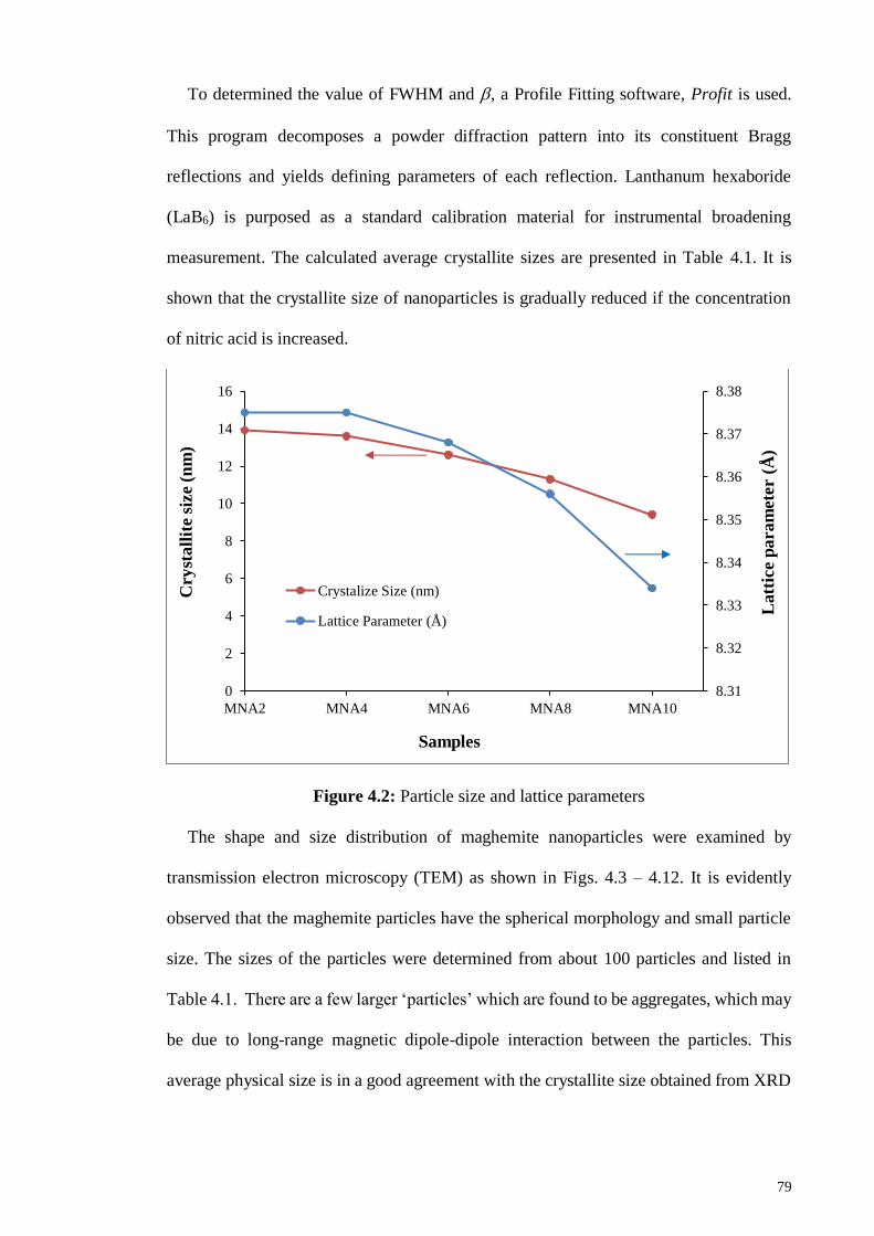
79
To determined the value of FWHM and , a Profile Fitting software, Profit is used.
This program decomposes a powder diffraction pattern into its constituent Bragg
reflections and yields defining parameters of each reflection. Lanthanum hexaboride
(LaB6) is purposed as a standard calibration material for instrumental broadening
measurement. The calculated average crystallite sizes are presented in Table 4.1. It is
shown that the crystallite size of nanoparticles is gradually reduced if the concentration
of nitric acid is increased.
Figure 4.2: Particle size and lattice parameters
The shape and size distribution of maghemite nanoparticles were examined by
transmission electron microscopy (TEM) as shown in Figs. 4.3 – 4.12. It is evidently
observed that the maghemite particles have the spherical morphology and small particle
size. The sizes of the particles were determined from about 100 particles and listed in
Table 4.1. There are a few larger ‘particles’ which are found to be aggregates, which may
be due to long-range magnetic dipole-dipole interaction between the particles. This
average physical size is in a good agreement with the crystallite size obtained from XRD
8.31
8.32
8.33
8.34
8.35
8.36
8.37
8.38
0
2
4
6
8
10
12
14
16
MNA2 MNA4 MNA6 MNA8 MNA10
Latt
ice p
aram
ete
r (Å
)
Cry
sta
llit
e s
ize (
nm
)
Samples
Crystalize Size (nm)
Lattice Parameter (Å)

80
measurement indicating that the particles are mostly monocrystals. It can also be seen that
the particles show normal size distribution.
Figure 4.3: TEM images of maghemite nanoparticles for samples MNA2
Figure 4.4: Particle distribution for maghemite nanoparticles for samples MNA2
50 nm nnnn
m
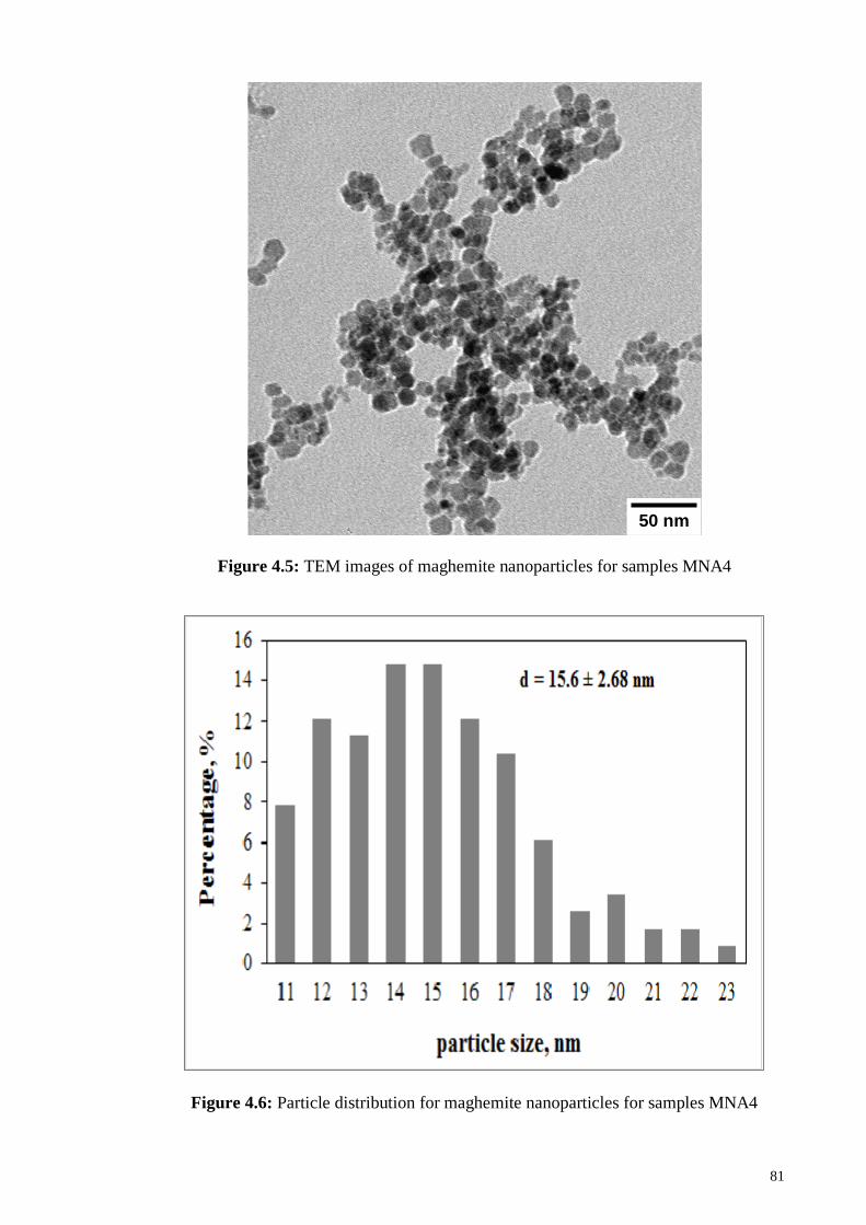
81
Figure 4.5: TEM images of maghemite nanoparticles for samples MNA4
Figure 4.6: Particle distribution for maghemite nanoparticles for samples MNA4
50 nm
nm

82
Figure 4.7: TEM images of maghemite nanoparticles for samples MNA6
Figure 4.8: Particle distribution for maghemite nanoparticles for samples MNA6
50 nm

83
Figure 4.9: TEM images of maghemite nanoparticles for samples MNA8
Figure 4.10: Particle distribution for maghemite nanoparticles for samples MNA8
50 nm

84
Figure 4.11: TEM images of maghemite nanoparticles for samples MNA10
Figure 4.12: Particle distribution for maghemite nanoparticles for samples MNA10
50 nm

85
The magnetization curve of the maghemite nanoparticle is shown in Fig. 4.13. It is
clear that the curves do not exhibit hysteresis and passes through the origin, which
indicates that the samples are superparamagnetic. The saturation magnetization values of
maghemite nanoparticle at room temperature for samples MNA2, MNA4, MNA6,
MNA8, and MNA10 are 42.4, 38.6, 36.6, 34.2, and 32.1 emu/g, respectively and the data
are presented in Table 4.1. These values are smaller than that of bulk maghemite (74
emu/g). This condition is related to the crystallite size of maghemite particles that are in
nanosize range. This phenomenon is usually observed in nanoparticle interacting systems.
Such a decreasing of magnetization can be ascribed to surface effects arising from broken
symmetry and reduced coordination of atoms lying at the surface of maghemite
nanoparticles. It is also caused by a high degree of interparticle interactions (Kluchova et
al., 2009).
Figure 4.13: Magnetization curve of maghemite nanoparticles for all samples
-50
-40
-30
-20
-10
0
10
20
30
40
50
-10 -5 0 5 10
Magn
eti
zati
on
(em
u/g
)
Applied field (kOe)
MNA2
MNA4
MNA6
MNA8
MNA10

86
TGA curves of the maghemite nanoparticle at different nitric acid concentration are
shown in Fig. 4.14. It can be seen that the curves reveal similar weight loss behavior and
display two weight loss steps. The first weight loss is associated with the evaporation of
absorbed water and crystalline water from the sample. The final weight loss might be
attributed to the volatilization of the remainder bonding water in the sample which
evaporated at the critical temperature of 374 oC. No further significant weight loss or gain
is found in the temperature range of 400 to 1000 oC, indicating crystalline of maghemite
has been formed completely. The temperature stability (Ts) for all samples when
maghemite entirely formed is presented in Table 4.1. It was displayed that the temperature
stability reduces with increasing concentration of nitric acid. This phenomenon indicates
that sample with the most concentrated nitric acid is stabilized earlier than other samples.
Figure 4.14: TGA thermogram of maghemite nanoparticles for all samples
26
28
30
32
34
36
38
40
0 100 200 300 400 500 600 700 800 900 1000
Weig
ht
(mg)
Temperature (oC)
MNA2
MNA4
MNA6
MNA8
MNA10

87
The particle size distributions of maghemite nanofluids obtained from dynamic light
scattering (DLS) measurement are shown in Fig. 4.15. The averaged particle size of
maghemite nanoparticles for all samples are listed in Table 4.1, indicates that the increase
of nitric acid concentration maghemite nanoparticles with decreasing diameter. High
concentration of nitric acid will suppress double layer of ions around the particles,
enhancing the diffusion speed and resulting smaller hydrodynamic diameter. It is also
displayed that the particle sizes obtained are larger than the TEM results due to the
hydrodynamic diameter of particles and its surrounding solvent layers.
Figure 4.15: DLS measurement of maghemite nanoparticles for all samples
The stability of the suspension is related to its electrokinetics properties. Therefore,
the study of electrophoretic behavior through measurement of zeta potential becomes
necessary for understanding the stability of suspension (Singh et al., 2005). It is
recognized that nanoparticles suspension become stable with a zeta potential value higher
than ± 30 mV. The zeta potential of maghemite nanofluids is shown in Fig. 4.16 and their
0
5
10
15
20
25
30
35
40
45
50
0 50 100 150 200 250 300 350 400 450 500
Inte
nsi
ty (
%)
Diameter (nm)
MNA2
MNA4
MNA6
MNA8
MNA10
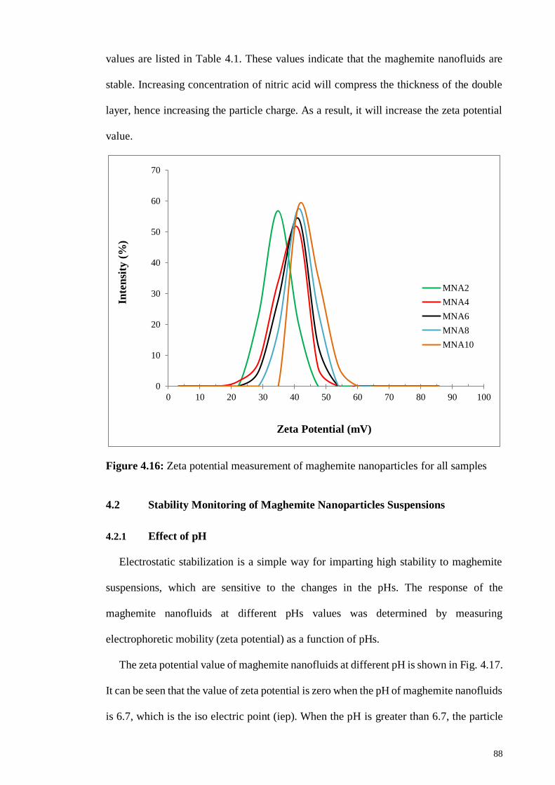
88
values are listed in Table 4.1. These values indicate that the maghemite nanofluids are
stable. Increasing concentration of nitric acid will compress the thickness of the double
layer, hence increasing the particle charge. As a result, it will increase the zeta potential
value.
Figure 4.16: Zeta potential measurement of maghemite nanoparticles for all samples
4.2 Stability Monitoring of Maghemite Nanoparticles Suspensions
4.2.1 Effect of pH
Electrostatic stabilization is a simple way for imparting high stability to maghemite
suspensions, which are sensitive to the changes in the pHs. The response of the
maghemite nanofluids at different pHs values was determined by measuring
electrophoretic mobility (zeta potential) as a function of pHs.
The zeta potential value of maghemite nanofluids at different pH is shown in Fig. 4.17.
It can be seen that the value of zeta potential is zero when the pH of maghemite nanofluids
is 6.7, which is the iso electric point (iep). When the pH is greater than 6.7, the particle
0
10
20
30
40
50
60
70
0 10 20 30 40 50 60 70 80 90 100
Inte
nsi
ty (
%)
Zeta Potential (mV)
MNA2
MNA4
MNA6
MNA8
MNA10

89
surface begins to have a negative charge. On the other hand, if suspension’s pH is lower
than 6.7, the particle surface has a positive charge. The value of zeta potential is higher
when the pH of the suspension is far from the IEP.
It is shown that the highest value of zeta potential is 44.6 mV at pH 3.60 at the acidic
condition and -46.2 mV at pH 10.50 at the alkaline condition. It is related to the smaller
particle size at a higher zeta potential value. The particle size is 45.3 nm at zeta potential
of 44.6 mV while, at the iso electric point, the particle size is 6560 nm. This phenomenon
is due to the particles surface charge is lower at the IEP. Hence, the particles are become
greater because of the agglomeration and aggregation of the particles in fluids. On the
other hand, as the pH of the fluids far from IEP, the particles surface charge become
higher. Hence, there is a resistance of the particles to agglomerate that give the particles
in suspension is become smaller.
The suspension has electrostatic stability due to the strong repulsive force between
charged particles. At the lower pH (acidic condition) and higher pH (alkaline condition),
the particles create high surface charge that result in higher zeta potential values. This
condition provides enough electrostatic repulsion force between particles to prevent
attraction and collision caused by Brownian motion.

90
Figure 4.17: Particle size and zeta potential measurement
of maghemite nanofluids at different pH
4.2.2 Effect of Time
Dynamic light scattering (DLS) and zeta potential characterizations were performed
to investigate the stability of maghemite nanofluids. The characterization was conducted
on the as-synthesized suspension and for the same suspension after two, four, and eight
months of storage at ambient conditioned. The results are shown in Figs. 4.18 and 4.19.
The averaged particle size of the maghemite nanoparticles is 45.3 nm. The average
sizes for sample after two, four, and eight months of storage are 47.1, 50.5, and 52.1 nm,
respectively. Table 4.5 summarize the results. The rise in the average particle size after
prolonged of storage indicates that a small degree of agglomeration was occurred. It can
be stated that although the nanofluids are very stable, the particle still grows due to the
growth of the particle nucleaus. Hence, the particles rise in a small degree with elapsed
time. However, there is no significant agglomeration and sedimentation was visually
observed on the maghemite nanofluids even after eight months of storage.
-60
-50
-40
-30
-20
-10
0
10
20
30
40
50
60
0
500
1000
1500
2000
2500
3000
3500
4000
4500
5000
5500
6000
6500
7000
7500
0 1 2 3 4 5 6 7 8 9 10 11 12 13
Zeta
pote
nti
al
(mV
)
Parti
cle
siz
e (
nm
)
pH
Particle size
Zeta Potential
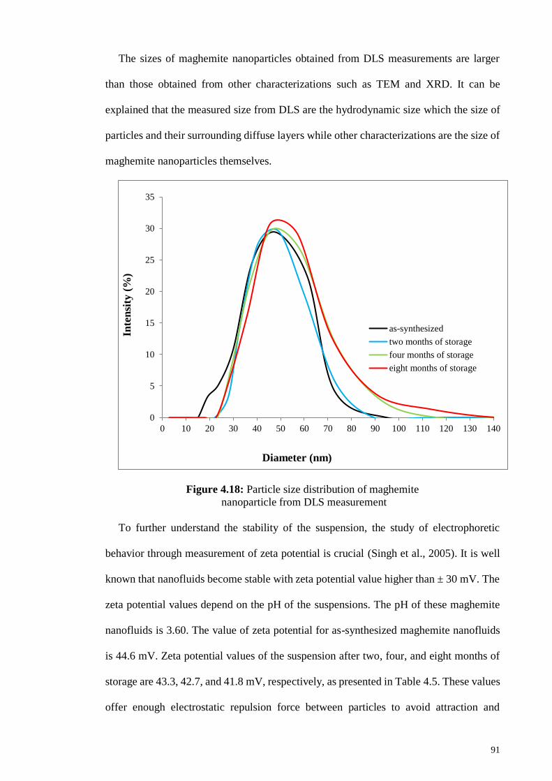
91
The sizes of maghemite nanoparticles obtained from DLS measurements are larger
than those obtained from other characterizations such as TEM and XRD. It can be
explained that the measured size from DLS are the hydrodynamic size which the size of
particles and their surrounding diffuse layers while other characterizations are the size of
maghemite nanoparticles themselves.
Figure 4.18: Particle size distribution of maghemite
nanoparticle from DLS measurement
To further understand the stability of the suspension, the study of electrophoretic
behavior through measurement of zeta potential is crucial (Singh et al., 2005). It is well
known that nanofluids become stable with zeta potential value higher than ± 30 mV. The
zeta potential values depend on the pH of the suspensions. The pH of these maghemite
nanofluids is 3.60. The value of zeta potential for as-synthesized maghemite nanofluids
is 44.6 mV. Zeta potential values of the suspension after two, four, and eight months of
storage are 43.3, 42.7, and 41.8 mV, respectively, as presented in Table 4.5. These values
offer enough electrostatic repulsion force between particles to avoid attraction and
0
5
10
15
20
25
30
35
0 10 20 30 40 50 60 70 80 90 100 110 120 130 140
Inte
nsi
ty (
%)
Diameter (nm)
as-synthesized
two months of storage
four months of storage
eight months of storage

92
collision caused by Brownian motion. This situation causes the maghemite nanofluids to
remain stable even after eight months of storage.
Figure 4.19: Zeta potential curves of maghemite nanofluids
Table 4.5 : Particle size and zeta potential measurement at various time of storage
Samples Particle size (nm) Zeta Potential (mV)
As-synthesized 45.3 44.6
Two months 47.1 43.3
Four months 50.5 42.7
Eight months 52.1 41.8
0
10
20
30
40
50
60
70
0 10 20 30 40 50 60 70 80 90 100
Inte
nsi
ty (
%)
Zeta Potential (mV)
as-synthesized
two months of storage
four months of storage
eight months of storage

93
4.3 Thermophysical Properties of Maghemite Nanofluids
4.3.1 Effect of Particle Volume Fraction
4.3.1.1 Thermal Conductivity of maghemite nanofluids
The thermal conductivity of maghemite nanofluids at a various particle volume
fraction and their standard deviations are presented in Table 4.6, while the graphs of
thermal conductivity measurement and their regression line are shown in Fig. 4.20. The
regression line and their degree of determination are tabulated in Table 4.7.
Overall, the thermal conductivities of the maghemite nanofluids increase linearly with
particles volume fraction and significantly higher than that of the corresponding base
fluids. This phenomenon is due to the particles have larger thermal conductivity than base
liquid. The suspended of a particle into base liquids improve the thermal conductivity of
suspensions that effect the maghemite nanofluids having larger thermal conductivity than
pure base liquid. The mixture of the nanofluids contains of three components, namely
nanoparticle, interfacial layer and liquids (Fu & Gao, 2012; Murshed et al., 2008; Tillman
& Hill, 2007). When the nanoparticles are suspended in the base fluids, interaction was
occurred between nanoparticles, interfacial layer and base fluids. These interactions are
caused by random movement of the particles in the base fluids due to collisions with the
molecules of base fluids (Godson et al., 2010). Besides that, there is also consideration
towards the effect of the interfacial layer between fluids and particles as the increase of
layer thickness increases the thermal conductivity of nanofluids. (Mintsa et al., 2009).
It can also be observed that the thermal conductivity of maghemite nanofluids is
linearly increased with increasing particle volume fraction at a certain temperature. This
condition is due to higher particle volume fraction, there are more particles suspended in
the base liquid. At the same time, the conductivity was increased as the temperature
increases due to the increase of maghemite nanoparticles Brownian motion. Hence,
maghemite nanofluids have higher thermal conductivity.

94
Table 4.6: Thermal conductivity of maghemite nanofluids
at different particle volume fractions
Particle
volume fraction
(%)
Thermal conductivity (W/mK)
T : 10 oC T : 15 oC T : 20 oC
0.0 0.578 ± 0.0007 0.586 ± 0.0008 0.595 ± 0.0010
0.1 0.580 ± 0.0015 0.589 ± 0.0015 0.599 ± 0.0013
0.2 0.583 ± 0.0011 0.592 ± 0.0013 0.603 ± 0.0011
0.3 0.588 ± 0.0017 0.597 ± 0.0016 0.606 ± 0.0011
0.4 0.593 ± 0.0015 0.602 ± 0.0019 0.611 ± 0.0015
0.5 0.596 ± 0.0019 0.605 ± 0.0011 0.616 ± 0.0013
0.6 0.599 ± 0.0015 0.612 ± 0.0016 0.621 ± 0.0018
Particle
volume fraction
(%)
Thermal conductivity (W/mK)
T : 25 oC T : 30 oC T : 35 oC
0.0 0.602 ± 0.0013 0.614 ± 0.0016 0.621 ± 0.0008
0.1 0.607 ± 0.0016 0.620 ± 0.0017 0.634 ± 0.0022
0.2 0.617 ± 0.0010 0.634 ± 0.0013 0.651± 0.0017
0.3 0.622 ± 0.0019 0.645 ± 0.0018 0.672 ± 0.0016
0.4 0.627 ± 0.0015 0.657 ± 0.0013 0.685 ± 0.0019
0.5 0.631 ± 0.0018 0.668 ± 0.0019 0.704 ± 0.0018
0.6 0.642 ± 0.0011 0.689 ± 0.0016 0.738 ± 0.0015
Figure 4.20: Thermal conductivity of maghemite nanofluids
as a function of particle volume fraction at different temperatures.
0.56
0.58
0.60
0.62
0.64
0.66
0.68
0.70
0.72
0.74
0.76
0.0 0.1 0.2 0.3 0.4 0.5 0.6
Th
erm
al
Con
du
cti
vit
y (
W/m
K)
Particle volume fraction (%)
T : 10 °CT : 15 °CT : 20 °CT : 25 °CT : 30 °CT : 35 °Cregression line
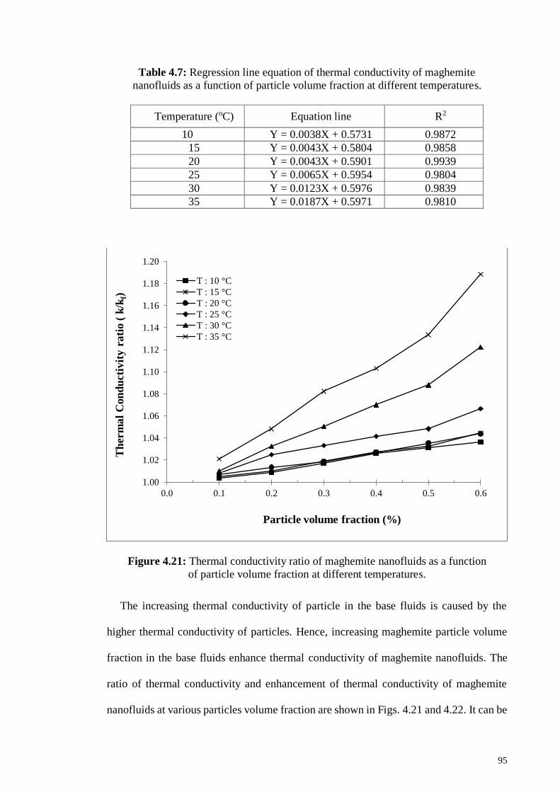
95
Table 4.7: Regression line equation of thermal conductivity of maghemite
nanofluids as a function of particle volume fraction at different temperatures.
Temperature (oC) Equation line R2
10 Y = 0.0038X + 0.5731 0.9872
15 Y = 0.0043X + 0.5804 0.9858
20 Y = 0.0043X + 0.5901 0.9939
25 Y = 0.0065X + 0.5954 0.9804
30 Y = 0.0123X + 0.5976 0.9839
35 Y = 0.0187X + 0.5971 0.9810
Figure 4.21: Thermal conductivity ratio of maghemite nanofluids as a function
of particle volume fraction at different temperatures.
The increasing thermal conductivity of particle in the base fluids is caused by the
higher thermal conductivity of particles. Hence, increasing maghemite particle volume
fraction in the base fluids enhance thermal conductivity of maghemite nanofluids. The
ratio of thermal conductivity and enhancement of thermal conductivity of maghemite
nanofluids at various particles volume fraction are shown in Figs. 4.21 and 4.22. It can be
1.00
1.02
1.04
1.06
1.08
1.10
1.12
1.14
1.16
1.18
1.20
0.0 0.1 0.2 0.3 0.4 0.5 0.6
Th
erm
al
Con
du
cti
vit
y r
ati
o (
k/k
f)
Particle volume fraction (%)
T : 10 °C
T : 15 °C
T : 20 °C
T : 25 °C
T : 30 °C
T : 35 °C

96
seen that the increased thermal conductivity is higher at a higher particle volume fraction
of maghemite nanoparticles. This phenomenon is due to more particles were involved in
base fluids that have higher thermal conductivity compared to base fluids. This result is
in conformity with others (Abareshi et al., 2010; Gavili et al., 2012; Pastoriza-Gallego et
al., 2011; Phuoc et al., 2011). Hence, at a higher particle volume fraction, the thermal
conductivity of maghemite nanofluids is larger than that of lower particles volume
fractions. The highest enhancement of thermal conductivity of maghemite nanoparticles
suspensions is 18.84 % achieved at a particle volume fraction of 0.6 % at a temperature
of 35 oC.
Figure 4.22: Enhancement of thermal conductivity of maghemite nanofluids
as a function of particle volume fraction at different temperatures.
4.3.1.2 Kinematic viscosity of maghemite nanofluids
Kinematic viscosity of maghemite nanofluids at a various particle volume fraction and
their standard deviation of measurements are tabulated in Table 4.8. The graphs of the
trend of the kinematic viscosity of maghemite nanofluids are shown in Fig. 4.23. The
0
2
4
6
8
10
12
14
16
18
20
0.0 0.1 0.2 0.3 0.4 0.5 0.6
Th
erm
al
con
du
cti
vit
y i
ncre
ase
d (
%)
Particle volume fraction (%)
T : 10 °C
T : 15 °C
T : 20 °C
T : 25 °C
T : 30 °C
T : 35 °C

97
regression line equations and their coefficient of determinations are tabulated in Table
4.9. The kinematic viscosity ratio and percentage of kinematic viscosity enhancement are
given in Figs. 4.24 and 4.25. The viscosity depends on the particles volume fraction of
maghemite nanoparticle. Increasing particle concentration will enhance the viscosity of
maghemite nanofluids. Once the nanoparticles are dispersed in the solution, there is
possibility of enhancement in resistance between the two layers of liquid.
As a nanofluid is a mixture of nanoparticles and base fluids, there is an interaction
between particles and its surrounding. The flow of nanofluids created a friction between
nanofluids and its surrounding that resist the flow of nanofluids. The more concentrated
of nanoparticles in the fluids will enhance the resistance of nanofluids flow, and this will
enhance the viscosity of nanofluids. The highest enhancement of the kinematic viscosity
of maghemite nanofluids is 13.66 % for a particle volume fraction of 0.6 % and
temperature of 35 oC.
Table 4.8: Kinematic viscosity of maghemite nanofluids
at different particle volume fractions
Particle
volume fraction
(%)
Kinematic viscosity (cst)
T : 10 oC T : 15 oC T : 20 oC
0.0 1.307 ± 0.0019 1.144 ± 0.0015 0.997 ± 0.0023
0.1 1.316 ± 0.0016 1.148 ± 0.0023 1.010 ± 0.0023
0.2 1.319 ± 0.0018 1.151 ± 0.0028 1.018 ± 0.0013
0.3 1.323 ± 0.0017 1.155 ± 0.0020 1.032 ± 0.0016
0.4 1.328 ± 0.0019 1.160 ± 0.0020 1.036 ± 0.0017
0.5 1.332 ± 0.0019 1.166 ± 0.0018 1.041 ± 0.0016
0.6 1.337 ± 0.0012 1.172 ± 0.0016 1.053 ± 0.0019
Particle
volume fraction
(%)
Kinematic viscosity (cst)
T : 25 oC T : 30 oC T : 35 oC
0.0 0.889 ± 0.0019 0.799 ± 0.0011 0.732 ± 0.0012
0.1 0.901 ± 0.0026 0.812 ± 0.0017 0.748 ± 0.0018
0.2 0.922 ± 0.0018 0.835 ± 0.0015 0.767 ± 0.0018
0.3 0.945 ± 0.0020 0.856 ± 0.0020 0.789 ± 0.0017
0.4 0.957 ± 0.0012 0.868 ± 0.0014 0.805 ± 0.0019
0.5 0.968 ± 0.0022 0.881 ± 0.0017 0.816 ± 0.0009
0.6 0.976 ± 0.0014 0.893 ± 0.0020 0.832 ± 0.0017

98
Figure 4.23: Viscosity of maghemite nanofluids as a function of
particle volume fraction at different temperatures.
Table 4.9: Regression line equation of kinematic viscosity of maghemite
nanofluids as a function of particle volume fraction.
Temperature (oC) Equation line R2
10 Y = 0.0047X + 1.3044 0.9840
15 Y = 0.0046X + 1.1381 0.9844
20 Y = 0.0089X + 0.9913 0.9774
25 Y = 0.0154X + 0.8754 0.9753
30 Y = 0.0162X + 0.7844 0.9857
35 Y = 0.0169X + 0.7164 0.9927
0.7
0.8
0.9
1.0
1.1
1.2
1.3
1.4
1.5
1.6
0.0 0.1 0.2 0.3 0.4 0.5 0.6
Kin
em
ati
c v
iscosi
ty (
cst
)
Particle volume fraction (%)
T:10 °C T:15 °C
T:20 °C T:25 °C
T:30 °C T:35 °C
regression line
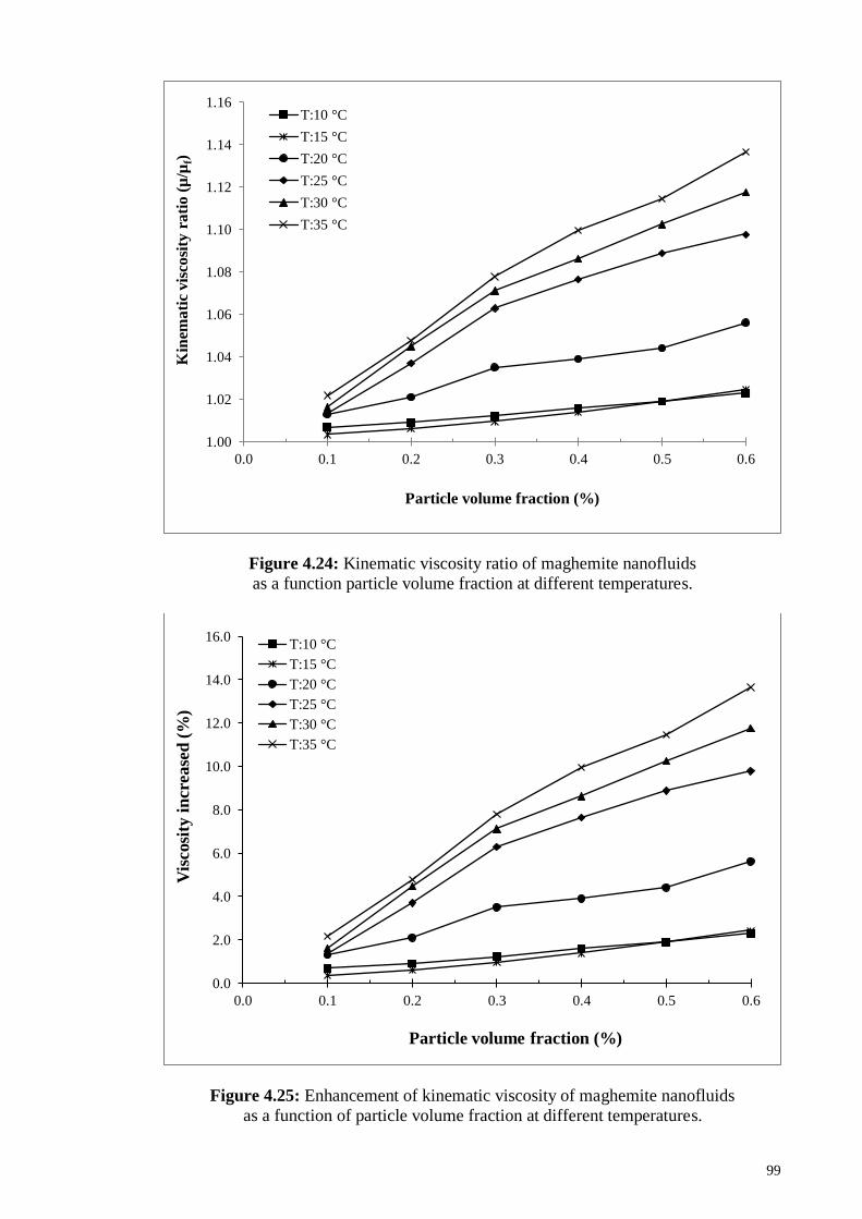
99
Figure 4.24: Kinematic viscosity ratio of maghemite nanofluids
as a function particle volume fraction at different temperatures.
Figure 4.25: Enhancement of kinematic viscosity of maghemite nanofluids
as a function of particle volume fraction at different temperatures.
1.00
1.02
1.04
1.06
1.08
1.10
1.12
1.14
1.16
0.0 0.1 0.2 0.3 0.4 0.5 0.6
Kin
ema
tic
vis
cosi
ty r
ati
o (
µ/µ
f)
Particle volume fraction (%)
T:10 °C
T:15 °C
T:20 °C
T:25 °C
T:30 °C
T:35 °C
0.0
2.0
4.0
6.0
8.0
10.0
12.0
14.0
16.0
0.0 0.1 0.2 0.3 0.4 0.5 0.6
Vis
cosi
ty i
ncre
ase
d (
%)
Particle volume fraction (%)
T:10 °C
T:15 °C
T:20 °C
T:25 °C
T:30 °C
T:35 °C

100
4.3.1.3 Electrical Conductivity
Electrical conductivity of maghemite nanofluids and their standard deviation of
measurements are tabulated in Table 4.10. The electrical conductivity of maghemite
nanofluids are shown in Fig. 4.26. The regression line and their degree of conformity are
presented in Table 4.11. The percentage of enhancement of maghemite nanofluids at
various particle volume fractions is given in Fig. 4.27.
It can be seen from Fig. 4.26 that the electrical conductivity of maghemite nanofluids
increases almost linearly with increase in volume fraction of the maghemite
nanoparticles. The experimental data also indicates that for a given volume fraction, the
electrical conductivity of the suspension increases with the temperature. The highest
value of electrical conductivity was 7.348 mS/cm recorded for a volume fraction of 0.6
% at a temperature of 35 oC. The corresponding values at room temperature (25 oC) was
6.617 mS/cm and the lowest temperature (10 oC) was 4.046 mS/cm. These conductivity
values are much higher (with ordering of 3) when compared with the electrical
conductivity values of magnetite nanoparticles obtained by Bagheli (Bagheli et al., 2015).
This phenomenon is due to the electrical conductivity of colloidal nano suspensions in
a fluid exhibits a complicated dependence on the electrical double layers. It also depends
on characteristics, volume fraction, ionic concentrations and other physicochemical
properties (Modesto-Lopez & Biswas, 2010).
When maghemite nanoparticles are suspended in a polar liquid like water, electrical
charges are developing on the surfaces. Ions opposite to that relating to the particle surface
are attracted, causing the creation of a charged diffuse layer all around the particle. The
surface charge of the particles, as well as ion-cloud that constitutes the EDL actively plays
a part in the enhancement of conduction mechanisms through the suspension.
Furthermore, the existence of uniformly dispersed nanoparticles is considered by reduced
equivalent particulate masses, leading to increased electrophoretic mobility, which

101
consequently enhance the electrical conductivity of the maghemite nanofluids. With
increasing of particle volume fraction in the solution, more conducting pathway in the
solutions are formed, that in turn enhances the overall electrical conductivity of the
solution.
The enhancement of electrical conductivity of maghemite nanofluids is presented in
Fig. 4.27. For those purpose, the rate of enhancement of the electrical conductivity desired
as the different between the electrical conductivity of the nanoparticle suspension and the
electrical conductivity of the base fluids divided by the electrical conductivity of the base
fluids. As shown in Fig. 4.27, the enhancement increases with respect to increase in
nanoparticle volume fraction, which indicate a dependence on volume fraction. This
variation also depends on the temperature, where the higher the temperature, the greater
is the enhancement. A 100.3 % increase in the electrical conductivity was observed for
0.2 % volume concentration of maghemite nanoparticles in water at temperature 35 oC.
With rise in volume fraction (0.6 %), a 567 % increase in the electrical conductivity was
measured for the same temperature of 35 oC.
Table 4.10 : Electrical conductivity of maghemite nanofluids as
a function of particle volume fraction at different temperatures.
Particle
volume fraction
(%)
Electrical conductivity (mS/cm)
T : 10 oC T : 15 oC T : 20 oC
0.1 0.868± 0.0011 0.947± 0.0010 0.990 ± 0.0016
0.2 1.461± 0.0013 1.645± 0.0018 1.814 ± 0.0016
0.3 2.165± 0.0016 2.561± 0.0013 2.819 ± 0.0013
0.4 2.754± 0.0015 3.318± 0.0011 3.688 ± 0.0014
0.5 3.378± 0.0003 4.204± 0.0019 4.643 ± 0.0010
0.6 4.046± 0.0011 5.194± 0.0016 5.673 ± 0.0013
Particle
volume fraction
(%)
Electrical conductivity (mS/cm)
T : 25 oC T : 30 oC T : 35 oC
0.1 1.010 ± 0.0013 1.051 ± 0.0016 1.102 ± 0.0011
0.2 1.986 ± 0.0012 2.168 ± 0.0011 2.376 ± 0.0007
0.3 3.109 ± 0.0016 3.375 ± 0.0016 3.644 ± 0.0011
0.4 4.017 ± 0.0019 4.367 ± 0.0008 4.745 ± 0.0007
0.5 4.991 ± 0.0016 5.456 ± 0.0013 5.998 ± 0.0009
0.6 6.617 ± 0.0020 6.681 ± 0.0010 7.348 ± 0.0018

102
Figure 4.26: Electrical conductivity of maghemite nanofluids as
a function of particle volume fraction at different temperatures.
Table 4.11: Regression line equation of electrical conductivity of
Maghemite nanofluids at various particle volume fractions.
Temperature (oC) Equation line R2
10 Y = 6.3514X + 0.2223 0.9996
15 Y = 8.4769X + 0.0113 0.9976
20 Y = 9.3631X – 0.0059 0.9991
25 Y = 10.202X – 0.0241 0.9989
30 Y = 11.145X – 0.0509 0.9993
35 Y = 12.342X – 0.1175 0.9994
0.0
1.0
2.0
3.0
4.0
5.0
6.0
7.0
8.0
0.0 0.1 0.2 0.3 0.4 0.5 0.6
Ele
ctr
ical con
du
cti
vit
y (
mS
/cm
)
Volume fraction (%)
T : 10 °C
T : 15 °C
T : 20 °C
T : 25 °C
T : 30 °C
T : 35 °C
regression line

103
Figure 4.27: Enhancement of electrical conductivity of maghemite nanofluids
as a function of particle volume fraction at different temperatures.
4.3.2 Effect of Temperature
4.3.2.1 Thermal Conductivity
The thermal conductivities of maghemite nanofluids and their standard deviation of
measurements are tabulated in Table 4.12. The effect of temperature on thermal
conductivity of maghemite nanofluids is shown in Fig. 4.28. The regression line and
degree of conformity of measurement are tabulated in Table 4.13. The thermal
conductivity ratio and percentage of enhancement of maghemite nanofluids at various
temperatures are shown in Figs. 4.29 and 4.30.
The thermal conductivities are nonlinearly increases with the increase of temperature.
When the temperature rises, the intensity of Brownian motion augments greatly, which
leads to a corresponding enhancement of thermal conductivity. The thermal conductivity
of high volume fraction of maghemite become larger than that with lower volume fraction
0
100
200
300
400
500
600
0.0 0.1 0.2 0.3 0.4 0.5 0.6
Ele
ctr
ical C
on
du
cti
vit
y i
ncre
ase
d (
%)
Particle volume fraction (%)
T : 10 °C
T : 15 °C
T : 20 °C
T : 25 °C
T : 30 °C
T : 35 °C
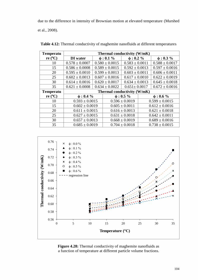
104
due to the difference in intensity of Brownian motion at elevated temperature (Murshed
et al., 2008).
Table 4.12: Thermal conductivity of maghemite nanofluids at different temperatures
Temperatu
re (oC)
Thermal conductivity (W/mK)
DI water ϕ : 0.1 % ϕ : 0.2 % ϕ : 0.3 %
10 0.578 ± 0.0007 0.580 ± 0.0015 0.583 ± 0.0011 0.588 ± 0.0017
15 0.586 ± 0.0008 0.589 ± 0.0015 0.592 ± 0.0013 0.597 ± 0.0016
20 0.595 ± 0.0010 0.599 ± 0.0013 0.603 ± 0.0011 0.606 ± 0.0011
25 0.602 ± 0.0013 0.607 ± 0.0016 0.617 ± 0.0010 0.622 ± 0.0019
30 0.614 ± 0.0016 0.620 ± 0.0017 0.634 ± 0.0013 0.645 ± 0.0018
35 0.621 ± 0.0008 0.634 ± 0.0022 0.651± 0.0017 0.672 ± 0.0016
Temperatu
re (oC)
Thermal conductivity (W/mK)
ϕ : 0.4 % ϕ : 0.5 % ϕ : 0.6 %
10 0.593 ± 0.0015 0.596 ± 0.0019 0.599 ± 0.0015
15 0.602 ± 0.0019 0.605 ± 0.0011 0.612 ± 0.0016
20 0.611 ± 0.0015 0.616 ± 0.0013 0.621 ± 0.0018
25 0.627 ± 0.0015 0.631 ± 0.0018 0.642 ± 0.0011
30 0.657 ± 0.0013 0.668 ± 0.0019 0.689 ± 0.0016
35 0.685 ± 0.0019 0.704 ± 0.0018 0.738 ± 0.0015
Figure 4.28: Thermal conductivity of maghemite nanofluids as
a function of temperature at different particle volume fractions.
0.56
0.58
0.60
0.62
0.64
0.66
0.68
0.70
0.72
0.74
0.76
0 5 10 15 20 25 30 35
Th
erm
al
con
du
cti
vit
y (
W/m
K)
Temperature (°C)
ϕ : 0.0 %
ϕ : 0.1 %
ϕ : 0.2 %
ϕ : 0.3 %
ϕ : 0.4 %
ϕ : 0.5 %
ϕ : 0.6 %
regression line

105
Table 4.13: Regression line equation of thermal conductivity of
maghemite nanofluids as a function of temperature.
Particle volume
fraction (%)
Equation line R2
0.0 Y = 5E-06X2+0.0015X+0.5622 0.9962
0.1 Y = 3E-05X2+0.0009X+0.5686 0.9979
0.2 Y = 5E-05X2+0.0007X+0.5714 0.9962
0.3 Y = 1E-04X2−0.0014X+0.5923 0.9988
0.4 Y = 1E-04X2−0.0021X+0.6022 0.9965
0.5 Y = 2E-04X2−0.0034X+0.6150 0.9949
0.6 Y = 2E-04X2 −0.0051X+0.6300 0.9944
Figure 4.29: Thermal conductivity ratio of maghemite nanofluids as
a function of temperature at different particle volume fractions.
1.00
1.02
1.04
1.06
1.08
1.10
1.12
1.14
1.16
1.18
1.20
0 5 10 15 20 25 30 35
Th
erm
al
con
du
cti
vit
y r
ati
o (
k/k
f)
Temperature (°C)
ϕ : 0.1 %
ϕ : 0.2 %
ϕ : 0.3 %
ϕ : 0.4 %
ϕ : 0.5 %
ϕ : 0.6 %

106
Figure 4.30: Enhancement of thermal conductivity of maghemite as
a function of temperature at different particle volume fractions.
From Fig 4.30, it can be seen that high degree of enhancement of thermal conductivity
of maghemite nanofluids at higher temperature. At lower temperature, the particles are
tightly bound within suspension, hence slower movement of the particles in the solution.
On the other hand, at higher temperature, there are more mobile particles movement
rapidly in the solution. Increasing temperature of suspensions will increase nonlinearly
the thermal conductivity of suspensions. Since temperature are significantly effects
thermal conductivity by randomly increasing of the molecular movement in the
suspension.
4.3.2.2 Kinematic Viscosity
Kinematic viscosity of maghemite nanofluids at different temperatures and their
standard deviation measurements are tabulated in Table 4.14. The graphs of kinematic
viscosity of maghemite nanofluids at different temperatures are presented in Fig. 4.31.
The regression line equations and their coefficient of determinations are tabulated in
0.00
2.00
4.00
6.00
8.00
10.00
12.00
14.00
16.00
18.00
20.00
0 5 10 15 20 25 30 35
Th
erm
al
con
du
cti
vit
y i
ncre
ase
d (
%)
Temperature (°C)
ϕ : 0.1 %
ϕ : 0.2 %
ϕ : 0.3 %
ϕ : 0.4 %
ϕ : 0.5 %
ϕ : 0.6 %
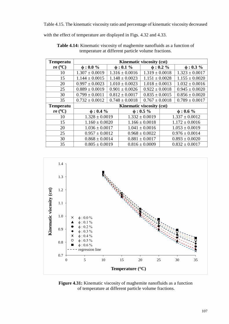
107
Table 4.15. The kinematic viscosity ratio and percentage of kinematic viscosity decreased
with the effect of temperature are displayed in Figs. 4.32 and 4.33.
Table 4.14: Kinematic viscosity of maghemite nanofluids as a function of
temperature at different particle volume fractions.
Temperatu
re (oC)
Kinematic viscosity (cst)
ϕ : 0.0 % ϕ : 0.1 % ϕ : 0.2 % ϕ : 0.3 %
10 1.307 ± 0.0019 1.316 ± 0.0016 1.319 ± 0.0018 1.323 ± 0.0017
15 1.144 ± 0.0015 1.148 ± 0.0023 1.151 ± 0.0028 1.155 ± 0.0020
20 0.997 ± 0.0023 1.010 ± 0.0023 1.018 ± 0.0013 1.032 ± 0.0016
25 0.889 ± 0.0019 0.901 ± 0.0026 0.922 ± 0.0018 0.945 ± 0.0020
30 0.799 ± 0.0011 0.812 ± 0.0017 0.835 ± 0.0015 0.856 ± 0.0020
35 0.732 ± 0.0012 0.748 ± 0.0018 0.767 ± 0.0018 0.789 ± 0.0017
Temperatu
re (oC)
Kinematic viscosity (cst)
ϕ : 0.4 % ϕ : 0.5 % ϕ : 0.6 %
10 1.328 ± 0.0019 1.332 ± 0.0019 1.337 ± 0.0012
15 1.160 ± 0.0020 1.166 ± 0.0018 1.172 ± 0.0016
20 1.036 ± 0.0017 1.041 ± 0.0016 1.053 ± 0.0019
25 0.957 ± 0.0012 0.968 ± 0.0022 0.976 ± 0.0014
30 0.868 ± 0.0014 0.881 ± 0.0017 0.893 ± 0.0020
35 0.805 ± 0.0019 0.816 ± 0.0009 0.832 ± 0.0017
Figure 4.31: Kinematic viscosity of maghemite nanofluids as a function
of temperature at different particle volume fractions.
0.7
0.8
0.9
1.0
1.1
1.2
1.3
1.4
0 5 10 15 20 25 30 35
Kin
em
ati
c v
iscosi
ty (
cst
)
Temperature (°C)
ϕ : 0.0 %
ϕ : 0.1 %
ϕ : 0.2 %
ϕ : 0.3 %
ϕ : 0.4 %
ϕ : 0.5 %
ϕ : 0.6 %
regression line

108
Table 4.15: Regression line equation of kinematic viscosity of maghemite nanofluids
as a function of temperature at different particle volume fractions.
Particle volume
fraction (%)
Equation line R2
0.0 Y = 0.0005X2 −0.0457X+1.7137 0.9999
0.1 Y = 0.0005X2 −0.0456X+1.7195 0.9999
0.2 Y = 0.0005X2 −0.0437X+1.7028 0.9992
0.3 Y = 0.0005X2 −0.0415X+1.6849 0.9981
0.4 Y = 0.0005X2 −0.0418X+1.6905 0.9974
0.5 Y = 0.0005X2 −0.0412X+1.6884 0.9965
0.6 Y = 0.0005X2 −0.0410X+1.6915 0.9972
It can be seen that the kinematic viscosity ratio of maghemite nanofluids are decreased
nonlinearly with the temperature. The liquid molecules are tightly bounded by attractive
inter-molecular forces (e.g. Van der Waal forces) at low temperature. These attractive
forces are responsible for the viscosity since the individual molecule is difficult to move
due to it tightly bounded to its neighbors. Therefore, the kinematic viscosity is larger at
low temperature.
The impact of increasing temperature weakened the inter-particle and inter-molecular
adhesion forces hence accelerate the movement of the particles in liquids (Nguyen et al.,
2007). The increase in temperature causes the increase of kinetic or thermal energy and
the molecules become more mobile. As a result, the viscosity is reduced. From Fig. 4.33,
it can also be seen that kinematic viscosity of maghemite nanofluids is linearly decreased
with increasing of temperature.

109
Figure 4.32: Kinematic viscosity ratio of maghemite nanofluids as
a function of temperature at different particle volume fractions.
Figure 4.33: Decreasing of kinematic viscosity of maghemite nanofluids as
a function of temperature at different particle volume fractions.
0.5
0.6
0.7
0.8
0.9
1.0
0 5 10 15 20 25 30 35
Kin
em
ati
c v
iscosi
ty r
ati
o (
cst
)
Temperature (oC)
ϕ : 0.0 %
ϕ : 0.1 %
ϕ : 0.2 %
ϕ : 0.3 %
ϕ : 0.4 %
ϕ : 0.5 %
ϕ : 0.6 %
-60.0
-50.0
-40.0
-30.0
-20.0
-10.0
0.0
0 5 10 15 20 25 30 35
Kin
em
ati
c v
iscosi
ty d
ecre
ase
d (
%)
Temperature (oC)
ϕ : 0.0 %
ϕ : 0.1 %
ϕ : 0.2 %
ϕ : 0.3 %
ϕ : 0.4 %
ϕ : 0.5 %
ϕ : 0.6 %

110
4.3.2.3 Electrical conductivity
Electrical conductivity of maghemite nanofluids at different temperature and their
standard deviation measurement are tabulated in Table 4.16. The graphs of electrical
conductivity of maghemite nanofluids at different temperatures are presented in Fig. 4.34.
The regression line equations and their coefficient of determinations are tabulated in
Table 4.17. The percentage of increasing of electrical conductivity of maghemite
nanofluids at various temperatures are presented in Fig. 4.35.
Table 4.16: Electrical conductivity of maghemite nanofluids as a function of
temperature at different particle volume fractions.
Temperature
(oC)
Electrical conductivity (mS/cm)
ϕ : 0.1 % ϕ : 0.2 % ϕ : 0.3 %
10 0.868± 0.0011 1.461± 0.0013 2.165± 0.0016
15 0.947± 0.0010 1.645± 0.0018 2.561± 0.0013
20 0.990 ± 0.0016 1.814 ± 0.0016 2.819 ± 0.0013
25 1.010 ± 0.0013 1.986 ± 0.0012 3.109 ± 0.0016
30 1.051 ± 0.0016 2.168 ± 0.0011 3.375 ± 0.0016
35 1.102 ± 0.0011 2.376 ± 0.0007 3.644 ± 0.0011
Temperature
(oC)
Electrical conductivity (mS/cm)
ϕ : 0.4 % ϕ : 0.5 % ϕ : 0.6 %
10 2.754± 0.0015 3.378± 0.0013 4.046± 0.0011
15 3.318± 0.0011 4.204± 0.0019 5.194± 0.0016
20 3.688 ± 0.0014 4.643 ± 0.0010 5.673 ± 0.0013
25 4.017 ± 0.0019 4.991 ± 0.0016 6.617 ± 0.0020
30 4.367 ± 0.0008 5.456 ± 0.0013 6.681 ± 0.0010
35 4.745 ± 0.0007 5.998 ± 0.0009 7.348 ± 0.0018
The experimental data indicate that for a given particle volume fraction, the electrical
conductivity of the maghemite nanofluids increases with the temperature. The increasing
of maghemite nanofluids is slower at lower temperature. As the temperature of the
maghemite nanofluids increase, it will decrease the viscosity and enhance the ions
mobility. Furthermore, it could also increase the number of ions in the solution due to
molecular dissociation. As a result, this will lead to an increase in its conductivity.

111
Figure 4.34: Electrical conductivity of maghemite nanofluids as
a function of temperature at different particle volume fractions.
Table 4.17: Regression line equation of electrical conductivity of maghemite
nanofluids as a function of temperature at different particle volume fractions.
Particle volume
fraction (%) Equation line R2
0.0
0.1 Y = 0.0086X + 0.8016 0.9688
0.2 Y = 0.0361X + 1.0963 0.9989
0.3 Y = 0.0579X + 1.6435 0.9952
0.4 Y = 0.0767X + 2.088 0.9914
0.5 Y = 0.0983X + 2.5664 0.9952
0.6 Y = 0.1227X + 3.0917 0.975
From Fig. 4.35, it is shown that the enhancement of electrical conductivity of
maghemite nanofluids increases almost linearly with temperature. This enhancement also
depends on the volume fraction as the higher the volume fraction, the greater its
enhancement. 52 % of enhancement in the electrical conductivity was recorded at room
temperature (25 oC) for 0.6 % of volume fraction. Meanwhile, 82 % of enhancement in
the electrical conductivity was recorded for the same volume fraction (0.6 %) at higher
0.0
1.0
2.0
3.0
4.0
5.0
6.0
7.0
8.0
0 5 10 15 20 25 30 35
Ele
ctr
ical con
du
cti
vit
y (
mS
/cm
)
Temperature (oC)
ϕ : 0.1%
ϕ : 0.2%
ϕ : 0.3%
ϕ : 0.4%
ϕ : 0.5%
ϕ : 0.6%
regression line

112
temperature of 35 oC. The electrical conductivity enhancement of maghemite nanofluids
due to temperature effect is lowered by first order compared to volume fraction effect.
These results are in good agreement with published data on other nanofluids (Dong et
al., 2013; Ganguly et al., 2009; Minea & Luciu, 2012; Sarojini et al., 2013; Shen et al.,
2012; Sikdar et al., 2011; Steven et al., 2011). However, the findings do not correlated
with the Maxwell (Maxwell, 1954) and Bruggeman models (Bruggeman, 1935) due to
these models do not take into account the temperature factor. This observation is also
supported by Sundar et al. (2014).
Figure 4.35: Enhancement of electrical conductivity of maghemite nanofluids
as a function of temperature at different particle volume fractions.
4.3.3 Effect of Magnetic Fields
The effect of magnetic fields on the properties of maghemite nanofluids was conducted
in a pair of Helmholtz coils, which arrange in perpendicular and parallel to the samples.
The measurements of the properties were performed with the effect of both arrangements
of the magnetic fields.
0.00
10.00
20.00
30.00
40.00
50.00
60.00
70.00
80.00
90.00
10 15 20 25 30 35
Ele
ctr
ical con
du
cti
vit
y i
ncre
ase
d (
%)
Temperature (oC)
ϕ : 0.1%
ϕ : 0.2%
ϕ : 0.3%
ϕ : 0.4%
ϕ : 0.5%
ϕ : 0.6%

113
The advantage of this system was one can control the particles aggregation with
different chain lengths. Due to the superparamagnetic nature of particles, the aggregation
phenomenon was perfectly reversible.
4.3.3.1 Thermal Conductivity
Data measurements and their standard deviation of thermal conductivity of maghemite
nanofluids under parallel magnetic fields arrangements is presented in Table 4.18. The
effect of magnetic fields strength on thermal conductivity of maghemite nanofluids for
parallel magnetic fields arrangements is shown in Fig. 4.36. The regression line equations
and their coefficient of determinations are tabulated in Table 4.19. Thermal conductivity
ratio of maghemite nanofluids and their percentage of enhancement are presented in Figs.
4.37 and 4.38.
Table 4.18: Thermal conductivity of maghemite nanofluids at
different parallel magnetic fields strength
Magnetic
fields strength
(Gauss)
Thermal conductivity (W/mK)
ϕ : 0.1 % ϕ : 0.2 % ϕ : 0.3 %
0 0.607 ± 0.0016 0.617 ± 0.0013 0.622± 0.0016
50 0.612 ± 0.0015 0.620 ± 0.0015 0.624 ± 0.0011
100 0.615 ± 0.0013 0.623 ± 0.0016 0.632 ± 0.0013
150 0.628 ± 0.0016 0.635 ± 0.0018 0.642 ± 0.0015
200 0.640 ± 0.0017 0.654 ± 0.0016 0.663 ± 0.0013
250 0.650 ± 0.0016 0.667 ± 0.0018 0.682 ± 0.0011
300 0.662 ± 0.0013 0.681 ± 0.0017 0.711 ± 0.0015
Magnetic
fields strength
(Gauss)
Thermal conductivity (W/mK)
ϕ : 0.4 % ϕ : 0.5 % ϕ : 0.6 %
0 0.627 ± 0.0012 0.632 ± 0.0016 0.643 ± 0.0011
50 0.631 ± 0.0013 0.635 ± 0.0016 0.647 ± 0.0012
100 0.636 ± 0.0011 0.639 ± 0.0016 0.652 ± 0.0011
150 0.647 ± 0.0013 0.651 ± 0.0016 0.661± 0.0017
200 0.672 ± 0.0015 0.680 ± 0.0016 0.696 ± 0.0011
250 0.698 ± 0.0017 0.724 ± 0.0016 0.743 ± 0.0015
300 0.738 ± 0.0016 0.766 ± 0.0016 0.793 ± 0.0011

114
Figure 4.36: Thermal conductivity of maghemite nanofluids
at different parallel magnetic fields strength
Table 4.19: Regression line equation of thermal conductivity of maghemite
nanofluids at different parallel magnetic fields strength.
Particle volume
fraction (%)
Equation line R2
0.1 Y = 3E-07X2 +9E-05X+0.6061 0.9917
0.2 Y = 5E-07X2 +7E-05X+0.6153 0.9879
0.3 Y = 1E-06X2 −7E-06X+0.6220 0.9986
0.4 Y = 1E-06X2 −9E-05X+0.6289 0.9976
0.5 Y = 2E-06X2 −2E-04X+0.6335 0.9958
0.6 Y = 2E-06X2 −2E-04X+0.6465 0.9947
It can be observed from Figs. 4.37 and 4.38 that the thermal conductivity of maghemite
nanofluids increases with increase in applied magnetic field strength. With increasing
concentration of maghemite, the enhancement in the thermal conductivity was significant.
At the lower magnetic field strength (< 150 G), the thermal conductivity ratio (k/kf) values
are slightly changed for all concentrations of nanofluids. However, above the magnetic
field strength of 150 G, the k/kf values are significantly increased. Further increase in the
0.580
0.600
0.620
0.640
0.660
0.680
0.700
0.720
0.740
0.760
0.780
0.800
0 50 100 150 200 250 300
Th
erm
al
con
du
cti
vit
y (
W/m
K)
Magnetic fields (Gauss)
ϕ : 0.1 %
ϕ : 0.2 %
ϕ : 0.3 %
ϕ : 0.4 %
ϕ : 0.5 %
ϕ : 0.6 %
regression line

115
magnetic field strength leads to a drastic increase in k/kf. The higher the concentration of
maghemite nanoparticles, the larger of the increment was. For external magnetic field
strength of 300 G, the k/kf increases from 1.09 to 1.235 when the volume fraction of the
particles changes from 0.1 to 0.6 %. The highest enhancement of thermal conductivity
was observed as 23.5 % at nanofluids of 0.6 % volume fraction of particles and magnetic
field strength of 300 G. A similar enhancement trend is observed by Li and Gavili by
considering magnetite nanofluids (Gavili et al., 2012; Li et al., 2005). When the magnetic
field was parallel to the temperature gradient, the formed particles chains provided more
effectively bridges for energy transport inside the magnetic nanofluids along the direction
of temperature gradient (Li et al., 2005).
Figure 4.37: Thermal conductivity ratio of maghemite nanofluids as a function of
magnetic field parallel to the temperature gradient at different volume fractions.
By applying the external magnetic fields, the magnetic dipolar interaction energy
become strong enough to dominate the thermal energy so that the magnetic moments of
the nanoparticles start aligning in the direction of magnetic fields. As the magnetic fields
1.00
1.05
1.10
1.15
1.20
1.25
1.30
1.35
0 50 100 150 200 250 300
Th
erm
al
con
du
ctiv
ity r
ati
o (
k/k
f)
Magnetic Fields (Gauss)
ϕ : 0.1 %
ϕ : 0.2 %
ϕ : 0.3 %
ϕ : 0.4 %
ϕ : 0.5 %
ϕ : 0.6 %
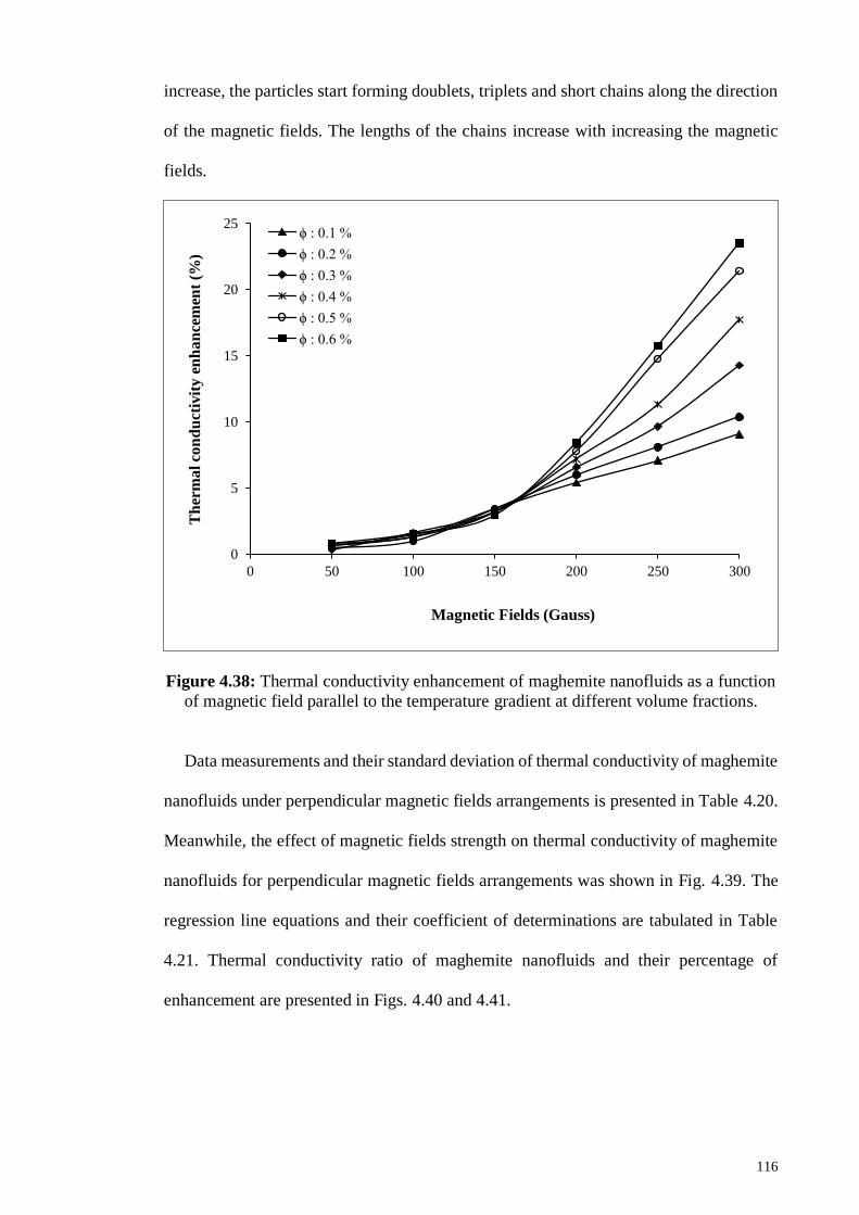
116
increase, the particles start forming doublets, triplets and short chains along the direction
of the magnetic fields. The lengths of the chains increase with increasing the magnetic
fields.
Figure 4.38: Thermal conductivity enhancement of maghemite nanofluids as a function
of magnetic field parallel to the temperature gradient at different volume fractions.
Data measurements and their standard deviation of thermal conductivity of maghemite
nanofluids under perpendicular magnetic fields arrangements is presented in Table 4.20.
Meanwhile, the effect of magnetic fields strength on thermal conductivity of maghemite
nanofluids for perpendicular magnetic fields arrangements was shown in Fig. 4.39. The
regression line equations and their coefficient of determinations are tabulated in Table
4.21. Thermal conductivity ratio of maghemite nanofluids and their percentage of
enhancement are presented in Figs. 4.40 and 4.41.
0
5
10
15
20
25
0 50 100 150 200 250 300
Th
erm
al
con
du
ctiv
ity e
nh
an
cem
ent
(%)
Magnetic Fields (Gauss)
ϕ : 0.1 %
ϕ : 0.2 %
ϕ : 0.3 %
ϕ : 0.4 %
ϕ : 0.5 %
ϕ : 0.6 %

117
Table 4.20: Thermal conductivity of maghemite nanofluids at
different perpendicular magnetic fields strength
Magnetic
fields strength
(Gauss)
Thermal conductivity (W/mK)
ϕ : 0.1 % ϕ : 0.2 % ϕ : 0.3 %
0 0.607 ± 0.0016 0.617 ± 0.0013 0.622 ± 0.0013
50 0.608 ± 0.0013 0.617 ± 0.0015 0.622 ± 0.0017
100 0.609 ± 0.0011 0.619 ± 0.0011 0.625 ± 0.0015
150 0.611 ± 0.0013 0.622 ± 0.0014 0.627 ± 0.0013
200 0.612 ± 0.0010 0.624 ± 0.0013 0.630 ± 0.0013
250 0.614 ± 0.0011 0.625 ± 0.0011 0.632 ± 0.0011
300 0.614 ± 0.0014 0.627 ± 0.0011 0.633 ± 0.0013
Magnetic
fields strength
(Gauss)
Thermal conductivity (W/mK)
ϕ : 0.4 % ϕ : 0.5 % ϕ : 0.6 %
0 0.627 ± 0.0016 0.631 ± 0.0016 0.643 ± 0.0016
50 0.629 ± 0.0015 0.633 ± 0.0015 0.644 ± 0.0013
100 0.632 ± 0.0016 0.636 ± 0.0013 0.645 ± 0.0011
150 0.635 ± 0.0013 0.639 ± 0.0011 0.648 ± 0.0013
200 0.637 ± 0.0015 0.641 ± 0.0015 0.651 ± 0.0014
250 0.641 ± 0.0018 0.645 ± 0.0016 0.654 ± 0.0016
300 0.643 ± 0.0014 0.650 ± 0.0011 0.656 ± 0.0013
Figure 4.39: Thermal conductivity of maghemite nanofluids at
different perpendicular magnetic fields strength
0.580
0.600
0.620
0.640
0.660
0.680
0.700
0 50 100 150 200 250 300
Th
erm
al
com
du
cti
vit
y (
W/m
K)
Magnetic fields (Gauss)
ϕ : 0.1 %
ϕ : 0.2 %
ϕ : 0.3 %
ϕ : 0.4 %
ϕ : 0.5 %
ϕ : 0.6 %
regression line

118
Table 4.21: Regression line equation of thermal conductivity of maghemite
nanofluids at different perpendicular magnetic fields strength.
Particle volume
fraction (%)
Equation line R2
0.1 Y = 3E-05X+0.6069 0.9759
0.2 Y = 4E-05X+0.6161 0.9705
0.3 Y = 4E-05X+0.6214 0.9849
0.4 Y = 6E-05X+0.6266 0.9948
0.5 Y = 6E-05X+0.6301 0.9804
0.6 Y = 5E-05X+0.6417 0.9708
It can be seen that the thermal conductivity of maghemite nanofluids is slightly
dependent on perpendicular magnetic fields. There is little epffect if the magnetic fields
are in position of a perpendicular direction to the samples. This can be explained that the
maghemite nanoparticles suspended in the solution will be aligning to the direction of the
magnetic fields. There has been very minor change in the thermal conductivity values,
irrespective the applied magnetic field strength and the volume fraction of the particles
as shown in Figs. 4.39 and 4.40. This can be explained that maghemite nanoparticles
suspended in the solution form chain-like aggregation structure were aligned to the
direction of magnetic fields (Shima et al., 2009). As a result, no chain alignment emerges
on the particles along the temperature gradient. Therefore, thermal conductivity of
nanofluids is weakly affected by perpendicular mode with maximum enhancement is only
2.69 %.
Without any external magnetic field, the magnetic moments of the scatterers are
oriented in the random direction. With the increase in magnetic field, the moments of the
magnetic particles start to align themselves along the direction of the magnetic fields.
Therefore, the observed enhancement of thermal conductivity is due to the effective
heat transport through chain-like aggregates of nanoparticles. Though the particle
aggregates in dispersions are fracted in nature, the aggregates formed are highly ordered
under an external magnetic field. This enhanced the conduction through percolation paths
that form parallel modes of conduction (Eapen et al., 2007).
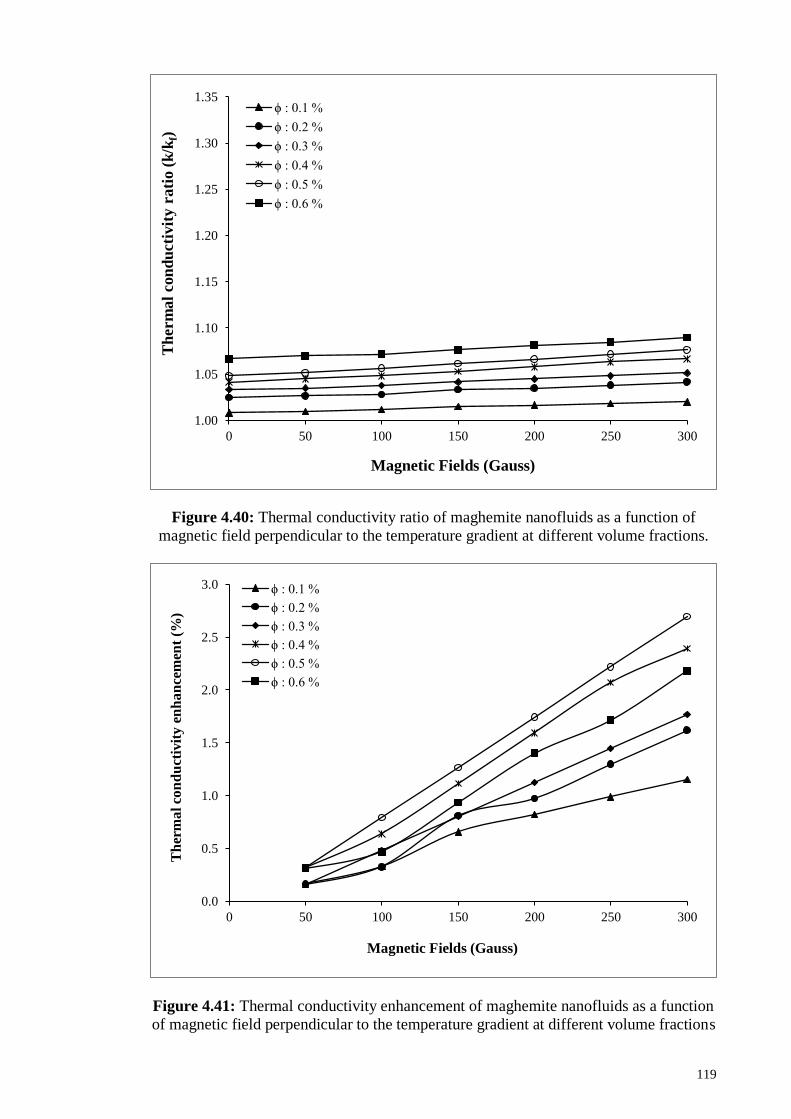
119
Figure 4.40: Thermal conductivity ratio of maghemite nanofluids as a function of
magnetic field perpendicular to the temperature gradient at different volume fractions.
Figure 4.41: Thermal conductivity enhancement of maghemite nanofluids as a function
of magnetic field perpendicular to the temperature gradient at different volume fractions
1.00
1.05
1.10
1.15
1.20
1.25
1.30
1.35
0 50 100 150 200 250 300
Th
erm
al
con
du
cti
vit
y r
ati
o (
k/k
f)
Magnetic Fields (Gauss)
ϕ : 0.1 %
ϕ : 0.2 %
ϕ : 0.3 %
ϕ : 0.4 %
ϕ : 0.5 %
ϕ : 0.6 %
0.0
0.5
1.0
1.5
2.0
2.5
3.0
0 50 100 150 200 250 300
Th
erm
al
con
du
ctiv
ity e
nh
an
cem
ent
(%)
Magnetic Fields (Gauss)
ϕ : 0.1 %
ϕ : 0.2 %
ϕ : 0.3 %
ϕ : 0.4 %
ϕ : 0.5 %
ϕ : 0.6 %

120
4.3.3.2 Kinematic Viscosity
Measurements and their standard deviation of kinematic viscosity of maghemite
nanofluids under parallel magnetic fields arrangements is presented in Table 4.22. The
effect of magnetic fields strength on kinematic viscosity of maghemite nanofluids for
parallel magnetic fields arrangements is shown in Fig. 4.42. The regression line equations
and their coefficient of determinations are tabulated in Table 4.23. Kinematic viscosity
ratio of maghemite nanofluids and their percentage of enhancement are presented in Figs.
4.43 and 4.44.
Table 4.22: Kinematic viscosity of maghemite nanofluids as a function of different
parallel magnetic fields strength at 25 oC for different particle volume fraction.
Magnetic
fields strength
(Gauss)
Kinematic viscosity (cst)
ϕ : 0.1 % ϕ : 0.2 % ϕ : 0.3 %
0 0.901 ± 0.0014 0.922 ± 0.0012 0.945 ± 0.0013
50 0.905 ± 0.0017 0.927 ± 0.0011 0.951 ± 0.0017
100 0.914 ± 0.0020 0.937 ± 0.0013 0.964 ± 0.0015
150 0.927 ± 0.0016 0.951 ± 0.0018 0.976 ± 0.0014
200 0.941 ± 0.0015 0.971 ± 0.0016 0.999 ± 0.0012
250 0.952 ± 0.0016 0.989 ± 0.0014 1.018 ± 0.0011
300 0.969 ± 0.0012 1.006 ± 0.0013 1.041 ± 0.0010
Magnetic
fields strength
(Gauss)
Kinematic viscosity (cst)
ϕ : 0.4 % ϕ : 0.5 % ϕ : 0.6 %
0 0.957 ± 0.0018 0.968 ± 0.0010 0.976 ± 0.0019
50 0.964 ± 0.0020 0.977 ± 0.0014 0.993 ± 0.0019
100 0.978 ± 0.0012 0.993 ± 0.0016 1.007 ± 0.0009
150 0.996 ± 0.0017 1.011 ± 0.0015 1.038 ± 0.0013
200 1.019 ± 0.0012 1.045 ± 0.0012 1.070 ± 0.0017
250 1.053 ± 0.0015 1.086 ± 0.0016 1.117 ± 0.0018
300 1.087 ± 0.0013 1.127 ± 0.0016 1.156 ± 0.0015

121
Figure 4.42: Kinematic viscosity of maghemite nanofluids as a function of different
parallel magnetic fields strength at 25 oC for different particle volume fractions.
Table 4.23: Regression line equation of kinematic viscosity of maghemite
nanofluids at different parallel magnetic fields strength
Particle volume
fraction (%)
Equation line R2
0.1 Y = 4E-07X2 +0.0001X+0.8996 0.9964
0.2 Y = 5E-07X2 +1E-04X+0.9205 0.9964
0.3 Y = 7E-06X2+ 0.0001X+0.9440 0.9979
0.4 Y = 1E-06X2 +8E-05X+0.9570 0.9995
0.5 Y = 2E-06X2 +8E-05X+0.9684 0.9987
0.6 Y = 1E-06X2 +0.0002X+0.9763 0.9978
It can be seen that the kinematic viscosity of maghemite nanofluids is increased with
increasing of magnetic fields strength at any particle volume fraction. In the presence of
magnetic field, the viscosity of the nanofluid become strongly anisotropic due to
nanoparticle structure that alter the transport properties.
0.880
0.920
0.960
1.000
1.040
1.080
1.120
1.160
0 50 100 150 200 250 300
Kin
em
ati
c v
iscosi
ty (
cst
)
Magnetic fields (Gauss)
ϕ : 0.1 %
ϕ : 0.2 %
ϕ : 0.3 %
ϕ : 0.4 %
ϕ : 0.5 %
ϕ : 0.6 %
regression line

122
Figure 4.43: Kinematic viscosity ratio of maghemite nanofluids as a function of
different parallel magnetic fields strength at 25 oC for different particle volume fractions
Figure 4.44: Kinematic viscosity enhancement of maghemite nanofluids as
a function of different parallel magnetic fields strength at 25 oC
for different particle volume fractions.
1.00
1.05
1.10
1.15
1.20
1.25
1.30
1.35
0 50 100 150 200 250 300
Kin
ema
tic
vis
cosi
ty r
ati
o (
µ/µ
f)
Magnetic Fields (Gauss)
ϕ : 0.1 %
ϕ : 0.2 %
ϕ : 0.3 %
ϕ : 0.4 %
ϕ : 0.5 %
ϕ : 0.6 %
0
5
10
15
20
0 50 100 150 200 250 300
Kin
ema
tic
vis
cosi
ty e
nh
an
cem
ent
(%)
Magnetic Fields (Gauss)
ϕ : 0.1 %
ϕ : 0.2 %
ϕ : 0.3 %
ϕ : 0.4 %
ϕ : 0.5 %
ϕ : 0.6 %

123
Measurements and their standard deviation of kinematic viscosity of maghemite
nanofluids under perpendicular magnetic fields arrangements is presented in Table 4.24.
The effect of magnetic fields strength on kinematic viscosity of maghemite nanofluids for
parallel magnetic fields arrangements is shown in Fig. 4.45. The regression line equations
and their coefficient of determinations are tabulated in Table 4.25. Kinematic viscosity
ratio of maghemite nanofluids and their percentage of enhancement are presented in Figs.
4.46 and 4.47.
Table 4.24: Kinematic viscosity of maghemite nanofluids
at different perpendicular magnetic fields strength
Magnetic
fields strength
(Gauss)
Kinematic viscosity (cst)
ϕ : 0.1 % ϕ : 0.2 % ϕ : 0.3 %
0 0.901 ± 0.0014 0.922 ± 0.0012 0.945 ± 0.0013
50 0.906 ± 0.0015 0.926 ± 0.0013 0.952 ± 0.0015
100 0.912 ± 0.0013 0.934 ± 0.0017 0.961 ± 0.0010
150 0.920 ± 0.0012 0.942 ± 0.0018 0.969 ± 0.0016
200 0.928 ± 0.0022 0.957 ± 0.0017 0.978 ± 0.0010
250 0.938 ± 0.0021 0.972 ± 0.0012 0.989 ± 0.0014
300 0.955 ± 0.0021 0.988 ± 0.0014 1.010 ± 0.0014
Magnetic
fields strength
(Gauss)
Kinematic viscosity (cst)
ϕ : 0.4 % ϕ : 0.5 % ϕ : 0.6 %
0 0.957 ± 0.0018 0.968 ± 0.0010 0.976 ± 0.0019
50 0.964 ± 0.0015 0.975 ± 0.0015 0.985 ± 0.0021
100 0.972 ± 0.0011 0.983 ± 0.0020 0.997 ± 0.0013
150 0.984 ± 0.0010 0.998 ± 0.0016 1.014 ± 0.0015
200 1.002 ± 0.0016 1.021 ± 0.0019 1.036 ± 0.0017
250 1.022 ± 0.0012 1.051 ± 0.0018 1.073 ± 0.0013
300 1.045 ± 0.0021 1.078 ± 0.0014 1.102 ± 0.0014
It can be seen that the kinematic viscosity of maghemite nanofluids at any particle
volume fraction is increased with magnetic fields strength. For diluted maghemite
nanofluids with noninteracting particles, the Brownian motion of particles is hindered by
magnetic fields, resulting in the increase of kinematic viscosity. In the other case, the
interactions between particles and particularly the cluster formation will further increase
the viscosity.

124
Figure 4.45: Kinematic viscosity of maghemite nanofluids at different
perpendicular magnetic fields strength at 25 oC.
Table 4.25: Regression line equation of kinematic viscosity of maghemite
nanofluids at different perpendicular magnetic fields strength.
Particle volume
fraction (%)
Equation line R2
0.1 Y = 4E-07X2 +1E-04X+0.9017 0.9958
0.2 Y = 5E-07X2 +7E-05X+0.9217 0.9986
0.3 Y = 4E-07X2 +9E-05X+0.9462 0.9912
0.4 Y = 7E-07X2 +8E-05X+0.9574 0.9996
0.5 Y = 1E-06X2 +5E-05X+0.9683 0.9980
0.6 Y = 1E-06X2 +9E-05X+0.9766 0.9974
When maghemite nanofluids were subjected to both perpendicular and parallel
magnetic fields arrangement, the particle chains along the direction of magnetic fields
blocks the flow channel of the maghemite nanofluids, resulted in higher friction force
along the flow of maghemite nanofluids. This phenomenon enhances the kinematic
viscosity of maghemite nanofluids.
0.880
0.920
0.960
1.000
1.040
1.080
1.120
1.160
0 50 100 150 200 250 300
Kin
em
ati
c v
iscosi
ty (
cst
)
Magnetic fields (Gauss)
ϕ : 0.1 %
ϕ : 0.2 %
ϕ : 0.3 %
ϕ : 0.4 %
ϕ : 0.5 %
ϕ : 0.6 %
regression line

125
It can also be seen that the kinematic viscosity of maghemite nanofluids are slightly
higher in parallel magnetic fields arrangement compared to perpendicular magnetic fields
arrangement.
The highest enhancement of kinematic viscosity of maghemite nanofluids at
perpendicular and parallel arrangement are 12.91 % and 18.44 %, respectively which
obtained at magnetic fields strength of 300 Gauss and particle volume fraction of 0.6 %.
Figure 4.46: Kinematic viscosity ratio of maghemite nanofluids as a function of
magnetic field perpendicular to the temperature gradient at different volume fractions.
1.00
1.05
1.10
1.15
1.20
1.25
1.30
1.35
0 50 100 150 200 250 300
Kin
ema
tic
vis
cosi
ty r
ati
o (
µ/µ
f)
Magnetic Fields (Gauss)
ϕ : 0.1 %
ϕ : 0.2 %
ϕ : 0.3 %
ϕ : 0.4 %
ϕ : 0.5 %
ϕ : 0.6 %
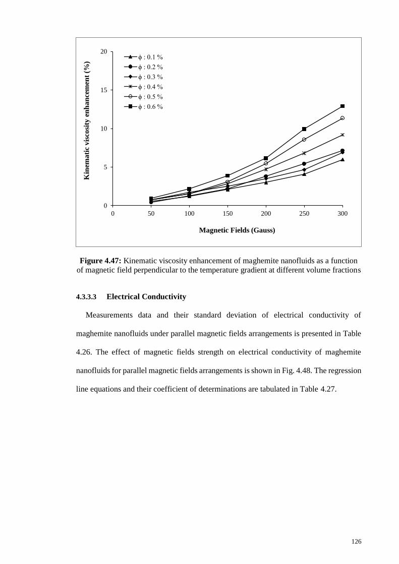
126
Figure 4.47: Kinematic viscosity enhancement of maghemite nanofluids as a function
of magnetic field perpendicular to the temperature gradient at different volume fractions
4.3.3.3 Electrical Conductivity
Measurements data and their standard deviation of electrical conductivity of
maghemite nanofluids under parallel magnetic fields arrangements is presented in Table
4.26. The effect of magnetic fields strength on electrical conductivity of maghemite
nanofluids for parallel magnetic fields arrangements is shown in Fig. 4.48. The regression
line equations and their coefficient of determinations are tabulated in Table 4.27.
0
5
10
15
20
0 50 100 150 200 250 300
Kin
ema
tic
vis
cosi
ty e
nh
an
cem
ent
(%)
Magnetic Fields (Gauss)
ϕ : 0.1 %
ϕ : 0.2 %
ϕ : 0.3 %
ϕ : 0.4 %
ϕ : 0.5 %
ϕ : 0.6 %

127
Table 4.26: Electrical conductivity of maghemite nanofluids at
different parallel magnetic fields strength
Magnetic
fields strength
(Gauss)
Electrical Conductivity (mS/cm)
ϕ : 0.1 % ϕ : 0.2 % ϕ : 0.3 %
0 1.011 ± 0.0013 2.019 ± 0.0013 3.160 ± 0.0014
50 1.011 ± 0.0009 2.020 ± 0.0013 3.161 ± 0.0009
100 1.012 ± 0.0014 2.020 ± 0.0015 3.161 ± 0.0010
150 1.013 ± 0.0011 2.021 ± 0.0009 3.162 ± 0.0013
200 1.013 ± 0.0011 2.021 ± 0.0013 3.162 ± 0.0011
250 1.014 ± 0.0016 2.022 ± 0.0013 3.163 ± 0.0014
300 1.015 ± 0.0008 2.023 ± 0.0009 3.164 ± 0.0012
Magnetic
fields strength
(Gauss)
Electrical Conductivity (mS/cm)
ϕ : 0.4 % ϕ : 0.5 % ϕ : 0.6 %
0 4.109 ± 0.0010 4.994 ± 0.0013 6.624 ± 0.0013
50 4.113 ± 0.0013 4.996 ± 0.0013 6.627 ± 0.0010
100 4.113 ± 0.0008 4.998 ± 0.0010 6.630 ± 0.0009
150 4.115 ± 0.0011 5.002 ± 0.0009 6.631 ± 0.0013
200 4.116 ± 0.0013 5.003 ± 0.0015 6.632 ± 0.0013
250 4.117 ± 0.0009 5.004 ± 0.0014 6.634 ± 0.0013
300 4.119 ± 0.0008 5.005 ± 0.0009 6.635 ± 0.0010
Figure 4.48: Electrical conductivity of maghemite nanofluids as a function of magnetic
field parallel to the temperature gradient at different volume fractions.
0.0
1.0
2.0
3.0
4.0
5.0
6.0
7.0
8.0
0 50 100 150 200 250 300
Ele
ctr
ical C
on
du
cti
vit
y (
mS
/cm
)
Magnetic fields (Gauss)
ϕ : 0.1 % ϕ : 0.2 %ϕ : 0.3 % ϕ : 0.4 %ϕ : 0.5 % ϕ : 0.6 %regression line

128
Table 4.27: Regression line equation of electrical conductivity of maghemite
nanofluids at different parallel magnetic fields strength.
Particle volume
fraction (%)
Equation line R2
0.1 Y = 1E-5X+1.0107 0.9601
0.2 Y = 1E-5X+2.019 0.9507
0.3 Y = 1E-5X+3.16 0.9507
0.4 Y = 3E-5X+4.1102 0.9423
0.5 Y = 4E-5X+4.9945 0.9517
0.6 Y = 4E-5X+6.6252 0.9558
It can be seen that the electrical conductivity of maghemite nanofluids are independent
of the magnetic fields strength at any particle volume fraction. This can be explained that
the electrical conductivity of nanofluids is related to the ability of charged particles (ions)
in the suspensions to carry the charges (electrons) towards respective electrode when the
electrical potential is applied. In nanofluids, the dispersed nanoparticles in a base fluids
get charged due to the formation of electrical double layers around the particle surface.
These nanoparticles along with EDL move towards oppositely charged electrode when
the potential is applied. This EDL formation depends on the surface charge (pH), size and
particle volume fraction and ionic concentration in base fluids. Thus the electrophoretic
mobility of charged particles determines the electrical conductivity of nanofluids
(Sarojini et al., 2013).
Without any external magnetic field, the magnetic moments of the scatterers are
oriented in the random direction. With the increase in magnetic field, the moments of the
magnetic particles start to align themselves along the direction of the magnetic fields.
However, the surface charge of the particles is remained with the effect of magnetic fields.
Hence, the electrical conductivity of maghemite nanofluids remain stable at any particular
concentrations.
Measurements data and their standard deviation of electrical conductivity of
maghemite nanofluids under perpendicular magnetic fields arrangements is presented in
Table 4.28. The effect of magnetic fields strength on electrical conductivity of maghemite

129
nanofluids for perpendicular magnetic fields arrangements was shown in Fig. 4.49. The
regression line equations and their coefficient of determinations are tabulated in Table
4.29.
Table 4.28: Electrical conductivity of maghemite nanofluids at different
perpendicular magnetic fields strength
Magnetic
fields strength
(Gauss)
Electrical Conductivity (mS/cm)
ϕ : 0.1 % ϕ : 0.2 % ϕ : 0.3 %
0 1.013 ± 0.0011 2.019 ± 0.0008 3.130 ± 0.0011
50 1.016 ± 0.0010 2.022 ± 0.0009 3.133 ± 0.0010
100 1.018 ± 0.0013 2.023 ± 0.0010 3.135 ± 0.0013
150 1.020 ± 0.0010 2.024 ± 0.0008 3.137 ± 0.0015
200 1.021 ± 0.0011 2.025 ± 0.0010 3.139 ± 0.0013
250 1.022 ± 0.0013 2.027 ± 0.0009 3.139 ± 0.0010
300 1.023 ± 0.0011 2.028 ± 0.0009 3.140 ± 0.0011
Magnetic
fields strength
(Gauss)
Electrical Conductivity (mS/cm)
ϕ : 0.4 % ϕ : 0.5 % ϕ : 0.6 %
0 4.118 ± 0.0011 5.008 ± 0.0011 6.628 ± 0.0009
50 4.120 ± 0.0010 5.011 ± 0.0010 6.630 ± 0.0011
100 4.121 ± 0.0008 5.012 ± 0.0013 6.631 ± 0.0013
150 4.123 ± 0.0010 5.014 ± 0.0010 6.633 ± 0.0011
200 4.123 ± 0.0015 5.015 ± 0.0008 6.633 ± 0.0013
250 4.124 ± 0.0009 5.016 ± 0.0011 6.634 ± 0.0008
300 4.125 ± 0.0010 5.017 ± 0.0008 6.635 ± 0.0009
It can also be observed that the magnetic fields strength does not affect the electrical
conductivity of maghemite nanofluids at perpendicular arrangement of magnetic fields.
According to EDL theory, since the charged nanoparticles are electrically conducting
material, the electrical conductivity may still increase due to establishment of short
conducting paths by aggregate contact of the solid materials. According to this
assumption, the EDL effects are very small and insignificant, and, therefore, the
electrophoretic effects may be also unimportant (Washabaugh et al., 1996).
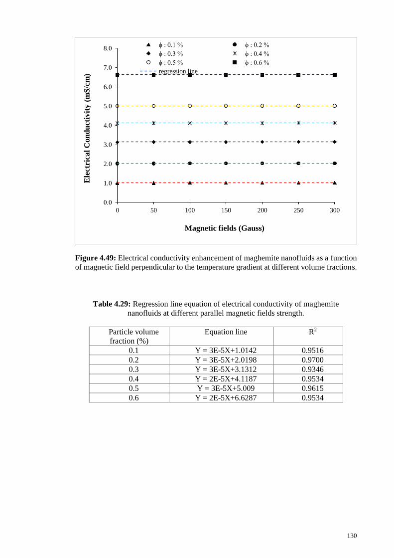
130
Figure 4.49: Electrical conductivity enhancement of maghemite nanofluids as a function
of magnetic field perpendicular to the temperature gradient at different volume fractions.
Table 4.29: Regression line equation of electrical conductivity of maghemite
nanofluids at different parallel magnetic fields strength.
Particle volume
fraction (%)
Equation line R2
0.1 Y = 3E-5X+1.0142 0.9516
0.2 Y = 3E-5X+2.0198 0.9700
0.3 Y = 3E-5X+3.1312 0.9346
0.4 Y = 2E-5X+4.1187 0.9534
0.5 Y = 3E-5X+5.009 0.9615
0.6 Y = 2E-5X+6.6287 0.9534
0.0
1.0
2.0
3.0
4.0
5.0
6.0
7.0
8.0
0 50 100 150 200 250 300
Ele
ctr
ical
Con
du
cti
vit
y (
mS
/cm
)
Magnetic fields (Gauss)
ϕ : 0.1 % ϕ : 0.2 %
ϕ : 0.3 % ϕ : 0.4 %
ϕ : 0.5 % ϕ : 0.6 %
regression line
131
CONCLUSIONS AND RECOMENDATIONS
This chapter describes the conclusions of the synthesis, characterization and
thermophysical properties of maghemite nanofluids with and without magnetic fields
effect and recommendations for future research.
5.1 Conclusions
Stable maghemite nanoparticles have been successfully synthesized using a chemical
coprecipitation method with the effect of nitric acid concentrations as an oxidizing agent.
The pattern obtained from XRD results confirm that the particles are maghemite. The
morphology of maghemite nanoparticles are spherical. The maghemite nanoparticles
show superparamagnetic behavior with decreased magnetization values at the increasing
concentration of nitric acid concentration. With this behavior, the maghemite
nanoparticles can be controlled with external magnetic fields. Thermal stability of
maghemite nanoparticles show a two steps weight loss behavior. TGA measurement
showed that the stability temperature decreases with the increasing concentration of nitric
acid. The temperature stability is achieved earlier at the smaller particle size. DLS
measurement showed that the hydrodynamic particle sizes decrease with the increasing
concentration of nitric acid. The zeta potential values decrease with the increasing
concentration of nitric acid. The increasing concentration of nitric acid in synthesis of
maghemite nanoparticles produced smaller size particles, lower magnetization, better
thermal stability and more stable maghemite nanofluids. It can be concluded that the best
result from synthesis parameter is using 10 M nitric acid concentration.
The environmental play a significant role in the stability of the suspension. The
maghemite nanofluids are remain stable with the effect of time of storage. The
suspensions remain stable after eight months of storage.
132
The particle volume fraction has significant effect to the enhancement of the
thermophysical properties of maghemite nanofluids. The thermal conductivity of
maghemite nanofluids linearly increases with the increasing of particle volume fraction.
The kinematic viscosity of maghemite nanofluids linearly increases with increasing of
particle volume fraction. The electrical conductivity of maghemite nanofluids is
signicantly increase with the increasing of particle volume fraction.
The temperature of the solution also effects the properties of thermophysical properties
of maghemite nanofluids. The temperature is significantly effects of thermal conductivity
by randomly increase the molecule movement in the suspension. Hence, thermal
conductivity of maghemite nanofluids nonlinearly increase with the increasing of
temperature. The kinematic viscosity of maghemite nanofluids nonlinearly decrease with
the increasing of temperature of solutions due to weakening of inter-particle and inter-
molecular adhesion forces hence accelerate the movement of the particles in liquids. The
electrical conductivity of maghemite nanofluids linearly increases with the increasing of
temperature.
The effect of external magnetic fields on the thermophysical properties of maghemite
nanofluids is significant. The data show that thermal conductivity of maghemite
nanofluids increases with the increasing of the strength of magnetic fields for parallel and
perpendicular magnetic fields arrangements. The parallel arrangement has significant
enhancement compared to perpendicular arrangement. The kinematic viscosity of
maghemite nanofluids also increase with increasing of magnetic fields strength for both
parallel and perpendicular arrangements. The enhancement of kinematic viscosity of
maghemite nanofluids for parallel arrangement is higher than perpendicular arrangement.
The electrical conductivity of maghemite nanofluids are not influenced by the increasing
of magnetic fields strength for both parallel and perpendicular arrangements.

133
5.2 Recommendations
In this study maghemite nanoparticles have been synthesized using chemical co-
precipitation method. Preparation of maghemite nanofluids is conducted by disperse a
certain amount of maghemite nanoparticles in water as base fluids. The thermophysical
properties is studied at the effect of particle volume fraction, temperatures and magnetic
fields. Some considerations and recommendations can be suggested to further
investigated of the unique maghemite nanofluids.
1. The maghemite nanoparticles were synthesized at different nitric acid concentration.
The results show that stable maghemite nanoparticle have been synthesized. There are
several factors that influenced the synthesis of maghemite nanoparticles by co-
precipitation methods, such as temperature, concentration ratio, and reaction time. It
is suggested to further investigate those effect to get more detail results.
2. The stability of nanofluids is strongly depend on the pH of the solution. In this study,
the pH of maghemite nanofluids is 3.60. We did not put any surfactant for the stability
study to these nanofluids. Therefore, in order to further investigate the stability of
maghemite nanofluids in various pHs, it suggested to evaluate the effect of surfactant
on the stability of maghemite nanofluids.
3. The thermophysical properties are important parameters in the application of
maghemite nanofluids. Several parameters such as thermal conductivity, viscosity, and
electrical conductivity have been studied in various effect such as particle volume
fraction, temperature, and magnetic fields strength. However, there are many other
parameters and effects which are not yet been explored. Hence, further investigations
are required to enrich physical properties data for maghemite nanofluids.
4. This study has not been considered the model development for the formulation of
thermophysical properties of maghemite nanofluids. This is needed in order to predict

134
the properties of maghemite nanofluids in the application processes. So, the
development of the model is required in the further study.

135
REFERENCES
Abareshi, M., Goharshadi, E. K., Zebarjad, S. M., Fadafan, H. K., & Youssefi, A. (2010).
Fabrication, characterization and measurement of thermal conductivity of Fe3O4
nanofluids. Journal of Magnetism and Magnetic Materials, 322(24), 3895-3901.
Abbas, M., Islam, M. N., Rao, B. P., Abdel-Hamed, M. O., & Kim, C. (2015). Facile one-
pot chemical approach for synthesis of monodisperse chain-like
superparamagnetic maghemite (γ-Fe2O3) nanoparticles. Journal of Industrial and
Engineering Chemistry, 31, 43-46.
Ali, K., Sarfraz, A. K., Mirza, I. M., Bahadur, A., Iqbal, S., & ul Haq, A. (2015).
Preparation of superparamagnetic maghemite (γ-Fe2O3) nanoparticles by wet
chemical route and investigation of their magnetic and dielectric properties.
Current Applied Physics, 15(8), 925-929.
Alsaady, M., Fu, R., Li, B., Boukhanouf, R., & Yan, Y. (2015). Thermo-physical
properties and thermo-magnetic convection of ferrofluid. Applied Thermal
Engineering, 88, 14-21.
Asuha, S., Suyala, B., Siqintana, X., & Zhao, S. (2011). Direct synthesis of Fe3O4
nanopowder by thermal decomposition of Fe-urea complex and its properties.
Journal of Alloys and Compounds, 509(6), 2870-2873.
Azmi, W. H., Sharma, K. V., Mamat, R., Najafi, G., & Mohamad, M. S. (2016). The
enhancement of effective thermal conductivity and effective dynamic viscosity of
nanofluids – A review. Renewable and Sustainable Energy Reviews, 53, 1046-
1058.
Babita, Sharma, S. K., & Gupta, S. M. (2016). Preparation and evaluation of stable
nanofluids for heat transfer application: A review. Experimental Thermal and
Fluid Science, 79, 202-212.
Baby, T. T., & Ramaprabhu, S. (2010). Investigation of thermal and electrical
conductivity of graphene based nanofluids. Journal of Applied Physics, 108(12),
124308.
Bagheli, S., Fadafan, H. K., Orimi, R. L., & Ghaemi, M. (2015). Synthesis and
experimental investigation of the electrical conductivity of water based magnetite
nanofluids. Powder Technology, 274, 426-430.
Bailar Jr, J. C., & Auten, R. W. (1934). The stereochemistry of complex inorganic
compounds. I. The Walden inversion as exhibited by diethylenediaminocobaltic
compounds. Journal of the American Chemical Society, 56(4), 774-776.
Batchelor, G. (1977). The effect of Brownian motion on the bulk stress in a suspension
of spherical particles. Journal of Fluid Mechanics, 83(01), 97-117.
Bee, A., Massart, R., & Neveu, S. (1995). Synthesis of Very Fine Maghemite Particles.
Journal of Magnetism and Magnetic Materials, 149(1-2), 6-9.
Behdadfar, B., Kermanpur, A., Sadeghi-Aliabadi, H., Morales, M. D., & Mozaffari, M.
(2012). Synthesis of aqueous ferrofluids of ZnxFe3-xO4 nanoparticles by citric
136
acid assisted hydrothermal-reduction route for magnetic hyperthermia
applications. Journal of Magnetism and Magnetic Materials, 324(14), 2211-2217.
Blasiak, B., van Veggel, F. C., & Tomanek, B. (2013). Applications of nanoparticles for
MRI cancer diagnosis and therapy. Journal of Nanomaterials, 2013, 12.
Blums, E. (2002). Heat and mass transfer phenomena. Journal of Magnetism and
Magnetic Materials, 252(0), 189-193.
Brinkman, H. (1952). The viscosity of concentrated suspensions and solutions. The
Journal of Chemical Physics, 20(4), 571-571.
Bruggeman, D. (1935). Dielectric constant and conductivity of mixtures of isotropic
materials. Ann Phys (Leipzig), 24, 636-679.
Cabuil, V., Neveu, S., & Rosensweig, R. (1993). Introduction to the magnetic fluids
bibliography. Journal of Magnetism and Magnetic Materials, 122(1), 437-438.
Caparrós, C., Benelmekki, M., Martins, P. M., Xuriguera, E., Silva, C. J. R., Martinez, L.
M., & Lanceros-Méndez, S. (2012). Hydrothermal assisted synthesis of iron
oxide-based magnetic silica spheres and their performance in magnetophoretic
water purification. Materials Chemistry and Physics, 135(2–3), 510-517.
Carp, M., Müller, R., Draghiciu, L., Voicu, R., & Danila, M. (2011). Characterization of
microdevices for ferrous chloride separation for biosensing applications. Sensors
and Actuators A: Physical, 171(1), 26-33.
Casula, M. F., Corrias, A., Arosio, P., Lascialfari, A., Sen, T., Floris, P., & Bruce, I. J.
(2011). Design of water-based ferrofluids as contrast agents for magnetic
resonance imaging. Journal of Colloid and Interface Science, 357(1), 50-55.
Charles, S. W. (2002). The preparation of magnetic fluids Ferrofluids (pp. 3-18): Berlin,
Springer.
Chaudhury, M. K. (2003). Complex fluids: Spread the word about nanofluids. Nature,
423(6936), 131-132.
Chin, A. B., & Yaacob, I. I. (2007). Synthesis and characterization of magnetic iron oxide
nanoparticles via w/o microemulsion and Massart's procedure. Journal of
materials processing technology, 191(1), 235-237.
Choi, S.-S. (1998). Nanofluid technology: current status and future research: Argonne
National Lab., IL (US).
Choi, S. U., Xu, X., Keblinski, P., & Yu, W. (2002). Nanofluids can take the heat. Paper
presented at the DOE/BES Symposium on Energy Engineering Sciences.
Choi, S. U., Zhang, Z. G., & Keblinski, P. (2004). Nanofluids Encyclopedia of
Nanoscience and Nanotechnology (Vol. 6, pp. 757-773): American Scientific
Publishers.
Chol, S. (1995). Enhancing thermal conductivity of fluids with nanoparticles. ASME-
Publications-Fed, 231, 99-106.
137
Chopkar, M., Das, P. K., & Manna, I. (2006). Synthesis and characterization of nanofluid
for advanced heat transfer applications. Scripta Materialia, 55(6), 549-552.
Chopkar, M., Kumar, S., Bhandari, D., Das, P. K., & Manna, I. (2007). Development and
characterization of Al2Cu and Ag2Al nanoparticle dispersed water and ethylene
glycol based nanofluid. Materials Science and Engineering: B, 139(2), 141-148.
Cruz, R. C., Reinshagen, J., Oberacker, R., Segadães, A. M., & Hoffmann, M. J. (2005).
Electrical conductivity and stability of concentrated aqueous alumina
suspensions. Journal of Colloid and Interface Science, 286(2), 579-588.
Cuny, L., Herrling, M. P., Guthausen, G., Horn, H., & Delay, M. (2015). Magnetic
resonance imaging reveals detailed spatial and temporal distribution of iron-based
nanoparticles transported through water-saturated porous media. Journal of
Contaminant Hydrology, 182, 51-62.
Dibaji, S. A. R., Al-Rjoub, M. F., Myers, M. R., & Banerjee, R. K. (2013). Enhanced
Heat Transfer and Thermal Dose Using Magnetic Nanoparticles During HIFU
Thermal Ablation—An In-Vitro Study. Journal of Nanotechnology in
Engineering and Medicine, 4(4), 040902.
Dobnikar, J., Haložan, D., Brumen, M., Von Grünberg, H.-H., & Rzehak, R. (2004).
Poisson–Boltzmann Brownian dynamics of charged colloids in suspension.
Computer Physics Communications, 159(2), 73-92.
Dong, M., Shen, L., Wang, H., Wang, H., & Miao, J. (2013). Investigation on the
electrical conductivity of transformer oil-based AlN nanofluid. Journal of
Nanomaterials, 2013, 164.
Eapen, J., Williams, W. C., Buongiorno, J., Hu, L.-w., Yip, S., Rusconi, R., & Piazza, R.
(2007). Mean-field versus microconvection effects in nanofluid thermal
conduction. Physical Review Letters, 99(9), 095901.
Eastman, J. A., Phillpot, S., Choi, S., & Keblinski, P. (2004). Thermal transport in
nanofluids 1. Annu. Rev. Mater. Res., 34, 219-246.
Eggers, J. R., & Kabelac, S. (2016). Nanofluids revisited. Applied Thermal Engineering,
106, 1114-1126.
Einstein, A. (1906). Eine neue bestimmung der moleküldimensionen. Annalen der
Physik, 324(2), 289-306.
Evans, W., Prasher, R., Fish, J., Meakin, P., Phelan, P., & Keblinski, P. (2008). Effect of
aggregation and interfacial thermal resistance on thermal conductivity of
nanocomposites and colloidal nanofluids. International Journal of Heat and Mass
Transfer, 51(5), 1431-1438.
Fang, F., & Zhang, Y. (2005). DC electrical conductivity of Au nanoparticle/chloroform
and toluene suspensions. Journal of materials science, 40(11), 2979-2980.
Fleet, M. E. (1986). The structure of magnetite: Symmetry of cubic spinels. Journal of
Solid State Chemistry, 62(1), 75-82.
138
Fu, H. L., & Gao, L. (2012). Effect of interfacial nanolayer on thermophoresis in
nanofluids. International Journal of Thermal Sciences, 61(0), 61-66.
Fultz, B., & Howe, J. M. (2012). Transmission electron microscopy and diffractometry
of materials: Springer Science & Business Media.
Galindo, R., Dector, A., Arriaga, L., Gutiérrez, S., & Herrasti, P. (2012). Maghemite as a
catalyst for glucose oxidation in a microfluidic fuel cell. Journal of
Electroanalytical Chemistry, 671, 38-43.
Ganguly, S., Sikdar, S., & Basu, S. (2009). Experimental investigation of the effective
electrical conductivity of aluminum oxide nanofluids. Powder Technology,
196(3), 326-330.
Gao, L., Zhou, X., & Ding, Y. (2007). Effective thermal and electrical conductivity of
carbon nanotube composites. Chemical Physics Letters, 434(4), 297-300.
Gavili, A., Zabihi, F., Isfahani, T. D., & Sabbaghzadeh, J. (2012). The thermal
conductivity of water base ferrofluids under magnetic field. Experimental
Thermal and Fluid Science, 41, 94-98.
Genc, S., & Derin, B. (2014). Synthesis and rheology of ferrofluids: a review. Current
Opinion in Chemical Engineering, 3, 118-124.
Ghadimi, A., Saidur, R., & Metselaar, H. (2011). A review of nanofluid stability
properties and characterization in stationary conditions. International Journal of
Heat and Mass Transfer, 54(17), 4051-4068.
Glory, J., Bonetti, M., Helezen, M., Mayne-L’Hermite, M., & Reynaud, C. (2008).
Thermal and electrical conductivities of water-based nanofluids prepared with
long multiwalled carbon nanotubes. Journal of Applied Physics, 103(9), 094309.
Godson, L., Raja, B., Mohan Lal, D., & Wongwises, S. (2010). Enhancement of heat
transfer using nanofluids—An overview. Renewable and Sustainable Energy
Reviews, 14(2), 629-641.
Gonçalves, J. R. (2016). The Soil and Groundwater Remediation with Zero Valent Iron
Nanoparticles. Procedia Engineering, 143, 1268-1275.
Goshayeshi, H. R., Goodarzi, M., Safaei, M. R., & Dahari, M. Experimental Study on the
Effect of Inclination Angle on Heat Transfer Enhancement of a Ferrofluid in a
Closed Loop Oscillating Heat Pipe under Magnetic Field. Experimental Thermal
and Fluid Science.
Gupte, S. K., Advani, S. G., & Huq, P. (1995). Role of micro-convection due to non-
affine motion of particles in a mono-disperse suspension. International Journal of
Heat and Mass Transfer, 38(16), 2945-2958.
Hamilton, R., & Crosser, O. (1962). Thermal conductivity of heterogeneous two-
component systems. Industrial & Engineering chemistry fundamentals, 1(3), 187-
191.
Haynes, W. M. (2013). CRC handbook of chemistry and physics: Londan, CRC press.

139
Herrmann, I., Schlegel, A., Graf, R., Stark, W., & Beck-Schimmer, B. (2015). Magnetic
separation-based blood purification: a promising new approach for the removal of
disease-causing compounds. Journal of nanobiotechnology, 13(1), 49.
Hong, T.-K., Yang, H.-S., & Choi, C. (2005). Study of the enhanced thermal conductivity
of Fe nanofluids. Journal of Applied Physics, 97(6), 064311.
Hsieh, T.-H., Ho, K.-S., Bi, X., Han, Y.-K., Chen, Z.-L., Hsu, C.-H., & Chang, Y.-C.
(2009). Synthesis and electromagnetic properties of polyaniline-coated
silica/maghemite nanoparticles. European Polymer Journal, 45(3), 613-620.
Huang, C., Neoh, K. G., Wang, L., Kang, E.-T., & Shuter, B. (2010). Magnetic
nanoparticles for magnetic resonance imaging: modulation of macrophage uptake
by controlled PEGylation of the surface coating. Journal of Materials Chemistry,
20(39), 8512-8520.
Huang, J., Wang, X., Long, Q., Wen, X., Zhou, Y., & Li, L. (2009). Influence of pH on
the stability characteristics of nanofluids. Paper presented at the Photonics and
Optoelectronics, 2009. SOPO 2009. Wuhan, China.
Huminic, G., Huminic, A., Morjan, I., & Dumitrache, F. (2011). Experimental study of
the thermal performance of thermosyphon heat pipe using iron oxide
nanoparticles. International Journal of Heat and Mass Transfer, 54(1), 656-661.
Hunter, R. J. (2013). Zeta potential in colloid science: principles and applications (Vol.
2): London, Academic press limited.
Hwang, Y., Lee, J.-K., Lee, J.-K., Jeong, Y.-M., Cheong, S.-i., Ahn, Y.-C., & Kim, S. H.
(2008). Production and dispersion stability of nanoparticles in nanofluids. Powder
Technology, 186(2), 145-153.
Hwang, Y., Lee, J. K., Lee, C. H., Jung, Y. M., Cheong, S. I., Lee, C. G., . . . Jang, S. P.
(2007). Stability and thermal conductivity characteristics of nanofluids.
Thermochimica Acta, 455(1–2), 70-74.
İlhan, B., Kurt, M., & Ertürk, H. (2016). Experimental investigation of heat transfer
enhancement and viscosity change of hBN nanofluids. Experimental Thermal and
Fluid Science, 77, 272-283.
Jakubovics, J. P., & Jakubovics, J. (1994). Magnetism and magnetic materials: Institute
of Materials.
Jang, S. P., & Choi, S. U. (2004). Role of Brownian motion in the enhanced thermal
conductivity of nanofluids. Applied Physics Letters, 84(21), 4316-4318.
Johnson, G., Benveniste, H., Black, R., Hedlund, L., Maronpot, R., & Smith, B. (1993).
Histology by magnetic resonance microscopy. Magnetic resonance quarterly,
9(1), 1-30.
Keblinski, P., Phillpot, S., Choi, S., & Eastman, J. (2002). Mechanisms of heat flow in
suspensions of nano-sized particles (nanofluids). International Journal of Heat
and Mass Transfer, 45(4), 855-863.

140
Kim, P., Shi, L., Majumdar, A., & McEuen, P. (2001). Thermal transport measurements
of individual multiwalled nanotubes. Physical Review Letters, 87(21), 215502.
Kim, Y., Han, S., & Hong, S. (2011). A feasibility study of magnetic separation of
magnetic nanoparticle for forward osmosis. Water Science & Technology, 64(2),
469-476.
Kläser, K., Graeser, M., Steinhagen, D., & Luedtke-Buzug, K. (2015). Construction of a
device for magnetic separation of superparamagnetic iron oxide nanoparticles.
Current Directions in Biomedical Engineering, 1(1), 306-309.
Kluchova, K., Zboril, R., Tucek, J., Pecova, M., Zajoncova, L., Safarik, I., . . . Sebela, M.
(2009). Superparamagnetic maghemite nanoparticles from solid-state synthesis–
their functionalization towards peroral MRI contrast agent and magnetic carrier
for trypsin immobilization. Biomaterials, 30(15), 2855-2863.
Kole, M., & Dey, T. (2010). Viscosity of alumina nanoparticles dispersed in car engine
coolant. Experimental Thermal and Fluid Science, 34(6), 677-683.
Koo, J., & Kleinstreuer, C. (2004). A new thermal conductivity model for nanofluids.
Journal of Nanoparticle Research, 6(6), 577-588.
Kováčik, J., Emmer, Š., & Bielek, J. (2015). Thermal conductivity of Cu-graphite
composites. International Journal of Thermal Sciences, 90, 298-302.
Krishnamurthy, S., Bhattacharya, P., Phelan, P., & Prasher, R. (2006). Enhanced mass
transport in nanofluids. Nano Letters, 6(3), 419-423.
Kumar, D. H., Patel, H. E., Kumar, V. R., Sundararajan, T., Pradeep, T., & Das, S. K.
(2004). Model for heat conduction in nanofluids. Physical Review Letters, 93(14),
144301.
Lee, D. (2007). Thermophysical properties of interfacial layer in nanofluids. Langmuir,
23(11), 6011-6018.
Lee, D., Kim, J.-W., & Kim, B. G. (2006). A new parameter to control heat transport in
nanofluids: surface charge state of the particle in suspension. The Journal of
Physical Chemistry B, 110(9), 4323-4328.
Leong, K., Yang, C., & Murshed, S. (2006). A model for the thermal conductivity of
nanofluids–the effect of interfacial layer. Journal of Nanoparticle Research, 8(2),
245-254.
Li, Q., Lian, W., Sun, H., & Xuan, Y. (2008). Investigation on operational characteristics
of a miniature automatic cooling device. International Journal of Heat and Mass
Transfer, 51(21), 5033-5039.
Li, Q., Xuan, Y., & Wang, J. (2005). Experimental investigations on transport properties
of magnetic fluids. Experimental Thermal and Fluid Science, 30(2), 109-116.
Li, Q., & Xuan, Y. M. (2009). Experimental investigation on heat transfer characteristics
of magnetic fluid flow around a fine wire under the influence of an external
magnetic field. Experimental Thermal and Fluid Science, 33(4), 591-596.

141
Li, X., Zhu, D., Wang, X., Wang, N., Gao, J., & Li, H. (2008). Thermal conductivity
enhancement dependent pH and chemical surfactant for Cu-H2O nanofluids.
Thermochimica Acta, 469(1), 98-103.
Lisunova, M. O., Lebovka, N. I., Melezhyk, O. V., & Boiko, Y. P. (2006). Stability of the
aqueous suspensions of nanotubes in the presence of nonionic surfactant. Journal
of Colloid and Interface Science, 299(2), 740-746.
Lundgren, T. S. (1972). Slow flow through stationary random beds and suspensions of
spheres. Journal of Fluid Mechanics, 51(02), 273-299.
Lyklema, J. (2005). Fundamentals of interface and colloid science: soft colloids (Vol. 5):
Academic press.
Magnet, C., Akouala, M., Kuzhir, P., Bossis, G., Zubarev, A., & Wereley, N. M. (2015).
Closed-loop magnetic separation of nanoparticles on a packed bed of spheres.
Journal of Applied Physics, 117(17), 17C719.
Mahbubul, I., Saidur, R., & Amalina, M. (2012). Latest developments on the viscosity of
nanofluids. International Journal of Heat and Mass Transfer, 55(4), 874-885.
Maleki, H., Simchi, A., Imani, M., & Costa, B. F. O. (2012). Size-controlled synthesis of
superparamagnetic iron oxide nanoparticles and their surface coating by gold for
biomedical applications. Journal of Magnetism and Magnetic Materials, 324(23),
3997-4005.
Massart, R. (1981). Preparation of aqueous magnetic liquids in alkaline and acidic media.
IEEE transactions on magnetics, 1247-1248.
Masuda, H., Ebata, A., Teramae, K., & Hishinuma, N. (1993). Alteration of thermal
conductivity and viscosity of liquid by dispersing ultra-fine particles. Netsu
Bussei, 7(4), 227-233.
Maxwell, J. C. (1954). A Treatise on Electricity and Magnetism: By James Clerk
Maxwell: Dover.
Minea, A. A., & Luciu, R. S. (2012). Investigations on electrical conductivity of stabilized
water based Al2O3 nanofluids. Microfluidics and nanofluidics, 13(6), 977-985.
Mintsa, H. A., Roy, G., Nguyen, C. T., & Doucet, D. (2009). New temperature dependent
thermal conductivity data for water-based nanofluids. International Journal of
Thermal Sciences, 48(2), 363-371.
Modesto-Lopez, L. B., & Biswas, P. (2010). Role of the effective electrical conductivity
of nanosuspensions in the generation of TiO2 agglomerates with electrospray.
Journal of Aerosol Science, 41(8), 790-804.
Moeen, S. J., Vaezi, M., Yousefi, A., & Ghasemi, E. (2012). Synthesis and rheological
properties of nickel‐zinc ferrite polymer nanocomposites. Journal of Applied
Polymer Science, 123(4), 2534-2539.
Murshed, S., Leong, K., & Yang, C. (2006). A model for predicting the effective thermal
conductivity of nanoparticle-fluid suspensions. International Journal of
Nanoscience, 5(01), 23-33.

142
Murshed, S., Leong, K., & Yang, C. (2008). Investigations of thermal conductivity and
viscosity of nanofluids. International Journal of Thermal Sciences, 47(5), 560-
568.
Nalwa, H. S. (2001). Nanostructured materials and nanotechnology: concise edition:
Gulf Professional Publishing.
Nguyen, C., Desgranges, F., Roy, G., Galanis, N., Mare, T., Boucher, S., & Angue
Mintsa, H. (2007). Temperature and particle-size dependent viscosity data for
water-based nanofluids–hysteresis phenomenon. International Journal of Heat
and Fluid Flow, 28(6), 1492-1506.
Nikitin, P. I., Vetoshko, P. M., & Ksenevich, T. I. (2007). New type of biosensor based
on magnetic nanoparticle detection. Journal of Magnetism and Magnetic
Materials, 311(1), 445-449.
Nitsas, M. T., & Koronaki, I. P. (2016). Investigating the potential impact of nanofluids
on the performance of condensers and evaporators – A general approach. Applied
Thermal Engineering, 100, 577-585.
Nkurikiyimfura, I., Wang, Y., & Pan, Z. (2013). Heat transfer enhancement by magnetic
nanofluids—A review. Renewable and Sustainable Energy Reviews, 21, 548-561.
Nkurikiyimfura, I., Wang, Y., Pan, Z., & Hu, D. (2011). Thermal conductivity
enhancement of magnetic nanofluid in magnetic field. Paper presented at the IEEE
Proceedings of the International Conference on Materials for Renewable Energy
& Environment (ICMREE), IEEE, Shanghai, China.
Nowak, J., Wolf, D., & Odenbach, S. (2014). A rheological and microscopical
characterization of biocompatible ferrofluids. Journal of Magnetism and
Magnetic Materials, 354, 98-104.
Nurdin, I., Johan, M., Yaacob, I., Ang, B., & Andriyana, A. (2014). Synthesis,
characterisation and stability of superparamagnetic maghemite nanoparticle
suspension. Materials Research Innovations, 18(S6), S6-200-S206-203.
O'brien, R. (1981). The electrical conductivity of a dilute suspension of charged particles.
Journal of Colloid and Interface Science, 81(1), 234-248.
Odenbach, S. (2003). Ferrofluids—magnetically controlled suspensions. Colloids and
Surfaces A: Physicochemical and Engineering Aspects, 217(1–3), 171-178.
Odenbach, S. (2004). Ferrofluids: Magnetically Controllable Fluids and Their
Applications. Applied Rheology, 14(4), 179-179.
Odenbach, S., & Thurm, S. (2002). Magnetoviscous effects in ferrofluids: Berlin,
Springer-Verlag.
Oh, J. K., & Park, J. M. (2011). Iron oxide-based superparamagnetic polymeric
nanomaterials: design, preparation, and biomedical application. Progress in
Polymer Science, 36(1), 168-189.

143
Pak, B. C., & Cho, Y. I. (1998). Hydrodynamic and heat transfer study of dispersed fluids
with submicron metallic oxide particles. Experimental Heat Transfer an
International Journal, 11(2), 151-170.
Pankhurst, Q. A., Connolly, J., Jones, S., & Dobson, J. (2003). Applications of magnetic
nanoparticles in biomedicine. Journal of Physics D: Applied Physics, 36(13),
R167.
Pastoriza-Gallego, M., Lugo, L., Legido, J., & Piñeiro, M. (2011). Enhancement of
thermal conductivity and volumetric behavior of FexOy nanofluids. Journal of
Applied Physics, 110(1), 014309.
Patel, R., Upadhyay, R., & Mehta, R. (2003). Viscosity measurements of a ferrofluid:
comparison with various hydrodynamic equations. Journal of Colloid and
Interface Science, 263(2), 661-664.
Peng, S., Wang, C., Xie, J., & Sun, S. (2006). Synthesis and stabilization of monodisperse
Fe nanoparticles. Journal of the American Chemical Society, 128(33), 10676-
10677.
Philip, J., Shima, P., & Raj, B. (2007). Enhancement of thermal conductivity in magnetite
based nanofluid due to chainlike structures. Applied Physics Letters, 91(20),
203108-203108-203103.
Phuoc, T. X., Massoudi, M., & Chen, R.-H. (2011). Viscosity and thermal conductivity
of nanofluids containing multi-walled carbon nanotubes stabilized by chitosan.
International Journal of Thermal Sciences, 50(1), 12-18.
Posner, J. D. (2009). Properties and electrokinetic behavior of non-dilute colloidal
suspensions. Mechanics Research Communications, 36(1), 22-32.
Raja, M., Vijayan, R., Dineshkumar, P., & Venkatesan, M. (2016). Review on nanofluids
characterization, heat transfer characteristics and applications. Renewable and
Sustainable Energy Reviews, 64, 163-173.
Ramimoghadam, D., Bagheri, S., & Abd Hamid, S. B. (2015). Stable monodisperse
nanomagnetic colloidal suspensions: An overview. Colloids and Surfaces B:
Biointerfaces, 133, 388-411.
Ramirez-Rico, J., Gutierrez-Pardo, A., Martinez-Fernandez, J., Popov, V. V., & Orlova,
T. S. (2016). Thermal conductivity of Fe graphitized wood derived carbon.
Materials & Design, 99, 528-534.
Rossi, L. M., Costa, N. J., Silva, F. P., & Goncalves, R. V. (2013). Magnetic
nanocatalysts: supported metal nanoparticles for catalytic applications.
Nanotechnology Reviews, 2(5), 597-614.
Sarojini, K. G. K., Manoj, S. V., Singh, P. K., Pradeep, T., & Das, S. K. (2013). Electrical
conductivity of ceramic and metallic nanofluids. Colloids and Surfaces A:
Physicochemical and Engineering Aspects, 417(0), 39-46.
Schinteie, G., Palade, P., Vekas, L., Iacob, N., Bartha, C., & Kuncser, V. (2013). Volume
fraction dependent magnetic behaviour of ferrofluids for rotating seal
applications. Journal of Physics D: Applied Physics, 46(39), 395501.

144
Schwegmann, H., Feitz, A. J., & Frimmel, F. H. (2010). Influence of the zeta potential on
the sorption and toxicity of iron oxide nanoparticles on S. cerevisiae and E. coli.
Journal of Colloid and Interface Science, 347(1), 43-48.
Sekine, K., Mitamura, Y., Murabayashi, S., Nishimura, I., Yozu, R., & Kim, D. W.
(2003). Development of a magnetic fluid shaft seal for an axial‐flow blood pump.
Artificial organs, 27(10), 892-896.
Shao, M., Ning, F., Zhao, J., Wei, M., Evans, D. G., & Duan, X. (2012). Preparation of
Fe3O4xSiO2 layered double hydroxide core–hell microspheres for magnetic
separation of proteins. Journal of the American Chemical Society, 134(2), 1071-
1077.
Shen, L., Wang, H., Dong, M., Ma, Z., & Wang, H. (2012). Solvothermal synthesis and
electrical conductivity model for the zinc oxide-insulated oil nanofluid. Physics
Letters A, 376(10), 1053-1057.
Shima, P., Philip, J., & Raj, B. (2009). Magnetically controllable nanofluid with tunable
thermal conductivity and viscosity. Applied Physics Letters, 95(13), 133112-
133112-133113.
Shin, K. S., Choi, J.-Y., Park, C. S., Jang, H. J., & Kim, K. (2009). Facile synthesis and
catalytic application of silver-deposited magnetic nanoparticles. Catalysis Letters,
133(1-2), 1-7.
Sikdar, S., Basu, S., & Ganguly, S. (2011). Investigation of electrical conductivity of
titanium dioxide nanofluids. International Journal of Nanoparticles, 4(4), 336-
349.
Singh, B. P., Bhattacharjee, S., & Besra, L. (2002). Influence of surface charge on
maximizing solids loading in colloidal processing of alumina. Materials Letters,
56(4), 475-480.
Singh, B. P., Bhattacharjee, S., & Besra, L. (2002). Optimisation of performance of
dispersants in aqueous plasma dissociated zircon suspension. Ceramics
International, 28(4), 413-417.
Singh, B. P., Bhattacharjee, S., Besra, L., & Sengupta, D. K. (2004). Evaluation of
dispersibility of aqueous alumina suspension in presence of Darvan C. Ceramics
International, 30(6), 939-946.
Singh, B. P., Menchavez, R., Takai, C., Fuji, M., & Takahashi, M. (2005). Stability of
dispersions of colloidal alumina particles in aqueous suspensions. Journal of
Colloid and Interface Science, 291(1), 181-186.
Song, X., Luo, X., Zhang, Q., Zhu, A., Ji, L., & Yan, C. (2015). Preparation and
characterization of biofunctionalized chitosan/Fe3O4 magnetic nanoparticles for
application in liver magnetic resonance imaging. Journal of Magnetism and
Magnetic Materials, 388, 116-122.
Steven, B., Albert, J., & Kevin, P. (2011). Investigation of the electrical conductivity of
propylene glycol-based ZnO nanofluids. Nanosca. Res. Lett, 6, 346-351.

145
Sun, Z.-X., Su, F.-W., Forsling, W., & Samskog, P.-O. (1998). Surface Characteristics of
Magnetite in Aqueous Suspension. Journal of Colloid and Interface Science,
197(1), 151-159.
Sundar, L. S., Sharma, K., Naik, M., & Singh, M. K. (2013a). Empirical and theoretical
correlations on viscosity of nanofluids: A review. Renewable and Sustainable
Energy Reviews, 25, 670-686.
Sundar, L. S., Singh, M. K., & Sousa, A. C. (2013b). Investigation of thermal conductivity
and viscosity of Fe3O4 nanofluid for heat transfer applications. International
Communications in Heat and Mass Transfer, 44, 7-14.
Takehira, R., Momose, Y., & Yamamura, S. (2010). Quantitative analysis of crystalline
pharmaceuticals in tablets by pattern-fitting procedure using X-ray diffraction
pattern. International Journal of Pharmaceutics, 398(1–2), 33-38.
Teja, A. S., & Koh, P.-Y. (2009). Synthesis, properties, and applications of magnetic iron
oxide nanoparticles. Progress in Crystal Growth and Characterization of
Materials, 55(1–2), 22-45.
Thomas, R., Park, I.-K., & Jeong, Y. Y. (2013). Magnetic iron oxide nanoparticles for
multimodal imaging and therapy of cancer. International journal of molecular
sciences, 14(8), 15910-15930.
Tillman, P., & Hill, J. M. (2007). Determination of nanolayer thickness for a nanofluid.
International Communications in Heat and Mass Transfer, 34(4), 399-407.
Timofeeva, E. V., Gavrilov, A. N., McCloskey, J. M., Tolmachev, Y. V., Sprunt, S.,
Lopatina, L. M., & Selinger, J. V. (2007). Thermal conductivity and particle
agglomeration in alumina nanofluids: experiment and theory. Physical Review E,
76(6), 061203.
Touloukian, Y., Powell, R., Ho, C., & Klemens, P. (1970). Thermophysical Properties of
Matter-The TPRC Data Series. Volume 1. Thermal Conductivity-Metallic
Elements and Alloys: DTIC Document.
Tsakiroglou, C., Terzi, K., Sikinioti-Lock, A., Hajdu, K., & Aggelopoulos, C. (2016).
Assessing the capacity of zero valent iron nanofluids to remediate NAPL-polluted
porous media. Science of The Total Environment, 563–564, 866-878.
Vafaei, S., & Wen, D. (2014). Critical heat flux of nanofluids inside a single
microchannel: Experiments and correlations. Chemical Engineering Research
and Design, 92(11), 2339-2351.
Varma, R. S. (2014). Nano-catalysts with magnetic core: sustainable options for greener
synthesis. Sustainable Chemical Processes, 2(1), 11.
Vidal-Vidal, J., Rivas, J., & López-Quintela, M. A. (2006). Synthesis of monodisperse
maghemite nanoparticles by the microemulsion method. Colloids and Surfaces A:
Physicochemical and Engineering Aspects, 288(1–3), 44-51.
Wamkam, C. T., Opoku, M. K., Hong, H., & Smith, P. (2011). Effects of pH on heat
transfer nanofluids containing ZrO2 and TiO2 nanoparticles. Journal of Applied
Physics, 109(2), 024305.
146
Wang, B.-X., Zhou, L.-P., & Peng, X.-F. (2003). A fractal model for predicting the
effective thermal conductivity of liquid with suspension of nanoparticles.
International Journal of Heat and Mass Transfer, 46(14), 2665-2672.
Wang, X., Xu, X., & S. Choi, S. U. (1999). Thermal conductivity of nanoparticle-fluid
mixture. Journal of Thermophysics and Heat Transfer, 13(4), 474-480.
Wasan, D. T., & Nikolov, A. D. (2003). Spreading of nanofluids on solids. Nature,
423(6936), 156-159.
Washabaugh, A., Mamishev, A., Du, Y., & Zahn, M. (1996). Dielectric measurements of
semi-insulating liquids and solids. Paper presented at the Conduction and
Breakdown in Dielectric Liquids, 1996, ICDL'96.
White, M.A. (2012), Physical properties of materials, second edition, CRC Press,
Bocaraton, FL.
Wong, K.-F., & Bhshkar, T. (2006). Transport properties of alumina nanofluids. Paper
presented at the ASME 2006 International Mechanical Engineering Congress and
Exposition.
Xie, H., Fujii, M., & Zhang, X. (2005). Effect of interfacial nanolayer on the effective
thermal conductivity of nanoparticle-fluid mixture. International Journal of Heat
and Mass Transfer, 48(14), 2926-2932.
Xu, J., Yang, H., Fu, W., Du, K., Sui, Y., Chen, J., . . . Zou, G. (2007). Preparation and
magnetic properties of magnetite nanoparticles by sol–gel method. Journal of
Magnetism and Magnetic Materials, 309(2), 307-311.
Xuan, Y., & Li, Q. (2000). Heat transfer enhancement of nanofluids. International
Journal of Heat and fluid flow, 21(1), 58-64.
Xuan, Y., Li, Q., & Hu, W. (2003). Aggregation structure and thermal conductivity of
nanofluids. AIChE Journal, 49(4), 1038-1043.
Xuan, Y., & Lian, W. (2011). Electronic cooling using an automatic energy transport
device based on thermomagnetic effect. Applied Thermal Engineering, 31(8),
1487-1494.
Yamaguchi, H., Derec, C., Smerlak, M., Servais, J., & Bacri, J.-C. (2010). 12th
International Conference on Magnetic Fluids (ICMF12) Anomalous diffusion in
microchannel under magnetic field. Physics Procedia, 9, 109-112.
Yamamura, S., & Momose, Y. (2001). Quantitative analysis of crystalline
pharmaceuticals in powders and tablets by a pattern-fitting procedure using X-ray
powder diffraction data. International Journal of Pharmaceutics, 212(2), 203-
212.
Yarahmadi, M., Moazami Goudarzi, H., & Shafii, M. B. (2015). Experimental
investigation into laminar forced convective heat transfer of ferrofluids under
constant and oscillating magnetic field with different magnetic field arrangements
and oscillation modes. Experimental Thermal and Fluid Science, 68, 601-611.
147
Yavuz, C. T., Prakash, A., Mayo, J., & Colvin, V. L. (2009). Magnetic separations: from
steel plants to biotechnology. Chemical Engineering Science, 64(10), 2510-2521.
Yu, W., & Choi, S. (2003). The role of interfacial layers in the enhanced thermal
conductivity of nanofluids: a renovated Maxwell model. Journal of Nanoparticle
Research, 5(1-2), 167-171.
Yu, W., & Choi, S. (2004). The role of interfacial layers in the enhanced thermal
conductivity of nanofluids: a renovated Hamilton–Crosser model. Journal of
Nanoparticle Research, 6(4), 355-361.
Zablotsky, D., Mezulis, A., & Blums, E. (2009). Surface cooling based on the
thermomagnetic convection: Numerical simulation and experiment. International
Journal of Heat and Mass Transfer, 52(23), 5302-5308.
Zhang, H., Zhao, Z., Xu, X., & Li, L. (2011). Study on industrial wastewater treatment
using superconducting magnetic separation. Cryogenics, 51(6), 225-228.
Zhang, H., & Zhu, G. (2012). One-step hydrothermal synthesis of magnetic Fe3O4
nanoparticles immobilized on polyamide fabric. Applied Surface Science,
258(11), 4952-4959.
Zhao, G., Jian, Y., & Li, F. (2016). Streaming potential and heat transfer of nanofluids in
parallel plate microchannels. Colloids and Surfaces A: Physicochemical and
Engineering Aspects, 498, 239-247.
Zhao, Y., Xi, B., Li, Y., Wang, M., Zhu, Z., Xia, X., . . . Luan, Z. (2012). Removal of
phosphate from wastewater by using open gradient superconducting magnetic
separation as pretreatment for high gradient superconducting magnetic separation.
Separation and Purification Technology, 86, 255-261.
Župan, J., & Renjo, M. M. (2015). Thermal and Rheological Properties of Water-based
Ferrofluids and Their Applicability as Quenching Media. Physics Procedia, 75,
1458-1467.
Zussman, S. (1997). New nanofluids increase heat transfer capability. Argonne National
Laboratory, USA, 4.
148
LIST OF PUBLICATIONS AND PAPER PRESENTED
PUBLICATIONS:
1. Irwan Nurdin, Iskandar Idris Yaacob, Mohd. Rafie Johan, & Bee Chin Ang, (2012),
Characterization and Stability Monitoring of Maghemite Nanoparticle Suspensions,
Advanced Materials Research, Vol. 576, 398 – 401. (SCOPUS-Cited Publication).
2. B.C. Ang, I.I. Yaacob and Irwan Nurdin (2013). Investigation of
Fe2O3/SiO2 Nanocomposite by FESEM and TEM, Journal of Nanomaterials, Vol.
2013, 980390 (ISI cited - Q2). IP: 1.547
3. Bee Chin Ang, Iskandar Idris Yaacob, Irwan Nurdin (2013), Effect of
Fe2O3/SiO2 ratio on maghemite-silica particulate nanocomposites, Journal of
Central South University, Vol. 20, Issue 11, pp 2954-2959 (ISI cited - Q3). IP: 0.434
4. Irwan Nurdin, Mohd Rafie Johan, Iskandar Idris Yaacob & Bee Chin Ang, (2014),
Effect of Nitric Acid Concentrations on Synthesis and Stability of Maghemite
Nanoparticle Suspension, The Scientific World Journal, Vol. 2014, 589479 (ISI cited
- Q1). IP: 1.730
5. I. Nurdin, M. R. Johan, I. I. Yaacob, B. C. Ang and A. Andriyana (2014), Synthesis,
Characterization and Stability of Superparamagnetic Maghemite Nanoparticle
Suspensions. Materials Research Innovations, vol. 18. pp (ISI cited - Q4). IP: 0.321
6. Irwan Nurdin, Iskandar Idris Yaacob, Mohd Rafie Johan, (2016), Enhancement of
thermal conductivity and kinematic viscosity in magnetically controllable maghemite
(γ-Fe2O3) nanofluids, Experimental Thermal and Fluid Science vol. 77, pp. 265–271
(ISI cited - Q1). IP: 1.990
PAPER PRESENTED:
1. International Conference on Agricultural, Food and Biological Engineering
(ICAFBE) 2012, May 10-13, 2012, Guangzhou, China.
2. International Conference on Advance Manufacturing and Materials Engineering
(ICAMME) 2012, July 3-5, 2012, Kuala Lumpur, Malaysia.
3. 4th International Conference on Functional Materials and Devices (ICFMD) 2013,
April 8 – 11, 2013, Penang, Malaysia.
4. 1st International Conference on the Science and Engineering of Materials (ICoSEM)
2013, November 13-14, 2013, Kuala Lumpur, Malaysia.
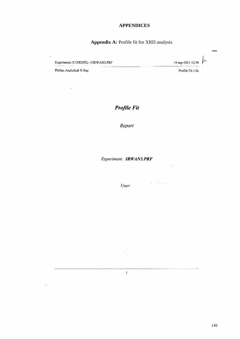
149
APPENDICES
Appendix A: Profile fit for XRD analysis

150
151

152

153

154
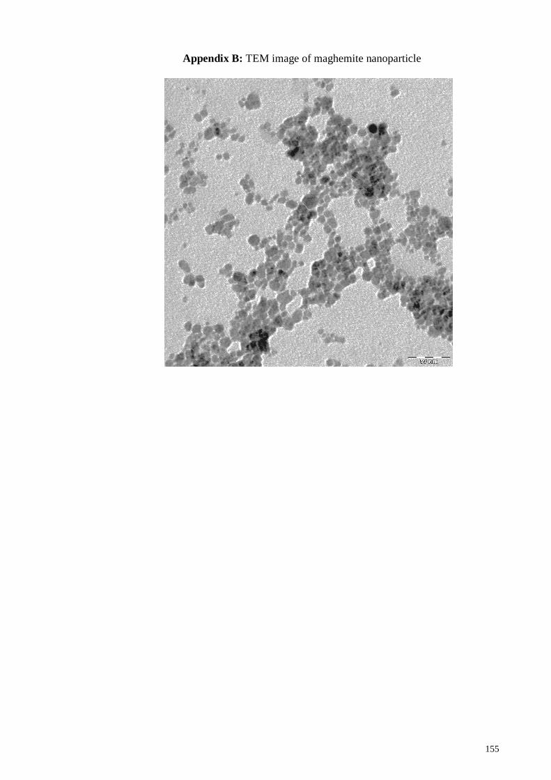
155
Appendix B: TEM image of maghemite nanoparticle

156
Appendix C: TGA thermogram of maghemite nanoparticle
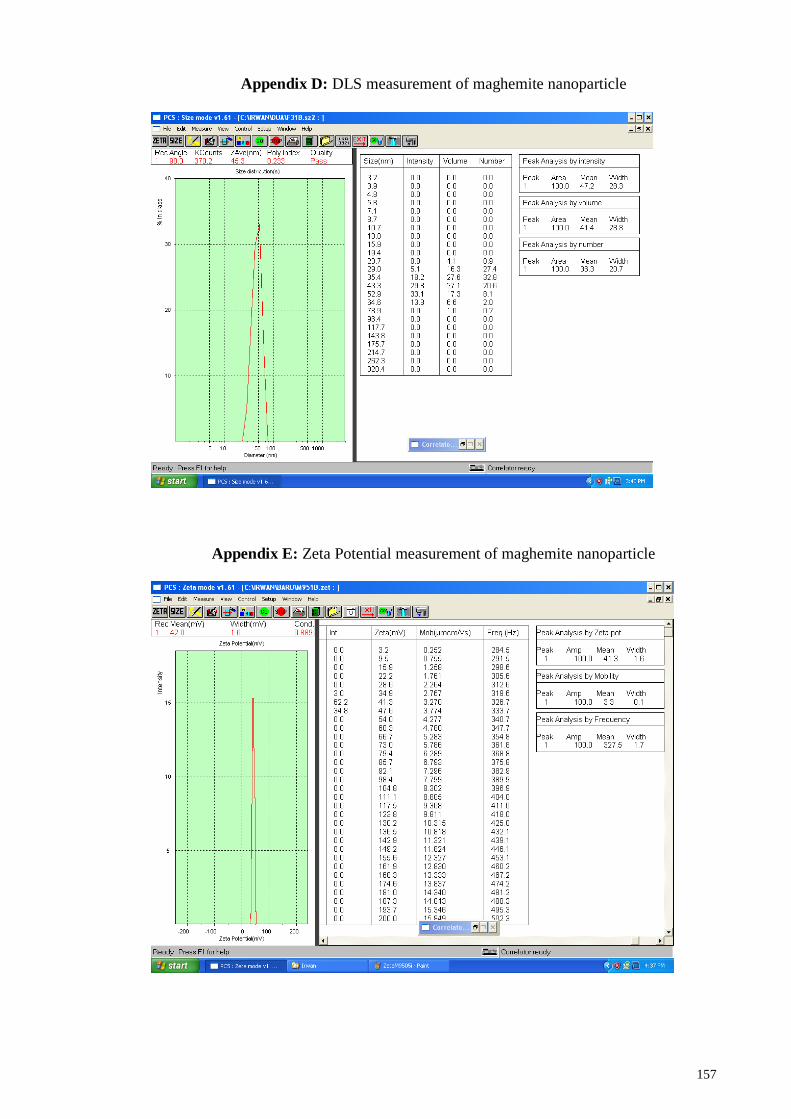
157
Appendix D: DLS measurement of maghemite nanoparticle
Appendix E: Zeta Potential measurement of maghemite nanoparticle
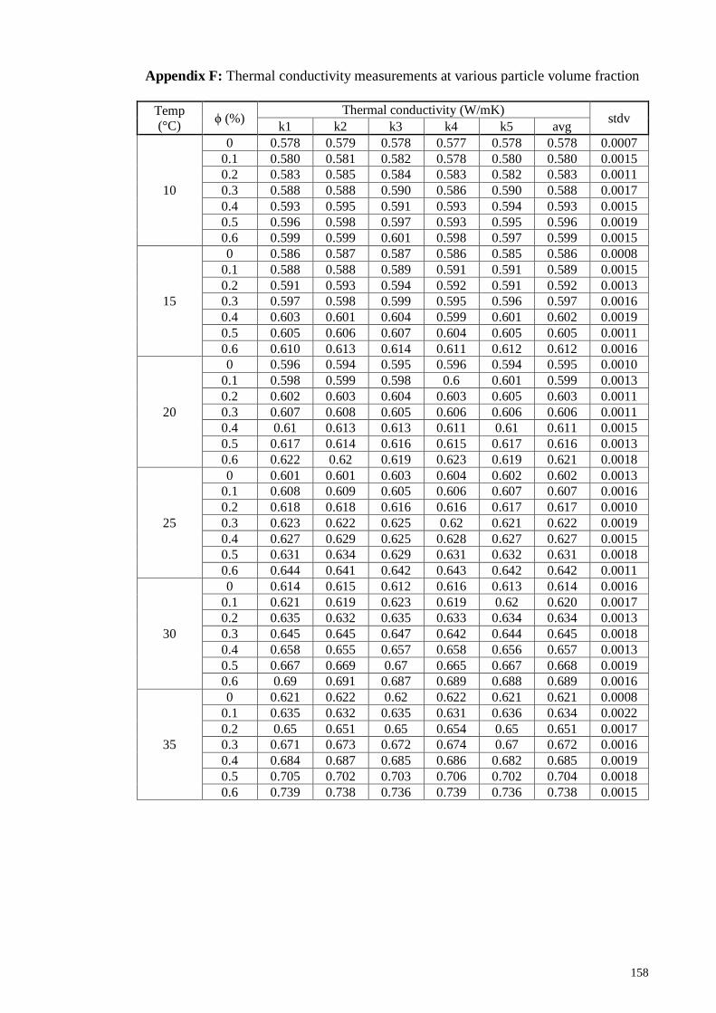
158
Appendix F: Thermal conductivity measurements at various particle volume fraction
Temp
(°C) ϕ (%)
Thermal conductivity (W/mK) stdv
k1 k2 k3 k4 k5 avg
10
0 0.578 0.579 0.578 0.577 0.578 0.578 0.0007
0.1 0.580 0.581 0.582 0.578 0.580 0.580 0.0015
0.2 0.583 0.585 0.584 0.583 0.582 0.583 0.0011
0.3 0.588 0.588 0.590 0.586 0.590 0.588 0.0017
0.4 0.593 0.595 0.591 0.593 0.594 0.593 0.0015
0.5 0.596 0.598 0.597 0.593 0.595 0.596 0.0019
0.6 0.599 0.599 0.601 0.598 0.597 0.599 0.0015
15
0 0.586 0.587 0.587 0.586 0.585 0.586 0.0008
0.1 0.588 0.588 0.589 0.591 0.591 0.589 0.0015
0.2 0.591 0.593 0.594 0.592 0.591 0.592 0.0013
0.3 0.597 0.598 0.599 0.595 0.596 0.597 0.0016
0.4 0.603 0.601 0.604 0.599 0.601 0.602 0.0019
0.5 0.605 0.606 0.607 0.604 0.605 0.605 0.0011
0.6 0.610 0.613 0.614 0.611 0.612 0.612 0.0016
20
0 0.596 0.594 0.595 0.596 0.594 0.595 0.0010
0.1 0.598 0.599 0.598 0.6 0.601 0.599 0.0013
0.2 0.602 0.603 0.604 0.603 0.605 0.603 0.0011
0.3 0.607 0.608 0.605 0.606 0.606 0.606 0.0011
0.4 0.61 0.613 0.613 0.611 0.61 0.611 0.0015
0.5 0.617 0.614 0.616 0.615 0.617 0.616 0.0013
0.6 0.622 0.62 0.619 0.623 0.619 0.621 0.0018
25
0 0.601 0.601 0.603 0.604 0.602 0.602 0.0013
0.1 0.608 0.609 0.605 0.606 0.607 0.607 0.0016
0.2 0.618 0.618 0.616 0.616 0.617 0.617 0.0010
0.3 0.623 0.622 0.625 0.62 0.621 0.622 0.0019
0.4 0.627 0.629 0.625 0.628 0.627 0.627 0.0015
0.5 0.631 0.634 0.629 0.631 0.632 0.631 0.0018
0.6 0.644 0.641 0.642 0.643 0.642 0.642 0.0011
30
0 0.614 0.615 0.612 0.616 0.613 0.614 0.0016
0.1 0.621 0.619 0.623 0.619 0.62 0.620 0.0017
0.2 0.635 0.632 0.635 0.633 0.634 0.634 0.0013
0.3 0.645 0.645 0.647 0.642 0.644 0.645 0.0018
0.4 0.658 0.655 0.657 0.658 0.656 0.657 0.0013
0.5 0.667 0.669 0.67 0.665 0.667 0.668 0.0019
0.6 0.69 0.691 0.687 0.689 0.688 0.689 0.0016
35
0 0.621 0.622 0.62 0.622 0.621 0.621 0.0008
0.1 0.635 0.632 0.635 0.631 0.636 0.634 0.0022
0.2 0.65 0.651 0.65 0.654 0.65 0.651 0.0017
0.3 0.671 0.673 0.672 0.674 0.67 0.672 0.0016
0.4 0.684 0.687 0.685 0.686 0.682 0.685 0.0019
0.5 0.705 0.702 0.703 0.706 0.702 0.704 0.0018
0.6 0.739 0.738 0.736 0.739 0.736 0.738 0.0015

159
Appendix G: Thermal conductivity measurements at various temperature
ϕ (%) T (°C) Thermal conductivity (W/mK)
stdv k1 k2 k3 k4 k5 avg
0
10 0.578 0.579 0.578 0.577 0.578 0.578 0.0007
15 0.586 0.587 0.587 0.586 0.585 0.586 0.0008
20 0.596 0.594 0.595 0.596 0.594 0.595 0.0010
25 0.601 0.601 0.603 0.604 0.602 0.602 0.0013
30 0.614 0.615 0.612 0.616 0.613 0.614 0.0016
35 0.621 0.622 0.62 0.622 0.621 0.621 0.0008
0.1
10 0.580 0.581 0.582 0.578 0.580 0.580 0.0015
15 0.588 0.588 0.589 0.591 0.591 0.589 0.0015
20 0.598 0.599 0.598 0.6 0.601 0.599 0.0013
25 0.608 0.609 0.605 0.606 0.607 0.607 0.0016
30 0.621 0.619 0.623 0.619 0.62 0.620 0.0017
35 0.635 0.632 0.635 0.631 0.636 0.634 0.0022
0.2
10 0.583 0.585 0.584 0.583 0.582 0.583 0.0011
15 0.591 0.593 0.594 0.592 0.591 0.592 0.0013
20 0.607 0.608 0.605 0.606 0.606 0.6064 0.0011
25 0.618 0.618 0.616 0.616 0.617 0.617 0.0010
30 0.635 0.632 0.635 0.633 0.634 0.634 0.0013
35 0.65 0.651 0.65 0.654 0.65 0.651 0.0017
0.3
10 0.588 0.588 0.590 0.586 0.590 0.588 0.0017
15 0.597 0.598 0.599 0.595 0.596 0.597 0.0016
20 0.622 0.62 0.619 0.623 0.619 0.621 0.0018
25 0.623 0.622 0.625 0.62 0.621 0.622 0.0019
30 0.645 0.645 0.647 0.642 0.644 0.645 0.0018
35 0.671 0.673 0.672 0.674 0.67 0.672 0.0016
0.4
10 0.593 0.595 0.591 0.593 0.594 0.593 0.0015
15 0.603 0.601 0.604 0.599 0.601 0.602 0.0019
20 0.61 0.613 0.613 0.611 0.61 0.611 0.0015
25 0.627 0.629 0.625 0.628 0.627 0.627 0.0015
30 0.658 0.655 0.657 0.658 0.656 0.657 0.0013
35 0.684 0.687 0.685 0.686 0.682 0.685 0.0019
0.5
10 0.596 0.598 0.597 0.593 0.595 0.596 0.0019
15 0.605 0.606 0.607 0.604 0.605 0.605 0.0011
20 0.617 0.614 0.616 0.615 0.617 0.616 0.0013
25 0.631 0.634 0.629 0.631 0.632 0.631 0.0018
30 0.667 0.669 0.67 0.665 0.667 0.668 0.0019
35 0.705 0.702 0.703 0.706 0.702 0.704 0.0018
0.6
10 0.599 0.599 0.601 0.598 0.597 0.599 0.0015
15 0.610 0.613 0.614 0.611 0.612 0.612 0.0016
20 0.622 0.62 0.619 0.623 0.619 0.621 0.0018
25 0.644 0.641 0.642 0.643 0.642 0.642 0.0011
30 0.69 0.691 0.687 0.689 0.688 0.689 0.0016
35 0.739 0.738 0.736 0.739 0.736 0.738 0.0015
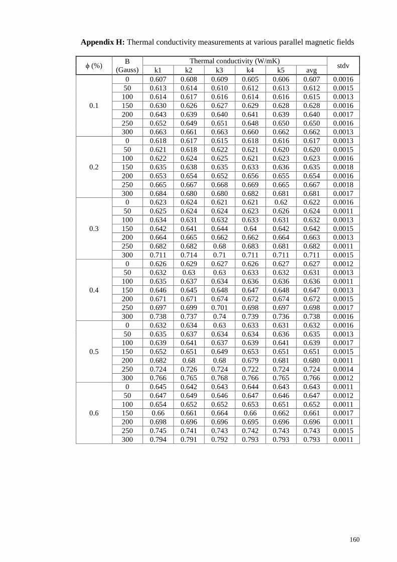
160
Appendix H: Thermal conductivity measurements at various parallel magnetic fields
ϕ (%) B
(Gauss)
Thermal conductivity (W/mK) stdv
k1 k2 k3 k4 k5 avg
0.1
0 0.607 0.608 0.609 0.605 0.606 0.607 0.0016
50 0.613 0.614 0.610 0.612 0.613 0.612 0.0015
100 0.614 0.617 0.616 0.614 0.616 0.615 0.0013
150 0.630 0.626 0.627 0.629 0.628 0.628 0.0016
200 0.643 0.639 0.640 0.641 0.639 0.640 0.0017
250 0.652 0.649 0.651 0.648 0.650 0.650 0.0016
300 0.663 0.661 0.663 0.660 0.662 0.662 0.0013
0.2
0 0.618 0.617 0.615 0.618 0.616 0.617 0.0013
50 0.621 0.618 0.622 0.621 0.620 0.620 0.0015
100 0.622 0.624 0.625 0.621 0.623 0.623 0.0016
150 0.635 0.638 0.635 0.633 0.636 0.635 0.0018
200 0.653 0.654 0.652 0.656 0.655 0.654 0.0016
250 0.665 0.667 0.668 0.669 0.665 0.667 0.0018
300 0.684 0.680 0.680 0.682 0.681 0.681 0.0017
0.3
0 0.623 0.624 0.621 0.621 0.62 0.622 0.0016
50 0.625 0.624 0.624 0.623 0.626 0.624 0.0011
100 0.634 0.631 0.632 0.633 0.631 0.632 0.0013
150 0.642 0.641 0.644 0.64 0.642 0.642 0.0015
200 0.664 0.665 0.662 0.662 0.664 0.663 0.0013
250 0.682 0.682 0.68 0.683 0.681 0.682 0.0011
300 0.711 0.714 0.71 0.711 0.711 0.711 0.0015
0.4
0 0.626 0.629 0.627 0.626 0.627 0.627 0.0012
50 0.632 0.63 0.63 0.633 0.632 0.631 0.0013
100 0.635 0.637 0.634 0.636 0.636 0.636 0.0011
150 0.646 0.645 0.648 0.647 0.648 0.647 0.0013
200 0.671 0.671 0.674 0.672 0.674 0.672 0.0015
250 0.697 0.699 0.701 0.698 0.697 0.698 0.0017
300 0.738 0.737 0.74 0.739 0.736 0.738 0.0016
0.5
0 0.632 0.634 0.63 0.633 0.631 0.632 0.0016
50 0.635 0.637 0.634 0.634 0.636 0.635 0.0013
100 0.639 0.641 0.637 0.639 0.641 0.639 0.0017
150 0.652 0.651 0.649 0.653 0.651 0.651 0.0015
200 0.682 0.68 0.68 0.679 0.681 0.680 0.0011
250 0.724 0.726 0.724 0.722 0.724 0.724 0.0014
300 0.766 0.765 0.768 0.766 0.765 0.766 0.0012
0.6
0 0.645 0.642 0.643 0.644 0.643 0.643 0.0011
50 0.647 0.649 0.646 0.647 0.646 0.647 0.0012
100 0.654 0.652 0.652 0.653 0.651 0.652 0.0011
150 0.66 0.661 0.664 0.66 0.662 0.661 0.0017
200 0.698 0.696 0.696 0.695 0.696 0.696 0.0011
250 0.745 0.741 0.743 0.742 0.743 0.743 0.0015
300 0.794 0.791 0.792 0.793 0.793 0.793 0.0011

161
Appendix I: Thermal conductivity measurements at various
perpendicular magnetic fields
ϕ (%) B
(Gauss)
Thermal conductivity (W/mK) stdv
k1 k2 k3 k4 k5 avg
0.1
0 0.608 0.604 0.608 0.607 0.607 0.607 0.0016
50 0.609 0.606 0.609 0.608 0.609 0.608 0.0013
100 0.609 0.607 0.609 0.610 0.608 0.609 0.0011
150 0.609 0.611 0.610 0.612 0.612 0.611 0.0013
200 0.612 0.613 0.611 0.611 0.613 0.612 0.0010
250 0.614 0.615 0.613 0.614 0.612 0.614 0.0011
300 0.614 0.614 0.616 0.612 0.614 0.614 0.0014
0.2
0 0.616 0.618 0.616 0.619 0.617 0.617 0.0013
50 0.617 0.615 0.618 0.619 0.618 0.617 0.0015
100 0.618 0.617 0.618 0.619 0.620 0.618 0.0011
150 0.621 0.623 0.624 0.621 0.621 0.622 0.0014
200 0.625 0.623 0.624 0.625 0.622 0.624 0.0013
250 0.625 0.626 0.625 0.624 0.627 0.625 0.0011
300 0.627 0.628 0.629 0.627 0.626 0.627 0.0011
0.3
0 0.621 0.623 0.624 0.621 0.622 0.622 0.0013
50 0.622 0.62 0.624 0.624 0.622 0.622 0.0017
100 0.625 0.625 0.626 0.623 0.627 0.625 0.0015
150 0.626 0.628 0.629 0.626 0.628 0.627 0.0013
200 0.629 0.631 0.632 0.629 0.63 0.630 0.0013
250 0.632 0.634 0.631 0.633 0.632 0.632 0.0011
300 0.632 0.633 0.634 0.632 0.635 0.633 0.0013
0.4
0 0.627 0.628 0.626 0.629 0.625 0.627 0.0016
50 0.629 0.627 0.631 0.63 0.629 0.629 0.0015
100 0.631 0.63 0.634 0.633 0.633 0.632 0.0016
150 0.636 0.636 0.634 0.633 0.635 0.635 0.0013
200 0.636 0.637 0.639 0.636 0.639 0.637 0.0015
250 0.64 0.643 0.639 0.643 0.641 0.641 0.0018
300 0.643 0.643 0.645 0.641 0.643 0.643 0.0014
0.5
0 0.63 0.632 0.633 0.629 0.63 0.631 0.0016
50 0.633 0.634 0.633 0.631 0.635 0.633 0.0015
100 0.637 0.635 0.637 0.634 0.636 0.636 0.0013
150 0.64 0.639 0.641 0.638 0.639 0.639 0.0011
200 0.64 0.641 0.643 0.64 0.643 0.641 0.0015
250 0.646 0.645 0.644 0.643 0.647 0.645 0.0016
300 0.649 0.652 0.65 0.651 0.65 0.650 0.0011
0.6
0 0.643 0.644 0.642 0.645 0.641 0.643 0.0016
50 0.643 0.645 0.643 0.646 0.645 0.644 0.0013
100 0.645 0.646 0.644 0.647 0.645 0.645 0.0011
150 0.649 0.648 0.646 0.649 0.647 0.648 0.0013
200 0.65 0.652 0.65 0.653 0.65 0.651 0.0014
250 0.655 0.653 0.655 0.652 0.656 0.654 0.0016
300 0.657 0.655 0.656 0.655 0.658 0.656 0.0013

162
Appendix J: Kinematic viscosity measurements at various particle volume fraction
ϕ t (sec) µ (cst) µavrg (cst) stdv
0
335.32 1.306
1.307 0.0019
335.65 1.307
335.69 1.308
336.46 1.311
335.17 1.305
0.1
337.65 1.315
1.316 0.0016
338.65 1.319
337.86 1.316
337.67 1.315
337.98 1.316
0.2
338.54 1.319
1.319 0.0018
338.64 1.319
338.67 1.319
338.3 1.318
339.52 1.322
0.3
339.28 1.321
1.323 0.0017
339.43 1.322
340.32 1.326
339.67 1.323
340.12 1.325
0.4
340.89 1.328
1.328 0.0019
340.41 1.326
340.62 1.327
341.65 1.331
340.57 1.327
0.5
341.67 1.331
1.332 0.0019
342.61 1.334
341.76 1.331
341.85 1.332
342.63 1.335
0.6
343.54 1.338
1.337 0.0012
342.98 1.336
342.78 1.335
343.46 1.338
343.23 1.337

163
Appendix K: Kinematic viscosity measurements at various temperature
T (oC) t (sec) µ (cst) µavrg (cst) stdv
10
335.32 1.306
1.307 0.0019
335.65 1.307
335.69 1.308
336.46 1.311
335.17 1.305
15
293.86 1.144
1.144 0.0015
293.76 1.144
293.15 1.142
294.22 1.146
293.55 1.143
20
256.78 0.999
0.997 0.0023
255.46 0.994
256.43 0.998
255.72 0.995
256.64 0.999
25
229.1 0.891
0.889 0.0019
228.54 0.889
227.89 0.887
227.98 0.887
228.64 0.890
30
205.23 0.798
0.799 0.0011
205.54 0.799
205.17 0.798
205.86 0.801
205.43 0.799
35
187.78 0.730
0.732 0.0012
188.42 0.733
188.19 0.732
188.62 0.733
188.36 0.732

164
Appendix L: Kinematic viscosity measurements at various parallel magnetic fields
Magnetic fields
(Gauss) t (sec) µ (cst) µavrg
(cst) stdv
0
231.67 0.901
0.901 0.0014
231.54 0.901
231.12 0.899
231.76 0.902
232.14 0.903
50
232.86 0.906
0.905 0.0017
232.63 0.905
231.72 0.902
232.57 0.905
232.71 0.905
100
235.54 0.916
0.914 0.0020
235.13 0.915
234.72 0.913
234.81 0.914
234.17 0.911
150
238.56 0.928
0.927 0.0016
238.91 0.930
238.15 0.927
237.84 0.925
238.28 0.927
200
241.15 0.938
0.941 0.0015
242.18 0.942
241.65 0.940
241.86 0.941
241.89 0.941
250
244.76 0.952
0.952 0.0016
244.13 0.950
245.25 0.954
244.61 0.952
244.82 0.953
300
248.73 0.968
0.969 0.0012
249.16 0.969
249.26 0.970
248.67 0.968
249.32 0.970
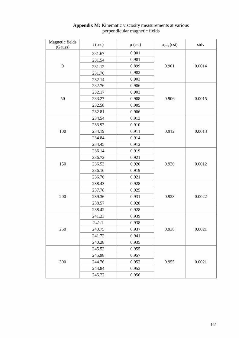
165
Appendix M: Kinematic viscosity measurements at various
perpendicular magnetic fields
Magnetic fields
(Gauss) t (sec) µ (cst) µavrg
(cst) stdv
0
231.67 0.901
0.901 0.0014
231.54 0.901
231.12 0.899
231.76 0.902
232.14 0.903
50
232.76 0.906
0.906 0.0015
232.17 0.903
233.27 0.908
232.58 0.905
232.81 0.906
100
234.54 0.913
0.912 0.0013
233.97 0.910
234.19 0.911
234.84 0.914
234.45 0.912
150
236.14 0.919
0.920 0.0012
236.72 0.921
236.53 0.920
236.16 0.919
236.76 0.921
200
238.43 0.928
0.928 0.0022
237.78 0.925
239.36 0.931
238.57 0.928
238.42 0.928
250
241.23 0.939
0.938 0.0021
241.1 0.938
240.75 0.937
241.72 0.941
240.28 0.935
300
245.52 0.955
0.955 0.0021
245.98 0.957
244.76 0.952
244.84 0.953
245.72 0.956

166
Appendix N: Electrical conductivity measurements at various particle volume fraction
Temp
(°C) ϕ (%)
Electrical conductivity (mS/cm) stdv
σ1 σ2 σ3 σ4 σ5 σavg
10
0.1 0.868 0.867 0.866 0.868 0.869 0.868 0.0011
0.2 1.460 1.462 1.462 1.460 1.463 1.461 0.0013
0.3 2.164 2.164 2.166 2.163 2.167 2.165 0.0016
0.4 2.753 2.754 2.753 2.752 2.756 2.754 0.0015
0.5 3.376 3.378 3.379 3.379 3.377 3.378 0.0013
0.6 4.046 4.044 4.047 4.045 4.046 4.046 0.0011
15
0.1 0.946 0.946 0.948 0.947 0.948 0.947 0.0010
0.2 1.644 1.645 1.647 1.643 1.647 1.645 0.0018
0.3 2.560 2.562 2.563 2.561 2.560 2.561 0.0013
0.4 3.318 3.316 3.318 3.319 3.317 3.318 0.0011
0.5 4.203 4.204 4.202 4.205 4.207 4.204 0.0019
0.6 5.192 5.196 5.193 5.194 5.195 5.194 0.0016
20
0.1 0.991 0.992 0.989 0.988 0.99 0.990 0.0016
0.2 1.813 1.815 1.813 1.812 1.816 1.814 0.0016
0.3 2.82 2.818 2.817 2.819 2.82 2.819 0.0013
0.4 3.689 3.689 3.687 3.689 3.686 3.688 0.0014
0.5 4.642 4.643 4.642 4.644 4.644 4.643 0.0010
0.6 5.672 5.674 5.672 5.675 5.673 5.673 0.0013
25
0.1 1.011 1.008 1.01 1.011 1.011 1.010 0.0013
0.2 1.986 1.987 1.986 1.984 1.987 1.986 0.0012
0.3 3.111 3.109 3.107 3.11 3.108 3.109 0.0016
0.4 4.107 4.106 4.104 4.108 4.109 4.107 0.0019
0.5 4.99 4.991 4.989 4.992 4.993 4.991 0.0016
0.6 6.618 6.616 6.618 6.619 6.614 6.617 0.0020
30
0.1 1.05 1.049 1.053 1.052 1.051 1.051 0.0016
0.2 2.168 2.169 2.168 2.167 2.166 2.168 0.0011
0.3 3.375 3.376 3.374 3.377 3.373 3.375 0.0016
0.4 4.367 4.368 4.368 4.367 4.366 4.367 0.0008
0.5 5.455 5.456 5.457 5.458 5.455 5.456 0.0013
0.6 6.68 6.682 6.682 6.681 6.68 6.681 0.0010
35
0.1 1.101 1.101 1.101 1.103 1.103 1.102 0.0011
0.2 2.376 2.376 2.377 2.375 2.376 2.376 0.0007
0.3 3.643 3.644 3.642 3.645 3.644 3.644 0.0011
0.4 4.744 4.745 4.745 4.746 4.745 4.745 0.0007
0.5 5.998 5.998 5.998 5.998 5.996 5.998 0.0009
0.6 7.347 7.348 7.345 7.348 7.35 7.348 0.0018

167
Appendix O: Electrical conductivity measurements at various temperature
ϕ (%) T (°C) Electrical conductivity (mS/cm)
stdv σ1 σ2 σ3 σ4 σ5 σavg
0.1
10 0.868 0.867 0.866 0.868 0.869 0.868 0.0011
15 0.946 0.946 0.948 0.947 0.948 0.947 0.0010
20 0.991 0.992 0.989 0.988 0.99 0.990 0.0016
25 1.011 1.008 1.01 1.011 1.011 1.010 0.0013
30 1.05 1.049 1.053 1.052 1.051 1.051 0.0016
35 1.101 1.101 1.101 1.103 1.103 1.102 0.0011
0.2
10 1.460 1.462 1.462 1.460 1.463 1.461 0.0013
15 1.644 1.645 1.647 1.643 1.647 1.645 0.0018
20 1.813 1.815 1.813 1.812 1.816 1.8138 0.0016
25 1.986 1.987 1.986 1.984 1.987 1.986 0.0012
30 2.168 2.169 2.168 2.167 2.166 2.168 0.0011
35 2.376 2.376 2.377 2.375 2.376 2.376 0.0007
0.3
10 2.164 2.164 2.166 2.163 2.167 2.165 0.0016
15 2.560 2.562 2.563 2.561 2.560 2.561 0.0013
20 2.82 2.818 2.817 2.819 2.82 2.819 0.0013
25 3.111 3.109 3.107 3.11 3.108 3.109 0.0016
30 3.375 3.376 3.374 3.377 3.373 3.375 0.0016
35 3.643 3.644 3.642 3.645 3.644 3.644 0.0011
0.4
10 2.753 2.754 2.753 2.752 2.756 2.754 0.0015
15 3.318 3.316 3.318 3.319 3.317 3.318 0.0011
20 3.689 3.689 3.687 3.689 3.686 3.688 0.0014
25 4.107 4.106 4.104 4.108 4.109 4.107 0.0019
30 4.367 4.368 4.368 4.367 4.366 4.367 0.0008
35 4.744 4.745 4.745 4.746 4.745 4.745 0.0007
0.5
10 3.376 3.378 3.379 3.379 3.377 3.378 0.0013
15 4.203 4.204 4.202 4.205 4.207 4.204 0.0019
20 4.642 4.643 4.642 4.644 4.644 4.643 0.0010
25 4.99 4.991 4.989 4.992 4.993 4.991 0.0016
30 5.455 5.456 5.457 5.458 5.455 5.456 0.0013
35 5.998 5.998 5.998 5.998 5.996 5.998 0.0009
0.6
10 4.046 4.044 4.047 4.045 4.046 4.046 0.0011
15 5.192 5.196 5.193 5.194 5.195 5.194 0.0016
20 5.672 5.674 5.672 5.675 5.673 5.673 0.0013
25 6.618 6.616 6.618 6.619 6.614 6.617 0.0020
30 6.68 6.682 6.682 6.681 6.68 6.681 0.0010
35 7.347 7.348 7.345 7.348 7.35 7.348 0.0018
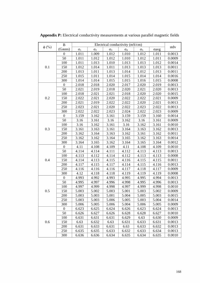
168
Appendix P: Electrical conductivity measurements at various parallel magnetic fields
ϕ (%) B
(Gauss)
Electrical conductivity (mS/cm) stdv
σ1 σ2 σ3 σ4 σ5 σavg
0.1
0 1.011 1.009 1.012 1.010 1.012 1.011 0.0013
50 1.011 1.012 1.012 1.010 1.012 1.011 0.0009
100 1.011 1.013 1.010 1.013 1.013 1.012 0.0014
150 1.012 1.014 1.011 1.013 1.013 1.013 0.0011
200 1.013 1.011 1.013 1.014 1.012 1.013 0.0011
250 1.015 1.011 1.014 1.015 1.014 1.014 0.0016
300 1.014 1.014 1.015 1.015 1.016 1.015 0.0008
0.2
0 2.018 2.018 2.020 2.017 2.020 2.019 0.0013
50 2.021 2.019 2.018 2.020 2.021 2.020 0.0013
100 2.018 2.021 2.021 2.018 2.020 2.020 0.0015
150 2.022 2.021 2.020 2.022 2.022 2.021 0.0009
200 2.021 2.019 2.022 2.022 2.020 2.021 0.0013
250 2.023 2.021 2.020 2.022 2.023 2.022 0.0013
300 2.022 2.022 2.023 2.024 2.022 2.023 0.0009
0.3
0 3.159 3.162 3.161 3.159 3.159 3.160 0.0014
50 3.16 3.161 3.16 3.162 3.16 3.161 0.0009
100 3.16 3.162 3.161 3.16 3.162 3.161 0.0010
150 3.161 3.163 3.161 3.164 3.163 3.162 0.0013
200 3.162 3.164 3.163 3.162 3.161 3.162 0.0011
250 3.162 3.162 3.164 3.165 3.162 3.163 0.0014
300 3.164 3.165 3.162 3.164 3.165 3.164 0.0012
0.4
0 4.11 4.108 4.109 4.11 4.108 4.109 0.0010
50 4.114 4.114 4.111 4.112 4.113 4.113 0.0013
100 4.113 4.112 4.114 4.112 4.113 4.113 0.0008
150 4.114 4.113 4.115 4.116 4.115 4.115 0.0011
200 4.117 4.115 4.117 4.114 4.115 4.116 0.0013
250 4.116 4.116 4.116 4.117 4.118 4.117 0.0009
300 4.12 4.118 4.118 4.119 4.119 4.119 0.0008
0.5
0 4.993 4.992 4.993 4.995 4.995 4.994 0.0013
50 4.995 4.997 4.996 4.998 4.995 4.996 0.0013
100 4.997 4.999 4.998 4.997 4.999 4.998 0.0010
150 5.003 5.002 5.003 5.001 5.003 5.002 0.0009
200 5.003 5.003 5.001 5.004 5.005 5.003 0.0015
250 5.003 5.003 5.006 5.005 5.003 5.004 0.0014
300 5.006 5.005 5.006 5.004 5.006 5.005 0.0009
0.6
0 6.623 6.625 6.624 6.626 6.623 6.624 0.0013
50 6.626 6.627 6.626 6.628 6.628 6.627 0.0010
100 6.631 6.631 6.631 6.629 6.63 6.630 0.0009
150 6.63 6.632 6.63 6.631 6.633 6.631 0.0013
200 6.631 6.633 6.631 6.63 6.633 6.632 0.0013
250 6.635 6.635 6.633 6.632 6.633 6.634 0.0013
300 6.636 6.636 6.634 6.635 6.634 6.635 0.0010

169
Appendix Q: Electrical conductivity measurements at various
perpendicular magnetic fields
φ (%) B
(Gauss)
Electrical conductivity (mS/cm) stdv
σ1 σ2 σ3 σ4 σ5 σavg
0.1
0 1.011 1.013 1.014 1.012 1.013 1.013 0.0011
50 1.015 1.017 1.015 1.016 1.017 1.016 0.0010
100 1.019 1.016 1.019 1.017 1.018 1.018 0.0013
150 1.019 1.020 1.019 1.021 1.021 1.020 0.0010
200 1.020 1.022 1.023 1.021 1.021 1.021 0.0011
250 1.021 1.022 1.023 1.024 1.021 1.022 0.0013
300 1.022 1.023 1.024 1.023 1.021 1.023 0.0011
0.2
0 2.020 2.019 2.019 2.018 2.018 2.019 0.0008
50 2.023 2.022 2.023 2.021 2.023 2.022 0.0009
100 2.022 2.023 2.024 2.024 2.022 2.023 0.0010
150 2.024 2.025 2.024 2.025 2.023 2.024 0.0008
200 2.024 2.024 2.025 2.026 2.026 2.025 0.0010
250 2.028 2.026 2.027 2.028 2.028 2.027 0.0009
300 2.027 2.027 2.028 2.029 2.027 2.028 0.0009
0.3
0 3.131 3.13 3.132 3.13 3.129 3.130 0.0011
50 3.134 3.133 3.132 3.134 3.132 3.133 0.0010
100 3.136 3.133 3.136 3.135 3.136 3.135 0.0013
150 3.136 3.137 3.135 3.137 3.139 3.137 0.0015
200 3.14 3.139 3.138 3.14 3.137 3.139 0.0013
250 3.138 3.139 3.14 3.138 3.14 3.139 0.0010
300 3.14 3.141 3.14 3.142 3.139 3.140 0.0011
0.4
0 4.117 4.118 4.119 4.118 4.12 4.118 0.0011
50 4.119 4.121 4.121 4.119 4.12 4.120 0.0010
100 4.121 4.121 4.122 4.12 4.122 4.121 0.0008
150 4.122 4.123 4.122 4.124 4.124 4.123 0.0010
200 4.123 4.123 4.124 4.121 4.125 4.123 0.0015
250 4.125 4.123 4.125 4.125 4.124 4.124 0.0009
300 4.124 4.125 4.126 4.126 4.124 4.125 0.0010
0.5
0 5.008 5.006 5.007 5.009 5.008 5.008 0.0011
50 5.01 5.011 5.012 5.012 5.01 5.011 0.0010
100 5.011 5.012 5.013 5.014 5.011 5.012 0.0013
150 5.013 5.014 5.013 5.015 5.015 5.014 0.0010
200 5.015 5.014 5.016 5.016 5.015 5.015 0.0008
250 5.014 5.016 5.015 5.017 5.016 5.016 0.0011
300 5.018 5.018 5.017 5.016 5.017 5.017 0.0008
0.6
0 6.627 6.627 6.629 6.627 6.628 6.628 0.0009
50 6.630 6.631 6.630 6.632 6.629 6.630 0.0011
100 6.63 6.629 6.632 6.632 6.63 6.631 0.0013
150 6.633 6.633 6.634 6.632 6.635 6.633 0.0011
200 6.632 6.634 6.632 6.635 6.634 6.633 0.0013
250 6.633 6.635 6.634 6.633 6.634 6.634 0.0008
300 6.634 6.635 6.636 6.634 6.634 6.635 0.0009