Sub-microsecond temperature measurement in … be submitted to Applied Optics 1 Sub-microsecond...

To be submitted to Applied Optics

1

Sub-microsecond temperature measurement

in liquid water using laser-induced thermal acoustics

David W. Alderfer, G. C. Herring, Paul M. Danehy

NASA Langley Research Center

18 Langley Blvd, Mail stop 493, Hampton VA, 23681-2199, USA

Toshiharu Mizukaki

The 1st ReC, TRDI, JDA

2-2-1, Nakameguro, Meguro, Tokyo, 153-8630 Japan

Kazuyoshi Takayama

Shock Wave Research Center, Institute of Fluid Science,

Tohoku University, Sendai, 980-8577, Japan

Abstract: Using laser-induced thermal acoustics, we demonstrate non-intrusive and remote

sound speed and temperature measurements over the range 10 – 45 °C in liquid water. Averaged

accuracy of sound speed and temperature measurements (10 s) are 0.64 m/s and 0.45 °C

respectively. Single-shot precisions based on one standard deviation of 100 or greater samples

range from 1 m/s to 16.5 m/s and 0.3 °C to 9.5 °C for sound speed and temperature

measurements respectively. The time resolution of each single-shot measurement was 300 nsec.

©2004 Optical Society of America

OCIS codes: 300.2570, 120.6780, 120.4640, 120.0280, 120.5820, 290.5900.

https://ntrs.nasa.gov/search.jsp?R=20090014198 2018-07-03T21:45:48+00:00Z

Alderfer et al. “Sub-microsecond temperature measurement…”

2

1. Introduction

Fast non-intrusive temperature measurements are needed for numerous applications. This is

especially true for the study of shock waves. Bio-medical shock wave applications such as

Extracoporeal Shock Wave Lithotripsy (ESWL) have revealed collateral damage to healthy

tissue, in addition to the targeted cancerous tissue.1,2,3 To facilitate the understanding of the

damage mechanism and to predict the amount of damage, scientists are studying shock waves in

fluids that have acoustic properties similar to human tissue.

For relatively strong shocks with overpressures of 10-100 GPa (100-1000 katm) propagating

through liquids, the associated temperatures of ~ 5000 K generate strong thermal radiation in the

visible region and can be measured with optical pyrometry.4 For weaker shocks (~ 1 katm) used

in ESWL the situation is different, since the associated temperature jumps of ~ 10 K are not large

enough to generate appreciable visible radiative emission. The pressure histories of these weaker

shocks waves are easily studied with hydrophones1 and reveal sharp (~300 ns) pressure

increases. But, temperature measurements with similar temporal resolution are not routine, for

example, thermocouples are relatively slow (> 100 μs). Previous work5 has demonstrated ns-

temporal resolution in shock wave studies, however only under special conditions (1-

dimensional geometry with a line-of-sight diagnostic) and for parameters other than temperature.

Thus, we anticipate that future shock-wave research will benefit from the development of

additional non-intrusive, spatially resolved, and fast (< 1 μs) temperature measurement

techniques.

There are several optical temperature measurement techniques that demand consideration

for fast, spatially-precise non-intrusive temperature measurements in liquid water. Karl et al.6


3

describe two optical temperature measurement techniques that use Raman spectroscopy. One

uses a single laser beam and the other uses a laser sheet. Both techniques extract temperature

from spectroscopic information obtained from the intensity ratio at two wavelengths. Both

techniques use long integration times necessitated by the use of continuous wave (cw) lasers. By

employing a high-powered pulse laser and two intensified charge coupled device (ICCD)

cameras, this technique might have potential for single shot, spatially precise water temperature

measurements, but likely would still suffer from low signal-to-noise ratio (SNR) and, thus,

imprecise temperature/sound speed measurements. If larger laser intensities were used, the water

would most likely “break down”, forming bubbles.

Other potential temperature measurement techniques include fluorescence and Brillouin

scattering. According to Lou et al.,7 thermochromic shifts (i.e. the peak fluorescence wavelength

shifts to higher frequencies with increasing temperature) from various dyes doped into water are

useful for measuring large temperature changes. Typical shifts are on the order of 0.1 nm/°C,

making temperature measurement resolution, in water, impractical below temperature

differences less than about 10°C, according to the authors. Another fluorescence technique

described by the same authors uses the ratio of monomer-to-excimer fluorescence to determine

temperature. While this method may be precise enough to study shock waves in liquids, single-

shot measurements have not yet been demonstrated. Fry et al.8, measured the sound speed and

temperature and salinity of ocean water by measuring the Brillouin width and shift using

Brillouin LIDAR. Because of low signal levels, about 10 laser shots are integrated. In the

application of measuring rapidly moving shock waves, ranging requirements for spatial

resolution would require such short laser pulses that they would be too spectrally broad to


4

observe the Brillouin linewidth. Furthermore, these optical techniques involve time averaging

or multiple shots because of low SNR.

The laser-induced thermal acoustics (LITA) method, an optical method that produces a

relatively strong coherent signal, has been used extensively for fast, remote sound speed and

temperature measurements in gaseous flows.9-13 In liquids, Nagasaka et al.14 used a technique

very similar to our LITA setup (however, using thermal gratings instead of electrostriction

gratings), called forced Rayleigh scattering. They used this method to measure the thermal

conductivity of various samples, including water. This technique, using thermal gratings, has the

disadvantage of adding significantly more heat to the sample medium than the electrostriction

gratings version used in the present paper. Similarly, Maznev et al.15 used a laser-induced

grating technique to make quick non-contact acoustic measurements in water and on transparent

biological materials over a frequency range 30 MHz to 1 GHz to determine the dependence of

the acoustic attenuation on frequency. Measurements were made over several hundreds of laser

shots. Like those of Nagasaka et al., these measurements used absorbing laser wavelengths,

resulting in the domination of thermal gratings. However, neither of these two research groups

reported using the oscillation frequency to determine the sound speed/temperature of the host

liquid.

In this paper, we present the use of LITA with electrostrictive gratings for measuring sound

speed in liquid water, from which temperature can be inferred, with a time resolution of better

than 1 μs. Water, which makes up approximately 95% of the human body, is an obvious

candidate for preliminary investigations, and has an acoustic impedance close to living tissue.2

The thermodynamic properties of water will limit the useful temperature range of this LITA

technique to ~ 5-75 °C.


5

2. LITA Background

The LITA method involves the crossing of three laser beams. These three beams interact

with the medium to produce a fourth called the signal beam. Two input pump beams form a

grating in the medium. A third input beam, the probe, scatters from this grating, producing a

signal beam that is temporally modulated according to the properties of the medium.

The simplified idea behind LITA is that an intense stationary electromagnetic interference

pattern is produced in the medium (pure water in our experiment) during the 10-ns pump pulse.

In water, there is very little absorption of the light wave energy at 532 and 488 nm, and the

electrostriction process dominates over the thermal grating process. Water molecules, attracted

to areas of high electric field, rapidly begin moving from low- to high-field regions. The

movement of water molecules necessitates an increase in density in the regions of high electric

field and a decrease in the density in the regions of the lower electric field. A pair of induced

sound waves counter-propagate away from the interaction region, creating a dynamic density

grating, and thus dynamic index of refraction grating that modulates the scattering of the incident

probe beam according to the properties of the medium.

3. Measurement Method

In this paper, temperature is inferred from speed of sound, which is measured from the

ultrasonic modulation frequency of the LITA signal. We have used an empirical equation, the

sum of an exponential and two sine-exponential products with a LabVIEW curve-fitting

algorithm, to determine the oscillation frequency of the signal.

To determine the sound speed from the measured frequency we start with the sound speed

relationship c = Λν, where c, Λ, and ν are the sound speed, acoustic wavelength, and acoustic


6

frequency respectively. Eichler et al.16 express Λ in terms of the laser pump wavelength (λp) by

the following expression:

)2

sin(2 θλp=Λ (1)

where θ is the total pump beam crossing angle. The beat frequency for electrostriction gratings

is twice the thermalization beat frequency as discussed by Cummings et al.17 Therefore ν = f/2,

where f is the observed/measured electrostriction frequency. If we substitute Equation 1 and ν =

f/2 into c = Λν we arrive at the LITA electrostriction frequency relationship with the sound

speed:

)2

sin(4c

θλ fp= (2)

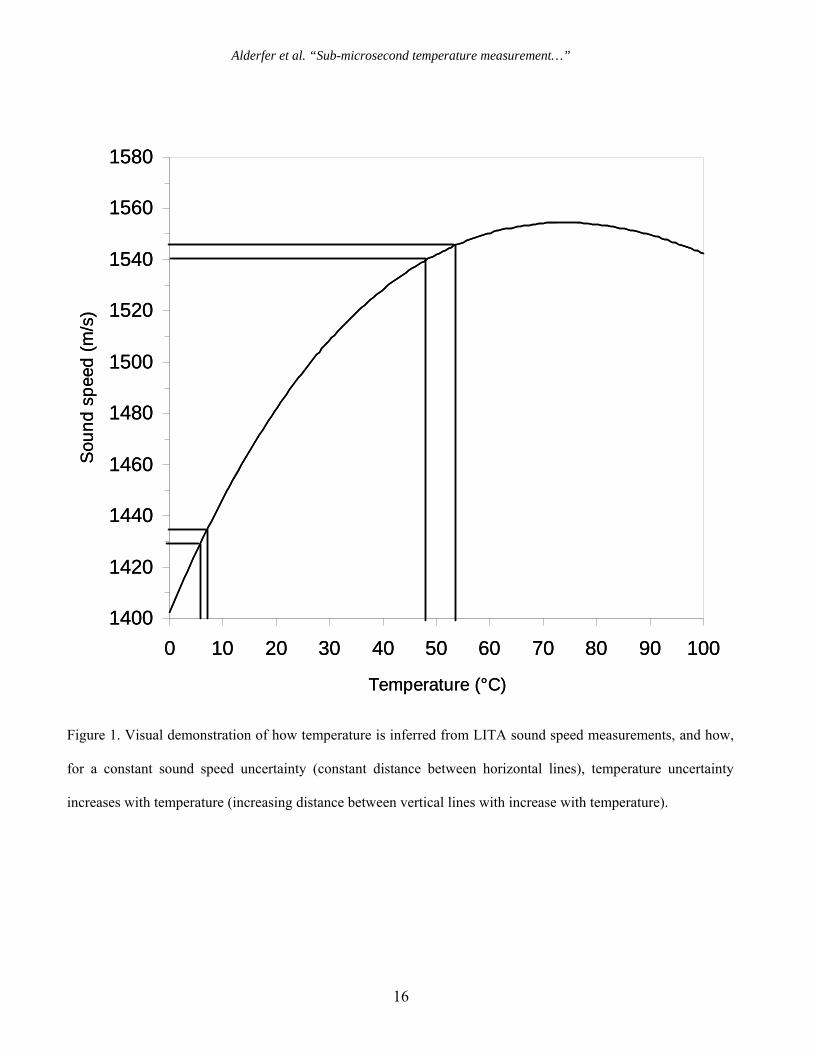
Temperature is determined from a polynomial fit of a transposed expression developed by

Chavez, Sosa, and Tsumura18 shown in Figure 1. Using a commercial spreadsheet, we plot

Chávez et al. sound speed versus temperature between the region of 10 – 75 °C with sound speed

plotted as the independent variable. We then fit a 6th order polynomial to this data. Using the 6th

order polynomial we then were able to directly relate LITA measured sound speed to

temperature. In water, the sound speed approaches 1555 m/s near 75 °C and then decreases after

that, thus the technique is double valued and very insensitive near this peak. Furthermore, this

peak sound speed value presents a problem when noise in the measurement causes the sound

speed to be measured above 1555 m/s because there is no temperature correlation above this

value. Therefore, as a simple solution, we extrapolate the range of the 6th order polynomial

above 75 °C so that sound speeds above 1555 m/s registered as temperatures above 75 °C,

although this is not physically possible. As mentioned above, the sound speed increases more

rapidly with temperature at lower temperatures and less rapidly at moderate temperatures,


7

reaching a zero rate of increase near 75 °C and decreasing thereafter. This is visually

demonstrated in Figure 1, where it is shown that there is an increase in the temperature

uncertainty (represented by the distance between the vertical lines) with increasing temperature

in the region between 10 - 75 °C, assuming constant uncertainty (distance between the horizontal

lines) in speed of sound.

Using this method requires either a very accurate measurement of the beam crossing angle

or a calibration point determined at a known temperature. We use the latter method at ambient

temperature, where the water is the most uniform in temperature and the least agitated, i.e. the

least amount of bubbles and thermal currents.

4. Experimental setup

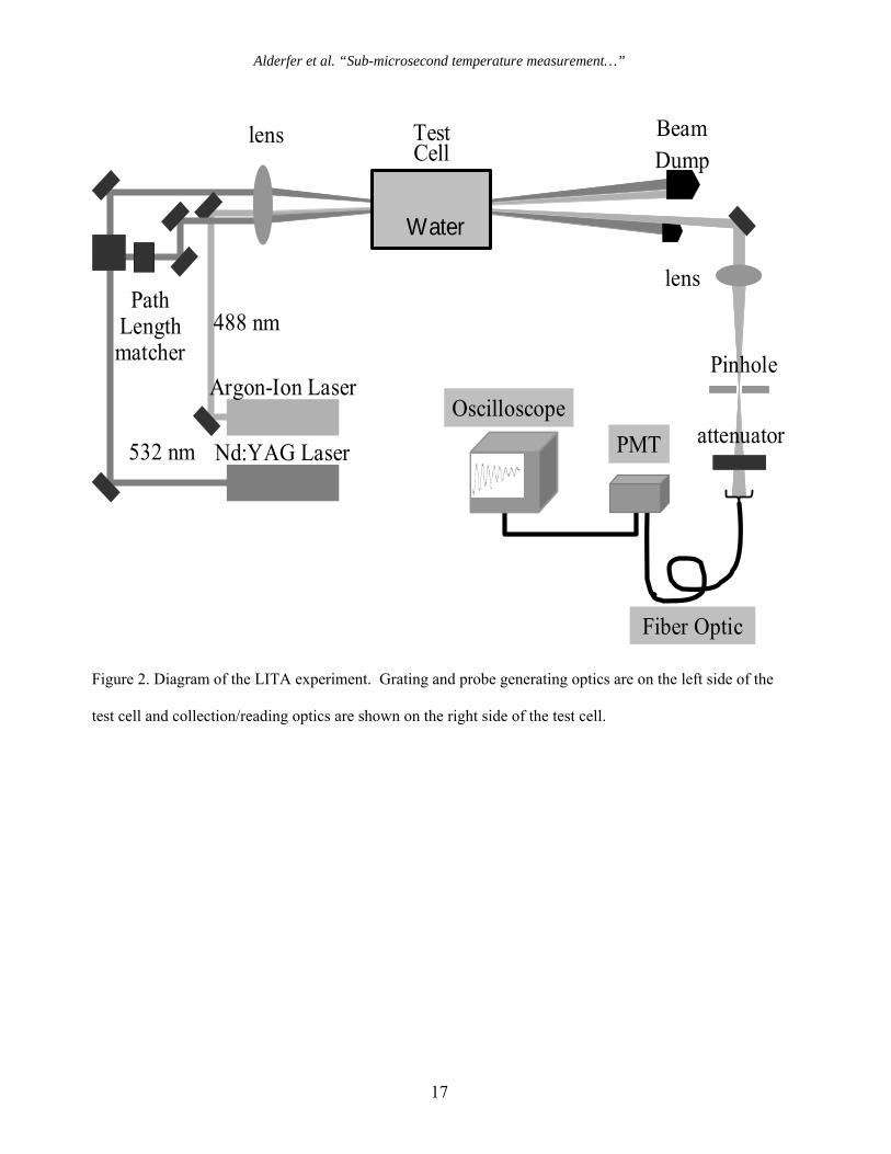
Figure 2 shows a diagram of the experiment. The setup included two lasers: a 10-ns pulsed,

frequency-doubled Nd:YAG laser operating at 532 nm and 10 Hz, and a continuous wave

Argon-ion laser operating at 488 nm. After splitting the 532 nm pump beam with a 50/50 beam

splitter, the energy of each pump beam used was about 1 mJ/pulse. The power of the 488-nm

probe beam was approximately 400 mW. The probe beam was acoustically-optically modulated,

with an approximately 10 μs pulse, to prevent scattered light from continuously entering the

photodetector.

An electrostriction grating can be formed and read out by pump and probe beams of nearly

any wavelength. In contrast, thermal gratings are formed and dominate, only, when the pump

laser wavelength matches a strong absorption in the sample. For the grating-forming pump

beams, 532 nm was chosen for two reasons. First, there is very little absorption in water at 532

nm, which is paramount when using electrostriction as the dominating grating-forming

mechanism. Secondly, 532 nm light was readily available from a 10-ns pulse Nd:YAG laser.


8

The probe wavelength was chosen as 488 nm because it also has little absorption in water and

because its wavelength separation from 532 nm makes it feasible to spectrally reject, with an

interference filter, the 532-nm pump scatter and the intermittent stimulated-Raman scatter.

The probe beam, from the Argon-ion laser, intersects and crosses the grating at an angle of

approximately 0.5 degrees determined from phase matching considerations. A photo-multiplier

tube (Hamamatsu H6780) connected to a digital oscilloscope (Tektronix TDS 584D) was used to

monitor and acquire the oscillating signature of the signal.

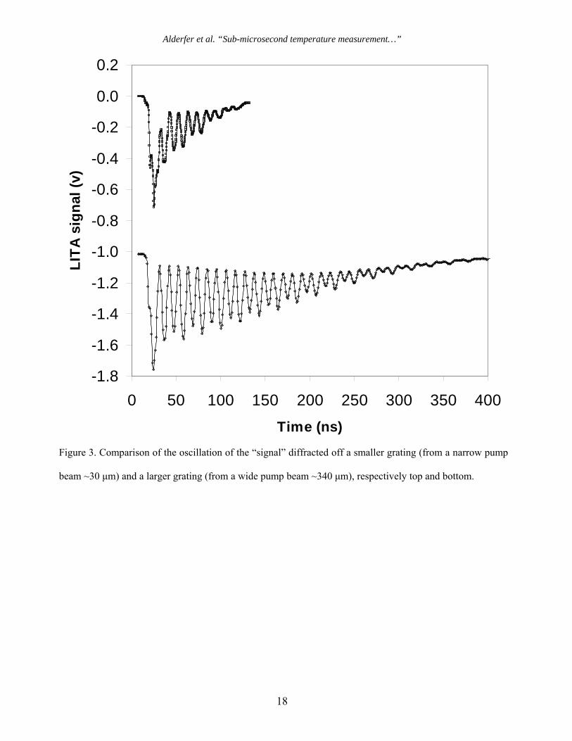
The number of observed oscillations of the signal is dependent on the wavelength of the

laser, the crossing angle (see Equation 2), the three input beam diameters; the shape of the decay

is a function of the size of the interaction region and the acoustic-decay properties of the

medium. The effect of the pump-beam diameter is shown in Figure 3. Both signal traces, in

Figure 3, are produced using 532-nm laser beams crossed at about 1 deg. In the top signal trace,

the pump beams (about 1-cm diameter) are not apertured before the focusing lens, resulting in a

calculated pump beam width and height of approximately 50 x 50 um in the interaction region.

About 8 oscillations occur in this configuration.

For the bottom trace, we inserted a 4.5 mm internal diameter stainless steel flat washer into

the pump beam before the 50/50 beam splitter and then rotated the washer nearly 70 deg about

the vertical axis, effectively aperturing the pump beams, mainly in the horizontal dimension.

Thus, in the interaction region, the calculated diffraction spreads the horizontal pump-beam

width to about 250 μm, but leaves the vertical portion only slightly larger - about 110 μm. This

effect increased the number of oscillations to approximately 30. Not only did spreading the

beam width at the crossing point create more oscillations, making the frequency determination

more accurate, but it also reduced the pump-beam peak intensity which had the effect of


9

reducing stimulated Raman interference and the probability for laser-induced breakdown in the

focal region.

Each single-shot temperature measurement consisted of 500 temporal points digitized at 1

GHz. Mean temperatures were determined by averaging the temperatures determined from

either 100 or 125 laser shots. We obtained 56 averaged measurements at various temperatures

between 10 – 75 °C. A LabVIEW curve-fitting algorithm was used to fit the data to an

empirical equation involving the sums of exponentially-damped sine waves. This empirical

model was not an accurate physical model of the LITA signal, but gave quick and accurate

determinations of the LITA signal modulation frequency. Data that were determined to be errant

(outliers) were discarded when the signal amplitude was below threshold (< 20% of average

signal amplitude). Data below threshold level consisted of less than 10% of the total data. A fast

Fourier transform (FFT) algorithm was also used to determine the signal modulation frequencies,

but was found to produce larger root-mean-square (RMS) fluctuations.

5. Results

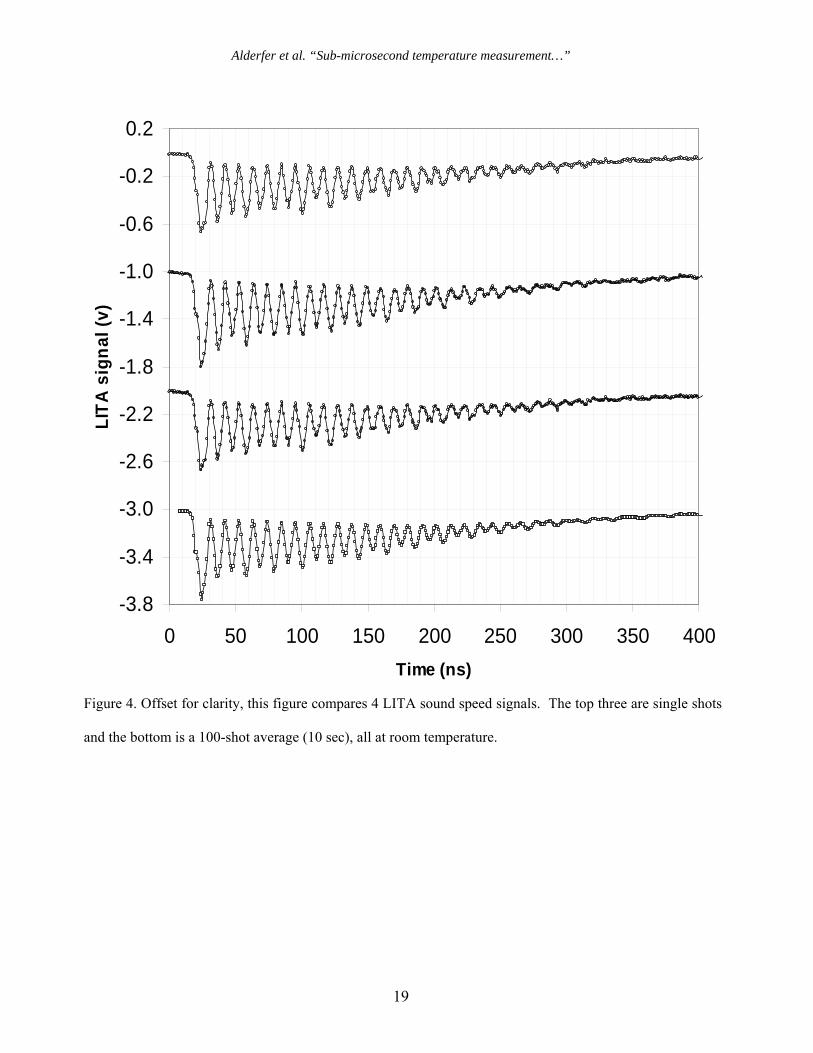
A comparison of three single shots and a 100-shot average measurement, taken at room

temperature, is shown in Figure 4. The traces show the characteristic oscillations associated with

dynamic diffraction gratings caused by the counter-propagating acoustic waves. They also show

the exponential-like decay caused by the combination of the acoustic dissipation and the acoustic

waves passing out of the probe volume. The first three traces are single-shot acquisitions and the

fourth trace is an average of 100 single-shot acquisitions. The data has been offset for

comparison. The quality and SNR for the single-shot signals compare well with the 100-shot

average, making single-shot measurements very practicable. Also, alternating valley heights

(particularly evident in the bottom averaged signal) indicate a small contribution from thermal


10

gratings. See Cummings for discussion on thermal and electrostriction contributions.17 We

believe that this is caused by a small amount of absorption of the 532-nm pump beams in water

of approximately 0.0004 cm-1.19 However, impurities in the water could also be absorbing some

of the laser energy.

The large SNR of the single-shot measurements is very important for making temperature

measurements that are accurate and fast. Less precise determination of the frequency could

reasonably be made in much less than 300 ns (e.g., three oscillations over 30 ns) with the data

shown in Figure 4, since only a few oscillations are needed for FFT or curve-fit analysis. Thus

we could, in principle, have made 30-ns measurements, albeit with larger uncertainties than we

are quoting below, instead of 300-ns measurements. Since the frequency of the oscillation is

governed by the crossing angle of the pump beams, increasing the pump-beam crossing angle

could also, potentially, improve the measurement quality or shorten the measurement time.

Caution is required to keep the period of the acoustical oscillations longer than the duration of

the pump-laser pulse; otherwise the grating would be washed out. This was a limiting factor in

the present experiment. It limited our pump beam total crossing angle to about 2 ° or less.

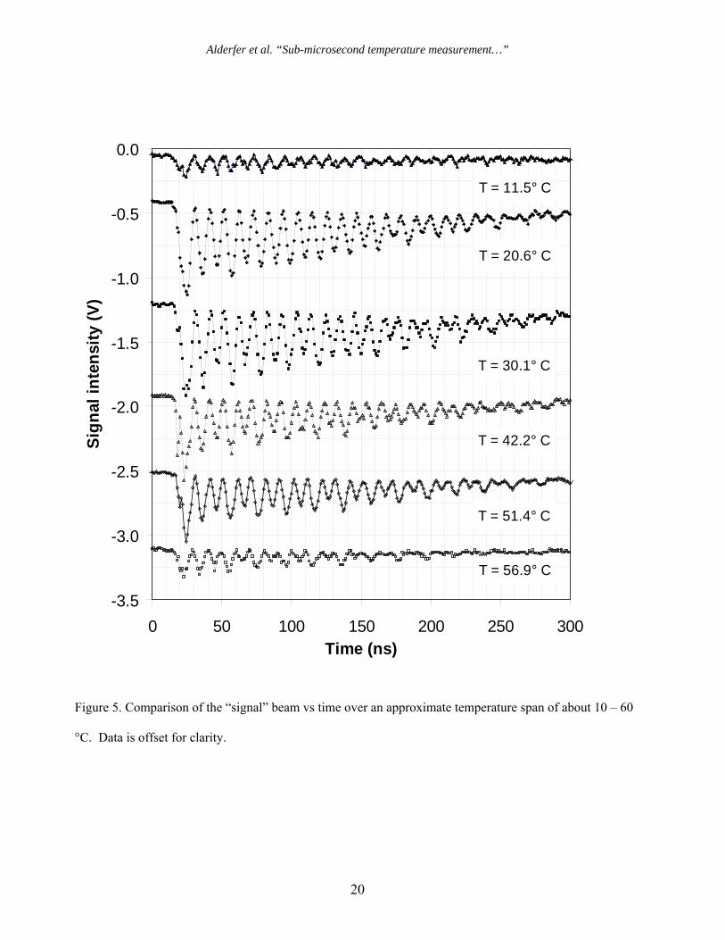
In Figure 5, single-shot LITA acoustic frequency traces are plotted as a function of time for

six different temperatures between 10 – 60 °C. Upon careful inspection, the oscillation

frequency is observed to increase with temperature. The SNR degrades as the temperature is

varied away from room temperature. There are several reasons for this. The system was aligned

and the crossing angle was calibrated at a room temperature of about 17 °C. As the temperature

was changed from ambient, temperature gradients were formed in the water, due to minimal

insulation around the water oven. This natural convection produced time-dependent beam

steering for the three input laser beams and the diffracted signal beam. This beam steering could


11

change the crossing angle and thus the measured frequency. Furthermore, it could cause the

overlap of the beams to not be optimal. Beam steering also caused the diffracted signal beam to

move with respect to the pinhole that was used as a spatial filter, hence changing the

transmission of the signal through the pinhole. The effects of the temperature gradients

worsened with increasing temperature deviation from ambient. Despite the problems with beam

steering, the LITA sound speed measurement technique produced accurate and precise sound

speed measurements over the range 10 - 45 °C.

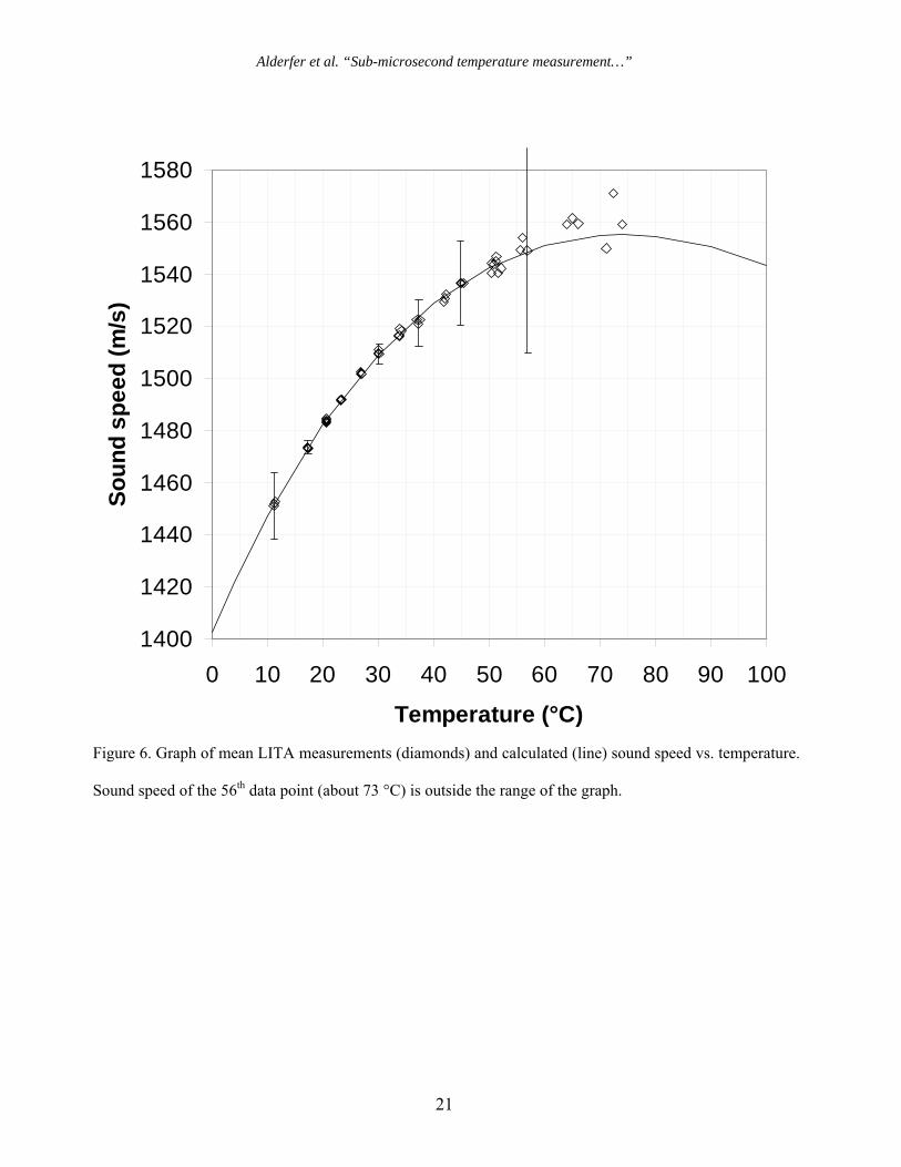
Figure 6 shows a simultaneous plot of calculated sound speed and 56 LITA mean sound

speed measurements versus temperature. Of these 56 measurements, 40 were in the range 10 –

45 °C. In this temperature range, the averaged accuracy of the mean sound speed measurements

was 0.64 m/s. Here, the averaged accuracy is defined as the averaged absolute difference

between the LITA sound speed measurement and the calculated sound speed. The precision of

single-shot measurements (based on 1 σ, or standard deviation of ≥100 samples) ranged from 1

m/s to 16.5 m/s. The error bars plotted are ± 1 σ. The uncertainties in these mean values (not

plotted) are about 10 times smaller than these plotted error bars, owing to the averaging of ≥ 100

measurements. As can be seen from the data and selected error bars on the plot, the scatter

appears to increase with deviation from room temperature. This suggests that beam steering is a

major contributor to the decreasing SNR with variance from room temperature. In situations

without the strong thermal gradients and beam steering, as in our current experiment, one could

reasonably expect somewhat better results than that shown at the higher temperatures of Figure

6.

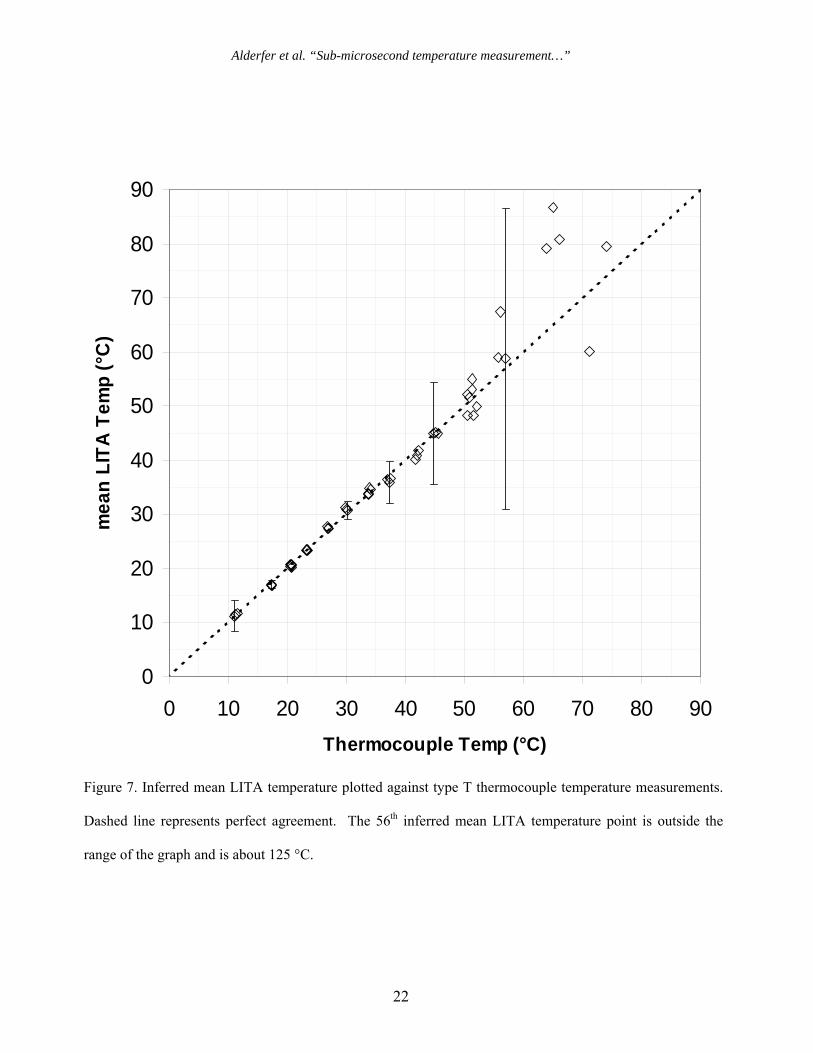
In Figure 7, 55 of the mean LITA temperatures inferred from the 56 LITA sound speed

measurements of Figure 6 are plotted against simultaneous thermocouple temperature


12

measurements. The thermocouple was located approximately 6 mm above the LITA temperature

measurement location. The 56th LITA temperature was, anomalously, determined to be about

125 °C when the thermocouple read 73 °C, and lies outside the range of Figure 7. The dashed

diagonal line represents perfect agreement between the LITA measurement and the

thermocouple measurement. The figure shows very good agreement between LITA-measured

temperature and the thermocouple in the region 10 – 45 °C. In this region, the averaged

accuracy of the LITA single shot temperature measurements was 0.45 °C and the single shot

precisions (based on 1 σ of > 100 shots) of the temperature measurements range from 0.3 °C to

9.5 °C. Here averaged accuracy is defined as the averaged absolute difference between the LITA

inferred temperature measurement and the thermocouple temperature measurement. Due to the

sound speed maximum at about 75°C, the measured LITA temperatures approaching 75 °C

become inaccurate.

6. Conclusion

We have made non-intrusive sound speed and temperature measurements in pure liquid

water over a range 10 – 75 °C in less than 300 nanoseconds per measurement using LITA. In the

range of 10 – 45 °C, the averaged accuracy of mean sound speed measurements was 0.64 m/s

and single shot precisions (1 σ) ranged from 1 m/s to 16.5 m/s. The averaged accuracy of the

LITA inferred mean temperatures over the same range was 0.45 °C and the single shot precisions

(1 σ) ranged from 0.3 °C to 9.5 °C. While LITA temperature measurements have been made

previously in various gases, we believe that this is the first time that this technique has been

extended to the sound speed and temperature measurement of liquids. It is our belief that this

technique will have future potential for making spatially-precise, non-intrusive, accurate and

precise temperature measurements in water for a wide spectrum of experiments, especially the


13

study of shock waves in water for bio-medical applications. This technique is preferred over the

other techniques mentioned because of the coherent nature of the signal beam, which allows for

fast single-shot acquisitions that are accurate and precise.

Our study proved that making fast (300 ns), accurate, spatially resolved (.1 x 0.25 x 30

mm3),[height x width x length] and non-intrusive temperature measurements in water is possible.

Using an improved LITA system, with a shorter pulse duration (a few hundred pico-seconds)

laser and crossing the pump beams with a larger angle, faster temperature measurements with

much better spatial resolution may be possible. In addition, liquids other than water, that also

simulate the acoustic properties of body fluids, may provide a larger usable temperature range.

Acknowledgement

We wish to thank Stephen B. Jones for his expertise in setting up the laboratory and

equipment and for his timely advice on optics design.


14

References

1. S. Hayakawa, K. Takayama, “Shock wave propagation in model tissue for medical

application of shock waves,” International Symposium on Shock Waves 21, Paper 5836,

(1997).

2. K. Nagayama, Y. Mori, K. Shimada, M. Nakahara, “Shock hugoniot compression curve for

water up to 1 GPa by using a compressed gas gun,” J. of Appl. Phys. 91, 476-482 (2002).

3. Kazuyoshi Takayama, “Applications of shock wave research to medicine,” International

Symposium on Shock Waves 22, Paper 2010 (1999).

4. G. A. Lyzenga, Thomas J. Ahrens, W. J. Nellis, A. C. Mitchell, “The temperature of shock-

compressed water,” J. Chem. Phys. 76, (1982).

5. N. C. Holmes, R. Chau, “Fast time-resolved spectroscopy in shock compressed matter,” J.

Chem. Phys. 119, 3316-3319, (2003).

6. J. Karl and D. Hein, “Measuring water temperature profiles at stratified flow by means of

linear raman spectroscopy,” Proceedings 2nd Japanese German Symp. on Multi-Phase Flow,

Tokyo University, Tokyo, Japan (1997).

7. Jianfeng Lou, Timothy M. Finegan, Paulash Mohsen, T. Alan Hatton, and Paul E. Laibinis

“Fluorescence-based thermometry: principles and applications,” Reviews In Analytical

Chemistry 18, 235-284 (1999).

8. Edward S. Fry, Jeffrey Katz, Dahe Liu, Thomas Walther, “Temperature dependence of the

brillouin linewidth in water” J. of Mod. Opt, 49, 411-418 (2002).

9. Eric B. Cummings, Hans G. Hornung, Michael S. Brown, and Peter A. DeBarber,

“Measurement of gas-phase sound speed and thermal diffusivity over a broad pressure range

using laser-induced thermal acoustics,” Opt. Lett. 20, 1577-1579 (1995).


15

10. Roger C. Hart, R. Jeffrey Balla, and G. C. Herring, “Optical measurement of the speed of

sound in air over the temperature range 300-650 K,” J. Acoust. Soc. Am. 108, 1946-1948 (2000).

11. A. Stampanoni-Panariello, B. Hemmerling, and W. Hubschmid, “Temperature

measurements in gases using laser induced electrostrictive gratings,” Appl. Phys. B 67, 125-130

(1998).

12. Michael S. Brown and William L. Roberts, “Single-point thermometry in high-pressure,

sooting, premixed combustion environments,” J. Propulsion Power 15 (No 1), 119-127 (1999).

13. Roger C. Hart, R. Jeffrey Balla, and G. C. Herring, “Nonresonant referenced laser-induced

thermal acoustics thermometry in air,” Appl. Opt. 38, 577-584 (1999).

14. Y. Nagasaka, T. Hatakeyama, M. Okuda, and A. Nagashima, “Measurement of the thermal

diffusivity of liquids by the forced Rayleigh scattering method: Theory and experiment,” Rev.

Sci. Instrum. 59, 1156-1168 (1988).

15. Alexei A. Maznev, Daniel J. McAuliffe, Apostolos G. Doukas and Keith A. Nelson, “Wide-

band acoustic spectroscopy of biological material based on a laser-induced grating technique,”

Ultrasound in Med. & Biol. 25, 601-607 (1999).

16. H. J. Eichler, P. Günter, D. W. Pohl, “Production and Detection of Dynamic Gratings,” in

Laser-Induced Dynamic Gratings, (Springer-Verlag, Berlin, Heidelberg, 1986), pp. 13-37.

17. E. B. Cummings, I. A. Leyva, and H. G. Hornung, “Laser-induced thermal acoustics (LITA)

signals from finite beams,” Appl. Opt. 34, 3290-3302 (1995).

18. Martín Chávez, Victor Sosa, and Ricardo Tsumura, “Speed of sound in saturated pure

water,” J. Acoust. Soc. Am. 77, 420-423 (1985).

19. George M. Hale and Marvin R. Querry, “Optical constants of water in the 200-nm to 200-

μm wavelength region,” Appl. Opt. 12, 555-563 (1973).


16

1400

1420

1440

1460

1480

1500

1520

1540

1560

1580

0 10 20 30 40 50 60 70 80 90 100

Temperature (°C)

Sou

nd s

peed

(m/s

)

1400

1420

1440

1460

1480

1500

1520

1540

1560

1580

0 10 20 30 40 50 60 70 80 90 100

Temperature (°C)

Sou

nd s

peed

(m/s

)

Figure 1. Visual demonstration of how temperature is inferred from LITA sound speed measurements, and how,

for a constant sound speed uncertainty (constant distance between horizontal lines), temperature uncertainty

increases with temperature (increasing distance between vertical lines with increase with temperature).


17

Figure 2. Diagram of the LITA experiment. Grating and probe generating optics are on the left side of the

test cell and collection/reading optics are shown on the right side of the test cell.

PMTOscilloscope

Test Cell

PathLengthmatcher

Nd:YAG Laser

Argon-Ion Laser

lens BeamDump

lens

Fiber Optic

532 nm

488 nm

Water

Pinhole

attenuator


18

Figure 3. Comparison of the oscillation of the “signal” diffracted off a smaller grating (from a narrow pump

beam ~30 μm) and a larger grating (from a wide pump beam ~340 μm), respectively top and bottom.

-1.8

-1.6

-1.4

-1.2

-1.0

-0.8

-0.6

-0.4

-0.2

0.0

0.2

0 50 100 150 200 250 300 350 400

Time (ns)

LITA

sig

nal (

v)


19

Figure 4. Offset for clarity, this figure compares 4 LITA sound speed signals. The top three are single shots

and the bottom is a 100-shot average (10 sec), all at room temperature.

-3.8

-3.4

-3.0

-2.6

-2.2

-1.8

-1.4

-1.0

-0.6

-0.2

0.2

0 50 100 150 200 250 300 350 400Time (ns)

LITA

sig

nal (

v)


20

-3.5

-3.0

-2.5

-2.0

-1.5

-1.0

-0.5

0.0

0 50 100 150 200 250 300Time (ns)

Sign

al in

tens

ity (V

)

T = 11.5° C

T = 20.6° C

T = 30.1° C

T = 42.2° C

T = 51.4° C

T = 56.9° C

Figure 5. Comparison of the “signal” beam vs time over an approximate temperature span of about 10 – 60

°C. Data is offset for clarity.


21

Figure 6. Graph of mean LITA measurements (diamonds) and calculated (line) sound speed vs. temperature.

Sound speed of the 56th data point (about 73 °C) is outside the range of the graph.

1400

1420

1440

1460

1480

1500

1520

1540

1560

1580

0 10 20 30 40 50 60 70 80 90 100

Temperature (°C)

Soun

d sp

eed

(m/s

)


22

Figure 7. Inferred mean LITA temperature plotted against type T thermocouple temperature measurements.

Dashed line represents perfect agreement. The 56th inferred mean LITA temperature point is outside the

range of the graph and is about 125 °C.

0

10

20

30

40

50

60

70

80

90

0 10 20 30 40 50 60 70 80 90Thermocouple Temp (°C)

mea

n LI

TA T

emp

(°C

)

Sub-microsecond temperature measurement in … be submitted to Applied Optics 1 Sub-microsecond...

Documents

Transcript of Sub-microsecond temperature measurement in … be submitted to Applied Optics 1 Sub-microsecond...