Structural Reliability Analysis of Complex Systems ...
146
Sede Amministrativa: Università degli Studi di Padova Dipartimento di Ingegneria Industriale _______________________________________________________________________ SCUOLA DI DOTTORATO DI RICERCA IN: Scienze Tecnologie e Misure Spaziali INDIRIZZO: Scienze e Tecnologie per Applicazioni Satellitari e Aeronautiche CICLO XXVII Structural Reliability Analysis of Complex Systems: Applications to Offshore and Composite Structures Direttore della Scuola: Ch.mo Prof. Giampiero Naletto Coordinatore d’indirizzo: Ch.mo Prof. Giampiero Naletto Supervisore: Ch.mo Prof. Ugo Galvanetto Dottorando: Marco Nicolò Coccon
Transcript of Structural Reliability Analysis of Complex Systems ...

Sede Amministrativa: Università degli Studi di Padova
Dipartimento di Ingegneria Industriale_______________________________________________________________________
SCUOLA DI DOTTORATO DI RICERCA IN: Scienze Tecnologie e Misure Spaziali
INDIRIZZO: Scienze e Tecnologie per Applicazioni Satellitari e Aeronautiche
CICLO XXVII
Structural Reliability Analysis of Complex Systems:
Applications to Offshore and Composite Structures
Direttore della Scuola: Ch.mo Prof. Giampiero Naletto
Coordinatore d’indirizzo: Ch.mo Prof. Giampiero Naletto
Supervisore: Ch.mo Prof. Ugo Galvanetto
Dottorando: Marco Nicolò Coccon


ii
Summary
This thesis aims at developing new methodologies for the reliability analysis of
structural systems with applications to offshore and aeronautical fields. In general, sructures
of practical interest are complex redundant systems, in which more than one element is
required to fail in order to have catastrophic failure. Moreover, ramdomness inherently exists
in both material properties and external loads. As a result, complex structural systems are
typically characterised by a huge number of possible failure sequences, of which only some
are most likely to occour. Therefore, for an efficient risk analysis, only the dominant failure
modes need to be considered, so as to minimise the number of failure paths as well as the
computational costs associated to their enumeration and evaluation. However, although
several techniques have been developed for the identification of the critical failure sequences,
these methods are still either time-demanding or prone to miss potential failure modes.
These challenges motivated the first part of the thesis, in which the merits of a risk
assessment framework recently developed for truss and frame structures are here investigated
in view of its extensive application to the offshore field. To this end, the case study of a
jacket-type platform under an extreme sea state is considered. First, the dominant failure
modes of the structure are rapidly identified by a multi-point parallel search employing a
genetic algorithm. Then, a multi-scale system reliability analysis is performed, in which the
statistical dependence among both structural elements and failure modes is fully considered
through simple matrix operations. Finally, the accuracy and the efficiency of the proposed
approach are successfully validated against crude Monte Carlo simulation.
In the second part of the thesis, system reliability theory is applied to the uncertainty
quantification of the longitudinal tensile strength of UniDirectional (UD) composites, a
structural component very common in aircraft structures. Predictive models for size effects in
this class of materials are paramount for scaling small-coupon experimental results to the
design of large composite structures. In this respect, a Monte Carlo progressive failure
analysis is proposed to calculate the strength distributions of hierarchical fibre bundles, which
are formed by grouping a predefined number of smaller-order bundles into a larger-order one.
The present approach is firstly validated against a recent analytical model to be later applied
to more complex load-sharing configurations. The resulting distributions are finally used to
analyse the damage accumulation process and the formation of clusters of broken fibres
during progressive failure.


iv
Sommario
Lo scopo principale di questa tesi è lo sviluppo di nuove metodologie per determinare
l’affidabilità dei sistemi strutturali con applicazioni sia in campo offshore che aeronautico. In
generale, strutture di interesse pratico sono caratterizzate da un elevato grado di ridondanza,
per cui il collasso globale richiede la rottura simulatanea e/o progressiva di più elementi.
Inoltre, i sistemi fisici sono influenzati da diverse fonti di incertezza, quali le prorietà dei
materiali e le condizioni ambientali e operative. Pertanto, il collasso strutturale può avvenire
con diverse modalità (modi di guasto), di cui solo alcune possiedono una probabilità di
accadimento significativa (modi di guasto dominanti). Per una valutazione efficiente del
rischio risulta dunque indispensabile limitare l’analisi ai soli modi dominanti, così da ridurre
il costo computazionale associato alle fasi di identificazione e di valutazione dei modi stessi.
Tuttavia, nonostante in letteratura vi siano numerose soluzioni per l’analisi del rischio, tali
metodi richiedono ancora tempi di calcolo notevoli e sono inclini a tralasciare potenziali modi
di guasto.
Queste motivazioni conducono alla prima parte delle tesi, in cui si ripropone un
metodo recentemente sviluppato per l’analisi del rischio di strutture discrete (reticolari e telai)
in previsione di una sua applicazione al campo offshore. A tale scopo si considera il caso di
studio di una piattaforma di tipo jacket in condizioni di mare estremo. Dapprima, i modi di
guasto dominanti vengono rapidamente identificati per mezzo di un algoritmo genetico. In
seguito, l’affidabilità del sistema viene calcolata mediante un approccio multi-scala che fa uso
di semplici operazioni matriciali, in cui la dipendenza statistica viene considerata sia tra le
componenti strutturali che tra i modi di guasto dominanti. Infine, l’accuratezza e l’efficienza
del metodo vengono testate con successo tramite comparazione con Monte Carlo.
Nella seconda parte della tesi, la teoria dell’affidabilità dei sistemi viene applicata per
la quantificazione dell’incertezza nella resistenza a trazione di compositi UniDirezionali
(UD), problema di notevole interesse per l’ambito aeronautico e non solo. Infatti, il
comportamento aletorio di questi materiali è fortemente influenzato da effetti di scala, che
limitano la progettazione di strutture in composito di grandi dimensioni sulla base dei dati
sperimentali ricavati da provini. In quest’ottica, si propone di modellare fasci di fibre secondo
una legge di scala gerarchica, ossia raggruppando un numero prestabilito di fasci più piccoli
in un fascio di ordine superiore. La distribuzione di resistenza di tali fasci viene quindi
simulata attraverso un’analisi di collasso progressivo. Questo approccio, dapprima validato
rispetto ad un modello analitico recentemente sviluppato per disposizioni semplici di fasci,
viene poi esteso a configurazioni più realistiche. I risultati così ottenuti sono infine processati
per l’analisi statistica del danno.


vi
Acknowledgements
The research work in this thesis was mainly supported by EnginSoft S.p.A under a
cooperative agreement with the University of Padova (protocol number 42035, 09 Aug 2011).
Additional support was provided by Fondazione Ing. Aldo Gini and by the Italian Ministry of
Education, University and Research (MIUR) by the PRIN program 2010/11N.2010MBJK5B.
Firstly, I wish to express my sincere gratitude to my supervisor, Professor Ugo
Galvanetto. Since I started my Ph.D., he has given me passionate advice, continuous support
and encouragement. I am indebted to him for giving me the extraordinary opportunity to
develop my research at the University of Illinois at Urbana-Champaign and at Imperial
College London. Such experiences have been paramount in my professional and personal
growth, and I believe it was one of the best decisions of my life to join Professor Galvanetto’s
research group as a doctoral student.
I would like to thank Professor Junho Song for giving me the possibility to work in the
Department of Civil and Environmental Engineering at the University of Illinois at Urbana-
Champaign. I have learned so many things from him, and his guidance has been invaluable in
completing my research. I hope that we will be working on a joint project again.
Similarly, I would like to thank Dr. Soraia Pimenta for giving me the possibility to
work in the Department of Mechanical Engineering at Imperial College London. She has been
the perfect role model as a researcher, teacher, and person. I am also grateful to her for always
pushing me and giving me the critiques and the instructions I needed to make this work
something I am proud of.
I would also like to thank the former and current members of Professor Song’s
Structural System Reliability Group, Junho Chun, Nolan Kurtz, and Derya Deniz, as well as
the members of Dr. Pimenta’s research group, Gianmaria Bullegas, Cihan Kaboglu, and Gael
Grail. It was my great pleasure to share this time and have research discussions with them.
For all the moments of leisure and relaxation during the everyday difficulties of a
Ph.D. life, I would like to thank my officemates of “Room-308”, Tasnuva, Sherry, Farnaz,
Tom, Mitesh, James, Rodolfo, Christos, and, last but not least, my friend Michele. I would
also like to thank my colleagues from “CISAS”, Marco Thiene, Marco Menegozzo, Teo,
Daniele, Giulia, Arman, Siamak, and Lorenzo. To those I may have forgotten to mention, it is
pure lack of memory, and I send a great thank you to all of them.
A special thanks goes to Louis and Hannah for their great friendship. During my stay
at Urbana-Champaign, they have been like a second family to me. I will always remember the
happy moments we spent together with their adorable child, Johan.

I owe my loving thanks to my girlfriend Marta. She has been my world for nearly half
of my life, filling my days and supporting me throughout all the ups and downs during my
studies.
Finally, my deepest gratitude goes to my parents Francesco and Paola, who have
devoted their life to my sister Isabella and me. There are simply no words to express my
appreciation for all the love and support they have given us, and that I would never be able to
repay. To them I dedicate this thesis.

viii
Table of contents
SUMMARY............................................................................................................................. ii
SOMMARIO.......................................................................................................................... iv
ACKNOWLEDGEMENTS ................................................................................................ vi
TABLE OF CONTENTS ..................................................................................................viii
LIST OF FIGURES.............................................................................................................xii
LIST OF TABLES.............................................................................................................. xvi
1 INTRODUCTION ............................................................................................................ 1
1.1 MOTIVATION AND SCOPE OF THIS THESIS......................................................... 1
1.2 OUTLINE OF THIS THESIS ........................................................................................ 5
2 STRUCTURAL RELIABILITY THEORY ............................................................... 7
2.1 COMPONENT RELIABILITY ANALYSIS................................................................. 7
2.1.1 Fundamental concepts of reliability theory.......................................................... 7
2.1.2 Closed-form solution of the probability integral................................................ 11
2.1.3 Random variable transformations ...................................................................... 13
2.1.4 Toward an approximate calculation of the reliability index .............................. 16
2.1.5 First-Order Reliability Method (FORM) ........................................................... 18
2.1.6 The MPP search algorithm................................................................................. 21
2.1.7 Second-Order Reliability Method (SORM)....................................................... 24
2.1.8 Monte Carlo analysis ......................................................................................... 25
2.2 SYSTEM RELIABILITY ANALYSIS........................................................................ 30
2.2.1 Component and system failures ......................................................................... 30
2.2.2 Series systems .................................................................................................... 32
2.2.3 Parallel systems.................................................................................................. 34
2.2.4 General systems ................................................................................................. 36
3 RELIABILITY ANALYSIS OF OFFSHORE STRUCTURES.................................... 41
3.1 OCEAN ENVIRONMENT.......................................................................................... 41
3.1.1 Design approaches ............................................................................................. 41
3.1.2 Wave spectrum model........................................................................................ 43
3.1.3 Short-term design approach ............................................................................... 44

3.2 STRUCTURAL MODEL AND LOAD DEFINITION ............................................... 47
3.3 IDENTIFICATION OF THE DOMINANT FAILURE MODES................................ 52
3.4 SYSTEM RELIABILITY ANALYSIS........................................................................ 56
3.4.1 Matrix-based System Reliability (MSR) method............................................... 56
3.4.2 Multi-scale system reliability analysis framework ............................................ 61
3.5 RESULTS AND DISCUSSION................................................................................... 62
3.6 CONCLUSIONS .......................................................................................................... 69
4 SIMULATION OF THE LONGITUDINAL TENSILE STRENGTH AND
DAMAGE ACCUMULATION IN FIBRE-REINFORCED COMPOSITES... 71
4.1 SIZE EFFECTS............................................................................................................ 72
4.2 OVERVIEW OF THE HIERARCHICAL ANALYTICAL MODEL FOR
COMPOSITE FIBRE BUNDLES................................................................................ 75
4.2.1 Hierarchical scaling law for the bundle strengths .............................................. 75
4.2.2 Accumulation and clustering of fibre breaks ..................................................... 78
4.3 NUMERICAL IMPLEMENTATION.......................................................................... 80
4.3.1 Simulation of failure events in a bundle with 2 fibres ....................................... 80
4.3.2 Simulation of larger bundles and asymptotic analysis of the strength
distribution ......................................................................................................... 83
4.3.3 Extension of the numerical model to higher coordination numbers .................. 87
4.3.4 Optimal discretisation of the fibre bundles ........................................................ 89
4.4 RESULTS..................................................................................................................... 91
4.4.1 Inputs and outputs .............................................................................................. 91
4.4.2 Comparison between Monte Carlo analysis and the analytical model .............. 92
4.4.3 Effects of the coordination number.................................................................... 92
4.4.4 Analysis of damage accumulation ..................................................................... 95
4.5 DISCUSSION............................................................................................................... 98
4.5.1 Limitations of the present model ....................................................................... 98
4.5.2 Advantages of the present model ....................................................................... 99
4.6 CONCLUSIONS ........................................................................................................ 100
5 GENERAL CONCLUSIONS ..................................................................................... 103
5.1 SUMMARY OF MAJOR FINDINGS ....................................................................... 103
5.2 FUTURE RESEARCH TOPICS................................................................................ 105
REFERENCES................................................................................................................... 107

x
APPENDIX A: REGULAR WAVE THEORIES ....................................................... 115
APPENDIX B: DUNNETT-SOBEL CLASS CORRELATION MODEL............ 119
APPENDIX C: SYSTEM RELIABILITY ANALYSIS USING
MONTE CARLO ................................................................................. 123
APPENDIX D: DERIVATION OF THE HIERARCHICAL SCALING LAW 127


xii
List of figures
Figure 1.1: Jacket-type platform under an extreme sea loading. ............................................... 3
Figure 1.2: a) First 4 bundle levels with coordination number = 2; b) Fibre arrangements
for different coordination numbers. ........................................................................... 4
Figure 2.1: Geometrical interpretation of the convolution integral in Eq. (2.5). ....................... 9
Figure 2.2: Geometrical interpretation of the probability of failure ........................................ 10
Figure 2.3: Limit state equation and failure domain before (a) and after (b) transformation. . 11
Figure 2.4: Closed-form solution of the probability integral. .................................................. 13
Figure 2.5: Contour lines of a 2D joint PDF in the original space (a), in the correlated
standard normal space (b), and in the independent standard normal space (c).13
Figure 2.6: Actual limit state equation and linearised limit state equations. ........................... 17
Figure 2.7: Highest value of the joint PDF at the MPP (Du, 2015). ........................................ 19
Figure 2.8: Plan view of the integration domain in FORM (Du, 2015). .................................. 19
Figure 2.9: Relation among , the unit vector and the MPP vector . ........................... 20
Figure 2.10: The flowchart of the iHLRF algorithm................................................................ 23
Figure 2.11: Converge of crude Monte Carlo: coefficient of variation (full line) and estimated
error (dashed line). ................................................................................................ 27
Figure 2.12: Random points generated by MCS mapped into the standard normal space. ..... 27
Figure 2.13: Linear approximation operated by FORM. ......................................................... 29
Figure 2.14: Statically determinate truss structure................................................................... 30
Figure 2.15: System failure domain ( < 0) ( < 0). ..................................................... 31
Figure 2.16: Formation of a mechanism in a statically determinate structure (a), and
corresponding series system (b). ........................................................................... 32
Figure 2.17: Formation of a mechanism in a statically indeterminate structure (a) and
corresponding parallel system (b). ........................................................................ 34
Figure 2.18: Failure modes with respect to the frame structure in Figure 2.17. ...................... 36
Figure 2.19: a) Cut set = { , , , }: the system fails even if survives; b) Minimal
cut set = { , , }: if any element in survives, the system survives as well.
............................................................................................................................... 37
Figure 3.1: JONSWAP spectrum ( = 10 m, = 14 s). .................................................... 44
Figure 3.2: Statistical characterisation of the short-term sea state. .......................................... 47
Figure 3.3: Jacket-type platform. ............................................................................................. 48
Figure 3.4: Variation of the base shear force with the wave phase.......................................... 51
Figure 3.5: Distribution of the wave-current forces when wave phase is equal to -2 deg. ...... 51
Figure 3.6: Failure mode in standard normal random variable space (Kim et al., 2013)......... 52
Figure 3.7: Progressive failure analysis and formation of a mechanism after redistribution of
the internal load effects (T = tension failure, C = compression failure). ............. 53
Figure 3.8: Searching operations in GA by crossover and mutation operators........................ 54

Figure 3.9: Flowchart of the multi-point parallel searching method (Kim et al., 2013). ......... 55
Figure 3.10: Network representation of a system event consisting of two failure modes:
( and ) or . ................................................................................................. 57
Figure 3.11: Sample space for the three-component system in Figure 3.10. ........................ 59
Figure 3.12: a) Influence of the post-buckling factor on the system reliability; b) relative
errors between the proposed method (GA-MSR) and MCS. ................................ 64
Figure 3.13: Influence of the post-buckling factor on the computational costs of the
selective searching technique and MCS in terms of a) iteration number and b)
computational time. ............................................................................................... 65
Figure 3.14: Minimal cut set representation of the system failure event for = 0.5.............. 66
Figure 3.15: Horizontal component of wave-current load calculated at a) the node between
elements 15-16 (see Figure 3.3) and b) the node between elements 24-27........... 67
Figure 3.16: Minimal cut set representation of the system failure event for = 0.8.............. 68
Figure 4.1: Size effects on the fibre-strength distributions. ..................................................... 73
Figure 4.2: Fracture contours within a fibre bundle, at three different magnification levels
(Pimenta et al., 2010). ........................................................................................... 74
Figure 4.3: a) First 4 bundle levels with coordination number = 2; b) Fibre arrangements
for different coordination numbers........................................................................ 74
Figure 4.4: A first break occurs in the middle of fibre , the matrix yields plastically, and a
linear stress concentration applies to fibre (Pimenta & Pinho, 2013). .............. 76
Figure 4.5: Definition of the critical distance between fibre breaks: the bundle fails if fibre
breaks at a distance smaller than /2 = e from the break in fibre (Pimenta &
Pinho, 2013). ......................................................................................................... 76
Figure 4.6: Definition of the control region and fibre segments in a level-[1] bundle (Pimenta
& Pinho, 2013). ..................................................................................................... 76
Figure 4.7: Shear-lag boundary for square fibre arrangement (Pimenta & Pinho, 2013). ....... 78
Figure 4.8: Damaged level-[ + 1] bundle of length [ ]
, in which only one of the two level-
[ ] bundles withstands the external load................................................................ 79
Figure 4.9: a) Elements 6 and 8 of fibre and element 15 of fibre fail under the uniform
stress ; b) Resulting stress fields with recovery regions in red and stress
concentrations in green.......................................................................................... 81
Figure 4.10: Unstable failure (event ); the level-[1] bundle fails at the first iteration of the
progressive failure analysis when is equal to the strength value of the weakest
element (i.e., element 15 of fibre : after its failure, fibre does not survive the
stress concentrations in elements 15 and 16). Note the different values of strength
and stress in the vertical axes. ............................................................................... 82
Figure 4.11: Stable failure (event ); the bundle fails after three iterations (the last iteration is
highlighted in red colour). After element 6 of fibre fails, fibre survives the
stress concentrations until reaches the strength of element 7 of fibre . Note
the different values of strength and stress in the vertical axes. ............................. 82

xiv
Figure 4.12: Stable failure (event ); the bundle fails due to growth and coalescence of the
recovery regions between two previously formed breaks (in element 15 of fibre
and element 8 of fibre ). Note the different values of strength and stress in the
vertical axes. .......................................................................................................... 83
Figure 4.13: The WLT is applied to scale the bundle distribution from the full level-[1]
bundle length ( [ ]) to the level-[1] element length ( [ ]), so that the level-[1]
element strengths can be sampled for the analysis of the level-[2] bundle........... 83
Figure 4.14: a) The limited number of Monte Carlo analyses rounds up to 1 the right tail of
both the bundle strength (, [ ]
[ ], blue curve) and the element strength (
, [ ]
[ ],
black curve) distributions; the latter is fitted with the asymptotic distribution
(lim, [ ]
[ ]( ), red curve) provided by the WLT applied to the previous
level bundle (Eq. (4.23)); b) region from plot a) highlighted............................... 84
Figure 4.15: WLT applied to the single-fibre level (case for = = 2). ............................... 85
Figure 4.16: WLT applied to the previous-level bundle (case for = = 2). ........................ 85
Figure 4.17: a) Asymptotic analysis of the first 3 levels using the WLT applied to the single-
fibre level (dashed lines) and to the previous-bundle level (dotted lines); b) region
from plot a) highlighted......................................................................................... 86
Figure 4.18: a) Elements 4 and 15 of fibre , elements 8 and 12 of fibre , and element 14 of
fibre fail under uniform stress loading ; b) The whole bundle fails due to
non-equilibrium in elements 13 and 14 (dashed areas). ....................................... 88
Figure 4.19: Strategy for an optimal discretisation of the fibre bundles.................................. 89
Figure 4.20: Simulated bundle strength distributions from level [1] to level [15], and
comparison with Pimenta and Pinho’s (2013) model. .......................................... 91
Figure 4.21: Bundle strength size effects on the mean value (a) and on the CoV (b) for
coordination numbers ranging from 2 to 7, and comparison with Pimenta and
Pinho’s (2013) model. ........................................................................................... 93
Figure 4.22: Simulated number of broken level-[ ] clusters in the level-[10] bundle of length
= 10 mm, and comparison with Pimenta and Pinho’s (2013) model............... 95
Figure 4.23: Simulated number of broken fibres (a) and associated density (b) in the level-
[10] bundle of length = 10 mm, and comparison with Pimenta and Pinho’s
(2013) model. ........................................................................................................ 96
Figure 4.24: Simulated number of broken fibres in the largest cluster of the level-[10] bundle
of length = 10 mm, and comparison with Pimenta and Pinho’s (2013) model.
............................................................................................................................... 96
Figure 4.25: Density of fibre breaks and size of the largest cluster in bundles with equal
length = 10 mm and similar cross-sectional areas. .......................................... 97
Figure 4.26: Different load-sharing configurations for a bundle with 4 fibres. ....................... 98
Figure 4.27: Influence of the total number of broken fibres on the recovery length. ............ 101
Figure A.1: 2D wave motion over flat bottom. ...................................................................... 116
Figure A.2: The range of validity of various wave theories (WAVE User Manual, 2010). .. 117

Figure C.1: Series systems consisting of two structural components. ................................... 123
Figure C.2: Sample space for the bicomponent system in Figure C.1................................ 124
Figure D.1: Definition of fibre segments in a level-[1] bundle (Pimenta & Pinho, 2013). ... 127

xvi
List of tables
Table 2.1: FERUM output file relative to FORM and SORM analyses. ................................. 28
Table 2.2: Percentage errors with the respect to the reliability index provided by MCS. ....... 28
Table 2.3: Iteration points of the MPP search by iHLRF......................................................... 29
Table 3.1: Geometrical and material properties of members. .................................................. 48
Table 3.2: Statistical properties of current speed and drag and mass coefficients................... 49
Table 3.3: Basic MECE events for the three-component system in Figure 3.10. .................... 57
Table 3.4: Results comparison between the selective searching technique and MCS............. 64
Table 3.5: Comparison of the computational costs required by the selective searching
technique and MCS. .............................................................................................. 65
Table 3.6: Failure modes and corresponding reliability indexes for = 0.5: a) Results
provided by MSR performing FORM compared to MCS; and b) results provided
by MSR performing SORM compared to MCS.................................................... 67
Table 3.7: Failure modes and corresponding reliability indexes for = 0.8: a) Results
provided by MSR performing FORM compared to MCS; and b) results provided
by MSR performing SORM compared to MCS.................................................... 68
Table 4.1: Input parameters for the numerical implementation. .............................................. 91
Table 4.2: Optimal discretisation of fibre bundles and convergence to the WLT for different
values of the coordination number. ....................................................................... 94


1
1 Introduction
1.1 Motivation and scope of this thesis
Since the late 1960s, structural reliability theory has been extensively applied to the
analysis, design and maintenance of structural systems in civil, nuclear, offshore and
aerospace fields (Frangopol & Maute, 2003; Haldar, 2006; Moan, 1994, 2005; Thoft-
Cristensen, 1998). In particular, most of the reliability applications have been primarily aimed
at developing limit state design formats, e.g., the North American codes for steel structures
(AISC), movable highway bridges (AASHTO), and offshore platforms (API RP2A). Such
specifications are mainly component-based with the underlying hypothesis that a structural
system will be safe as long as all its members are safe according to the corresponding limit
state equations. Hence, most research has been focusing on component reliability analysis
over the years, where a single limit state function is used to describe the failure event of
interest (e.g., overload, buckling or fatigue failure of a member). As a consequence, ensuring
pre-established target reliabilities to structural components became a part of everyday
common practice, but the calculation of the probability of a system-level failure (e.g.,
sequence of member failures leading to structural collapse) still poses very difficult
theoretical and practical challenges.
However, it has been increasingly recognized over the last few decades that system
reliability analysis is a matter of primary importance in the field of structural engineering.
First of all, it should be noted that the overall reliability of real structures is typically different
from the calibrated component reliabilities provided by present day design codes. In fact,
structures of practical interest are generally complex redundant systems, in which more than
one element is required to fail in order to have system-level failure. This is due to the residual
strength provided by non-failed elements, which resist the external loads by redistribution of
the internal load effects. Some effort has been made in present day design codes to account
for such system reserve strength. For instance, a simplified system approach has been
developed by the Joint Industry Project (JIP) (Bomel Ltd., 2002) to derive environmental load
factors for fixed steel offshore structures. Here, the calibration process is carried out on a
global failure function defined by the difference between the structural reserve strength and
the environmental load, in which the reserve strength is evaluated by deterministic
Introduction
2
progressive failure analyses. Nevertheless, from a reliability viewpoint this approach is still
component-based, since a single limit state equation is involved in the definition of the system
failure. In a similar way, a single-function event is often used to model the system failure of
offshore structures under extreme sea loading, where both the load and resistance terms in the
limit state equation are referred to as the overall base shear. Although this approach is
computationally efficient and particularly attractive for planning of inspection, maintenance
and repair strategies (Ayala-Uraga & Moan, 2002), it has been validated only for cases where
the load uncertainties are dominant and the resulting stresses in the components are highly
correlated (Wu & Moan, 1989). Such an assumption may not be true, as in the case of fatigue
failure, where the uncertainties related to resistance properties are higher and the correlation
among components is lower. Thus, it is clear that a more general and rigorous risk assessment
framework employing system-based reliability analysis is needed, in which the reliability of a
structural system is estimated with respect to all its potential (or dominant) failure modes and
their statistical dependence.
In general, complex structural systems are characterised by a huge number of critical
sequences of component failures leading to a system failure, of which only some (i.e., the
dominant failure modes) are most likely to contribute to the overall failure. Therefore, for an
efficient risk analysis, only the dominant failure modes need to be considered so as to
minimise the number of failure paths as well as the computational costs associated to their
enumeration and evaluation. Although several techniques have been developed for the
identification of the critical failure sequences (see review from Karamchandani, Dalane &
Bjerager, 1992), these methods are still either time-demanding or likely to miss potential
failure modes. In the latter case, the risk is underestimated due to heuristic rules that are often
introduced to improve the efficiency of the enumeration process. Concerning the evaluation
of the system failure probability, various approximate techniques have been proposed such as
the first-order system reliability method (Hohenbichler & Rackwitz, 1983) that applies
component reliability analyses to series and parallel systems directly, while it involves
theoretical bounding formulas (Ditlevsen, 1979) in the case of more complex systems. These
approaches are not flexible in incorporating various types and amount of available
information on components and their statistical dependence (Song & Kang, 2009). Moreover,
the complexity of a system event complicates the reliability computations and may require
overwhelming time costs.
These challenges motivated the first part of the present research, which aims to
investigate and develop new methodologies for the system reliability analysis of offshore
structures. A powerful risk assessment methodology has been recently developed for truss and
frame structures (Kim et al., 2013; Kurtz et al., 2010). Differently from standard probabilistic
approaches (Karamchandani, 1987; Lee & Song 2011, 2012; Murotsu et al., 1984; Thoft-
Christensen & Murotsu, 1986), the proposed method offers the main advantage that the
identification process of dominant failure modes is decoupled from the evaluation process of
their probabilities. In this way, the approach avoids performing reliability analyses repeatedly

Chapter 1
3
during the identification process, which otherwise may lead to huge computational costs
especially for large and highly-redundant structures. Here, the dominant failure modes are
rapidly identified in the decreasing order of their likelihood by means of a multi-point parallel
search employing a genetic algorithm. Once the identification phase is completed, the system
failure probability is evaluated by a multi-scale analysis employing the matrix-based system
reliability method (MSR) (Kang et al., 2012; Kang, Song & Gardoni, 2008; Lee et al., 2011;
Nguyen, Song & Paulino, 2010, 2011; Song and Kang 2009; Song and Ok, 2010), which has
been recently developed for accurate and efficient system reliability analysis through simple
matrix operations.
Figure 1.1: Jacket-type platform under an extreme sea loading.
In order to investigate the applicability of the proposed method to the risk assessment
of offshore structures, the case study of a jacket-type platform under an extreme sea loading is
considered (see Figure 1.1). Following the procedure adopted in (Thoft-Christensen &
Murotsu, 1986), the probabilistic model of the extreme sea loading is derived from a short-
term design storm, in which uncertainties are assumed both in the wave model (i.e., in the
wave height and the current speed) and the hydrodynamic model (i.e., in the drag and mass
coefficients of the tubular members). The structure is analysed as a truss and a further source
of uncertainty affects the yield stress of the members, which are assumed to fail either in
tension or compression. Nonlinearities on the structural response are mainly due to the top
side of the structure (the deck), which causes a sharp increase in wave-current forces as soon
as the wave height exceeds a certain value. Further nonlinear contributions arise from the
hydrodynamic model and the post-failure behaviour of the members, which is assumed purely
ductile in tension and brittle-ductile in compression. In particular, the effect of the post-
buckling factor on the redundancy of the structure is also investigated.
WAVE
DECK
JACKET

Introduction
4
In the second part of this thesis, system reliability theory is applied to the uncertainty
quantification of the longitudinal tensile strength of UniDirectional (UD) composites, a
structural component very common in aircraft structures. The damage accumulation and
failure of this class of materials is governed by statistical size effects, which pose a challenge
to use coupon-based experimental data for the design of large structures. Although most
authors agree that the statistics of fibre strength are essential for establishing the relationship
between composite longitudinal tensile strength and size effects, a widely accepted strategy
for the stochastic analysis of Fibre-Reinforced Polymers (FRPs) is still to be developed
(Wisnom, 1999).
Pimenta and Pinho (2013) recently proposed a hierarchical scaling law for the strength
of composite fibre bundles, which has been extensively validated against experimental results
and predicts full strength distributions for bundles of any size. As illustrated in Figure 1.2a,
the model assumes that hierarchical bundles are formed by grouping two smaller-order
bundles into a larger-order bundle (i.e., a coordination number = 2 is used). Once a sub-
bundle fails, stresses are recovered according to a plastic shear-lag model, so that linear stress
concentrations apply in the surrounding intact sub-bundle. Although this approach leads to an
efficient computation of bundle strength distributions, imposing a coordination number equal
to two results in very high stress concentrations in the proximity of fibre breaks.
Figure 1.2: a) First 4 bundle levels with coordination number = 2; b) Fibre arrangements
for different coordination numbers.
The objective of the present work is therefore to extend Pimenta and Pinho’s (2013)
model to more realistic load-sharing configurations, generalising the hierarchical approach to
higher coordination numbers (Figure 1.2b) and, consequently, reducing stress concentration
factors in the neighbourhood of fibre breaks. However, at higher coordination numbers, the
increasing number of possible sequences of failure events in a bundle complicates the
a)
b)

Chapter 1
5
analytical evaluation of its strength distribution and, thus, a new numerical approach is
needed. In this work, a Monte Carlo progressive failure analysis is proposed to calculate the
bundle strength distributions, where the failure events are simulated through a discrete
representation of hierarchical bundles. The damage accumulation into clusters of fibre breaks
is also investigated.
1.2 Outline of this thesis
This thesis is divided into five chapters, which can be summarised as follows:
Chapter 2 serves as an introduction to the system reliability theory. The probabilistic
concept of reliability is first introduced at the component level. First, a closed-form
solution is derived for the failure probability associated to linear limit state functions and
normal random variables. Second, the general case of non-linear limit state functions and
arbitrary distributions is addressed by means of approximate techniques, such as first-
and second-order reliability methods (FORM and SORM), and Monte Carlo simulation
(MCS). Lastly, the concept of reliability is extended to the system level, providing the
basic mathematical tools for the applications in Chapters 3 and 4.
Chapter 3 proposes a novel strategy for the risk assessment of offshore structures. The
genetic algorithm developed by Kim et al. (2013) is here combined with the MSR method
(Song & Kang, 2009) and applied to the analysis of a jacket platform under an extreme
sea state. First, the structural model and the loading conditions are derived, providing the
input random variables for the multi-point parallel search. Second, the main steps of the
failure mode identification process are summarised, followed by a detailed explanation of
the MSR method. Lastly, results and discussion are presented, and the main conclusions
are drawn.
Chapter 4 proposes a numerical approach to model size effects on the stochastic
longitudinal tensile strength of composite fibre bundles. First, the hierarchical scaling law
developed by Pimenta and Pinho (2013) is briefly introduced. Second, a Monte Carlo
progressive failure analysis is implemented extending the analysis to more realistic load-
sharing configurations. Lastly, results are verified against the hierarchical scaling law,
pros and cons of the present method are discussed, and the main conclusions are finally
drawn.
Chapter 5 summarises the major findings of this work and presents possible related future
research topics.

Introduction
6
7
2 Structural reliability theory
The main aim of this chapter is to provide the necessary background on the system
reliability theory as well as on the numerical methods that are at the base of the present work.
In Section 2.1, the probabilistic concept of reliability is introduced at the component level.
Here, the safe state of a structural element (or system) is expressed by a single functional
relationship between a vector of input random variables and a design performance (such as
the maximum stress or displacement). First, a closed-form solution for the probability of
failure is presented for the simple case of normally distributed random variables and linear
performance function. Then, approximate techniques for the general case of arbitrary
distributions and non-linear performance function are discussed, and particular attention is
focused on first-order approaches. Furthermore, a brief introduction to second-order
approaches and Monte Carlo simulation is presented, and their accuracy and efficiency are
investigated through a simple example. Finally, in Section 2.2, the reliability problem is
extended to the system level, where the failure event is defined by a logical function
consisting of multiple component events, each one expressing the failure of a structural
member or the occurrence of a failure mode.
2.1 Component reliability analysis
2.1.1 Fundamental concepts of reliability theory
Reliability-based analyses can be used in different applications, such as code checking
for structural design, uncertainty analysis and design optimisation. In all these contexts, the
common thread is represented by the need to evaluate the performance function, = ( ),
which specifies the relationship between a performance and the input variables =
( , , … , ). Generally, the performance function is defined such that
{ ( ) > 0} = safe region
{ ( ) 0} = failure region
(2.1)

Structural reliability theory
8
In other words, a threshold equal to zero is chosen as the limit state: when the performance
reaches this value, the state of the structural system or component switches from safety to
failure.
Within the framework of the reliability theory, is defined by a random vector
containing the uncertain input quantities, such as material properties, geometry, and both load
and environmental conditions. Thus, even the performance is a random variable, and the
probability that its value reaches the limit state is called probability of failure, i.e.
= [ ( ) 0] = (0) = ( )
( )
(2.2)
where is the cumulative distribution function (CDF) of , and is the joint probability
density function (PDF) of . The complement of the probability of failure is called reliability,
i.e.
= [ ( ) > 0] = 1 (2.3)
Now, refer to the performance function ( ) as the difference between the strength
of a structural component and the load effect acting on the member itself, i.e. ( ) =
, being = ( , ). If all the random variables are independent,
( ) = ( )
, ( , ) = ( ) ( ) (2.4)
where , is the joint PDF of and , and and are their marginal PDFs, respectively.
The following well known expression for the probability of failure is then derived,
= ( ) ( ) = ( ) ( ) = ( ) ( ) (2.5)
In this case, is given by the convolution integral between and the CDF of , i.e. . The
geometrical interpretation of this formula is shown in Figure 2.1.

Chapter 2
9
Figure 2.1: Geometrical interpretation of the convolution integral in Eq. (2.5).
The red area under the left tail of is the probability that is less than = , i.e.
( ) = ( ); and the blue rectangle is the probability that is equal to , i.e.
( ) = ( = ). Therefore, the probability of the failure event relative to = is
simply given by the product of the two terms above. Finally, the total failure probability, , is
the sum of the event failure probabilities associated to all the possible outcomes of , i.e.
( ) ( ) = ( ) ( = ) (2.6)
It should be noted that Eqs. (2.5) and (2.6) are only valid in the case of statistical
independence between and . Indeed, the right-hand side of Eq. (2.6) is a particular case of
the total probability theorem (Zwillinger & Kokoska, 2000), which will prove very useful in
the next chapter. The theorem states that if the events ( = 1, 2, … , ) are mutually
exclusive and collectively exhaustive, and each event is measurable, then for any event
is
( ) = ( | ) ( ) (2.7)
where ( | ) is the conditional probability of given . The analogy with the previous
case can be found by letting = ( = ) and = ( 0), where = . Thus,
= (0) = (0| ) ( = ) = (0| ) ( ) (2.8)
where (0| ) = ( 0| = ) is equal to ( ) if and are independent. In this
case, Eq. (2.8) reduces to the convolution integral in Eq. (2.5).
The general situation with statistical dependence between and is illustrated in
Figure 2.2, which shows the joint PDF , ( , ) and the failure domain ( , ) 0. The

Structural reliability theory
10
missing volume of the joint PDF cut by the negative region represents the probability of
failure, , which is quantified by the integral in Eq. (2.2). However, the number of random
variables in many engineering applications is usually high. Thus, both the performance
function ( ) and the joint PDF are defined in a hyperspace, where the evaluation of
may become a very computationally expensive task. The geometry is further complicated
when the integration boundary ( ) = 0 is a nonlinear function of . Finally, the exact
expression of ( ) may not be known as it often comes with the output of complex FE
analyses.
Figure 2.2: Geometrical interpretation of the probability of failure
for a 2D problem (Du, 2015).
Because of the difficulties mentioned above, analytical solutions to the integral in Eq.
(2.2) are only limited to very special cases. For this reason, starting from the seventies many
authors proposed an alternative way to look at the reliability problem. The main idea was to
avoid the direct integration in Eq. (2.2) and, instead, to calculate the distance from the failure
region to the mean value of the random vector . Such a distance is called reliability index,
and it is indicated with (Ditlevsen & Madsen, 2007). As the name suggests, a higher
corresponds to a more reliable system (or component). Indeed, a higher value of means that
the failure region is closer to the tail of ( ), where the subtended volume is smaller. This
concept is further developed in the next section, which illustrates a very special case
admitting exact analytical solution.
Contour linesSafe region
Failure region
Limit state

Chapter 2
11
2.1.2 Closed-form solution of the probability integral
Consider the performance function ( , ) = , where and are independent
normal random variables, being , the means and , the standard deviations. The
following transformation can be introduced,
= , = (2.9)
which maps the mean vector ( , ) into the origin of the independent standard normal
variable space ( , ). By transforming ( , ) into ( , ), it is found that
( , ) =
( , ) = + (2.10)
As shown in Figure 2.3, the limit state equation ( , ) = 0 is the expression of a line in
the space ( , ), whose distance from the origin provides the analytical expression of the
reliability index ,
=+
(2.11)
Figure 2.3: Limit state equation and failure domain before (a) and after (b) transformation.
In order to further investigate the meaning of the index , let be a linear
combination of the random variables = ( , , … , ), such that = + . The mean
and the standard deviation of are calculated as follows,
a) b)

Structural reliability theory
12
= [ ] = + (2.12)
= [( ) ] = (2.13)
where [ ] is the expectation operator (Sheldon, 2007), and = , , … , and
are the mean vector and the covariance matrix of respectively. By applying these rules to
Eq. (2.10), the reliability index in Eq. (2.11) can be rewritten as
= (2.14)
Both Eqs. (2.11) and (2.14) are true under the following hypotheses:
i) the failure surface ( ) = 0 is a linear function of ;
ii) the random vector is normally distributed.
Under such circumstances, the reliability index can also be interpreted as the
number of standard deviations that the mean value of the performance function falls in
the safe region ( , ) > 0 (i.e., = , as shown in Figure 2.4).
Furthermore, since any linear combination of a normal random vector is normally
distributed, hypotheses i) and ii) also imply ( ) to be normally distributed, so that
= (0) =0
= ( ) (2.15)
where is the CDF of the standard normal distribution. The identities in Eq. (2.15) are
illustrated in Figure 2.4. A one-one relationship is then provided between the probability of
failure and the reliability index ,
= ( )
= (2.16)
Next, these expressions will be used to estimate the reliability in a general situation
where i) and ii) are not verified, as in the case of non-normal random variables and/or non-
linear performance function.

Chapter 2
13
Figure 2.4: Closed-form solution of the probability integral.
2.1.3 Random variable transformations
Consider now the case where = ( , , … , ) is a vector of non-normal random
variables. The reliability problem can be solved through a nonlinear transformation of the
joint PDF from the original space to a space of independent standard normal variables
= ( , , … , ), where the contour lines of become circular and concentric (Figure
2.5).
Figure 2.5: Contour lines of a 2D joint PDF in the original space (a), in the correlated
standard normal space (b), and in the independent standard normal space (c).
An intermediate step is generally needed, transforming into a vector of correlated
standard normal variables, = ( , , … , ). To this end, transformations like Rosenblatt
(Rosenblatt, 1952) or Nataf (Der Kiureghian, 2005; Liu & Der Kiureghian, 1986a) are usually
performed. This thesis will focus on the latter, which is expressed by
CDF
a) b) c)

Structural reliability theory
14
= ( ) , = 1, 2, … , (2.17)
being the marginal CDF of . The correlation matrix = of is defined in terms
of the correlation matrix = of through the integral relation
= , , (2.18)
where is the 2D standard normal PDF with correlation coefficient . For each pair
, with known correlation , Eq. (2.18) should be solved to determine correlation
between , . In general, 2D numerical Gauss integration is needed, and the number
of integration points must be carefully selected in the case of strong correlation (Bourinet,
2010; Bourinet, Mattrand, & Dubourg, 2009). Approximate solutions of Eq. (2.18) are
provided in (Liu & Der Kiureghian, 1986a) for most common statistical distributions.
Independent standard normal variables U are then obtained from Z variables by means
of a linear transformation,
= + (2.19)
where matrix and vector are determined from Eqs. (2.12) and (2.13) imposing =
= (null vector) and = ,
= +
= (2.20)
=
= (2.21)
Eq. (2.21) can then be solved for using the Cholesky decomposition of
= ( ) =
= (2.22)
where is a lower triangular matrix. In this way, Eq. (2.19) can be combined with Eq. (2.17)
providing the final relation between and
=
( )
( )
(2.23)

Chapter 2
15
EXAMPLE 2.1
To give an example of variable transformation using Eq. (2.23), the analysis of the
previous section is extended to the case of a linear performance function ( ) = ,
where = ( , ) is a vector of normally distributed and correlated random variables. Then,
let the covariance matrix be defined as
= (2.24)
where is the correlation coefficient between and . For this simple case Eq. (2.18) admits
closed-form solution and the following expressions for and can be found,
=1
1
=
1 0
1 (2.25)
Since and are normally distributed, Eq. (2.23) reduces to
=( )
( )(2.26)
By transforming ( , ) into ( , ), one gets
( , ) =
( , ) = ( ) 1 + (2.27)
whose distance from the origin of the standard normal space is
=+ 2
(2.28)
This expression generalises Eq. (2.11) for 0. The same result could have been easily
found by substituting Eq. (2.24) into Eq. (2.13) so as to provide the expression of to be
used in Eq. (2.14).

Structural reliability theory
16
2.1.4 Toward an approximate calculation of the reliability index
This Section moves a step closer to the solution of a general reliability problem, where
( ) is a nonlinear performance function, and is a vector of random variables with
arbitrary distributions. An approximate evaluation of the reliability index is here obtained in
two steps:
Step 1: the performance function ( ) is expanded in a Taylor series about the
linearisation point and higher order terms are neglected,
( ) ( ) + ( ) (2.29)
where the gradient is evaluated at . Approximate values for and are then obtained
from Eqs. (2.12) and (2.13),
( ) + ( ) (2.30)
(2.31)
Step 2: the vector is simply treated as a vector of normal random variables (Nataf or
Rosenblatt transforms could be used instead, without introducing any further approximation),
so that the expressions above can be substituted into Eq. (2.14) to provide an approximate
expression of the reliability index,
( ) + ( ) (2.32)
Clearly, the value of depends on the choice of the linearization point; in the
particular case of = , Eq. (2.32) only involves the second moment of the input random
vector , thus leading to the so called Mean-Value-First-Order-Second-Moment (MVFOSM)
reliability index (Haldar & Mahadevan, 2000). Despite MVFOSM allows a straightforward
evaluation of the reliability, significant error can be introduced by retaining only the linear
terms. Furthermore, the value of is not invariant under different but equivalent formulations
of the same performance function.
EXAMPLE 2.2
This concept is here illustrated through the case of an axially loaded tension member,
indicating with the yield strength, the cross-sectional area, and the external axial force.
Let and be independent normal variables ( = 100 MPa, = 10 MPa, = 75 mm ,
= 5 mm ), and let be a deterministic parameter equal to 5000 N . The reliability

Chapter 2
17
problem can then be formulated based on two different performance functions, here referred
to as the strength formulation,
( , ) =
=+
= 2.774 (2.33)
and the stress formulation,
( , ) =
=
+
= 3.046
(2.34)
Such expressions of ( , ) are “mechanically” equivalent in that they lead to the same limit
state equation, ( , ) = ( , ) = 0 . This is not true for the linearised performance
functions, which depend on what formulation is considered during MVFOSM (see Figure
2.6), thus leading to different estimates of the reliability index (see Eqs. (2.33) and (2.34)).
Figure 2.6: Actual limit state equation and linearised limit state equations.
The arbitrariness in the reliability index is circumvented if the linearisation point is
chosen within the failure surface ( ) = 0, which is invariant to equivalent formulations of
the performance function. However, there are infinite points of the limit state that can be used
for Taylor expansion, and the right point must be carefully selected, as described in the next
section.

Structural reliability theory
18
2.1.5 First-Order Reliability Method (FORM)
An invariant formulation of the reliability index is provided by the First-Order
Reliability Method (FORM), which represents the most common technique of structural
reliability analysis. Differently from the approximation methods seen before, the optimal
point about which to linearise the failure surface is found in the space of the standard normal
variables . In this way, the probability integral in Eq. (2.2) becomes
= [ ( ) 0] = ( ; )
( )
(2.35)
where ( ) is the joint PDF of , whose contour lines have been shown in Figure 2.5c for
the 2D problem. The expression for a multivariate normal PDF with zero mean and identity
covariance matrix is given by
( ; ) =1
2
1
2(2.36)
The optimal point for the linearization of the failure surface ( ) = 0 has to be
searched among the points with the highest contribution to the probability integral in Eq. 2.35.
This is equivalent to finding the point of ( ) = 0 with the minimum norm =
(corresponding to highest value of the integrand ),
min
subject to ( ) = 0
(2.37)
The solution of this optimization problem goes under the name of most probable point (MPP)
and it is indicated by = ( , , , ). As illustrated in Figure 2.7 and Figure 2.8, the
MPP is the shortest distance point from the failure surface ( ) = 0 to the origin of the
standard normal space. Such a distance leads to the so-called Hasofer-Lind reliability index
(Hasofer & Lind, 1974), which is denoted by = (it is worth noticing that the closed-
form solutions in Eq.s (2.11) and (2.28) are special cases of the Hasofer-Lind reliability
index).
The failure surface ( ) = 0 is then expanded in a Taylor series about the
linearisation point defined by the MPP,
( ) ( ) + ( ) (2.38)
where the gradient is evaluated at . Analogously to the procedure reported in the
previous section, the following expression of the reliability index is recovered,

Chapter 2
19
Figure 2.7: Highest value of the joint PDF at the MPP (Du, 2015).
Figure 2.8: Plan view of the integration domain in FORM (Du, 2015).
Highest probability density
MPP
PDF contour
lines
3
2
1
0
-1
-2
-3
-3 -2 -1 0 1 2 3
MPP

Structural reliability theory
20
=( ) + ( )
(2.39)
Since ( ) = 0 (the MPP is a point of the failure surface) and has zero mean and
identity covariance matrix, Eq. (2.39) is simplified to
= = (2.40)
where = / is the negative normalised gradient vector. As shown in Figure 2.9,
the MPP is the tangent point between the limit state ( ) = 0 and the circular contour line
with radius . Therefore, both the unit vector and the MPP vector have the same
direction perpendicular to the curve ( ) = 0. Since = , the following equivalence
can then be established,
=
= (2.41)
Figure 2.9: Relation among , the unit vector and the MPP vector .
Finally, the probability of failure is derived by replacing Eq. (2.40) into Eq. (2.15), so
that
( ) = ( ) (2.42)
The expression above provides an approximate evaluation of the failure probability, and it
matches with the exact solution if the performance function ( ) is linear (i.e., if both
hypotheses i) and ii) in Section 2.2 are verified).
MPP
Contour
line

Chapter 2
21
2.1.6 The MPP search algorithm
The solution of the optimization problem (2.37) has motivated development of
dedicated algorithms, as the Hasofer and Lind (1974) and Rackwitz and Fiessler (1978)
algorithm (HLRF). This algorithm consists on a recursive approach, where a linear
approximation to the limit state is operated at every search point.
Let the MPP in the k-th iteration be . The performance function ( ) is then expanded
in a Taylor series about providing the following recursive formula,
( ) = ( ) + ( ) ( ) (2.43)
being the gradient vector at . At converge, is the shortest distance point of the
limit state to the origin of the space , so that the second of Eqs. (2.41) applies,
= , = / (2.44)
where the subscript of has been omitted for readability. Eq. (2.43) can then be solved by
letting ( ) = 0 and approximating = ,
( ) + ( ) ( ) = ( ) + ( ) (2.45)
Rearranging Eq. (2.45) leads to the recursive formula
= +( )
(2.46)
Finally, Eq. (2.46) is substituted into Eq. (2.44) leading to the following explicit scheme,
= ( ) +( )
(2.47)
Two convergence criteria may be used to terminate the MPP search process. First, the
design point should be located on the failure surface, so that
( )
( )< (2.48)
where is the starting point and is a user-defined acceptance tolerance. A common
choice is to set = (at the origin) and = 10-3
. Second, the design point should be
parallel to the gradient vector, therefore the vector difference between and the component
of in the direction of must satisfy the following criterion,

Structural reliability theory
22
( ) < (2.49)
where is also commonly selected as 10-3
(Liu, Lin, & Der Kiureghian, 1989).
However, despite HLRF method has been shown to be very efficient, there is no
mathematical proof for its convergence and it fails to converge for a considerable number of
problems (Liu & Der Kiureghian, 1986b, 1992). Zhang and Der Kiureghian (1997) developed
an improved HLRF algorithm (iHLRF), by introducing a non-differentiable merit function
and using the Armijo rule (Polak, 1997) for the step size. In other words, the search direction
yielded by HLRF,
= ( ) +( )
(2.50)
is used to define a so-called linear search scheme,
= + (2.51)
where the step size is selected along the pre-selected search direction (note that the
recursive formula in Eq. (2.47) is recovered when a full step is used, i.e. = 1). The ideal
step size is found using the Armijo rule (e.g., dividing in half) each time a trial step size
does not satisfy a condition of sufficient decrease in the merit function
( ) =1
2+ | ( )| , >
( )(2.52)
where the inequality establishes the conditions for in Eq. (2.50) to be a descent direction
for the merit function ( ). The flowchart of the iHLRF algorithm is shown in Figure 2.10.

Chapter 2
23
Figure 2.10: The flowchart of the iHLRF algorithm.
INPUT STARTING
POINT
NOYES
STOP
YES
NO

Structural reliability theory
24
2.1.7 Second-Order Reliability Method (SORM)
Despite FORM requires a very small computational effort, a first order approximation
can significantly depart from the true solution when dealing with highly nonlinear limit states.
Nonlinearities are due to nonlinear relationship between the random variables, or because
some variables are non-normal (even a linear limit state in the original space becomes
nonlinear after the transformation to the standard normal space). In such instances, a better
accuracy can be achieved by the Second-Order-Reliability-Method (SORM), which takes into
account the curvature of the failure surface around the MMP ,
( ) ( ) + ( ) +1
2( ) ( ) (2.53)
where is the Hessian matrix evaluated at .
Several approximations of the failure probability based on a second-order
approximation have been proposed (Der Kiureghian, Lin, & Hwang, 1987). Breitung (1984)
suggested an exact asymptotic expression of the failure probability based on the reliability
index estimated by FORM,
= ( )1
1 +(2.54)
where denotes the principal curvature of the failuire surface at the MPP . It is worth
noticing that Eq. (2.54) can be viewed as a correction of the FORM formula in Eq. (2.42).
An improved Breitung’s model was provided by Hohenbichler and Rackwitz (1988), while
Tvedt (1983) added two higher order terms to Breitung’s formula. Exact results for a
paraboloid were derived by Tvedt (1988) and further extended to all the quadratic forms of
Gaussian variables (Tvedt, 1990). All these approaches are referred to as curvature fitting
methods, in that they need the second derivative of the limit state function and the eigenvalues
of the Hessian matrix (i.e., the curvatures). Conversely, a point fitting method was developed
by Der Kiureghian et al. (1987), where the limit state is fitted at discrete points in the
proximity of the design point and successively approximated by two semi-parabolas. Neither
second derivatives nor eigen solution are needed in the latter approach. This method, however
requires an iterative search to determine the fitting points.
An in-depth description of the second order reliability methods is beyond the scope of
the present work, and SORM will only be used to verify the accuracy of the first-order
estimates along with Monte Carlo analysis, which will be introduced in the next section.

Chapter 2
25
2.1.8 Monte Carlo analysis
Monte Carlo methods are widely used for simulating systems with significant
uncertainty in inputs and with a large number of coupled degrees of freedom. Areas of
application range from the simulation of complex physical phenomena such as atom collisions
to the analysis of portfolios in finance. Of particular interest is their capability of evaluating
multidimensional definite integrals with complicated boundary conditions, which relies on a
large number of realisations of the input random variables and on the statistical analysis of the
outcomes.
Consider the general reliability problem in Eq. (2.2), which is here rewritten as
= ( )
( )
= ( ) ( ) (2.55)
where ( ) is an indicator function, which is equal to 1 if belongs to the failure domain
( ) 0, and 0 otherwise; as a consequence, the associated random variable ( ) follows a
binomial distribution. The last integral in Eq. (2.55) is simply the mean value of ( ), i.e.
= . Therefore, the main idea at the base of the Monte Carlo analysis is to estimate by
the empirical average of the indicator function
=1
( ) = (2.56)
where is the number of deterministic analyses (simulations) run by Monte Carlo, and is
the number of times that the samples fall into the negative region ( ) 0. The inverse
transformation method (Devroye, 1986) is most commonly used for the generation of the
input vector , however, other sampling methods can be used such as composition method,
convolution method and acceptance-rejection method (Law & Kelton, 2000; Fishman, 1995).
The Monte Carlo simulation as expressed in Eq. (2.56) always converges to the exact
value of for . The main problem, therefore, is to determine the minimum number of
analyses satisfying the target accuracy and the confidence interval on the accuracy. This
task is accomplished estimating the error as
= , =1
( + + ) (2.57)
where { , = 1, … , } is a set of independent identically distributed random variables
following the binomial distribution of ( ), while is the random variable associated to the
sample . Indicating with the variance of ( ), for the Central Limit Theorem (Rice,

Structural reliability theory
26
2007) the error converges to a Gaussian random variable with mean 0 and variance / .
It follows that for all <
lim < < =2
(2.58)
Eq. (2.58) can be used to calculate the accuracy with a given confidence interval ,
| |1 +
2(2.59)
For instance, | | 1.96 / with a probability of 95% ( = 0.95). However, the true
variance of ( ) is not known, and the empirical variance can be used as an estimate,
=1
1( ( ) ) (2.60)
Since = and = for , the coefficient of variation CoV = is often
used to check for the convergence of the simulation. Furthermore, to increase the precision of
the estimate, the ratio / needs to be small. This might be difficult to achieve if the single
analysis requires too much computational effort, so that cannot be too large. However, a
directly proportional relationship is established by Eq. (2.59) between and the minimum
number of analyses which guaranties a target accuracy | |. As a result, variance-reduction
techniques have been developed to limit the minimum number of required analyses by
decreasing the variability of the simulation output. Among these are antithetic variates,
control variates, moment matching methods, stratified and Latin hypercube sampling,
importance sampling, and conditional Monte Carlo (see review from Boyle et al., 1997). All
these methods increase the efficiency of the simulation approach described above, which is
normally referred to as crude Monte Carlo Simulation (MCS).
EXAMPLE 2.3
The efficiency and accuracy of FORM, SORM and crude MCS are here compared
through the case of the axially loaded tension member introduced in Example 2.2, where
( , ) = , being and independent normal variables ( =100 MPa, = 10 MPa,
= 75 mm2, = 5 mm
2), and a deterministic parameter equal to 5000 N.
A coefficient of variation CoV = 0.05 is chosen as the target value for the
convergence of MCS (full line in Figure 2.11). The simulation terminates after = 1.61
10 evaluations of the performance function ( , ) (run in 46 s), of which only = 2503
lead to failure (Figure 2.12). The probability of failure is then estimated as = /N ± | |,

Chapter 2
27
where a confidence interval of 99.99% is chosen for the absolute error. At convergence,
| | 2 10 (dashed line in Figure 2.11), so that = 0.0015546 ± 2 10 . Figure 2.12
illustrates the sample points generated by Monte Carlo mapped into the space of the standard
normal variables ( , ), being = ( )/ and = ( )/ .
Figure 2.11: Converge of crude Monte Carlo: coefficient of variation (full line) and estimated
error (dashed line).
Figure 2.12: Random points generated by MCS mapped into the standard normal space.
1.E-07
1.E-06
1.E-05
1.E-04
1.E-03
0
0.1
0.2
0.3
0.4
0.5
0.6
0.7
0.8
0.9
1
0.E+00 2.E+05 4.E+05 6.E+05 8.E+05 1.E+06 1.E+06 1.E+06 2.E+06
0 2·10 4·105 6·105 8·105 106 1.2·106 1.4·106 1.6·106
10-3
10-4
10-5
10-6
10-7
-4 -2 0 2 4
-4
-2
0
2
4

Structural reliability theory
28
FORM and SORM are implemented using the open-source Matlab® toolbox FERUM
(Finite Element Reliability Using Matlab®) (Bourinet, 2010). FERUM output file is reported
in Table 2.1, and the results are summarised in Table 2.2 along with the percentage errors
calculated assuming MCS to provide the exact value of the reliability index.
Table 2.1: FERUM output file relative to FORM and SORM analyses.
###############################################################################
# RESULTS FROM RUNNING FORM RELIABILITY ANALYSIS #
###############################################################################
Number of iterations: 6
Time to complete the analysis: 0.109
Reliability index beta1: 2.9943
Failure probability pf1: 1.37523e-003
SENSITIVITIES OF THE RELIABILITY INDEX WITH RESPECT TO DISTRIBUTION PARAMETERS
----------------------------------------------------------------------------------------------
var mean std dev par1 par2 par3 par4
1 8.78811e-002 -2.31245e-001 8.78811e-002 -2.31245e-001 0.00000e+000 0.00000e+000
2 9.54338e-002 -1.36376e-001 9.54338e-002 -1.36376e-001 0.00000e+000 0.00000e+000
----------------------------------------------------------------------------------------------
SENSITIVITIES of THE FAILURE PROBABILITY WITH RESPECT TO DISTRIBUTION PARAMETERS
----------------------------------------------------------------------------------------------
var mean std dev par1 par2 par3 par4
1 -3.96149e-004 1.04240e-003 -3.96149e-004 1.04240e-003 -0.00000e+000 -0.00000e+000
2 -4.30195e-004 6.14751e-004 -4.30195e-004 6.14751e-004 -0.00000e+000 -0.00000e+000
----------------------------------------------------------------------------------------------
###############################################################################
# RESULTS FROM RUNNING CURVATURE-FITTED SORM RELIABILITY ANALYSIS #
###############################################################################
Time to complete the analysis: 0.078
Main curvatures in (n-1)x(n-1) space: -5.43103e-002
Breitung formula
Reliability index beta2 : 2.9672
Failure probability pf2: 1.50285e-003
Improved Breitung (Hohenbichler / Rackwitz)
Reliability index beta2 : 2.9643
Failure probability pf2: 1.51686e-003
Tvedt Exact Integral
Reliability index beta2 : 2.9648
Failure probability pf2: 1.51458e-003
Table 2.2: Percentage errors with the respect to the reliability index provided by MCS.
Failure Probability Reliability Index Error [%]
MCS 0.0015546 2.9567 0.00
FORM 0.0013752 2.9943 -1.27
SORM (Breitung’s formula) 0.0015029 2.9672 -0.36
SORM (Hohenbichler / Rackwitz) 0.0015169 2.9643 -0.26
SORM (Tvedt Exact Integral) 0.0015146 2.9648 -0.27

Chapter 2
29
As expected, SORM methods provide more accurate results than FORM. This can be
explained by the almost quadratic shape of the failure surface ( , ) = 0, which is better
described by a second order approximation. Although SORM gives more accurate results, one
has to pay the price of a higher CPU-time due to the additional calculation of the main
curvatures. In general, the CPU-time depends on the time necessary to evaluate the
performance function, and while the CPU-time for FORM is almost linear in the number of
random variables , the additional CPU-time for SORM grows approximately with
(Bjerager, 1991). However, in this simple case, only 23 evaluations of the performance
function ( , ) are required by FORM (run in 0.109 s) and just 8 more by SORM (run in
(0.109 + 0.078) s). The linear approximation operated by FORM is shown Figure 2.13, and
the iterations for the MPP search are summarised in Table 2.3.
Figure 2.13: Linear approximation operated by FORM.
Table 2.3: Iteration points of the MPP search by iHLRF.
iter. 1 iter. 2 iter. 3 iter. 4 iter. 5iter. 6
(MPP)
0 -2.30769 -2.60118 -2.62652 -2.63066 -2.63134
0 -1.53846 -1.48639 -1.43804 -1.43026 -1.42901
( , ) 2500 177.515 -0.76412 -0.06125 -0.00161 -4.26E-05
-4 -2 0 2 4
-4
-2
0
2
4

Structural reliability theory
30
2.2 System reliability analysis
2.2.1 Component and system failures
In structural reliability theory, the notions of component and system do not necessarily
correspond to their structural counterparts. An event is called component event if it is defined
by a single performance function or system event if more functions are involved. Take a beam
as an example, if both yielding and buckling are considered as failure modes (i.e., two limit
state equations are defined), the physical component is a system in a reliability analysis sense.
Conversely, the two-element structure shown in Figure 2.14 is a component if a constraint on
the displacement of node N2 is chosen as the unique failure criterion.
Figure 2.14: Statically determinate truss structure.
Consider the structural system shown in Figure 2.14 loaded by a single concentrated
load . Assume that system failure occurs if at least one element fails in compression. Let the
compressive strength of the material be and the cross-sectional areas of element 1 and 2 be
and . As it will be explained in the next section, this structure corresponds to a series
system, whose failure is defined by the union of the component failure events
= [( < 0) ( < 0)] where =2
, = 1, 2 (2.61)
Assuming and normally distributed and deterministic variables, the exact expressions
of the component reliability indexes can be found from Eq. 2.14,
=2
+2
, = 1, 2 (2.62)
Figure 2.15 illustrates the system failure domain in the standard normal space, which
is given by the union of the two linear half spaces ( , ) < 0 and ( , ) < 0, where
= ( )/ and = ( )/ .

Chapter 2
31
Figure 2.15: System failure domain ( < 0) ( < 0).
In order to calculate the integral over the dotted area, the component performance
functions are expanded in a Taylor series about the MPP point as in Eq. (2.38) (note that
no approximations are made in this case, since the limit states are already linear). In this way,
the performance functions can be rewritten as follows
( ) = ( ) + ( ) 0 , = 1, 2
( ) 0
( ) 0 ,
0
=
(2.63)
where is a standard normal variable defined by the inner product between the negative
normalised gradient vector and the random vector . Therefore, the failure probability in
Eq. (2.61) may be expressed as
= { 0} , = 2 (2.64)
Applying the De Morgan’s rule in set theory, = where the subscripts indicate
the complementary events (Goodstein, 2007), one gets

Structural reliability theory
32
= 1 { > 0} , = 2
= 1 { < }
= 1 ( , ) (2.65)
where is the -dimensional standard normal CDF ( = 2 in this case), is the vector of
’s, and is the matrix of correlation coefficients defined by
= corr ,
= = ( ) = [ ]
= (2.66)
The expression above also defines the correlation coefficient between the two
performances = and = , i.e. = = cos( ), where is the
angle between the two linear limit states in the space of the standard normal variables (see
Figure 2.15).
2.2.2 Series systems
A series system is generally used to model a statically determinate (non-redundant)
structure, where the failure of any structural element results in a system failure (e.g.,
formation of a mechanism, as in the truss structure shown in Figure 2.16a).
Figure 2.16: Formation of a mechanism in a statically determinate structure (a), and
corresponding series system (b).
a)
b)

Chapter 2
33
Such a system can then be represented by a chain of component events as illustrated in
Figure 2.16b, where indicates the -th member failure. The chain is also called weakest-link
system, as its strength corresponds to the strength of the weakest element. Equivalently, a
chain withstands an external load only if all its elements survive the resulting stresses. From a
reliability viewpoint, this can be expressed as
= { > 0} (2.67)
where is the reliability of a series system composed by failure elements. Hence, the
probability of failure of a series system is given by
= 1 { > 0}
= { 0}(2.68)
If the probabilities of the component events are estimated by FORM, then Eq. (2.68)
reduces to Eq. (2.65). However, despite the latter equation simplifies the calculation of , the
numerical evaluation of becomes intractable for greater than 4. Therefore, approximate
approaches must be used, as the reliability bounds originally proposed by Boole (1854), i.e.
max 1 (1 ) min 1, (2.69)
In this expression, the lower bound is the probability of the most likely failure event, and
corresponds to the extreme case of perfect dependence ( = 1 for all and ) between
component failure events. The opposite case of perfect independence ( = 0 , ) is
expressed by the upper bounds, where the probability of the intersections (or unions) in Eq.
(2.68) is replaced by the product (or sum) of the probabilities. These bounds are also called
simple bounds, since they only involve unicomponent probabilities. Narrower bounds can be
obtained if the bicomponent probabilities are taken into account (Ditlevsen, 1979; Hunter,
1976; Kounias, 1968)
+ max 0, + max (2.70)
where is the probability of the joint component failure . These bounds depend on
the ordering of the component events, and an algorithm for optimal ordering has been

Structural reliability theory
34
proposed by Ditlevsen (1979). Higher-order bounds have also been developed, including joint
probabilities of larger sets of component events, such as tricomponent probabilities and
multicomponent probabilities (Zhang Y. C., 1993).
2.2.3 Parallel systems
In the case of a statically indeterminate (redundant) structure, failure in a single
element does not always result in a system failure. This is due to the residual strength
provided by non-failed elements, which resist the external loads by redistribution of the
internal load effects. As a consequence, more than one element is generally required to fail
before leading to system failure.
Figure 2.17: Formation of a mechanism in a statically indeterminate structure (a) and
corresponding parallel system (b).
Figure 2.17a illustrates the formation of a mechanism in a frame structure due to
simultaneous plastic hinging at nodes 2 , 4 and 5 . In a reliability analysis sense, such a
mechanism is equivalent to the parallel system shown in Figure 2.17b, which represents the
system event . Therefore, the probability of failure of a general parallel system is
defined as
= { 0} (2.71)
a)
b)

Chapter 2
35
Analogously to series systems, simple bounds can be derived for the probability in Eq.
(2.71) by considering the extreme cases of perfect independence (lower bound) and perfect
dependence (upper bound) between the component failure events (Cornell, 1967)
min (2.72)
These bounds are generally too wide to be of practical use. Higher-order bounds considering
bi- or tri-component probabilities do not exist for parallel systems. However, as suggested by
Song and Der Kiureghian (2003), the De Morgan’s rule can be applied to convert the
complement of the parallel system to a series system involving the complementary component
events, so that Eq. (2.69) or (2.70) can be used instead.
Alternatively, if FORM is used to estimate the probabilities of the component events,
similarly to the procedure adopted for series systems (see Eqs. (2.65)), it is easily found that
Eq. (2.71) reduces to
= ( , ) (2.73)
Of particular interest is the case of = 2, for which Eq. (2.73) can be rewritten into a
more useful expression that will be widely used in the next chapter. The main steps to take
can be summarized as follows. First, by definition is
( , ; ) = ( , ; ) (2.74a)
( , ; ) =1
2 1
+ 2
2(1 ) (2.74b)
It follows that (Ditlevsen & Madsen, 2007)
( , ; )=
( , ; )
( ) ( ) (2.75)
Therefore,
( , ; ) = ( , ; 0) +( , ; )
= ( ) ( ) + ( , ; )(2.76)

Structural reliability theory
36
From a numerical point of view, Eq. (2.76) is easier to calculate than Eq. (2.74a) because only
a single integral is involved (Thoft-Christensen & Murotsu, 1986). Eq. (2.76) can also be used
to calculate the correlation between two events with known reliability indexes and .
2.2.4 General systems
The number of failure modes in a redundant structure is usually very high, and system
failure occurs when the weakest mode occurs. Therefore, a general structure can be
represented as a chain (series) of failure modes (parallel systems), as shown in Figure 2.18.
Figure 2.18: Failure modes with respect to the frame structure in Figure 2.17.
In order to better formalise such a representation of structural systems, consider a set
of component events, = { , … , }, where is the number of failure elements (e.g.,
= 7 for the structure of Figure 2.17). Each component is assumed to be either in a failure or
in a non-failure state. Therefore, the following Boolean variable can be defined:
= 0
1
-th component failed
-th component safe(2.77)
A subset, = { | }, {1,2, … , }, of is called a cut set if the structure is in a failure
state when all the elements in are in a failure state and all the elements in the complement
of set are in a non-failure state, that is
= 0 ,
= 1 ,
system failed (2.78)
Finally, a cut set is defined as a minimal cut set if the non-failure of any element in
results in the non-failure of the system. The difference between cut set and minimal cut set is
illustrated in Figure 2.19 with reference to the failure modes of the frame structure shown in
Figure 2.17.

Chapter 2
37
Figure 2.19: a) Cut set = { , , , }: the system fails even if survives; b) Minimal
cut set = { , , }: if any element in survives, the system survives as well.
From Figure 2.19b, it is clear that any minimal cut set is defined as a subsystem in
parallel. The occurrence of the system failure can, therefore, be due to element failures in any
of these minimal cut sets. As a consequence, the system event can be described by the union
of all the minimal cut sets of the system,
= =
(2.79)
where is the k-th minimal cut set (failure mode), and are component events of .
It is noted that component events in Eq. (2.79) are generally statistically dependent on
each other due to common or correlated random variables in the limit-state functions. At a
higher level, failure modes are also statistically dependent on each other due to common or
correlated component events. Therefore, a system reliability analysis approach is needed to
account for statistical dependence at both levels of the hierarchical problem, i.e. among
component events (lower level) as well as among failure modes (higher level).
Several system reliability methods have been developed, such as theoretical bounding
formulas (Ditlevsen, 1979; Feng, 1989; Park, 2001), sequentially conditioned importance
sampling (SCIS) (Ambartzumian et al., 1998), the product of conditional marginal (PCM)
method (Pandey 1998, Yuan & Pandey 2006), the multivariate normal integral method (Genz,
1992), and first-order approaches to multinormal integration (Hohenbichler & Rackwitz 1983,
Tang & Melchers, 1987) that applies component reliability analyses to series and parallel
systems directly, and to cut-set systems in conjunction with bounding formulas. However,
these methods are not flexible in incorporating various types and amount of available
information on the individual or joint component probabilities. Moreover, the complexity of a
general system event can lead to more complicated and time-consuming reliability
computations.
a) b)

Structural reliability theory
38
To solve these problems, a bounding approach was developed by Song and Der
Kiureghian (2003) using linear programming (LP), and it was further extended to multi-scale
analysis (Der Kiureghian & Song, 2008). Despite this method provides the narrowest possible
bounds on the probability of any general systems, it is prone to numerical issues when the
available information on the joint component probabilities is complete (which leads to an
over-constrained LP problem). To preserve the main framework of the LP bounds method
even in the case of complete information, Song and Kang (2007) proposed a matrix-based
system reliability (MSR) method, in which the reliability is computed by simple matrix
calculations instead of solving an LP problem. The MSR method is capable of solving general
system events with a high degree of accuracy and efficiency (Kang et al., 2012; Kang, Song
& Gardoni, 2008; Lee et al., 2011; Nguyen, Song & Paulino, 2010, 2011; Song and Kang
2009; Song and Ok, 2010).
Furthermore, several studies have focused on reducing the complexity of the system
event in Eq. (2.79) by using only the dominant failure modes, i.e. failure modes that are most
likely to contribute to the system failure. According to Karamchandani, Dalane and Bjerager
(1992), three techniques are commonly used to identify critical failure sequences:
deterministic search; locally most-likely-to-fail-based search; and branch-and-bound
algorithm.
In the deterministic search (Gharaibeh, Frangopol & Onoufriou, 2002; Thoft-
Christensen & Murotsu, 1986), a deterministic structural analysis is performed using the mean
values of the random variables to identify the first failure sequence. To obtain additional
sequences, the values of some variables are modified (e.g., strengthening some members of
the identified sequence) and the deterministic analysis is repeated. However, such an
approach is likely to miss important failure sequences since the identified modes may not
have the largest probability of occurrence.
The locally most-likely-to-fail-based search performs a series of component reliability
analyses, and the element with the largest failure probability (i.e., the “most-likely-to-fail”
member) is assumed to fail first. The structural model is then updated according to the post-
failure behaviour of the identified member, and a second series of component reliability
analyses determines the successive most-likely-to-fail member. This process is repeated until
collapse occurs and, analogously to the deterministic search, additional failure modes are
identified by modifying some random variables. However, the failure modes identified by this
approach may not be the most critical sequences overall. For instance, there may be a member
whose failure probability is lower than that of the most-likely-to-fail member, but the
conditional probability of structural collapse given its failure can be high.
Differently from the previous approaches, the branch-and-bound method (Guenard,
1984; Murotsu et al., 1984) compares the probabilities of all the partial failure sequences that
have been investigated during the search process and further damage is assumed for the most

Chapter 2
39
likely sequence until structural collapse is observed. In this way, system failure sequences are
identified in the decreasing order of their likelihood, and the search process terminates without
ignoring critical failure modes.
Despite the branch-and-bound method provides a valid alternative to the identification
of the dominant failure modes, this method requires component and system reliability
analyses to be performed repeatedly during the search process, which can be computationally
too demanding for large structures with a high level of redundancy. Moreover, the branch-
and-bound method employs theoretical bounding formulas, so that estimates of the failure
mode probabilities may not be accurate. In order to overcome these challenges, a new risk
assessment framework was proposed by Kim et al. (2013), where the identification process of
dominant failure modes is decupled from the evaluation process of their probabilities. High
accuracy and efficiency are achieved by means of a rapid multi-point parallel search
employing a genetic algorithm, which is followed by a multi-scale system reliability analysis
employing the MSR method (Song and Kang, 2007). In the next chapter, the applicability of
this risk assessment framework to the offshore field will be investigated.

Structural reliability theory
40

41
3 Reliability analysis of offshore structures
In this chapter, the merits of a new risk assessment framework, originally developed
for truss and frame structures, are investigated in view of its extensive application to offshore
structural systems. The main advantage of the proposed method is that the identification
process of dominant failure modes is decoupled from the evaluation process of the
probabilities of failure modes and the system failure event. The identification phase consists
of a multi-point parallel search employing a genetic algorithm, and it is followed by the
evaluation phase, which performs a multi-scale matrix-based system reliability analysis where
the statistical dependence among both components and failure modes is fully considered. In
order to demonstrate the applicability of the proposed method to the offshore field, the
problem of a jacket platform under an extreme sea state is considered, in which the
uncertainties are assumed both in the wave and hydrodynamic models and in the material
properties of the structural members. The computational efficiency and accuracy of the
proposed approach are successfully demonstrated through comparison with Monte Carlo
simulations.
The chapter is organized as follows. Section 3.1 focuses on the probabilistic modelling
of the extreme environment. In Section 3.2, the structural model of the jacket platform is
introduced and the expression of the hydrodynamic forces is derived. The main steps of the
failure mode identification process are then presented in Section 3.3, followed by a detailed
explanation of the probability evaluation process in Section 3.4. Results, discussion and
concluding remarks are presented in the last two sections.
3.1 Ocean environment
3.1.1 Design approaches
Several design procedures and codes have been developed to deal with uncertainties in
the marine environment, which is primarily described in terms of wind, current and wave
forces. These forces are major sources of loading on offshore structures, and various wave

Reliability analysis of offshore structures
42
and hydrodynamic models relate the forces on a particular member to the amplitude, period
and water depth of a regular deterministic wave (Boccotti, 2000). Therefore, checking for
structural safety requires time-dependent reliability analysis. With reference to a single
component, the evaluation of during a prescribed duration of time is defined by
( ) = [ ( ) 0 in ] (3.1)
where is the component random strength and ( ) a time varying load. Eq. (3.1) can be
solved through a standard time-independent reliability analysis by reformulating the problem
as (Guenard, 1984)
( ) = max ( ) 0 (3.2)
where max ( ) is a random variable whose distribution is derived applying the theory of
extremes of random variables. In particular, three main approaches can be distinguished for
the design of offshore structures under extreme environmental loading, which are commonly
referred to as design wave, short-term design and long-term design (Chakrabarti, 2005;
Guenard, 1984).
The design wave provides a relatively simple approach to the design of those
structures where the load effect is primarily of quasi-static nature. In the case of fixed
platforms the design wave is related to the so-called 100-year wave, i.e. the height of which is
exceeded only once every 100 years. According to the ISO 19902 Code and standard
practices, the 100-year design load is subject to a bias of 9% and a coefficient of variation
(CoV) of 16.5% relative to the actual 100-year value. Such variability arises from uncertainty
in extrapolation of metocean data and from wave force model (Bomel Ltd., 2002).
A more accurate approach for the analysis of the extreme environment is provided by
the short-term design, which can be applied to both quasi-static and dynamic problems. Here,
“short-term” is related to the concept of sea state, i.e. a stationary situation in which the
statistical properties of the sea remain the same. A sea state is typically assumed with a
specified duration of 3 or 6 hours. Over this period, the sea is described by a constant-
parameter wave spectrum, i.e. the power spectral density (PSD, see Lutes & Sarkani, 2004) of
the sea surface elevation. This spectral description retains both the random nature and the
frequency content of the sea, thus providing a realistic representation of the wave features.
Finally, the long-term design involves a succession of sea states over a season, a year
or the design service life of the structure. The long-term design is the most accurate approach
but it is not economical from the computational point of view. In fact, it may involve response
calculations for sea states that do not contribute to the design loads.

Chapter 3
43
In the following, a short-term analysis is presented for the probabilistic modelling of
an extreme sea storm. The wave spectrum model is introduced in Section 3.1.2, and the
distribution of the wave height is derived in Section 3.1.3, which provides the input for the
calculation of the wave forces on a jacket-type platform, as described in Section 3.2. In the
present analysis, only wave-current loads are considered. However, the proposed approach is
general and can be easily applied to more complete models, both of the marine environment
and of the loads applied to the platform.
3.1.2 Wave spectrum model
When dealing with the random ocean environment, the sea state is typically defined by
the power spectral density of the sea surface elevation. The PSD describes how the variance
of the sea surface elevation is distributed over the frequency domain. Therefore, since the
variance of a signal has units which are the square of the signal units, the wave spectrum has
dimensions m per unit frequency (or m /[rad/s]). Several power spectrum models have
been developed over the years, and the most commonly used ones in the design of offshore
structures are the JONSWAP and Pierson-Moskowitz spectrum (Boccotti, 2000; Chakrabarti,
2005).
Wave spectra are defined by a set of parameters, which are constant over the sea state
duration. Two of the most important parameters are the peak period (= 2 / , see Figure
3.1) and the significant wave height , respectively defined as the period at which the
spectrum peaks and the average height of the highest ( /4) waves in the short-term record (
being the total number of waves forming during the sea state). Selecting appropriate values of
and can result in a challenging task, especially if the sea state describes an extreme
design storm. In this case, the environmental contour line approach (Chakrabarti, 2005)
provides a rational way for choosing short-term design storm corresponding to a prescribed
return period (or annual probability of exceedance). Here, the joint probability density
function (PDF) for and is calibrated to fit the experimental data relative to an offshore
site. A contour plot is then generated in the , domain, so that each contour line collects
different combinations of and , each one leading to sea states with the same return
period. The most unfavorable sea state along the selected contour line is finally identified by
means of a limited number of structural analyses.
For the present analysis, the most unfavourable sea state is assumed to be given by a
JONSWAP spectrum with peak period = 14 s and significant height = 10 m . The
spectrum is defined over the positive frequency domain (one-sided PSD), and it is given by
the following expression

Reliability analysis of offshore structures
44
( ) = 1.25 (3.3)
where = 0.0081 is the modified Phillips constant (function of and ); = 9.81 m/s
is the gravitational acceleration; is the peak frequency ( = 2 / ); = 3.3 is the
peakedness parameter; and is the spectral width parameter, i.e. = 0.07 for ,
= 0.09 for > . The resulting power spectrum of the sea state is shown in Figure 3.1.
Figure 3.1: JONSWAP spectrum ( = 10 m, = 14 s).
3.1.3 Short-term design approach
Consider a random time history of the sea surface elevation, ( ) recorded at a fixed
point on the mean water level. Based on the power spectrum defined above, the random
surface elevation ( ) can be modeled by the following formula:
( ) = 2 (3.4)
where is the upper bound of summation; is the frequency within the band as shown
in Figure 3.1; is the average value of the PSD within this band; and are the random
phase angles, which are assumed uniformly distributed on [0, 2 ] and statistically
independent from each other. When , is large enough, due to the central limit theorem ( )
is approximately a Gaussian process. Furthermore, ( ) can be considered stationary during
0
5
10
15
20
25
30
35
40
0.2 0.3 0.4 0.5 0.6 0.7 0.8 0.9 1

Chapter 3
45
the sea state duration and with zero mean because of the choice of the fixed point on the mean
water level. It can be also shown that the variance of ( ), is given by the integral of the
related one-sided PSD over the positive frequency domain (Lutes & Sarkani, 2004), i.e.
= ( ) (3.5)
In order to obtain the short-term extreme values, the distribution of the wave crests is
first derived based on the concept of mean level upcrossing rate, i.e the average number of
times per unit time, ( ) that ( ) crosses the level over the zero level ( = 0) (Lin,
1967),
( ) =1
2
1
2(3.6a)
= ( ) (3.6b)
where is the -th order spectral moment, with = . At the zero level, (0) is called
the mean zero-upcrossing rate and its inverse value is commonly referred to as mean zero-
upcrossing period . For a narrow band process, where there is typically only one peak
between an upcrossing and the subsequent downcrossing of zero level, the distribution of
the wave crests can be defined by the following cumulative distribution function (CDF)
> =( )
(0) ( ) = 1
( )
(0) , ( 0) (3.7)
By substituting Eq. (3.6a) into Eq. (3.7), it is found that the peak of a zero-mean stationary
Gaussian process ( ) with narrow band is a Rayleigh distributed random variable, whose
CDF is given by
( ) = 11
2 , ( 0) (3.8)
The statistical distribution of the wave height, , is then calculated assuming the wave
crest and the subsequent wave trough having the same size, i.e. = 2 . From Eq. (3.8), one
gets
( ) = 11
2
( 2) , ( 0) (3.9)

Reliability analysis of offshore structures
46
Finally, the short-term extreme values for the wave height is obtained calculating the
distribution of the largest heights during the storm duration . From the order statistics
theory (Arnold, Balakrishnan & Nagarja, 1992), it can be shown that
( ) = [ ( )] (3.10)
where is the expected total number of zero-crossing waves during the short-term duration
, i.e. = (0) .
Considering the JONSWAP spectrum defined above and assuming a duration period
of 3 h , the variance of ( ) is found to be = 6.25 m ; the value of the mean zero-
upcrossing rate is (0) = 0.088 s ; and = 950. Given these parameters, the values of
can be simulated by the inverse transform sampling method (Devroye, 1986)
= ( ) = ( ) (3.11)
where is a uniformly distributed random variable over the interval [0,1]. A set of 10
samples was simulated and the probability density function (PDF) of was modeled as a
generalized extreme value (GEV) distribution (Kotz & Nadarajah, 2000)
( ; , , ) =1
1 +
( )
exp 1 + (3.12)
whose parameters have been fitted using a Maximum Likelihood Estimation (MLE) method
(Embrechts, Klüppelberg & Mikosch, 1997), thus leading to = 18.51 m, = 1.35 m and
= -0.065.
The resulting distribution is shown in Figure 3.2, where it is compared to the Gaussian
distribution of the water elevation and to the Rayleigh distribution of the wave height. The
GEV distribution is shifted to the upper values of the wave heights, while its variance is
lower. It can be shown that the mean value increases to infinity and the variance decreases to
zero as increases.

Chapter 3
47
Figure 3.2: Statistical characterisation of the short-term sea state.
3.2 Structural model and load definition
The jacket-type platform shown in Figure 3.3 is considered. The structure is composed
of slender cylindrical members, and the properties of the members are shown in Table 3.1.
The randomness in the structural model is due to the uncertainty in the yield stress of the
members, which are assumed to be uncorrelated and normally distributed.
Members are assumed to fail either in tension or compression. In the case of tension
failure, the limit state equation, , is given by the difference between the yield stress and the
axial stress, i.e. = , and a purely ductile post-failure behavior is considered, so that
a residual stress = acts in the bar after the member failure. In the case of compression
failure, the limit state equation, , is given by the difference between the critical buckling
stress and the axial stress, i.e. = , and the residual stress after member failure is
defined according to a brittle-ductile behaviour, i.e. = , being [0, 1]. Residual
stresses after tension and compression failure will be illustrated in Section 3.3 (in Figure 3.7).
In this work only the horizontal and diagonal braces of the jacket (elements with
section S3, S4 and S5, see Table 3.1) are allowed to fail. This assumption seems reasonable
when considering the extra strength provided by the piles inside the legs (vertical members of
the jacket). It is also assumed that the members of the deck (elements with section S7 and S8,
see Table 3.1) do not fail; indeed the upper part of the structure is only introduced for a more
accurate evaluation of the external forces. The structure shown in Figure 3.3 is modelled as a
truss. System failure is assumed to occur when the global stiffness matrix is no more definite,
i.e. the structure results in a system-level failure mechanism.
0.00
0.05
0.10
0.15
0.20
0.25
-10 -5 0 5 10 15 20 25 30

Reliability analysis of offshore structures
48
Figure 3.3: Jacket-type platform.
Table 3.1: Geometrical and material properties of members.
Section ElementsOutside diameter
[m]
Thickness
[m]
S1 1, 2 0.75 0.018
S2 3 - 6 0.70 0.015
S3 19 - 21, 33, 34 0.35 0.008
S4 7 - 10 0.45 0.009
S5 11 - 18 0.45 0.008
S6 39, 40 0.60 0.013
S7 22 - 32 0.55 0.010
S8 35 - 38 0.30 0.008
Young’s modulus: = 210 GPa for each member
Mean value of yield stress = 276 MPa, CoV = 0.08
Correlation coefficients among member yield stresses:
= 1 and = 0 for .
-13m -7m 7m 13m
27 24 28
30 29 31 32
39 40
18 16
15 175 6
20
38 34
35 36 37 38
25 22 23 26
14 12
11 13
3 4
19
10 8
7 9
1 2
21
63 m
55 m
50 m
34 m
18 m
0 m
SWL
43 m
-10 m 0 m 10 m

Chapter 3
49
The following set of loading conditions is applied to the structure: wave plus current
loads, self-weight and buoyancy forces in the flooded members. Moreover, four vertical
forces of 5000 kN are applied on the upper hinges of the deck in order to simulate the weight
of the platform modules. Among these forces, only the self-weight and the nodal forces on the
deck (see Figure 3.3) are modelled deterministic. As explained below, all the other forces
depend on the wave height, , which is defined by the GEV distribution provided in the
previous section. In particular, the combined wave-current loads are estimated by Morison’s
formula (Boccotti, 2000):
( ; ) =1
2( + )| + | + ( ) = ( ; ) (3.13)
where is the instantaneous wave force per unit of length acting at the position = ( , )
in the direction normal to the -th member; is the total force on the -th member of length
; = 1025 kg/m3
is the sea water density; is the member diameter (including marine
growth, see below); is the cross-sectional area (= D2 4 ); is the instantaneous velocity
of the water particle, normal to the longitudinal axis of the member; is the current velocity,
which follows a normal distribution (see Table 3.2) while the current profile is uniform from
the sea bed to the still water level (SWL, see Figure 3.3); and and are respectively the
drag and mass coefficients. Experimental results indicate that such coefficients are negatively
correlated ( = -0.9) (Thoft-Christensen & Murotsu, 1986). Moreover, a multivariate
Gaussian distribution is assumed as the joint PDF of and (see Table 3.2), the
parameters of which have been selected according to design codes (API RP2A-LRFD, 1993)
for rough cylindrical members. Implicitly considered in the definition of and there is
the marine growth, which increases wave forces by increasing member diameter and surface
roughness. A marine growth thickness of 5 cm with density equal to 1400 kg/m is assumed
for each flooded member.
Table 3.2: Statistical properties of current speed and drag and mass coefficients.
Mean CoV
1.8 m/s 0.1
0.9 0.1
1.3 0.1
The dependence of the wave-current loads on the random wave height (described
in Section 3.1) is accounted for in Eq. (3.13) by the instantaneous velocity term, , which is
calculated by means of stream function theory of the 5-th order (Dean, 1974). This theory has
been developed for regular waves (i.e., the period is such that each cycle has exactly the same
form), whose kinematics is completely defined by the wave height, , the wave period, ,
and the water depth, (= 43 m, see Figure 3.3) (see Appendix A for further details).

Reliability analysis of offshore structures
50
Among the three quantities ( , , and ), only still needs to be determined. For
this purpose, the same approach adopted in (Thoft-Christensen & Murotsu, 1986) is used, in
which the following deterministic relationship between and is chosen:
= ( ) (3.14)
where and are empirical constants, which are assumed equal to 4.427 and 0.5 ,
respectively (Thoft-Christensen & Murotsu, 1986).
Since the principal aim of the analysis is the extreme load response, the effect of the
position of the wave crest relative to the central line of the platform is now investigated. To
this end, Ansys-ASASTM
software (ASAS User Manual, 2010) has been used to calculate the
wave-current forces on the platform, where the following mean values for the input random
variables have been introduced: = 19.2 m , = 19.4 s , = 1.8 m/s , = 0.9 and
= 1.3. The trend of the resulting shear force at the base of the jacket versus the wave
phase is shown in Figure 3.4, and the base shear is maximum when the wave crest is
approaching approximately -2.5 m (corresponding to a wave phase of -2 deg) in front of the
central line of the structure. In this way, the time dependence in Eq. (3.13) can be
conservatively neglected by considering the instant with the maximum static load condition.
Figure 3.5 illustrates the distributed loads due to the wave-current forces for the particular
case when the wave phase is equal to -2 deg. For clarity, only the forces on the vertical
elements of the jacket are displayed, however, similar distributions of forces are applied to all
the members below the local water level (i.e., the diagonal and horizontal braces of the jacket
and the flooded zones of the deck).

Chapter 3
51
Figure 3.4: Variation of the base shear force with the wave phase.
Figure 3.5: Distribution of the wave-current forces when wave phase is equal to -2 deg.
56.8 m
37.6 m
0 m
SWL
43 m
CREST ELEV.
TROUGH ELEV.
WA
VE
HE
IGH
T
5.00E+05
0.00E+00
5.00E+05
1.00E+06
1.50E+06
2.00E+06
2.50E+06
3.00E+06
-180 -150 -120 -90 -60 -30 0 30 60 90 120 150 180-180
3.0
2.5
2.0
1.5
1.0
0.5
0.0

Reliability analysis of offshore structures
52
3.3 Identification of the dominant failure modes
Highly redundant systems, like the structure considered in this paper, are generally
characterized by numerous failure modes, of which only some have high probabilities of
occurrence and are most likely to contribute to the system reliability. Based on this
observation, a new searching technique was recently proposed by Kim et al. (2013), where
such dominant failure modes are rapidly and simultaneously identified by means of a genetic
algorithm (GA). A brief introduction to this method is given in this section; more detailed
information can be found in the reference above.
Figure 3.6: Failure mode in standard normal random variable space (Kim et al., 2013).
Let be an n-dimensional space of random variables representing uncertain quantities
in a system reliability problem. With reference to the structural model and the loading
configuration proposed in Section 3.2, the random vector is defined as
= , , , , , where , = 1, … ,17 are the yield stress values of the horizontal
and diagonal members of the jacket (see Figure 3.3).
Consider now a nonlinear transformation (e.g., the Nataf transformation in Section
2.1.3) mapping the joint PDF of into the corresponding space of uncorrelated standard
normal variables . An example of two-dimensional standard normal space is illustrated in
Figure 3.6. Here, a failure mode is defined by the joint realisation of three component failures,
i.e. A, B and C, whose limit-state surfaces are represented by dotted lines and their
intersection area by solid lines. In particular, the volume cut from the intersection area by the
joint PDF provides the probability of the failure mode. Since the joint probability density
function in the -space is determined solely by the distance from the origin, , and the

Chapter 3
53
probability densities decay exponentially in both radial and tangential directions, the distance
measure can be used to approximately indicate the dominance of identified failure modes. In
order to identify the most dominant failure modes first, the searching method proposed by
Kim et al. (2013) explores the random variable space outwardly, i.e. from the points on a
hypersphere with a smaller radius (closer to the origin) to the points on a hypersphere with a
larger radius (farther from the origin). Multiple dominant failure modes are then identified in
the decreasing order of their likelihood and the searching process terminates as the
contributions by newly identified modes become negligible. The searching procedure is
implemented as follows to identify the dominant failure modes of the offshore structure
considered in this work.
Step 1: A population of points (chromosomes) is randomly generated on the
surface of the hypersphere with the smallest selected distance from the origin of the -
space (see Figure 3.6), i.e.
( ) = = , = 1, … , (3.15)
where is the selected radius of the hypersphere, and = is a normalized
“direction vector” that is randomly generated by Latin Hypercube Sampling (LHS) method
(McKay, Beckman & Conover, 1979) or a similar sampling method.
Figure 3.7: Progressive failure analysis and formation of a mechanism after redistribution of
the internal load effects (T = tension failure, C = compression failure).
Step 2: A deterministic analysis is carried out for each chromosome (transformed back
to the -space). The resulting stresses are used in combination with given limit state functions
criteria (tension or compression failure) to check if any members have failed. In such a case,
the structural model is updated on the base of a pre-established post failure behaviour (e.g.,
failed members with ductile behaviour are removed from the structure and replaced by their
residual strength). This procedure of structural analysis and model updating is repeated until a
mechanism is formed (see Figure 3.7) or load-redistributions cause no more local failures.
The identified failure modes and the corresponding chromosomes are stored.

Reliability analysis of offshore structures
54
Step 3: Crossover and mutation operators (Goldberg, 1989) are introduced to generate
a new offspring from previously recorded chromosomes. Generally, many failure modes are
strongly correlated with each other as they share some elements and resist the same loadings.
It follows that many failure modes tend to be close to each other in the random variable space.
Crossover operation is then used to generate a new offspring in the vicinity of the parent
population. As shown in Figure 3.8, two parent chromosomes are selected and a real value is
randomly generated between 0 and 1 for each of their genes. If the real value is larger than a
certain threshold (e.g., 0.5 in Figure 3.8), the corresponding gene of parent 1 is selected as
that of the new chromosome (otherwise, the parent 2 ’s gene is used). The resulting
chromosome is further modified by the mutation operator, where the signs of its genes can be
inverted according to a mutation probability (e.g., 0.3 in Figure 3.8). This sign-changing
operation turns the searching into the opposite direction, allowing potential failure modes
located far from the identified ones to be found. Crossover and mutation operations are then
repeated until a new population of chromosomes is generated.
Figure 3.8: Searching operations in GA by crossover and mutation operators.
Step 4: If new failure modes are not detected over a prescribed number of
successive generations, the radius of the hypersphere, , is increased by a small amount (e.g.,
0.25 is used in this work)
Step 5: The searching process is terminated if: (a) the current radius is large enough
(e.g., over 5, which corresponds to a failure probability in the order of ( 5) 10 ), or (b)
the probabilities of newly observed failure modes become less than a prescribed fraction (e.g.,
0.1%) of the probability of the most probable failure mode identified. If both (a) and (b) are
not satisfied, the procedure goes to Step 1.
The flowchart of the multi-point parallel search explained above is illustrated in Figure 3.9.
l n f g
b d e f g h
l m n o p q
l n e f g

Chapter 3
55
Figure 3.9: Flowchart of the multi-point parallel searching method (Kim et al., 2013).
If R is large enough
or of new modes is low
u
u
u
u
u
x
x

Reliability analysis of offshore structures
56
3.4 System reliability analysis
Once the dominant failure modes are identified by the searching process described in
the previous section, each of the identified modes forms a minimal cut set, , = 1, … , N
(see Section 2.2.4). The system failure event is defined by Eq. (2.79), which is here rewritten
for convenience,
= =
(3.16)
where , is the -th component event (or member failure); and is the index set of
components that constitute the -th cut set, . The remaining tasks of the present analysis are
summarized into the following steps:
Step 1: Estimation of the probabilities of the identified failure modes;
Step 2: Evaluation of the statistical dependence among the failure modes;
Step 3: Estimation of the probability of the system failure event.
Aside from providing inputs to the following steps, Step 1 also helps satisfy the
termination criterion (b) of the searching process. The calculation of the probability
associated to the system failure event in Eq. (3.16) requires the use of a system reliability
analysis method, because of the statistical dependence among component events (during Step
1), as well as among failure modes (during Step 3).
In order to perform these system reliability analyses with statistical dependence fully
considered, Kim et al. (2013) proposed to use a multi-scale system reliability analysis
framework employing the MSR method (Kang et al., 2012; Kang, Song & Gardoni, 2008; Lee
et al., 2011; Nguyen, Song & Paulino, 2010, 2011; Song and Kang 2009; Song and Ok,
2010). The MSR method will be presented in the next section to provide the essential
background for the comprehension of the multi-scale framework, which will be described in
Section 3.4.2.
3.4.1 Matrix-based System Reliability (MSR) method
Consider the system event shown in Figure 3.10, i.e. = ( ) , and let
the outcome of be defined by a Boolean variable, i.e. its value is either 1 (failure) or 0
(non-failure). The system event is characterized by = 3 components, thus, the sample space
can be divided into = 2 = 8 basic, mutually exclusive and collectively exhaustive
(MECE, see Section 2.1.1) events, , = 1, … , as shown in Table 3.3.

Chapter 3
57
Figure 3.10: Network representation of a system event consisting of two failure modes:
( and ) or .
Table 3.3: Basic MECE events for the three-component system in Figure 3.10.
1 1 1
0 1 1
1 0 1
0 0 1
1 1 0
0 1 0
1 0 0
0 0 0
As a result, the probability of the system event can be defined by the sum of
the probabilities of basics events that belong to the system event, i.e.
= (3.17)
where is the “event” vector, whose -th element is 1 if belongs to the system event and 0
otherwise; is the “probability” vector, whose -th element is = , = 1, … , . These
vectors are calculated as follows. At first, the following iterative procedure is used in order to
generate the binary matrix of Table 3.3:
[ ] =1
0 , [ ] =
[ ]
[ ] where = 2, … , k (3.18)
Once the matrix is completed, its -th column provides the event vector, ,
representing the -th component . For instance, the three columns in Table 3.3 are the event
vectors , , . The system vector in Eq. (3.17) can be obtained by using the
following expressions for the set operations in :

Reliability analysis of offshore structures
58
=
… = . .
… = ( ). . ( )
(3.19a)
(3.19b)
(3.19c)
where “.*” is the element-by-element multiplication and is the complementary event of .
As for the probability vector in Eq. (3.17), consider first the case of independent
component events, for which the following iterative procedure is used:
[ ] = , [ ] =[ ]
[ ]
where = 2, … , k (3.20)
where denotes the probability of the -th component; and = 1 . For the example in
Figure 3.10, the probability of the system event = ( ) is calculated as
follows:
= ( ) = ( . ). ( ) = {1, 1, 1, 1, 1, 0, 0, 0} (3.21a)
[ ] = { , , , , , , , } (3.21b)
= [ ] = + + + +
= ( ) + ( ) + ( ) + ( ) + ( ) (3.21c)
Eq. (3.21a) indicates that can be seen as the union of the basic MECE events , , ,
and . Due to the mutual exclusivity of ’s, the probability of the system event is the
sum of the probabilities of the first five ’s, as reported in Eq. (3.21c). The geometrical
interpretation of Eq. (3.21c) is illustrated in Figure 3.11, where is represented by the
shaded area.

Chapter 3
59
Figure 3.11: Sample space for the three-component system in Figure 3.10.
Consider now the problem of statistically dependent component events. In such a case,
the basic MECE events cannot be computed simply by products of probabilities of
components and their complementary events. However, a conditional independence between
component events can be achieved given outcomes of the random variables representing the
sources of statistical dependence. For instance, let , and be three independent random
variables and and two component events defined as
=
= (3.22)
It follows that and are correlated by sharing the variable S. Such a variable is named
common source random variable (CSRV). Only a disjoint formulation for the events and
allows the use of the MSR method, thus, a parameterization of the cause of that
dependence is needed. In other words, in the expressions of and the CSRV S is replaced
by one of its possible outcomes s (i.e., = ). Hence, the expressions in Eq. (3.22) are
transformed into the following disjoint problem:
| =
| = (3.23)
When the probability of a particular system event is required (e.g., = ), all the
possible outcomes s of S should be evaluated. This task is achieved by using the total
probability theorem (see Section 2.1.1)
= | ( ) (3.24)

Reliability analysis of offshore structures
60
For a more general problem with CSRVs, indicating with the CSRVs’ vector and
an outcome of , the system probability is given by
= | ( ) = ( ) ( ) (3.25)
where c is obtained by the same matrix-based procedure as that in Eq. (3.18) and Eq. (3.19);
and ( ) can be obtained by the iterative procedure in Eq. (3.20), where is replaced by the
conditional probability ( ) because of the conditional independence of components given S
= s.
The identification of CSRVs can be facilitated if the probabilities of the component
events are estimated by first-order reliability method (FORM, see Section 2.1.5). Here, the
failure event of the -th component is defined by 0 , where is the FORM
reliability index and is a standard normal variable. In such a case, the correlation
coefficients between and is computed by the inner product of the negative
normalized gradient vectors (see Section 2.2.1), and can be fitted with a generalized Dunnett-
Sobel (DS) class correlation model (Song & Kang, 2009), i.e.
1 + (3.26)
where , = 1, … , and , = 1, … , are independent standard normal variables, and
’s are the generalized DS model coefficients, so that = (see Appendix B
for further details). In this way, the entire common source effect is implicitly allocated in the
random variables and, as a consequence, the joint PDF ( ) in Eq. (3.25) is replaced by
( ), i.e. the m-variate uncorrelated standard normal PDF. Furthermore, the conditional
probability vector ( ) in Eq. (3.25) is obtained by the matrix-based procedure in Eq. (3.20)
with replaced by the following conditional component probabilities:
( ) = ( 0 | ) =
1
(3.27)
where is the CDF of the standard normal distribution. Numerical integration of Eq. (3.25)
can be easily carried out when the CSRVs used to fit the DS model are not more than = 3
(as in the present analysis).

Chapter 3
61
3.4.2 Multi-scale system reliability analysis framework
The multi-scale system reliability analysis framework (Lim & Song, 2012; Song &
Ok, 2010) is summarized into the following steps, as listed at the beginning of Section 3.4.
Step 1: First, the failure probabilities of structural members that have progressively
failed in the same failure mode need to be calculated. For this purpose, first- or second-order
reliability methods (FORM or SORM; see Sections 2.1.5 and 2.1.7) are performed, which also
provide the correlation coefficient, , between the standard normal variables and of the
component events and as described above. The resulting correlation matrix = is
fitted with a generalized DS model ( ) = through a nonlinear constrained
optimisation (Kang et al., 2012) (see Appendix B). The probabilities of the failure modes
( ), = 1, … , are then evaluated by Eq. (3.25). In particular, the system vector of a
parallel system, , resulting from the iterative procedure in Eq. (3.18) has only its first
component different than zero, i.e. = (1,0, … ,0) , so that Eq. (3.25) can be further
simplified as follows:
( ) =
= ( ) ( ; ) (3.28)
where ( ) is defined by Eq. (3.27), and is the × identity matrix.
Step 2: The statistical dependence between the identified failure modes needs to be
calculated. For this purpose, the probability of the intersection of the -th and -th failure
modes is first described by the bi-variate normal probability formula (see Eq. 2.76), i.e.
( ) + , , (3.29)
where is the generalized reliability index of the -th failure mode defined as =
[ ( )] and is the unknown correlation coefficient which represents the statistical
dependence between the failure modes, and . The joint probability in the left-hand-side of
Eq. (3.29) can be calculated by MSR method in the same way as that shown in Eq (3.28), i.e.
= ( ) ( ) ( ; ) (3.30)
where the values of ( ) are available from the lower-scale analysis as well as the values of
( ), ( ), and . Once is calculated by Eq. (3.30), Eq. (3.29) can then be
numerically solved for .
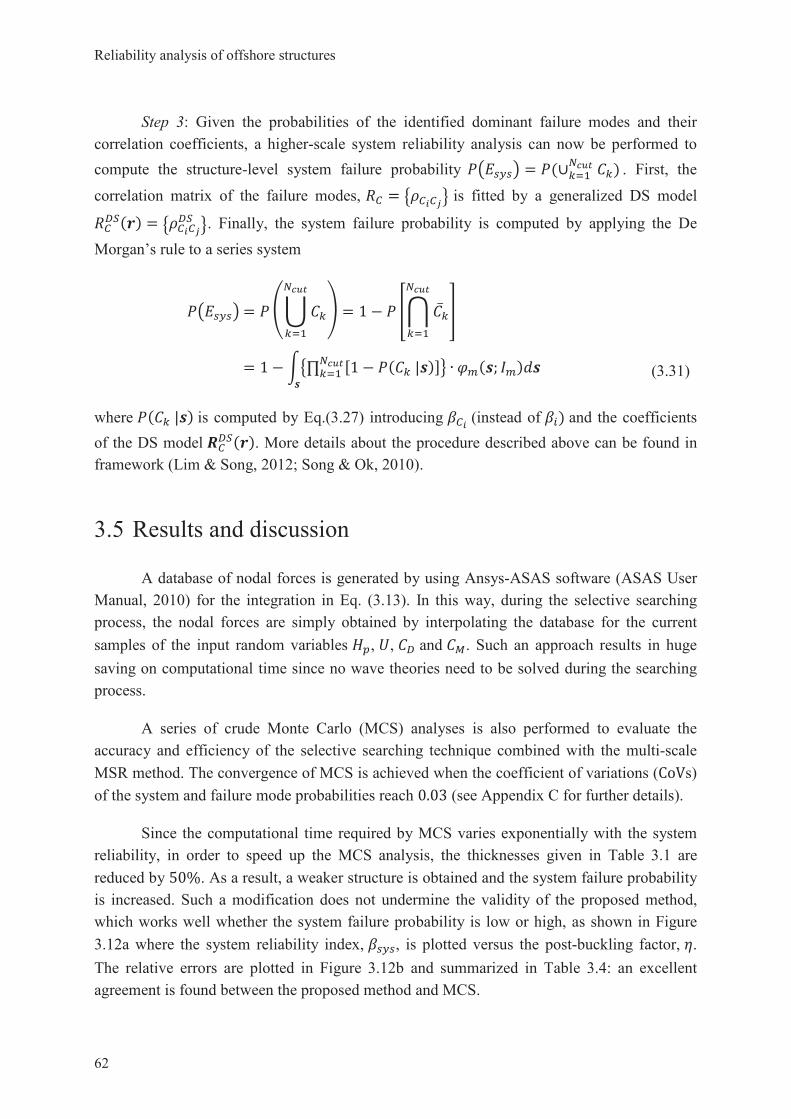
Reliability analysis of offshore structures
62
Step 3: Given the probabilities of the identified dominant failure modes and their
correlation coefficients, a higher-scale system reliability analysis can now be performed to
compute the structure-level system failure probability = ( ) . First, the
correlation matrix of the failure modes, = is fitted by a generalized DS model
( ) = . Finally, the system failure probability is computed by applying the De
Morgan’s rule to a series system
= = 1
= 1 [1 ( | )] ( ; )
(3.31)
where ( | ) is computed by Eq.(3.27) introducing (instead of ) and the coefficients
of the DS model ( ). More details about the procedure described above can be found in
framework (Lim & Song, 2012; Song & Ok, 2010).
3.5 Results and discussion
A database of nodal forces is generated by using Ansys-ASAS software (ASAS User
Manual, 2010) for the integration in Eq. (3.13). In this way, during the selective searching
process, the nodal forces are simply obtained by interpolating the database for the current
samples of the input random variables , , and . Such an approach results in huge
saving on computational time since no wave theories need to be solved during the searching
process.
A series of crude Monte Carlo (MCS) analyses is also performed to evaluate the
accuracy and efficiency of the selective searching technique combined with the multi-scale
MSR method. The convergence of MCS is achieved when the coefficient of variations (CoVs)
of the system and failure mode probabilities reach 0.03 (see Appendix C for further details).
Since the computational time required by MCS varies exponentially with the system
reliability, in order to speed up the MCS analysis, the thicknesses given in Table 3.1 are
reduced by 50%. As a result, a weaker structure is obtained and the system failure probability
is increased. Such a modification does not undermine the validity of the proposed method,
which works well whether the system failure probability is low or high, as shown in Figure
3.12a where the system reliability index, , is plotted versus the post-buckling factor, .
The relative errors are plotted in Figure 3.12b and summarized in Table 3.4: an excellent
agreement is found between the proposed method and MCS.

Chapter 3
63
A further consideration about Figure 3.12 reveals the monotonically increasing trend
of the system reliability index. As far as the post-failure behaviour moves from the brittle
zone (lower ) to the ductile zone (higher ), the redundancy level in the structure increases.
On the other hand, the system failure probability decreases with and this increases the
computational cost of MCS exponentially as shown in Figure 3.13, especially for exceeding
0.5. Below this threshold, the number of iterations (and time) required by MCS is almost
constant due to the fact that a minimum of 500,000 analyses is performed to account for the
transient at the beginning of the convergence process (see Section 2.1.8, Example 2.3). By
contrast, the computational cost of the selective searching technique is not heavily affected by
the system failure probability (or , as shown in Figure 3.13). The number of iterations and
the computational time required by this method are 1-2 orders of magnitude less than those
required by MCS and this gap increases as the system failure probability decreases. It is
important to note that the total time trend for the selective searching technique is not strictly
related to the corresponding number of iterations trend, as in the case of MCS. This is due to
the integrations performed by the MSR solver, whose computational time depends on the
number of failure modes identified during the searching process. The numerical data
corresponding to Figure 3.13 are summarized in Table 3.5.

Reliability analysis of offshore structures
64
Figure 3.12: a) Influence of the post-buckling factor on the system reliability; b) relative
errors between the proposed method (GA-MSR) and MCS.
Table 3.4: Results comparison between the selective searching technique and MCS.
Post-buckling FactorReliability Index error [%]
GA-MSR MCS (CoV = 3%)
0.00 2.1209 2.1218 0.04
0.10 2.1233 2.1219 0.07
0.20 2.1350 2.1264 0.40
0.30 2.1615 2.1303 1.46
0.40 2.2169 2.1853 1.45
0.50 2.3613 2.3461 0.65
0.60 2.5515 2.5771 0.99
0.70 2.7880 2.8088 0.74
0.80 2.9851 3.0156 1.01
0.90 3.3057 3.2445 1.89
1.00 3.3992 3.4182 0.56
0 0.2 0.4 0.6 0.8 12
2.2
2.4
2.6
2.8
3
3.2
3.4
0 0.2 0.4 0.6 0.8 10
0.2
0.4
0.6
0.8
1
1.2
1.4
1.6
1.8
2
GA-MSR
MCS
a) b)

Chapter 3
65
Figure 3.13: Influence of the post-buckling factor on the computational costs of the
selective searching technique and MCS in terms of a) iteration number and b) computational
time.
Table 3.5: Comparison of the computational costs required by the selective searching
technique and MCS.
Post-
buckling
factor
GA-MSR MCS (CoV = 3%)
CPU time [s]
# iterationsCPU time
[s]# iterations
Failure
mode
search
System
reliabilityTotal
0.00 201 166 367 15105 11862 730000
0.10 215 227 442 5542 11628 730000
0.20 65 0.1 65 3113 7959 500000
0.30 89 18 107 4484 8347 500000
0.40 214 950 1164 76190 8077 500000
0.50 256 1301 1557 22881 8054 500000
0.60 198 1117 1315 42256 11743 700000
0.70 345 1623 1968 27526 14462 890000
0.80 418 2536 2955 38669 25015 1530000
0.90 193 1.155 1348 33685 52203 3180000
1.00 461 1327 1788 11025 85145 4890000
0 0.2 0.4 0.6 0.8 110
3
104
105
106
107
0 0.2 0.4 0.6 0.8 110
1
102
103
104
105
GA-MSR
MCS
GA-MSR
MCS
a) b)

Reliability analysis of offshore structures
66
Figure 3.14 illustrates the failure modes identified for = 0.5, and their reliability
indexes are reported in Table 3.6a for comparison with MCS. The failure modes are here
arranged in the decreasing order of their likelihood. The following notation is used: -9
(7,8) means, after element 9 fails in compression and the corresponding stress redistribution
occurs, both elements 7 and 8 fail in tension. It is worthwhile to note the relative error
increases with higher reliability indexes, especially for the last three modes. This is probably
due to nonlinearities in the wave-current loads that occur for high values of the wave height,
. This fact can be explained by means of Figure 3.15, where the horizontal wave-current
force is evaluated at two different locations, a node of the jacket (at the intersection between
elements 15 and 16, see Figure 3.3) and a node of the deck (between elements 24 and 27).
The load is plotted versus the wave height, , while , and are assumed equal to their
mean values. As long as is small, the wave affects the jacket only, and the response is
linear. Conversely, nonlinearities are introduced in the deck nodal load for exceeding
22 m, when the wave reaches the top side of the platform. So far, the results provided by
MSR have been calculated performing FORM method. If SORM is used to calculate the
reliability indexes in Eq. (3.27), a better accuracy of MSR can be achieved for low probability
failure modes, as can be noted in Table 3.6b for the last three modes. However, for small
values of (or equivalently, for low reliability indexes) MSR combined with FORM method
still provides a better approximation, as shown in Table 3.6a for the first three modes.
A similar behaviour is presented in Table 3.7, where the accuracy of MSR employing
FORM and SORM is verified for a post-buckling factor = 0.8. The results provided by
SORM are not always more accurate to those provided by FORM, but, on average, the
relative error of the first is 10% less. The minimal cut set representation of the system failure
event for = 0.8 is illustrated in Figure 3.16.
Figure 3.14: Minimal cut set representation of the system failure event for = 0.5.

Chapter 3
67
Table 3.6: Failure modes and corresponding reliability indexes for = 0.5: a) Results
provided by MSR performing FORM compared to MCS; and b) results provided by MSR
performing SORM compared to MCS.
Reliability Index a)
Failure modes MSR (FORM) MCS (CoV = 3%) Error %
- 2.4227 2.4217 0.04
- 2.4521 2.4577 0.23
- 2.5527 2.5752 0.87
- -13) 3.0402 3.0777 1.22
(-9,-10) 3.4201 3.4923 2.07
(-9,-10,-13) 3.5631 3.6535 2.47
Reliability Index b)
Failure modes MSR (SORM) MCS (CoV = 3%) Error %
- 2.4013 2.4217 0.84
- 2.4321 2.4577 1.04
- 2.5285 2.5752 1.81
- -13) 3.0518 3.0777 0.84
(-9,-10) 3.454 3.4923 1.10
(-9,-10,-13) 3.5974 3.6535 1.54
Figure 3.15: Horizontal component of wave-current load calculated at a) the node between
elements 15-16 (see Figure 3.3) and b) the node between elements 24-27.
14 16 18 20 22 24 26 28 30 32 34
80
100
120
140
160
180
200
220
240
260
14 16 18 20 22 24 26 28 30 32 340
50
100
150
200
250
300
350
400
450
a) b)

Reliability analysis of offshore structures
68
Figure 3.16: Minimal cut set representation of the system failure event for = 0.8.
Table 3.7: Failure modes and corresponding reliability indexes for = 0.8: a) Results
provided by MSR performing FORM compared to MCS; and b) results provided by MSR
performing SORM compared to MCS.
Reliability Index a)
Failure modes MSR (FORM) MCS (CoV = 3%) Error %
- 3.0467 3.1018 1.78
- 3.0798 3.1347 1.75
- 3.1728 3.2397 2.07
- -13) 3.2381 3.3231 2.56
- -13) 3.2460 3.3310 2.55
- -13) 3.2658 3.3493 2.49
(-9,-10) 3.4201 3.4796 1.71
(-9,-10,-13) 3.5631 3.6419 2.16
Reliability Index b)
Failure modes MSR (SORM) MCS (CoV = 3%) Error %
- 3.0374 3.1018 2.08
- 3.0777 3.1347 1.82
- 3.1669 3.2397 2.25
- -13) 3.2516 3.3231 2.15
- -13) 3.2606 3.3310 2.11
- -13) 3.2795 3.3493 2.08
(-9,-10) 3.4494 3.4796 0.87
(-9,-10,-13) 3.5683 3.6419 2.02

Chapter 3
69
3.6 Conclusions
This chapter presents an efficient and accurate method for risk assessment of offshore
structures. First, the problem of a jacket-type platform under an extreme sea state is
considered. The structure is modelled as a truss and uncertainty affects the yield stress of the
members, which are assumed to fail either in tension or compression. Environmental loading
includes current-wave forces, self-weight, buoyancy forces and applied loads, in which the
probability density function of the wave height is fitted by a generalized extreme value
distribution, while the current speed and the drag and mass coefficients are assumed to be
normally distributed. Then, a risk assessment framework recently developed for truss and
frame structures is applied to an offshore structure. The main advantage of the approach is
that the identification process of dominant failure modes is decoupled from the evaluation
process of the probabilities of failure modes and the system event. As a result, the dominant
failure modes of the jacket-type platform can be rapidly identified. For this purpose, a multi-
point parallel search employing a genetic algorithm is used. Finally, the evaluation process is
carried out by a multi-scale Matrix-based System Reliability (MSR) analysis, in which the
statistical dependence among both components and failure modes is fully considered.
The accuracy and the efficiency of the proposed approach are successfully validated
against crude Monte Carlo Simulation (MCS). In particular, the computational time and the
number of iterations are 1-2 orders of magnitude less than those required by MCS. The effect
of the post-buckling factor on structure-level failure probability is also investigated. As far as
the post-failure behaviour moves away from the brittle zone (lower post-buckling factor) to
the ductile zone (higher post-buckling factor) the redundancy level in the structure is
enhanced and accordingly, the system reliability index increases. Moreover, while the
computational time required by MCS varies exponentially with system reliability index, the
time required by the proposed method is insensitive to this value.
Finally, the effect of nonlinearities in the wave-current loads on the accuracy of the
results is analysed. When the wave height exceeds a certain value, even the top side of the
structure (the deck) is involved in the calculation of the wave-current forces. As a
consequence, a sharp nonlinear increase in wave-current forces is typically related to outer
regions of the random variables space (where the wave height is higher). It follows that the
probabilities estimated by MSR performing first-order reliability method (FORM) may be
less accurate for failure modes that are less likely to occur. In some cases, a more accurate
estimation of such failure probabilities can be obtained by coupling MSR with second-order
reliability method (SORM).
In conclusion, the computational efficiency and accuracy arising from the capability to
separate the failure mode identification from the probability evaluation processes first, and to
rationally consider the statistical dependence among failure events then, make the proposed

Reliability analysis of offshore structures
70
approach particularly attractive to the offshore industry. Further research will investigate the
applicability of this method to both design and planning of inspection, maintenance and repair
strategies.

71
4 Simulation of the longitudinal tensile
strength and damage accumulation
in fibre-reinforced composites
In this chapter, system reliability theory is applied to the uncertainty quantification of
the longitudinal tensile strength of fibre-reinforced composites. The damage accumulation
and failure of this class of materials is governed by statistical size effects, which pose a
challenge to use coupon-based experimental data for the design of large structures. In this
respect, a Monte Carlo progressive failure analysis is proposed to evaluate the strength
distributions of hierarchical fibre bundles, which are formed by grouping a predefined number
(coordination number) of smaller-order bundles into a larger-order bundle. The present
approach is firstly validated against a recent analytical model, which has been extensively
validated against experimental results. Based on this model, hierarchical bundles are formed
by grouping sub-bundles two by two (i.e., a coordination number equal to two is used), and
their full strength distributions are derived based on given fibre-strength distribution and
matrix shear-lag near fibre breaks. Furthermore, such a model allows the damage
accumulation into clusters of fibre breaks to be analysed. In addition to providing the same
results of the analytical model, the proposed numerical approach is also applied to higher
coordination numbers, thus extending the analysis to more realistic load-sharing
configurations and making this approach suitable for the stochastic analysis of fibre-
reinforced composites and the associated size effects.
This chapter is organised as follows: Section 4.1 introduces the problem of size effects
on the longitudinal tensile strength of fibre bundles. Then, a brief overview of the reference
analytical model is presented in Section 4.2, providing the basis for the numerical
implementation in Section 4.3. Results of the proposed numerical model are shown in Section
4.4, and pros and cons are discussed in Section 4.5. Finally, the main conclusions are drawn
in Section 4.6.

Simulation of the logitudinal tensile strength and damage accumulation in fibre-reinforced composites
72
4.1 Size effects
UniDirectional (UD) fibre-reinforced polymers (FRPs) are generally composed of
millions of individual fibres all aligned in the same direction. Technical fibres, such as glass-
and carbon-fibres, are characterised by micro-scale diameters ( 4 7 m ), high tensile
stiffness ( 200 600 GPa ), and high tensile strength ( 3 7 GPa ) (Pimenta, 2015).
Nevertheless, they are usually very brittle, and their failure is governed by the statistics of
defects. As a consequence, the fibre strength is a random quantity dependent on the size
(length) of the fibre itself; longer fibres are associated to a higher percentage of defects and,
therefore, to weaker strengths. From a reliability point of view, this is explained by the
Weakest Link Theory (WLT) (Weibull, 1951), which states that chain of elements
withstands an external load only if all its elements survive the resulting stresses. This is
mathematically expressed by Eq. (2.68), which is here rewritten as
= 1 { > 0} (4.1)
where is the remote applied stress, and is the longitudinal tensile strength of the -th
fibre element. Let the random variables be all statistically identical and independent, with
= , , in which the subscript U indicates the uniform loading condition, and r indicates
the reference length of the element. Therefore, Eq. (4.1) becomes
= 1 , > = 1 1 , (4.2)
Analogously to the notation used for the strength variables, the failure probabilities are
denoted by , for the elements (length ) and , for the chain (length = ), so that
Eq. (4.2) can be reformulated as
, ( ) = 1 1 , ( ) (4.3)
This is the expression of the WLT for length scaling of the individual fibre strength
distribution. Figure 4.1 illustrates how the length scaling law operates for different ratios
. For any given distribution , (black curve), the output cumulative distribution
function (CDF) of , shifts to lower strength values if > (red curve); conversely,
higher strength values are associated to shorter fibres, i.e. < (green curve).

Chapter 4
73
Figure 4.1: Size effects on the fibre-strength distributions.
The Weibull distribution (Weibull, 1951) is typically used to model the strength of
brittle materials. In this case, the failure probability of a fibre under uniform stress is
, ( ) = 1 exp (4.4)
where is the fibre length, and m and are respectively the shape (size independent) and
scale (measured at the reference length ) parameters of the distribution. It should be noted
that the Weibull distribution verifies Eq. (4.3), therefore Eq. (4.4) is consistent with the WLT.
At the FRP level, the presence of matrix and the load redistribution among parallel
fibres result in a quasi-brittle failure. Micro-bundle (with 4 7 fibres) strengths have been
measured by Beyerlein and Phoenix (1996) and Kazanci (2004), highlighting significant
deviations from the Weibull model; in particular, some bundles resulted in higher mean
strengths and lower variability than the single fibres. At the macroscopic scale (with
thousands of fibres), Okabe and Takeda (2002) and Scott et al. (2011) observed several
clusters of fibre breaks forming before global failure; moreover, both the mean value and the
variability of strength decrease for larger specimens (Wisnom, 1999). All these observations
are incompatible with the WLT applied directly to the single-fibre level (Bažant, 1999;
Wisnom, 1999).
Hence, several modelling approaches have been suggested for the stochastic analysis
of FRPs (Bažant, 1999; Wisnom, 1999). Fibre Bundle Models (FBMs) (Pradhan, Hansen &
Chakrabarti, 2010) accurately represent the physics involved in longitudinal tensile failure
and the associated size effects. This type of model focuses on calculating the strength
distribution of a bundle of fibres with a given characteristic length, and the WLT is only used
to scale the result for a longer chain of bundles (Curtin, 1991; Harlow & Phoenix, 1978a,b).
0
0.1
0.2
0.3
0.4
0.5
0.6
0.7
0.8
0.9
1
3 4 5 6 7 8 9

Simulation of the logitudinal tensile strength and damage accumulation in fibre-reinforced composites
74
Figure 4.2: Fracture contours within a fibre bundle, at three different
magnification levels (Pimenta et al., 2010).
In general, the complexity of FBMs increases with the number of fibres in the
bundle’s cross-section, and exact solutions are attainable for small bundles only. However,
quasi-fractal fracture surfaces (i.e. fracture surfaces with similar contours at different
magnification levels, see Figure 4.2) have been reported in UD laminas and fibre bundles
(Laffan et al., 2010; Pimenta et al., 2010), providing experimental evidence for a hierarchical
failure process. Consequently, Pimenta and Pinho (2013) recently proposed a hierarchical
scaling law relating the strength distributions of consecutive bundle levels, in which the
number of fibres scales by a power of two (i.e., a coordination number = 2 is used; see
Figure 4.3a).
Figure 4.3: a) First 4 bundle levels with coordination number = 2; b) Fibre arrangements
for different coordination numbers.
Despite this approach allows a fast calculation of bundle strength distributions,
imposing a coordination number equal to 2 results in too high stress concentrations in the
proximity of fibre breaks. In order to improve the model and to investigate the physics at the
500 m 100 m 50 m
a)
b)

Chapter 4
75
base of the damage accumulation and failure processes of UD composites, the hierarchical
approach is here generalised to higher values of (see Figure 4.3b), thus extending the
analysis to more realistic load-sharing configurations (of particular interest is the case of
= 7, which better represents the actual disposition of fibres in the bundle cross-section).
However, the number of possible bundle failure sequences becomes extremely high
for > 2, thus preventing the bundle strength distributions to be evaluated analytically. A
new numerical approach is then proposed, where the failure events are simulated through a
discrete representation of hierarchical bundles, and their distributions are evaluated by means
of a Monte Carlo progressive failure analysis.
4.2 Overview of the hierarchical analytical model for
composite fibre bundles
4.2.1 Hierarchical scaling law for the bundle strengths
As shown in Figure 4.3a, the analytical model (Pimenta & Pinho, 2013) assumes that
hierarchical bundles are formed by pairing two individual fibres (level-[0]) into a level-[1]
bundle, and sequentially grouping two level-[ ] bundles into one level-[ + 1] bundle.
Consider first a level-[1] bundle composed by two level-[0] fibres, and , and
assume the far-field stress progressively increasing until a first break occurs in the middle
of fibre (see Figure 4.4). Based on a perfectly-plastic shear-lag model, the failed fibre
recovers the remote stress within the level- [0] effective recovery length (Pimenta &
Pinho, 2013), i.e.
[ ]( ) = 2
[ ](4.5)
where is the cross-sectional area of a single fibre, is the matrix/interface yield stress in
shear, and [ ] is the perimeter of the level-[0] shear-lag boundary, at which shear stresses
can be transferred. From equilibrium, a linear stress concentration applies to fibre , which
reaches a stress concentration factor = 2 in the proximity of the fibre break ( = 0).
Bundle failure requires fibre to fail nearby the break in fibre , so as to promote
complete yielding of the matrix/interface between the two fibre-breaks (see Figure 4.5).
Therefore, once fibre fails, the level-[1] control region is defined as the region where a
break in fibre would lead to bundle failure, i.e.
[ ]( ) = 2
[ ]( ) (4.6)

Simulation of the logitudinal tensile strength and damage accumulation in fibre-reinforced composites
76
Figure 4.4: A first break occurs in the middle of fibre , the matrix yields plastically, and a
linear stress concentration applies to fibre (Pimenta & Pinho, 2013).
Figure 4.5: Definition of the critical distance between fibre breaks: the bundle fails
if fibre breaks at a distance smaller than /2 = e from the break
in fibre (Pimenta & Pinho, 2013).
Figure 4.6: Definition of the control region and fibre segments in a
level-[1] bundle (Pimenta & Pinho, 2013).

Chapter 4
77
As illustrated in Figure 4.6, the control region is partitioned into 4 segments ( , ,
and ) of equal length [ ]
, and two assumptions are made:
( ) the bundle is represented by a chain of independent control regions (to avoid bundle-
end effects by shifting the first fibre-break to the centre of the control region);
( ) within a control region, each fibre can fail only once (to guarantee simple stress fields
as those presented in Figure 4.5).
Based on the assumptions above, the list of sequences of events leading to bundle
failure is defined as follows:
: failure of segment and unstable failure (with no increase of the far-field stress) of
segment due to stress concentrations;
: failure of segment and stable failure (after incrementing ) of segment due to
stress concentrations;
: failure of segment and stable failure of segment due to independent fibre flaws
(including growth and coalescence of matrix damage between fibre breaks).
Therefore, the total failure probability of the bundle is given by the union of events ,
and , which yields the following expression for the level-[1] bundle survival probability
under uniform stress within the control length [ ]
(see Appendix D):
,
[ ]( ) = ,
[ ]( ) + 2 1 ,
[ ]( ) ,
[ ]( ) ,
[ ]( ) (4.7)
where ,
[ ]and ,
[ ]are the survival probability of a single-fibre segment of length
[ ], and
the subscripts U and K respectively refer to a uniform stress loading ( ) and a linear stress
profile with concentration factor = 2. The level-[1] bundle strength distribution is then
obtained as the complement of the level-[1] bundle survival probability, i.e. ,
[ ]( ) = 1
,
[ ]( ).
Eq. (4.7) relates the strength distribution of the level-[1] bundle to that of a single
fibre, for which a Weibull distribution is used in (Pimenta & Pinho, 2013). Assuming a
hierarchical failure process, Eq. (4.7) is then extended to any bundle level, so that the
following recursive formula is provided:
,
[ ]( ) = ,
[ ]( ) + 2 1 ,
[ ]( ) ,
[ ]( ) ,
[ ]( ) (4.8)
in which the control length and the recovery length scale hierarchically too:
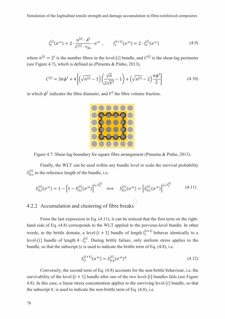
Simulation of the logitudinal tensile strength and damage accumulation in fibre-reinforced composites
78
[ ]( ) = 2
[ ]
[ ] ,
[ ]( ) = 2
[ ]( ) (4.9)
where [ ] = 2 is the number fibres in the level-[ ] bundle, and [ ] is the shear-lag perimeter
(see Figure 4.7), which is defined as (Pimenta & Pinho, 2013),
[ ] = 3 + 4 [ ] 12
1 + [ ] 22
(4.10)
in which indicates the fibre diameter, and the fibre volume fraction.
Figure 4.7: Shear-lag boundary for square fibre arrangement (Pimenta & Pinho, 2013).
Finally, the WLT can be used within any bundle level to scale the survival probability
,
[ ]to the reference length of the bundle, i.e.
,
[ ]( ) = 1 1 ,
[ ]( )
[ ]
,
[ ]( ) = ,
[ ]( )
[ ]
(4.11)
4.2.2 Accumulation and clustering of fibre breaks
From the last expression in Eq. (4.11), it can be noticed that the first term on the right-
hand side of Eq. (4.8) corresponds to the WLT applied to the previous-level bundle. In other
words, in the brittle domain, a level-[ + 1] bundle of length [ ]
behaves identically to a
level-[ ] bundle of length 4[ ]
. During brittle failure, only uniform stress applies to the
bundle, so that the subscript is used to indicate the brittle term of Eq. (4.8), i.e.
[ ]( ) = ,
[ ]( ) (4.12)
Conversely, the second term of Eq. (4.8) accounts for the non-brittle behaviour, i.e. the
survivability of the level-[ + 1] bundle after one of the two level-[ ] bundles fails (see Figure
4.8). In this case, a linear stress concentration applies to the surviving level-[ ] bundle, so that
the subscript is used to indicate the non-brittle term of Eq. (4.8), i.e.

Chapter 4
79
[ ]( ) = 2 1 ,
[ ]( ) ,
[ ]( ) ,
[ ]( ) (4.13)
Eq. (4.13) can then be used to determine the frequency of occurrence of level-[ ]
clusters, which are defined considering every occurrence of a failed level-[ ] bundle with a
surviving level-[ ] neighbour (see Figure 4.8). In particular, the density of level-[ ] clusters in
any bundle of level greater than or equal to [ + 1] is given by (Pimenta, 2014)
[ ]( ) =
[ ]( )
[ ]( )
, [ ]
( ) = [ ] [ ]( ) (4.14)
where [ ]
represents the control volume of the level-[ + 1] bundle.
Figure 4.8: Damaged level-[ + 1] bundle of length [ ]
, in which only one of
the two level-[ ] bundles withstands the external load.
From the definition of clusters given above, the surviving level-[ ] bundle may still
present broken fibres, whose density is denoted by [ ]
. With reference to Figure 4.8, the
following recursive formula is provided
[ ]( ) = [ ] [ ]
( ) +[ ]
( ) (4.15)
in which the first term represents the contribution of the broken level-[ ] bundle (blu area),
and the second term is the contribution of the survived level-[ ] bundle (red area).
The total number of broken level-[ ] clusters and fibre breaks in a level-[ ] bundle of
length can be defined as
[ | ]( ) =
[ ]( )
[ ] , {0, … , 1} (4.16)
[ ]( ) =
[ ]( )
[ ] , where
[ ]= [ ] (4.17)

Simulation of the logitudinal tensile strength and damage accumulation in fibre-reinforced composites
80
Finally, the largest cluster in a level-[ ] bundle is defined as the largest level ,
[ ]
which guaranties a pre-established minimum value of [ | ]
, e.g.
,
[ ]( ) = max {0, … , 1}
[ | ]( ) 0.5 (4.18)
4.3 Numerical implementation
4.3.1 Simulation of failure events in a bundle with 2 fibres
The analytical hierarchical model introduced in the previous section is here
reformulated using a discrete representation of fibres and bundles. Consider first a level-[1]
bundle of length [ ] and coordination number = 2 (i.e. a 2-fibres bundle), in which each
fibre is discretised into a large number of level-[0] elements of equal length [ ]. A value of
strength is then generated for each fibre-element (Figure 4.9a), based on a random sampling
of level-[0] strength distribution. A Weibull distribution is assumed for the individual fibres
(for consistency with Pimenta and Pinho’s (2013) analytical model); being the reference
length at which the Weibull parameters were measured, the distribution used in the model is
then scaled to the element length [ ] by applying the WLT,
, [ ]
[ ]( ) = 1 1 ,
[ ]( )
[ ]
(4.19)
where ,
[ ]and
, [ ]
[ ]denote the Weibull distribution at length and [ ] , respectively.
Finally, the element strengths are generated by inverse transform sampling method (Devroye,
1986), applied to the level-[0] strength distribution, , [ ]
[ ].
Figure 4.9a illustrates a situation where the applied stress overcomes the strength
of elements 6 and 8 of fibre , and of element 15 of fibre , thus leading to local failures
(highlighted in red colour). The corresponding stress field is shown in Figure 4.9b, which
satisfies the equilibrium equation
, + , = 2 (4.20)
where the stresses , and , are evaluated at the centre of the -th element of fibre and
, respectively.

Chapter 4
81
As shown in Figure 4.9b, the resulting stress fields can be more complex than those
assumed in the analytical model (Figure 4.5). This is because the numerical implementation
does not involve assumptions ( ) and ( ), and the recovery regions can be here defined by
superimposition of multiple stress-recovery fields (e.g., recovery region 1 in Figure 4.9b).
Figure 4.9: a) Elements 6 and 8 of fibre and element 15 of fibre fail under the uniform
stress ; b) Resulting stress fields with recovery regions in red
and stress concentrations in green.
However, the proposed implementation preserves the basic sequences of events
leading to bundle failure, i.e. , and defined in Section 4.2.1. This result is achieved by
means of a progressive failure analysis, where the far-field stress is increased starting
from the strength value of the weakest element (at which the first local failure occurs), up to
the termination of the analysis once a global failure of the bundle is detected (see Figure 4.10
- Figure 4.12). Global failures occur when a recovery region in one fibre overlaps at least one
recovery region in the other fibre, so that the equilibrium Eq. (4.20) cannot be satisfied. At
that point, the value of the far-field stress is stored as an outcome of the stochastic level-
[1] bundle strength, , [ ]
[ ]. The corresponding distribution
, [ ]
[ ]is obtained by a Monte
Carlo analysis, repeating the progressive failure analysis ( = 10 ) times, each time
randomly sampling the element strengths from the given individual fibre strength distribution.
1 2 3 4 5 6 7 8 9 10 11 12 13 14 15 16 17 18 19 200
0.5
1
1.5
2x 10
4
1 2 3 4 5 6 7 8 9 10 11 12 13 14 15 16 17 18 19 200
0.5
1
1.5
2x 10
4
1 2 3 4 5 6 7 8 9 10 11 12 13 14 15 16 17 18 19 200
0.5
1
1.5
2x 10
4
1 2 3 4 5 6 7 8 9 10 11 12 13 14 15 16 17 18 19 200
0.5
1
1.5
2x 10
4
2
a) b)
6 8
15
6 8
15

Simulation of the logitudinal tensile strength and damage accumulation in fibre-reinforced composites
82
Figure 4.10: Unstable failure (event ); the level-[1] bundle fails at the first iteration of
the progressive failure analysis when is equal to the strength value of the weakest
element (i.e., element 15 of fibre : after its failure, fibre does not survive the
stress concentrations in elements 15 and 16). Note the different values of
strength and stress in the vertical axes.
Figure 4.11: Stable failure (event ); the bundle fails after three iterations (the last iteration is
highlighted in red colour). After element 6 of fibre fails, fibre survives the stress
concentrations until reaches the strength of element 7 of fibre . Note
the different values of strength and stress in the vertical axes.

Chapter 4
83
Figure 4.12: Stable failure (event ); the bundle fails due to growth and coalescence
of the recovery regions between two previously formed breaks (in element 15 of
fibre and element 8 of fibre ). Note the different values of strength and
stress in the vertical axes.
4.3.2 Simulation of larger bundles and asymptotic analysis of the strength
distribution
The resulting level- [1] strength distribution is subsequently used to sample the
strengths of level-[1] elements in the simulation of a level-[2] bundle (Figure 4.13). As in the
previous level, the WLT is used for length scaling, so that the level-[1] bundle distribution
can be evaluated at the element length [ ]:
, [ ]
[ ]( ) = 1 1
, [ ]
[ ]( )
[ ] [ ]
(4.21)
Figure 4.13: The WLT is applied to scale the bundle distribution from the full level-[1]
bundle length ( [ ]) to the level-[1] element length ( [ ]), so that the level-[1] element
strengths can be sampled for the analysis of the level-[2] bundle.
2
WLT

Simulation of the logitudinal tensile strength and damage accumulation in fibre-reinforced composites
84
However, the accuracy of , [ ]
[ ]is limited by the finite number of Monte Carlo
analyses ( ), as the right tail of , [ ]
[ ]above the (1 1/ ) -th quantile is unavoidably
rounded up to 1. Consequently, the small ratio [ ] [ ] in Eq. (4.21) leads to the complete
loss of a large portion of , [ ]
[ ](segment - in Figure 4.14), making it impossible to sample
values for the element strength , [ ]
[ ].
Figure 4.14: a) The limited number of Monte Carlo analyses rounds up to 1 the right tail of
both the bundle strength (, [ ]
[ ], blue curve) and the element strength (
, [ ]
[ ], black curve)
distributions; the latter is fitted with the asymptotic distribution (lim, [ ]
[ ]( ),
red curve) provided by the WLT applied to the previous level bundle (Eq. (4.23));
b) region from plot a) highlighted.
This problem is circumvented by means of an asymptotic approximation of the bundle
strength distributions. Pimenta and Pinho (2013) proved that if the individual fibre strength
follows a Weibull distribution, then the Right Tail Asymptote (RTA) of any bundle strength
distribution corresponds to the WLT applied to the single-fibre level, i.e.
lim, [ ]
[ ]( ) = 1 1
, [ ]
[ ]( ) (4.22)
where is the number of individual fibres in the level-[ ] bundle (being the coordination
number). Therefore, a level-[ ] bundle behaves asymptotically like an individual fibre (series
system) with length times the bundle length (see Figure 4.15). Moreover, since the Weibull
distribution is scale-invariant, the RTA defined above is still a Weibull distribution.
However, it can be shown that as the bundle size increases (i.e., large and/or large ),
these asymptotes are valid for progressively more reduced tails (Pimenta & Pinho, 2013). A
modification to the asymptotic analysis is then needed, providing asymptotes that are suitable
for the fitting of the bundle strength distributions even at the macroscopic scale.
0.85
0.88
0.91
0.94
0.97
1
6.5 7 7.5 8 8.5 9
a) b)
b)

Chapter 4
85
Figure 4.15: WLT applied to the single-fibre level (case for = = 2).
Since the right tail of any strength distribution falls into the domain of large stresses
, its shape is governed by unstable bundle failure due to stress concentrations (i.e., event
). In other words, the RTA of the level-[ ] bundle is determined by the strength of its
weakest sub-bundle of level [ 1]. Such a consideration is consistent with the WLT applied
to the previous-level bundle, so that the following model of the RTA is here proposed:
lim, [ ]
[ ]( ) = 1 1
, [ ]
[ ]( )
(4.23)
The geometrical interpretation of Eq. (4.23) is illustrated in Figure 4.16, in which the
asymptotic behaviour of a level-[2] bundle is expressed by the series of its sub-bundles of
level [1].
Figure 4.16: WLT applied to the previous-level bundle (case for = = 2).
Eq. (4.23) is used to fit , [ ]
[ ](by letting = 1, and = 2 in this particular case),
which is then defined by the curve - - - (Figure 4.14). Finally, a tolerance is established
for the residual gap - , which can be further reduced by increasing the ratio [ ] [ ] to a
value closer to unity.

Simulation of the logitudinal tensile strength and damage accumulation in fibre-reinforced composites
86
The difference between the two asymptotic models is shown in the Weibull plot of
Figure 4.17, where the Weibull distributions are represented by straight lines. The data
relative to the first 3 levels are taken from the results that will be presented in Section 4.4,
assuming [ ]= 0.1 mm, = 1, 2 and 3.
Figure 4.17: a) Asymptotic analysis of the first 3 levels using the WLT applied to the
single-fibre level (dashed lines) and to the previous-bundle level (dotted lines);
b) region from plot a) highlighted.
-10
-8
-6
-4
-2
0
2
1 1.25 1.5 1.75 2 2.25 2.5
Monte-Carlo
WLT single-fibre level
WLT previous-bundle level
b)
a)
-2.5
-2
-1.5
-1
-0.5
0
1.8 1.9 2 2.1 2.2 2.3
b)

Chapter 4
87
At level [1] (blue curves), the previous-bundle level corresponds to level [0] (i.e., the
single-fibre level), so that both Eq. (4.22) and Eq. (4.23) provide the same RTA (dashed blue
line). As shown in Figure 4.17b, numerical errors affect the last portion of , [ ]
[ ](solid blue
line) before it is rounded up to 1 (point ). As a consequence, the fitting point is anticipated
from to , where is the first point of , [ ]
[ ]such that the vertical segment satisfies
the pre-established tolerance on the residual gap (e.g., 0.03). In this way, the fitted curve - -
- is replaced by the more accurate curve - - - .
This fitting procedure is extended to higher levels (i.e., 2), at which the RTAs
defined by Eq. (4.23) (dotted lines) depart from the Weibull distribution. It should be noted
the distance between and the Weibull asymptote (dashed lines) increases at higher levels,
thereby preventing , [ ]
[ ]to be fitted using Eq. (4.22). Conversely, the fitting point is
progressively anticipated, suggesting full convergence of high level distributions to the WLT
applied to the previous-bundle level. This fact will be proved in Section 4.4 for 5.
4.3.3 Extension of the numerical model to higher coordination numbers
Figure 4.18a illustrates the case of a level-[1] bundle with coordination number = 3,
where local failures affect elements 4 and 15 of fibre , elements 8 and 12 of fibre , and
element 14 of fibre . Figure 4.18b shows the corresponding stress field, which is calculated
assuming the stress concentration to be equally distributed among intact elements. Therefore,
indicating with , the value of stress evaluated at the -th element of the -th fibre it can be
shown that
, =
[ ]
2, if
+ ( 1) min , , , if
(4.24)
where , is the positive distance from the -th element of the -th fibre to the closest broken
element in the recovery region (more than one element can fail within the same recovery
region, e.g. recovery regions 1 and 2 in Figure 4.18b); and , is a logic operator, which is 1
if the -th element of the -th fibre belongs to and 0 otherwise. The first expression of Eq.
(4.24) comes from Eq. (4.5) and defines the linear stress field in the proximity of the fibre
breaks (red stresses in Figure 4.18b). In the second expression of Eq. (4.24), the term inside
square brackets represents the total stress that must be added to in order to guarantee the
equilibrium within the elements of the -th column. This additional stress is then equally
distributed among the intact elements of the -th column, whose number is given by the term
inside round brackets. The second expression of Eq. (4.24) can also be rewritten as

Simulation of the logitudinal tensile strength and damage accumulation in fibre-reinforced composites
88
, = 1 +( 1) min 1,
,
,
= , if (4.25)
where , ( 1) represents the stress concentration factor that applies to the -th element of
the -th fibre. It should be noted that , enters in the definition of , only if , < , i.e.
when the -th element of the -th fibre ( ) belongs to the recovery region . This implies
, =
[ ]
2, if ,
(4.26)
Figure 4.18: a) Elements 4 and 15 of fibre , elements 8 and 12 of fibre , and element 14 of
fibre fail under uniform stress loading ; b) The whole bundle fails due to non-
equilibrium in elements 13 and 14 (dashed areas).
In order to extend the Monte Carlo progressive failure analysis to higher ’s, it is here
assumed that a global bundle failure occurs when all sub-bundles are broken and all recovery
regions overlap in at least one element (e.g., elements = 13 and = 14 in Figure 4.18b).
When this statement is true, the equilibrium cannot be satisfied, i.e.
: , <(4.27)
2
a) b)
154
8 12
14
154
8 12
14

Chapter 4
89
4.3.4 Optimal discretisation of the fibre bundles
The accuracy of the simulated strength distributions strongly depends on the ratios [ ] [ ]. If, on the one hand, a finer discretisation leads to more accurate estimates of the
strength statistics (mean and coefficient of variation), on the other, it entails longer
computation times. Therefore, the optimal values of element and bundle lengths are
determined at each level [ ], so as to use the minimum number of elements which guarantees
both efficiency and convergence of the output strength distribution.
Figure 4.19: Strategy for an optimal discretisation of the fibre bundles.
N Y
N
STOP
Not able to analyse the next level
MONTE CARLO
N
count = 0
MONTE CARLO
Y
MONTE CARLO
N
Y
N
count = 1? count = 1
Y
,
be fitted? of Pf_L with
Y
LEVEL = LEVEL + 1
(increase the bundle level)
N
Y
?
STOP

Simulation of the logitudinal tensile strength and damage accumulation in fibre-reinforced composites
90
The main steps of the optimisation process are illustrated in Figure 4.19 and they can
be summarised as follows.
Step 1: The analysis starts at level = 1 for given values of [ ] and [ ]. These values
are chosen based on the reference length of the individual fibre, e.g. [ ] = 10 and [ ]= [ ] 1000.
Step 2: In the first loop (yellow blocks), the length of the elements is set equal to [ ]
and their number is increased multiplying the bundle length [ ] by 1.5 until convergence of
, [ ]
[ ]. The latter is achieved when the relative error between the last two estimates is lower
than 0.05% for the mean value and 0.5% for the coefficient of variation. The resulting
distribution is stored as the most accurate estimate of the level-[1] bundle strength
distribution, and it is denoted by ,
[ ]
[ ](the subscript “ma” stands for “most accurate”).
Step 3: In the second loop (blue blocks), the bundle length [ ] is decreased by 10%
until the scaled distribution , [ ]
[ ]can be fitted with the RTA defined in Eq. (4.23). However,
since [ ] has been reduced during the last loop, the accuracy of , [ ]
[ ]must be verified with
respect to the most accurate estimate ,
[ ]
[ ]. To this end,
, [ ]
[ ]is scaled to
[ ]for the
comparison with ,
[ ]
[ ]. In this case, a threshold equal to 1% and 2% is chosen for the
relative error on the mean value and the coefficient of variation, respectively. If this
requirement cannot be satisfied, the analysis stops, otherwise the current value of [ ] is
stored as the optimal length for the level-[1] bundle ([ ]
).
Step 4: The last loop (green blocks) searches for the optimal value of the element
length, [ ]
. Here, the initial value [ ] is increased by 50% until the relative error between
the new generated ,
[ ]
[ ]and
,[ ]
[ ]is reduced to 0.05% and 0.5% respectively for the mean
value and the coefficient of variation; the penultimate value of [ ] is then stored as [ ]
.
Step 5: Finally,[ ]
and [ ]
are used to define the initial values of [ ] and [ ] for
the analysis of the level-[2] bundle. This choice is consistent with the evidence that higher
level distributions converge to the WLT applied to the previous-bundle level (Section 4.3.2).
Therefore, the contribution of the stable failure modes (in particular of event , which
includes growth and coalescence of matrix damage between fibre breaks) becomes
progressively less important and always fewer elements (i.e., ratios [ ] [ ] closer to unity)
are then required to properly simulate the distributions of the bundle strengths. The
optimisation process terminates when a pre-established level [ ] is analysed.

Chapter 4
91
4.4 Results
4.4.1 Inputs and outputs
Table 4.1 presents the list of nominal input parameters of the hypothetical material
considered in the original analytical model (Pimenta & Pinho, 2013). The first four
parameters refer to the Weibull distribution for the strength of individual fibres, being the
mean value and CoV the coefficient of variation, while and are respectively the scale
and the shape parameters. Finally, is the matrix/interface yield stress, the fibre
diameter, the fibre volume fraction, and is the reference length for the scale parameter
. The progressive failure analysis is repeated = 10 times during the Monte Carlo
simulation, and the starting values [ ] and [ ] of the optimisation process (Section 4.3.4) are
set equal to [ ] = 1 mm and [ ]= 0.001 mm (i.e., [ ] = 10 and [ ]= [ ] 1000).
Table 4.1: Input parameters for the numerical implementation.
Mechanical properties Geometry
(GPa) (%) (GPa) (MPa) (%) (mm)
4.5 25 4.93 4.54 70 5 60 10
Figure 4.20: Simulated bundle strength distributions from level [1] to level [15],
and comparison with Pimenta and Pinho’s (2013) model.
0.0
0.1
0.2
0.3
0.4
0.5
0.6
0.7
0.8
0.9
1.0
2.5 3.0 3.5 4.0 4.5 5.0 5.5 6.0 6.5 7.0 7.5
CDF
Monte-Carlo
(Pimenta and Pinho, 2013)
Single fibre
15 10 5 2
1

Simulation of the logitudinal tensile strength and damage accumulation in fibre-reinforced composites
92
4.4.2 Comparison between Monte Carlo analysis and the analytical model
Figure 4.20 illustrates the bundle strength distributions for = 2 and a specimen
length of 10 mm . The simulated strengths (solid lines) of the first 15 levels show good
agreement with Pimenta and Pinho’s (2013) model (dashed lines), proving that the numerical
simulation correctly models the same features as the analytical one.
4.4.3 Effects of the coordination number
Figure 4.21 describes the size effects on the statistics of the strength distributions,
where the value of ranges from 2 to 7. Both the mean value and the CoV of the strength
exhibit common behaviours at different ’s: after an initial strengthening and steep reduction
in variability, both the mean value and the variability of tensile strength gradually decrease
with increasing specimen cross-section (the number of fibres in a level-[ ] bundle is
calculated as ). In particular, for all ’s, the magnitude of size effects starts decreasing for
bundle levels higher than 3, as indicated by the upwards curvature of the right tail of the
curves in Figure 4.21a.
As the coordination number increases, the curves in Figure 4.21 shift to higher mean
strengths and lower CoVs. This strengthening effect is mainly due to lower average stress
concentration factors among intact fibres (or sub-bundles) in the proximity of fibre breaks.
For instance, = 2 and = 1.5 are respectively applied for = 2 as shown in Figure 4.9b
and = 3 in Figure 4.18b.
Table 4.2 reports the optimal discretisation resulting from the procedure described in
Section 4.3.4. The ratio [ ] [ ] corresponds to the number of elements that has been used
to simulate the strength distribution of the level-[ ] bundle. As expected, this number
decreases at higher levels [ ]. In particular, the ratio [ ] [ ] approaches unity about level
[5], at which the strength distribution converges to the WLT applied to the previous-bundle
level. This means that the bundle strength distributions are completely defined by Eq. (4.23)
for 5, so that
, [ ]
[ ]( ) 1 1
, [ ]
[ ]( )
[ ] [ ]
, 5 (4.28)
Furthermore, a more detailed analysis of Table 4.2 suggests a faster convergence to
the WLT for larger values of (e.g., the ratios [ ] [ ] for = 4 decrease for increasing
values of ). However, a better understanding of this trend would be achieved increasing the
number of simulations , which strongly influences the variability of the data in Table 4.2.

Chapter 4
93
Figure 4.21: Bundle strength size effects on the mean value (a) and on the CoV (b)
for coordination numbers ranging from 2 to 7, and comparison
with Pimenta and Pinho’s (2013) model.
2.0
2.5
3.0
3.5
4.0
4.5
5.0
5.5
6.0
6.5
1.E+00 1.E+01 1.E+02 1.E+03 1.E+04 1.E+05
Mean strength
Number of fibres in the bundle
(Pimenta and Pinho, 2013)
Monte-Carlo
a)
0
5
10
15
20
25
1.E+00 1.E+01 1.E+02 1.E+03 1.E+04 1.E+05
Number of fibres in the bundle
(Pimenta and Pinho, 2013)
Monte-Carlo
b)

Simulation of the logitudinal tensile strength and damage accumulation in fibre-reinforced composites
94
Table 4.2: Optimal discretisation of fibre bundles and convergence to the WLT
for different values of the coordination number.
=
1 2 3 4 5 6 7 15[ ] 1.5 2.25 2.25 2.25 2.25 2.25 2.25 2.25 2.25[ ] 0.001 0.0114 0.0259 0.0388 0.0577 2.25 2.25 2.25 2.25[ ] [ ] 1500 197 87 58 39 1 1 1 1
=
1 2 3 4 5 6 10[ ] 3.375 3.375 3.375 3.375 3.375 3.375 3.375 3.375
[ ] 0.00764 0.01722 0.02576 0.05921 3.375 3.375 3.375 3.375
[ ] [ ] 442 196 131 57 1 1 1 1
=
1 2 3 4 5 6 7 8[ ] 2.25 2.25 2.25 2.25 2.25 2.25 2.25 2.25
[ ] 0.001001 0.017176 0.025862 0.086538 2.25 2.25 2.25 2.25
[ ] [ ] 2248 131 87 26 1 1 1 1
=
1 2 3 4 5 6 7[ ] 1.575 1.575 1.575 1.575 1.575 1.575 1.575
[ ] 0.001001 0.017120 0.025820 0.131250 0.131250 0.131250 1.575
[ ] [ ] 1573 92 61 12 12 12 1
=
1 2 3 4 5 6[ ] 1.2 1.2 1.2 1.2 1.2 1.2
[ ] 0.001 0.001 0.0076 0.1714 1.2 1.2
[ ] [ ] 1200 1200 158 7 1 1
=
1 2 3 4 5 6[ ] 1.05 1.05 1.575 1.575 3.54375 3.54375
[ ] 0.001 0.002253 0.039375 0.221484 3.54375 3.54375
[ ] [ ] 1050 466 40 7 1 1

Chapter 4
95
4.4.4 Analysis of damage accumulation
Consider first the case of = 2. The damage evolution into clusters of broken fibres is
completely defined by the non-brittle term introduced in Section 4.2.2. This term is
evaluated combining Eq. (4.8) and Eq. (4.13) into the following expression
[ ]( ) = ,
[ ]( )
,
[ ]( ) (4.29)
where the right-hand side is recovered by scaling the simulated distributions (Figure 4.20) to
the control length [ ]
and the recovery length [ ]
.
Figure 4.22: Simulated number of broken level-[ ] clusters in the level-[10] bundle of length
= 10 mm, and comparison with Pimenta and Pinho’s (2013) model.
Figure 4.22 illustrates the total number of broken level-[ ] clusters in the level-[10]
bundle of length = 10 mm. The simulated curves (red lines) show good agreement with
Pimenta and Pinho’s (2013) model, with the exception of Figure 4.22d, where the limited
number of analyses run by Monte Carlo leads to zero occurrences of level-[3] clusters. Fibre
breaks start forming at low applied stresses; as approaches the average strength of the
0
100
200
300
400
500
600
0 1000 2000 3000 4000 5000
0
10
20
30
40
50
0 1000 2000 3000 4000 5000
0
1
2
3
4
5
0 1000 2000 3000 4000 5000
0.0
0.2
0.4
0.6
0.8
0 1000 2000 3000 4000 5000
Monte-Carlo
(Pimenta and Pinho, 2013)
Monte-Carlo
(Pimenta and Pinho, 2013)
Monte-Carlo
(Pimenta and Pinho, 2013)
Monte-Carlo
(Pimenta and Pinho, 2013)
a) b)
c) d)

Simulation of the logitudinal tensile strength and damage accumulation in fibre-reinforced composites
96
bundle (4446 MPa), clusters of broken fibres starts forming and growing, until the largest
cluster triggers catastrophic failure of the entire bundle. These results are consistent with
experimental observations (Scott et al., 2011). Similar trends are reported in Figure 4.23 for
the total number of fibre breaks and the associated density.
Figure 4.23: Simulated number of broken fibres (a) and associated density (b) in
the level-[10] bundle of length = 10 mm, and comparison
with Pimenta and Pinho’s (2013) model.
The total number of fibre breaks in the largest cluster can be estimated as ,[ ]
,
where is the coordination number ( = 2 in this case) and ,
[ ]is defined by Eq. (4.18).
The corresponding curve is shown in Figure 4.24. As expected from Figure 4.22c-d, the
largest cluster level is [2] (i.e, 4 broken fibres) by simulation, and [3] (i.e, 8 broken fibres) by
applying Pimenta and Pinho’s (2013) model.
Figure 4.24: Simulated number of broken fibres in the largest cluster of the level-[10] bundle
of length = 10 mm, and comparison with Pimenta and Pinho’s (2013) model.
0
100
200
300
400
500
600
700
0 1000 2000 3000 4000 5000
0
500
1000
1500
2000
2500
0 1000 2000 3000 4000 5000
Monte-Carlo
(Pimenta and Pinho, 2013)
Monte-Carlo
(Pimenta and Pinho, 2013)
a) b)
0
2
4
6
8
10
0 1000 2000 3000 4000 5000
Monte-Carlo
(Pimenta and Pinho, 2013)

Chapter 4
97
Finally, the analysis of damage accumulation is extended to higher coordination
numbers rewriting the brittle term of Eq. (4.12) as a function of . As stated in Section
4.2.2, in the brittle domain, the level-[ + 1] bundle strength converges to the WLT applied to
the previous-bundle level, so that
[ ]( ) = ,
[ ]( ) = ,
[ ]( ) (4.30)
Therefore, Eq. (4.29) for the non-brittle term can now be generalised as
[ ]( ) = ,
[ ]( )
,
[ ]( ) (4.31)
In Figure 4.25a-b, the density of fibre breaks and the size of the largest cluster are
compared with reference to three bundles with equal length = 10 mm and similar cross-
sectional areas: two bundles are defined by 1204 (= 2 , red line; and 4 , green line) fibres
and one bundle by 1296 (= 6 , blue line) fibres. A further example is illustrated in Figure
4.25c-d considering four bundles, of which two with 256 (= 2 , green line; and 4 , red line)
fibres, one with 243 (= 3 , blue line) fibres, and one with 216 (= 6 , grey line) fibres.
Figure 4.25: Density of fibre breaks and size of the largest cluster in bundles with
equal length = 10 mm and similar cross-sectional areas.
0
500
1000
1500
2000
2500
3000
3500
4000
4500
5000
0 1000 2000 3000 4000 5000 6000
0
1000
2000
3000
4000
5000
6000
0 1000 2000 3000 4000 5000 6000
0
5
10
15
20
25
30
35
40
45
0 1000 2000 3000 4000 5000 6000
0
2
4
6
8
10
12
14
16
18
0 1000 2000 3000 4000 5000 6000
a) b)
c) d)

Simulation of the logitudinal tensile strength and damage accumulation in fibre-reinforced composites
98
Despite the coordination number strongly influences the mean values and the
coefficients of variation of the strength distributions (see Figure 4.21), the initial evolution of
fibre breaks and formation of clusters are almost unaffected by different ’s. Therefore, the
damage accumulation at low far-field stresses weakly depends on stress concentration around
fibre breaks, but it is rather due to the intrinsic variability of the fibre strength.
4.5 Discussion
4.5.1 Limitations of the present model
Computational time and convergence to the exact solution are the key factors to
consider when running Monte Carlo progressive failure analysis. On the one hand, small
ratios [ ] [ ] must be used with low-level bundles (see Figure 4.13), where stable failure
events ( and ) are most likely to occur and need a finer discretisation of the fibres (or
sub-bundles) to be accurately simulated. On the other hand, small ratios [ ] [ ]
compromise the RTA fitting (see Figure 4.14) and lead to large data sets slowing down the
computation. Optimal ratios [ ] [ ] must then be established as in Section 4.3.4 for each
bundle level and for each set of mechanical and geometrical properties of the composite
material.
Figure 4.26: Different load-sharing configurations for a bundle with 4 fibres.
Moreover, in the present numerical implementation, bundles with identical number of
fibres but higher coordination number result in higher mean strengths. As explained in
Section 4.4.3, this is mainly due to lower average stress concentration factors among intact
fibres (or sub-bundles) at higher ’s. Figure 4.26 illustrates the case of a bundle with 4 fibres,
which is modelled both as a bundle of level [2] with = 2 (Figure 4.26a) and as a bundle of
a) b)

Chapter 4
99
level [1] with = 4 (Figure 4.26b). According to Eq. (4.25), a stress concentration factor
= 2 applies in the first case, and = 4 3 in the second case. The lower stress
concentration in the latter case leads to a higher mean value of the bundle strength.
Nevertheless, the analytical sequences of events leading to bundle failure ( , and
) are here collected into only one exhaustive global failure criterion, which is defined by the
inequality in Eq. (4.27). Such a criterion may result in very high peaks in the stress profile as
in the case of fibres and in Figure 4.18b, while, in reality, the matrix would not be able to
transfer stresses so effectively without failing. Therefore, the present numerical approach
leads to and overestimation of the strength for high values of the coordination number , and
this contributes to the strengthening effect observed in Figure 4.21.
4.5.2 Advantages of the present model
The numerical model copes with more complex stress fields (see Figure 4.18b) than
the analytical model (Pimenta & Pinho, 2013) (see Figure 4.5), and there is no need to define
a control region – and, consequently, no need to impose assumptions ( ) and ( ) (see
Section 4.2.1) in the former. Therefore, the good agreement between analytical and numerical
results in Figure 4.20 suggests that the predictions of the analytical model are not affected by
these restrictions on the control region.
The arbitrariness of the stress profiles also allows the present analysis to be easily
generalised to any value of the coordination number . Therefore, the coordination number is
treated as a free parameter, and no modifications are made to the numerical implementation
when dealing with different load-sharing configurations.
Finally, a user-defined input distribution (i.e., not necessarily a Weibull) can be used
for the individual fibre strength. For instance, a bi-modal Weibull strength distribution has
been proposed (Watanabe et al., 2014) to account for the effects of two different flaw
populations in the fibres, one operating at longer gauge lengths and characterised by large
variability, and another operating at shorter gauge lengths and associated with smaller
strength variability. Such distribution could be introduced in the present implementation to
further investigate the stochastic behaviour of fibre-reinforced composites and the related size
effects.

Simulation of the logitudinal tensile strength and damage accumulation in fibre-reinforced composites
100
4.6 Conclusions
A new numerical approach was developed to model size effects on the longitudinal
tensile strength of composite fibre bundles. The method applies a discretisation of hierarchical
bundles by grouping chains of level-[ ] bundles into a level-[ + 1] bundle, and a Monte
Carlo progressive failure analysis evaluates the corresponding strength distribution.
A comparison was carried out with the analytical model developed by Pimenta and
Pinho (2013) for the simple case of coordination number = 2 (i.e., grouping fibres and
bundles 2 by 2); the good agreement of results proved that the numerical approach is able to
model the same features as the analytical one (see Figure 4.20).
Furthermore, the numerical method was generalised to any value of the coordination
number . Of particular interest is the case for = 7, which better represents the actual
disposition of fibres in the bundle cross-section. A series of analyses was then carried out for
ranging from 2 to 7, and a strengthening effect was observed for increasing values of (see
Figure 4.21), which is mainly due to lower average stress concentration factors among intact
fibres in the proximity of fibre breaks.
The proposed method was also employed for the analysis of the damage accumulation
process during progressive failure. Although the coordination number strongly influences
the mean values of the strength distributions, the evolution of clusters of broken fibres is not
significantly affected by different configurations of the bundle cross-sections, but it rather
depends on the intrinsic variability of the individual fibre strength.
Work is still underway to improve the global failure criterion and to validate results
against experimental data available in literature. Concerning the first task, more accurate
estimates of the bundle strength distributions would be achieved by redefining the recovery
length to account for the total number of broken fibres in the bundle. This concept is
illustrated in Figure 4.27, representing a level-[1] bundle with coordination number = 4 and
3 broken fibres ( , and ); stresses are recovered within a recovery length [ ]
(given by
Eq. (4.5)), and a stress concentration factor equal to 4 applies to the intact fibre ( ) due to the
equilibrium. As a result, the stress field slope in fibre exceeds the maximum speed (slope)
at which stresses are recovered in the broken fibres (red dashed lines in Figure 4.27). In
reality, the matrix would not be able to transfer stresses so effectively without failing and,
therefore, the present numerical approach leads to and overestimation of the bundle strengths,
which contributes in part to the strengthening effect mentioned above.

Chapter 4
101
Figure 4.27: Influence of the total number of broken fibres on the recovery length.
In the present numerical implementation, the maximum slope of the stress-recovery
field in the broken fibres is assumed to be dependent only on the geometrical properties of the
fibres (i.e., the cross sectional area, , and the shear-lag perimeter, [ ]) and on the material
properties of the matrix (i.e., the yield stress in shear, ). However, the same limit should
also apply to the stress field in the intact fibre , and this would increase the length of the
recovery region as indicated by the red double arrow in Figure 4.27. It follows that a new
definition of the recovery length is needed based on the stress concentration factor in the
intact fibres (or sub-bundles), which in turn depends on the total number of broken fibres (or
sub-bundles) in the bundle.

Simulation of the logitudinal tensile strength and damage accumulation in fibre-reinforced composites
102

103
5 General conclusions
5.1 Summary of major findings
This thesis developed novel methods for reliability analysis of complex structural
systems with particular focus on the risk assessment of offshore structures and the uncertainty
quantification of composite fibre bundles. The overall failure of both these types of structures
is characterised by a huge number of critical sequences of component failures, thus resulting
in a complex system event. However, accurate and efficient evaluation of the system-level
risk can be achieved retaining only the dominant failure modes, i.e. the critical failure
sequences that are most likely to contribute to global structural collapse. These modes must
be identified with respect to the redistribution of the internal load effects after member
failures, and a system reliability analysis method is needed to account for statistical
dependence among components events as well as among failure modes.
In this regard, the merits of a risk assessment framework recently developed for truss
and frame structures (Kim et al., 2013) have been investigated in the first part of this work
(Chapter 3), in view of its extensive application to the offshore field. To this end, the problem
of a jacket-type platform under an extreme sea state was considered, and the accuracy and the
efficiency of the proposed approach were successfully validated against crude Monte Carlo
Simulation (MCS). In the second part of the thesis (Chapter 4), system reliability theory was
applied to the uncertainty quantification of the longitudinal tensile strength of UniDirectional
(UD) composites. Here, a Monte Carlo progressive failure analysis has been proposed to
model the full strength distributions of fibre bundles of any size, thus allowing experimental
data measured in small coupons to be used for the design of large composite structures. These
studies provided the following major findings:
In Chapter 3, a jacket-type platform was modelled as a truss structure with
members failing either in tension or compression. Sources of uncertainty were considered
both in the material properties (yield stress) and in the environmental loading (current-wave
forces mainly). Using the risk assessment framework developed by Kim et al. (2013), the
dominant failure modes of the jacket-type platform were rapidly identified by means of a
multi-point parallel search employing a genetic algorithm. This searching scheme explores

Conclusions
104
regions of the random variable space that are progressively more distant from the mean of the
input random vector (i.e., the point of the random space corresponding to the expected values
of the yield stresses, the wave height, the current speed, and the drag and mass coefficients of
the tubular members). In this way, multiple dominant failure modes are identified in the
decreasing order of their likelihood so that the searching process can be terminated as the
contributions by newly identified modes become negligible (without missing critical failure
sequences). Then, the evaluation process of the probabilities of failure modes and the system
event is carried out by a multi-scale Matrix-based System Reliability (MSR) analysis, in
which the statistical dependence among both components and failure modes is fully
considered through simple matrix operations. Differently from other existing approaches, the
identification process is here decoupled from the probability evaluation process. This feature
helps avoid component and system reliability analyses to be performed repeatedly during the
search process, which otherwise would be computationally too demanding for large structures
with a high level of redundancy. As a result, the proposed method guarantees an efficient
estimation of the system-level risk; in particular, the number of iterations was found to be 1-2
orders of magnitude less than those required by MCS. In order to test the accuracy of the
method, the effect of the post-buckling factor on structure-level failure probability was also
investigated. As far as the post-failure behaviour moves away from the brittle zone (lower
post-buckling factor) to the ductile zone (higher post-buckling factor) the redundancy level in
the structure is enhanced and accordingly, the system reliability index increases. An excellent
agreement was found between the reliability indexes estimated by the proposed method and
by MCS in the entire domain of the post-buckling factor. Moreover, while the computational
time required by MCS varies exponentially with system reliability index, the time required by
the proposed method is insensitive to this value.
In Chapter 4, a new numerical approach was developed to model size effects
on the stochastic longitudinal tensile strength of composite fibre bundles. The method applies
a discretisation of hierarchical bundles by grouping a predefined number (termed
“coordination number”) of chains of level- [ ] bundles into a level- [ + 1] bundle; the
corresponding strength distribution is then simulated by means of a Monte Carlo progressive
failure analysis. This study extended the capabilities of the analytical model developed by
Pimenta and Pinho (2013), which is limited to the simple case of coordination number = 2
(i.e., bundles are grouped 2 by 2). Despite this model allows a straightforward evaluation of
the bundle strengths, imposing = 2 results in very high stress concentrations in the
proximity of fibre breaks. In order to deal with different load-sharing configurations, the
present approach treats the coordination number as a free parameter. Of particular interest is
the case for = 7, which better represents the actual disposition of fibres in the bundle
cross-section. A series of analyses was then carried out for ranging from 2 to 7, and a
strengthening effect was observed for increasing values of , which can be explained by lower
average stress concentrations among intact fibres in the proximity of fibre breaks. The
proposed method was also employed for the analysis of the damage accumulation process

Chapter 5
105
during progressive failure. Although the coordination number strongly influences the mean
values of the strength distributions, the evolution of clusters of broken fibres is not
significantly affected by different configurations of the bundle cross-sections, but it rather
depends on the intrinsic variability of the individual fibre strength
5.2 Future research topics
In the following, some recommendations for future studies and improvements are
suggested:
Concerning the study in Chapter 3, the computational efficiency and accuracy
arising from the capability to separate the failure mode identification from the probability
evaluation processes first, and to rationally consider the statistical dependence among failure
events then, make the proposed approach particularly attractive to the offshore industry.
Further research will then investigate the applicability of this method to both design and
planning of inspection, maintenance and repair strategies. Performing an inspection implies
the reduction of the uncertainty associated with the knowledge of the system. This fact is
reflected by an increase of the reliability index in the case of in-service inspection as well as
in the case of inspection planning at the design stage. In the first case, the reliability of a
structure subjected to fatigue failure can be updated based on new information obtained
during non-destructive inspections (NDIs). In this context, the proposed reliability method
would provide an efficient tool for assessment of lifetime extension of structures beyond their
original design lives. At the design stage, this method would help estimate the time to first
inspection and the interval between subsequent inspections so that a pre-established reliability
level could be guaranteed.
Concerning the study in Chapter 4, work is still underway to improve the
global failure criterion of the fibre bundles and to validate results against experimental data
available in literature. In the current numerical implementation, the stress field is calculated
assuming the stress concentration to be equally distributed among intact elements in the
proximity of fibre breaks. Such a criterion may result in very high peaks in the stress profile,
while, in reality, the matrix would not be able to transfer stresses so effectively without
failing. Therefore, the present numerical approach leads to and overestimation of the mean
values of the bundle strength distributions, and developing a new global failure criterion
would increase the accuracy of the results.

Conclusions
106

107
References
API RP2A-LRFD. (1993). Recommended Practice for Planning and Constructing Fixed
Offshore Platforms, Load and Resistance Factor. (1st ed.).
Ambartzumian, R., Der Kiureghian, A., Ohanian, V., & Sukiasian, H. (1998). Multinormal
probability by sequential conditioned importance sampling: theory and application.
Probabilistic Engineering Mechanics, 13(4), 299–308.
Arnold, B. C., Balakrishnan, N., & Nagaraja, H. N. (1992). A First Course in Order Statistics.
New York: John Wiley.
ASAS User Manual. (2010). Version 13.0. ANSYS, Inc. Southpointe 275 Technology Drive
Canonsburg, PA 15317: http://www.ansys.com.
Ayala-Uraga, E., & Moan, T. (2002). System reliability issues of offshore structures
considering fatigue failure and updating based on inspection. 1st International
ASRANet Colloquium. 8-10 July, 2002, Glasgow, Scotland.
Bažant, Z. P. (1999). Size effect on structural strength: a review. Archive of Applied
Mechanics, 69, 703-725.
Beyerlein, I. J., & Phoenix, S. L. (1996). Statistics for the strength and size effects of
microcomposites with four carbon fibres in epoxy resin. Composites Science and
Technology, 56, 75-92.
Bjerager, P. (1991). Methods for structural reliability computations . In F. Casciati, & J. B.
Roberts, Reliability problems: general principles and applications in mechanics of
solids and structures (pp. 89-136). Springer-Verlag Wien.
Boccotti, P. (2000). Wave mechanics for ocean engineering. Elsevier Oceanography Series.
Bomel Ltd. (2002). System-based calibration of north-west European Annex Environmental
Load Factors to ISO Fixed Structures Code 19902. Report No. C925\04\016R, Rev B.
Boole, G. (1854). Laws of thought. American Reprint of 1854 ed., Dover.
Bourinet, J.-M. (2010). FERUM 4.1 User’s Guide. IFMA.
Bourinet, J.-M., Mattrand, C., & Dubourg, V. (2009). A review of recent features and
improvements added to FERUM software. Proc. of the 10th International Conference
on Structural Safety and Reliability (ICOSSAR’09). Osaka, Japan.
Boyle, P., Broadie, M., & Glasserman, P. (1997). Monte Carlo methods for security pricing.
Journal of economic dynamics and control, 21(8), 1267-1321.
Breitung, K. (1984). Asymptotic approximations for multinormal integrals. Journal of
Engineering Mechanics, 110(3), 357-66.
Chakrabarti, S. K. (2005). Hanbook of offshore engineering. Elsevier.
Cornell, C. A. (1967). Bounds on the reliability of structural systems. Journal of structural
division, ASCE, 93, ST1, 171-200.
Curtin, W. A. (1991). Theory of mechanical properties of ceramic-matrix composites. Journal
of the American Ceramics Society, 74, 2837-2845.

108
Curtin, W. A. (1999). Stochastic damage evolution and failure in fiber-reinforced composites.
Advances in Applied Mechanics, 36, 163-253.
Dean, R. G. (1974). Evolution and development of water wave theories for engineering
application, Vol. I and II. Fort Belvair, VA: Special Report No. 1, Coastal
Engineering Research Center U.S. Army.
Der Kiureghian, A. (2005). First- and second-order reliability methods. In Engineering design
reliability handbook. Boca Raton, FL: CRC Press.
Der Kiureghian, A., & Song, J. (2008). Multi-scale reliability analysis and updating of
complex systems by use of linear programming. Reliability Engineering and System
Safety, 93(2), 288-97.
Der Kiureghian, A., Lin, H.-Z., & Hwang, S.-L. (1987). Second-order reliability
approximations. Journal of Engineering Mechanics, 113(8), 1208-25.
Devroye, L. (1986). Non-Uniform Random Variate Generation. NY: Springer-Verlag.
Ditlevsen, O. (1979). Narrow reliability bounds for structural systems. Journal of Structural
Mechanics, 7(4), 453–472.
Ditlevsen, O., & Madsen, H. O. (2007). Structural Reliability Methods. Lyngby, Denmark:
Technical University of Denmark.
Du, X. (2015). Probabilistic Engineering Design, Lecture notes. Missoury University of
Science and Technology: http://web.mst.edu/~dux/repository/me360/me360.html.
Dunnet, C. W., & Sobel, M. (1955). Approximations to the probability integral and certain
percentage points of a multivariate analogue of Student’s t-distribution. Biometrika,
42, 258–60.
Embrechts, P., Klüppelberg, C., & Mikosch, T. (1997). Modelling Extremal Events for
Insurance and Finance. New York: Springer.
Feng, Y. (1989). A method for computing structural system reliability with high accuracy.
Computers & Structures, 33(1), 1-5.
Fishman, G. S. (1995). Monte carlo: Concepts, algorithms, and applications. N.Y., USA:
Springer-Verlag.
Frangopol, D. M., & Maute, K. (2003). Life-cycle reliability-based optimization of civil and
aerospace structures. Computers and Structures, 81, 397-410.
Genz, A. (1992). Numerical computation of multivariate normal probabilities. Journal of
Computational and Graphical Statistics, 1, 141-150.
Gharaibeh, E. S., Frangopol, D. M., & Onoufriou, T. (2002). Reliability-based importance
assessment of structural members with applications to complex structures. Computers
and Structures, 80, 1113-1131.
Goldberg, G. E. (1989). Genetic algorithms in search, optimization and machine learning.
Reading, MA: Addison-Wesley.
Goodstein, R. L. (2007). Boolean Algebra. Mineola, New York: Dover Publications, Inc.
Guenard, Y. F. (1984). Application of System Reliability Analysis to Offshore Structures.
Stanford, CA: Report No. 71: John Blume Earthq. Engng. Center, Stanford University.

109
Haldar, A. (2006). Recent Developments in Reliability-based Civil Engineering. Singapore:
World Scientific Publishing Company.
Haldar, M., & Mahadevan, S. (2000). Probability, Reliability, and Statistical Methods in
Engineering Design. John Wiley.
Harlow, D. G., & Phoenix, S. L. (1978a). The chain-of-bundles probability model for the
strength of fibrous materials. I: Analysis and conjectures. Journal of Composite
Materials, 12, 195-214.
Harlow, D. G., & Phoenix, S. L. (1978b). The chain-of-bundles probability model for the
strength of fibrous materials. II: A numerical study of convergence. Journal of
Composite Materials, 12, 314-334.
Hasofer, A. M., & Lind, N. C. (1974). Exact and invariant second-moment code format. J.
Engng. Mech. Div. ASCE, 100(EM1), 111-121.
Hohenbichler, M., & Rackwitz, R. (1983). First-order concepts in system reliability.
Structural Safety, 1(3), 177-188.
Hohenbichler, M., & Rackwitz, R. (1988). Improvement of second-order reliability estimates
by importance sampling. Journal of Engineering Mechanics, ASCE, 114(12), 2195-
2199.
Hunter, D. (1976). An upper bound for the probability of a union. Journal of Applied
Probability, 13, 597–603.
Kang, W. H., Lee, Y. J., Song, J., & Gencturk, B. (2012). Further development of matrix-
based system reliability method and applications to structural systems. Structure and
Infrastructure Engineering: Maintenance, Management, Life-cycle Design and
Performance, 8(5), 441–57.
Kang, W.-H., Song, J., & Gardoni, P. (2008). Matrix-based system reliability method and
applications to bridge networks. Reliability Engineering & System Safety, 93, 1584-
1593.
Karamchandani, A. (1987). Structural system reliability analysis methods. Report no. 83.
Department of Civil Engineering, Stanford University.
Karamchandani, A., Dalane, J. I., & Bjerager, P. (1992). Systems reliability approach to
fatigue of structures. Journal of Structural Engineering, 118(3), 684-700.
Kazanci, M. (2004). Carbon fiber reinforced microcomposites in two different epoxies.
Polymer Testing, 23, 747-753.
Kim, D.-S., Ok, S.-Y., Song, J., & Koh, H.-M. (2013). System reliability analysis using
dominant failure modes identified by selective searching technique. Reliability
Engineering and System Safety, 119, 316-331.
Kotz, S., & Nadarajah, S. (2000). Extreme Value Distributions: Theory and Applications.
London: Imperial College Press.
Kounias, E. G. (1968). Bounds for the probability of a union, with applications. The Annals of
Mathematical Statistics, 39(6), 2154–2158.
Kurtz, N., Song, J., Kim, D.-S., & Ok, S.-Y. (2010). Multi-scale system reliability analysis of
bridge structures using dominant failure modes identified by selective searching

110
technique. The Fifth International Conference on Bridge Maintenance, Safety and
Management (IABMAS2010). 2010, July 11-15, Philadelphia, PA.
Laffan, M. J., Pinho, S. T., Robinson, P., & Iannucci, L. (2010). Measurement of the in situ
ply fracture toughness associated with mode I fibre tensile failure in FRP. Part II: Size
and lay-up effects. Composites Science and Technology, 70, 614-621.
Law, A. M., & Kelton, W. D. (2000). Simulation modeling & analysis (3rd ed.). N.Y., USA:
McGraw-Hill, Inc.
Lee, Y. J., & Song, J. (2011). Risk analysis of fatigue-induced sequential failures by branch-
and-bound method employing system reliability bounds (B3 method). ASCE Journal
of Engineering Mechanics, 137(12), 807–21.
Lee, Y. J., & Song, J. (2012). Finite-element-based system reliability analysis of fatigue-
induced sequential failures. Reliability Engineering & System Safety, 108, 131–41.
Lee, Y.-J., Song, J., Gardoni, P., & Lim, H.-W. (2011). Post-hazard flow capacity of bridge
transportation network considering structural deterioration of bridges. Structure and
Infrastructure Engineering: Maintenance, Management, Life-cycle Design and
Performance, 7(7), 509-521.
Lim, H.-W., & Song, J. (2012). Efficient risk assessment of lifeline networks under spatially
correlated ground motions using selective recursive decomposition algorithm.
Earthquake Engineering and Structural Dynamics, 41(13), 1861-1882.
Lin, Y. K. (1967). Probabilistic theory of structural dynamics. New York: McGraw-Hill Inc.
Liu, P.-L., & Der Kiureghian, A. (1986a). Multivariate distribution models with prescribed
marginals and covariances. Probabilistic Engineering Mechanics, 1(2), 105-112.
Liu, P.-L., & Der Kiureghian, A. (1986b). Optimization algorithms for structural reliability
analysis. Report UCB/SESM 86/09. Berkeley: Department of civil engineering,
University of California.
Liu, P.-L., & Der Kiureghian, A. (1992). Optimization algorithms for structural reliability.
Structural Safety, 9, 161–177.
Liu, P.-L., Lin, H.-Z., & Der Kiureghian, A. (1989). CalREL User Manual. Report No.
UCB/SEMM-89/18. Berkeley, CA: Department of Civil and Environmental
Engineering, University of California.
Lutes, L. D., & Sarkani, S. (2004). Random Vibrations: Analysis Of Structural And
Mechanical Systems. Burlington MA: Elsevier Butterworth-Heinemann.
McKay, N. J., Beckman, R., & Conover, W. J. (1979). A comparison of three methods for
selecting value of input variables in the analysis of output from a computer code.
Technometrics, 21, 239–45.
Moan, T. (1994). Reliability and Risk Analysis for Design and Operations Planning of
Offshore Structures. Proc. 6th ICOSSAR, Structural Safety and Reliability, (pp. 21-
43.). Balkema, Rotterdam.
Moan, T. (2005). Safety of offshore structures. Center for Offshore Research and Engineering
CORE, Report 2005-04.

111
Murotsu, Y., Okada, H., Taguchi, K., Grimmelt, M., & Yonezawa, M. (1984). Automatic
generation of stochastically dominant failure modes of frame structures. Structural
Safety, 2, 17–25.
Nguyen, T. H., Song, J., & Paulino, G. H. (2010). Single-loop system reliability-based design
optimization using matrix-based system reliability method: theory and applications.
Journal of Mechanical Design, ASME., 132, 011005-1~11.
Nguyen, T. H., Song, J., & Paulino, G. H. (2011). Single-loop system reliability-based
topology optimization considering statistical dependence between limit states.
Structural and Multidisciplinary Optimization, 44(5), 593-611.
Okabe, T., & Takeda, N. (2002). Size effect on tensile strength of unidirectional
CFRPcomposites - experiment and simulation. Composites Science and Technology,
62, 2053-2064.
Pandey, M. D. (1998). An effective approximation to evaluate multinormal integrals.
Structural Safety, 20, 51-67.
Park, S. Y. (2001). A new methodology for the rapid calculation of system reliability of
complex structures. Architectural Research, 3(1), 71-80.
Pimenta, S. (2014). Hierarchical scaling law for the strength, deformation and damage
accumulation in unidirectional fibre-reinforced composites under tension -
contribution to the Tensile Failure Exercise. Department of Mechanical Engineering,
Imperial College London, UK.
Pimenta, S. (2015). Chapter 25: Fibre failure modelling. In Numerical Modelling of Failure in
Advanced Composite Materials. Elsevier Science and Technology.
Pimenta, S., & Pinho, S. (2013). Hierarchical scaling law for the strength of composite fibre
bundles. Journal of the Mechanics and Physics of Solids, 61, 1337-1356.
Pimenta, S., Pinho, S. T., Robinson, P., Wong, K. H., & Pickering, S. J. (2010). Mechanical
analysis and toughening mechanisms of a multiphase recycled CFRP. Composites
Science and Technology, 70, 1713-1725.
Polak, E. (1997). Optimization. Algorithms and Consistent Approximations (Vol. 124 of
Applied Mathematical Sciences). New York, NY: Springer Verlag.
Powell, M. J. (1969). A method for nonlinear constraints in minimization problems. New
York: Academic Press.
Pradhan, S., Hansen, A., & Chakrabarti, B. K. (2010). Failure processes in elastic fiber
bundles. Reviews of Modern Physics, 82, 499-555.
Rackwitz, R., & Fiessler, B. (1978). Structural reliability under combined load sequences.
Computers and Structures, 9, 489{494.
Rice, J. (2007). Mathematical Statistics and Data Analysis (3rd ed.). Duxbury Press.
Rosenblatt, M. (1952). Remarks on a Multivariate Transformation. Annals of Mathematical
Statistic, 23, 470-472.
Scott, A. E., Mavrogordato, M., Wright, P., Sinclair, I., & Spearing, S. M. (2011). Is situ fibre
fracture measurement in carbon-epoxy laminates using high resolution computed
tomography. Composites Science and Technology, 71, 1471-1477.

112
Sheldon, M. R. (2007). §2.4 Expectation of a random variable. In Introduction to probability
models (9th ed., pp. 38-47). Academic Press.
Song, J., & Der Kiureghian, A. (2003). Bounds on System Reliability by Linear
Programming. Journal of Engineering Mechanics, 129(6), 627–636.
Song, J., & Kang, W. H. (2009). System reliability and sensitivity under statistical
dependence by matrix-based system reliability method. Structural Safety, 31(2), 148–
56.
Song, J., & Kang, W.-H. (2007). Matrix-based system reliability method and applications to
structural systems. Proc. 18th Engineering Mechanics Division Conference of ASCE.
June 3-6, Blacksburg, VA.
Song, J., & Ok, S.-Y. (2010). Multi-scale system reliability analysis of lifeline networks under
earthquake hazards. Earthquake Engineering and Structural Dynamics, 39(3), 259–79.
Srividya, A., & Ranganathan, R. (1992). Automatic generation of stochastically dominant
failure modes in frame structures for reliability studies. Reliability Engineering and
System Safety, 37, 15-23.
Tang, L. K., & Melchers, R. E. (1987). Improved approximation for multinormal integral.
Structural Safety, 4, 81–93.
Thoft-Christensen, P. (1998). On industrial application of structural reliability theory. Proc.
IFIP 98-WG7.5. May 11-13, Krakow, Poland.
Thoft-Christensen, P., & Murotsu, Y. (1986). Application of structural systems reliability
theory. Berlin: Springer-Verlag.
Tvedt, L. (1983). Two second-order approximations to the failure probability. Oslo: Veritas
Rep. RDIV/20-004083, Det norske Veritas.
Tvedt, L. (1988). Second-order reliability by an exact integral. Proc. 2nd IFIP Working Conf.
on Reliability and Optimization on Structural Systems (pp. 377–384). New York:
Springer.
Tvedt, L. (1990). Distribution of quadratic forms in the normal space - application to
structural reliability. Journal of Engineering Mechanics, ASCE, 116(6), 1183–1197.
Watanabe, J., Tanakaa, F., Okudaa, H., & Okabe, T. (2014). Tensile strength distribution of
carbon fibers at short gauge lengths. Advanced Composite Materials, 23(5-6), 535-
550.
WAVE User Manual. (2010). Version 13.0. ANSYS, Inc. Southpointe 275 Technology Drive
Canonsburg, PA 15317: http://www.ansys.com.
Weibull, G. W. (1951). A statistical distribution function of wide applicability. Journal of
Applied Mathematics, 293-297.
Wisnom, M. R. (1999). Size effects in the testing of fibre-composite materials. Composites
Science and Technology, 59, 1937-1957.
Wu, Y.-L., & Moan, T. (1989). A Structural System Reliability Analysis of Jacket using an
Improved Truss Model. Proc. 5th ICOSSAR (pp. 887-894). San Francisco, New York:
ASCE.

113
Yuan, X.-X., & Pandey, M. D. (2006). Analysis of approximations for multinormal
integration in system reliability computation. Structural Safety, 28, 361-377.
Zhang, Y. C. (1993). High-order reliability bounds for series systems and application to
structural systems. Computers & Structures, 46(2), 381-386.
Zhang, Y., & Der Kiureghian, A. (1997). Finite elements reliability methods for inelastic
structures. Report UCB/SEMM - 97/05. Berkeley: Department of civil and
environmental engineering, University of California.
Zwillinger, D., & Kokoska, S. (2000). Standard Probability and Statistics Tables and
Formulae. CRC Press.

114

115
Appendix A:
Regular wave theories
The integration of Morison’s formula in Eq. (3.13) requires the evaluation of the wave
particle velocity, , for which a stream function theory of the 5-th order (Dean, 1974) is
implemented using Ansys-ASASTM
software (ASAS User Manual, 2010). This theory has
been developed for regular (periodic) waves, whose kinematics is completely defined by three
parameters: the wave height, , the wave period, , and the water depth, .
The simplest form of regular wave theory is the linear wave theory (or Airy theory), in
which the wave profile is described in terms of a sine function (see Figure A.1),
( , ) = sin( ) (A.1)
where the three constants , and respectively indicate the amplitude of the wave ( =
/2), the (time) frequency and the wave number (spatial frequency). Eq. (A.1) suggests that
the constant wave profile moves in the horizontal direction with a velocity
= =2
2= (A.2)
being the wave length and the wave period. Furthermore, a dispersion relationship relates
the wave frequency to the wave number ,
= tanh( )
=2
tanh2
(A.3)
where is the gravitational acceleration. Therefore, Eq. (A.3) provides a recursive approach
to the determination of the wave length given the wave period and the water depth (at
the first iteration, tanh can be set equal to 1). Once (and ) is determined, the wave speed
is calculated from Eq. (A.2). Then, the wave particle velocity field ( , ) is recovered from
Airy theory as a linear function of the wave height (Chakrabarti, 2005),
=2
cosh ( + )
cosh( )cos ( ) (A.4)
=2
sinh ( + )
( )sin ( ) (A.5)
where the coordinate system ( , ) is fixed at the still water level (SWL) as illustrated in
Figure A.1.

Regular wave theories
116
Figure A.1: 2D wave motion over flat bottom.
It should be noted that the vertical component is null at the sea bed ( = ) for all
depths in order to satisfy the bottom boundary conditions. Conversely, the value of at the
bottom depends on the ratio / , and it becomes negligible in deep water ( / > 1/2).
Furthermore, the expressions in Eqs. (A.4) and (A.5) are orthogonal to each other so that
when the value of is maximum, the vertical component is null and vice versa. As a
consequence, in the linear theory, the motion of water particles is described by elliptical
closed paths (see Figure A.1). However, net mass transport is generally associated to waves in
the ocean, thus indicating open orbital paths. Such a motion is accounted for by the present
guidelines as an additional current (e.g. 0.2 knots by API guidelines).
Higher-order theories have been developed to deal with deep-water high waves, which
result in wave profiles with steeper crests and shallower troughs. In Chapter 3, a regular
stream function theory is implemented (Dean, 1974). Here, the velocity field is defined by the
stream function ( , , ), i.e. a scalar quantity defined as
( , , )= ,
( , , )= (A.6)
The dependence of on time is circumvented in the stream function theory by expanding
in a series form in a moving coordinate system, i.e.
( , ) = ( ) + ( ) sinh( ) cos( ) (A.7)
where is speed of moving system (the same as the wave velocity), the current velocity (in
this formulation, is negative for opposing current), and the upper limit of the summation

Appendix A
117
determines the order of the theory. In order to select the appropriate order of the theory, the
plot in Figure A.2 needs to be consulted.
Figure A.2: The range of validity of various wave theories (WAVE User Manual, 2010).
With reference to Section 3.2, the dimensionless ratios / and / in Figure
A.2 are calculated using the significant wave height, = 10 m, the peak period, = 14 s,
and the water depth, = 43 m. The resulting point (0.023,0.005) is highlighted in red colour
and lies close to the region of the stream function theory of the 5-th order. Such a theory is
then selected for the purposes of this work.
5

Regular wave theories
118

119
Appendix B:
Dunnett-Sobel class correlation model
The matrix-based procedure described in Chapter 3 (see Eq. 3.25) can be used even in
the case CSRVs are not explicitly identified. One way to identify such implicit common effect
is provided by Dunnett-Sobel (DS) class correlation model (Dunnet & Sobel, 1955). Suppose
= ( , … , ) is a vector of DS class standard normal random variables. This means the
correlation coefficient between and is defined by = for and = 1 .
Then, ’s can be represented by ( + 1) independent random variables:
= 1 + (B.1)
where and , = 1, … , are independent standard normal random variables. In this way,
all the common source effect is implicitly allocated in the random variable S.
When the difference between the actual correlation matrix and the DS-fitted
correlation matrix causes significant errors in the system reliability estimate, one can
generalise the DS model by adding more CSRVs (Song & Kang, 2009). If CSRVs , =
1, … , are used for accuracy, ’s are represented as
= 1 + (B.2)
The correlation coefficients of this generalised DS model are determined by =
, where ’s are the generalised DS model coefficients that describe the
contribution of the CSVR into . The best fit to minimise the error of the DS model
correlation coefficients is obtained by solving the following nonlinear constrained
optimization problem (Powell, 1969)
min ( )
s. t. 1 > 0,
1 < < 1, ,
(B.3)
where denotes the set of , = 1, … , and = 1, … , ; and are respectively the
original correlation matrix and the DS correlation matrix; and denotes the Euclidean norm
of the matrix.

Dunnett-Sobel class correlation model
120
To illustrate the DS fitting procedure, consider a random vector defined by 4
standard normal variables , = 1, … ,4 with an arbitrary correlation matrix, e.g.
= =
1 0.9
0.9 1
0.8 0.6
0.7 0.5
0.8 0.7
0.6 0.5
1 0.4
0.4 1
(B.4)
If one CSRV is used ( = 1), the optimisation problem in Eq. (B.3) leads to
= =
1.0000
0.8558
0.7364
0.6254
(B.5)
= =
1.0000 0.8558
0.8558 0.7324
0.7364 0.6302
0.6254 0.5352
0.7364 0.6254
0.6302 0.5352
0.5422 0.4605
0.4605 0.3911
(B.6)
The coefficients in Eq. (B.6) are pretty far from the original values in Eq. (B.4) and the
objective function is ( ) = 0.6354. A better accuracy can be achieved using two
CSRVs ( = 2):
= =
0.8846 0.4664
0.7891 0.3271
0.3983 0.9172
0.6400 0.1663
(B.7)
= =
1.0000 0.8506
0.8506 0.7296
0.7802 0.6144
0.6437 0.5594
0.7802 0.6437
0.6144 0.5594
1.0000 0.4075
0.4075 0.4372
(B.8)
that implies ( ) = 0.5781. The error can be further reduced using three CSRVs
( = 3):
= =
0.6736 0.4732 0.5678
0.6882 0.6903 0.1934
0.8081 +0.0817 0.5183
0.0233 0.4742 0.8101
(B.9)

Appendix B
121
= =
1.0000 0.9000
0.9000 0.9875
0.8000 0.6000
0.7000 0.5000
0.8000 0.7000
0.6000 0.5000
0.9284 0.4000
0.4000 0.8817
(B.10)
This matrix is very close to the original correlation matrix in Eq. (B.4) and the objective
function has been reduced to ( ) = 0.1183.
By substituting the coefficients in Eq. (B.9) into the generalised DS model in Eq.
(B.2), the standard normal random vector can be rewritten as
=
0.0000
0.1116
0.2677
0.3440
+
0.6736 0.4732 0.5678
0.6882 0.6903 0.1934
0.8081 +0.0817 0.5183
0.0233 0.4742 0.8101
(B.11)
If a system event is defined as a function of , all the common source effect is
stored in the independent standard normal variables , and . Therefore, from the total
probability theorem, it follows
= | , , ( , , ; ) (B.12)
where the trivariate normal distribution with zero mean and 3 × 3 identity correlation
matrix .

Dunnett-Sobel class correlation model
122

123
Appendix C:
System reliability analysis using Monte Carlo
In Chapter 3, the accuracy of the matrix-based system reliability (MSR) method is
validated against crude Monte Carlo analysis. The simulative procedure is here illustrated
through the case study of the bicomponent series system shown in Figure C.1.
Figure C.1: Series systems consisting of two structural components.
Let the yield strengths and be correlated normal variables ( = =
100 MPa, = = 10 MPa, , = 0.5), the external force be an independent normal
variable ( = 5000 N, = 500 N), and the cross sectional areas and be respectively
equal to 80 and 70 mm . Finally, the following system event is considered
= = ( 0) ( 0)
( , ) = , = 1,2 (C.1)
Following the Monte Carlo procedure presented in Section 2.1.8, is estimated
by the empirical average of the indicator function ( , , ), which is equal to 1 if the
outcome ( , , ) of the random vector ( , , ) belongs to the failure domain, and 0
otherwise. In other words, ( , , ) is equal to 1 if any of the following events is verified:
= only the first component fails
= only the second component fails
= both the components fail
(C.2)
The union of the three basic events above is represented by the shaded area in Figure C.2, and
it is equivalent to the system event defined in Eq. (C.1), i.e. = .
, ,

System reliability analysis using Monte Carlo
124
Figure C.2: Sample space for the bicomponent system in Figure C.1.
After running = 6 10 analyses (the simulation terminates when CoV = 0.05), the
following frequencies are obtained by crude MCS,
( ) = 247 = 4.1167 10
( ) = 5819 = 9.6983 10
( ) = 172 = 2.8667 10
(C.3)
Therefore,
= ( ) = ( ) + ( ) + ( )
= (247 + 5819 + 172) = 1.0397 10(C.4)
A post-processing of MCS results is then needed to find the failure probabilities of the
dominant failure modes, i.e. ( ) and ( ). For this simple case study, the failure mode
probabilities can be recovered from the total probability theorem (see Eq. (2.7)):
( ) = ( | ) ( ) + ( | ) ( )
= ( ) + ( ) = 6.9833 10 (C.5)
( ) = ( | ) ( ) + ( | ) ( )
= ( ) + ( ) = 9.9850 10
(C.6)
However, in general system reliability problems, more than two failure modes are
involved, and the amount of data provided by MCS is not enough to calculate the total
probability of the identified failure modes. Therefore, a second MCS analysis must be

Appendix C
125
performed, in which the indicator function of a given failure mode is set equal to 1 even if a
different mode occurs, as long as this mode contains the first one. Hence, with reference to
the previous case study, the frequency of event is updated if any of the following events is
verified:
= only the first component fails
= both the components fail
(C.7)
Analogously, the frequency of event is updated when any of the following events occurs:
= only the second component fails
= both the components fail
(C.8)
In this way, the total probabilities in Eqs. (C.5) and (C.6) can be estimated directly by MCS.
As in the case of the system event, the convergence to the exact values of ( ) and ( ) is
here assumed when the CoVs of both the estimates reach the target value of 0.05 . The
convergence process requires = 4.2 10 analyses for ( ) and = 8 10 analyses
for ( ), and the corresponding frequencies are reported below:
( ) = ( ) + ( )
= (1345 + 1627) = 7.0762 10 (C.9)
( ) = ( ) + ( )
= (275 + 7915) = 1.0238 10
(C.10)
These estimates are more accurate than those obtained in Eqs. (C.5) and (C.6) using the total
probability theorem (which can only be used for bicomponent systems). This result is due to
the convergence process of the second MCS analysis, which considers the CoVs of ( ) and
( ) rather than the CoV of .

System reliability analysis using Monte Carlo
126

127
Appendix D:
Derivation of the hierarchical scaling law
As illustrated in Figure D.1, the control region (of length [ ]
) is partitioned into 4
segments ( , , and ) of equal length [ ]
=[ ]
2 , and the first fibre break is
supposed to occur in the middle of segment .
Figure D.1: Definition of fibre segments in a level-[1] bundle (Pimenta & Pinho, 2013).
The hierarchical scaling law presented in (Pimenta & Pinho, 2013) is derived using the
following definition of the system failure event:
= (D.1)
where , and are the failure modes introduced in Section 4.2.1. This system event
assumes the weakest segment is , which represents only 1 4 of the cases. Therefore, the
bundle strength is given by
,
[ ]( ) = 4 [ ( ) + ( ) + ( )] (D.2)
where , and are assumed independent from each other. Eq. (4.7) is then recovered
from the complement of Eq. (D.2), i.e. ,
[ ]( ) = 1 ,
[ ]( ).
In this appendix, a simpler approach is presented for the derivation of Eq. (4.7), in
which the sequences of events , and leading to bundle failure are reformulated in
terms of safety events. Let , and , be the segment strengths under uniform stresses and
linear stress concentrations, respectively. Then, a level-[1] bundle of length [ ]
survives the
remote stress if

Derivation of the hierarchical scaling law
128
(i) all the 4 segments survive the uniform stress :
= , > , > , > , > (D.3)
(ii) the weakest fibre (e.g., ) fails under and the strongest fibre survives the
resulting stress fields (one segment under uniform stress, and another segment under
linear stress concentration):
= , ,
> ,
> (D.4)
The safety event must be counted twice to consider the case when is the weakest fibre.
Therefore, the survival probability of the level-[1] bundle is calculated as
,
[ ]( ) = ( ) + 2 ( ) (D.5)
Since the random strengths are assumed statistically identical and independent, the following
simplifications are obtained
( ) = , > = ,
[ ]( ) (D.6)
( ) = 2 , , > , >
= 2 1 ,
[ ]( ) ,
[ ]( ) ,
[ ]( )
(D.7)
The WLT in Eq. (4.11) is then used to scale ,
[ ]to the recovery length
[ ], so that Eq. (D.7)
can be rewritten as
( ) = 2 1 ,
[ ]( ) ,
[ ]( ) ,
[ ]( ) (D.8)
Finally, the hierarchical scaling law obtained by introducing Eqs. (D.6) and (D.8) into Eq.
(D.5).

![IMPLEMENTATION OF EUROCODES1].pdf · 4 development of skills facilitating implementation of eurocodes handbook 2 basis of structural reliability and risk engineering i basic concepts](https://static.fdocument.pub/doc/165x107/5a78b8487f8b9ae6228bfddf/implementation-of-1pdf4-development-of-skills-facilitating-implementation-of-eurocodes.jpg)


![Quantile Estimation in Structural Reliability with Incomplete ... · Mathematical Modelling 3.2(1979),pp.130–136. [7]Xiao-Song Tang et al.“Impact of copulas for modeling bivariate](https://static.fdocument.pub/doc/165x107/5f906d15134ba46db0351431/quantile-estimation-in-structural-reliability-with-incomplete-mathematical-modelling.jpg)