
Splitting the Fuc´±k Spectrum and the Number of - OpenstarTs
35
Rend. Istit. Mat. Univ. Trieste Volume 43 (2011), 111–145 Splitting the Fuˇ c´ ık Spectrum and the Number of Solutions to a Quasilinear ODE 1 Marta Garc´ ıa-Huidobro, Ra´ ul Man´ asevich and Fabio Zanolin Communicated by Pierpaolo Omari Abstract. For φ an increasing homeomorphism from R onto R, and f ∈ C (R), we consider the problem (φ(u ′ )) ′ + f (u)=0,t ∈ (0,L),u(0) = 0 = u(L). The aim is to study multiplicity of solutions by means of some gen- eralized Pseudo Fuˇ c´ ık spectrum (at infinity, or at zero). New insights that lead to a very precise counting of solutions are obtained by split- ting these spectra into two parts, called Positive Pseudo Fuˇ c´ ık Spectrum (PPFS) and Negative Pseudo Fuˇ c´ ık Spectrum (NPFS) (at infinity, or at zero, respectively), in this form we can discuss separately the two cases u ′ (0) > 0 and u ′ (0) < 0. Keywords: Fuˇ c´ ık Spectrum, Quasilinear, p-Laplacian, Multiplicity. MS Classification 2010: 34B15, 34A34 1. Introduction In this paper we study the number of the solutions to the two-point (Dirichlet) boundary value problem (P ) (φ(u ′ )) ′ + f (u)=0,t ∈ (0,L), u(0) = 0 = u(L), 1 M. G.-H. was supported by Fondecyt Project Nr. 1110268. R. M. was supported by Fondap Matem´ aticas Aplicadas and ISCI-Milenio grant-P05-004-F. F. Z. was supported by Fondecyt Project Nr. 7990040. He also thanks the Facultad de Matem´ aticas of the Pontificia Universidad Cat´ olica de Chile for the hospitality
Transcript of Splitting the Fuc´±k Spectrum and the Number of - OpenstarTs
Rend. Istit. Mat. Univ. TriesteVolume 43 (2011), 111–145
Splitting the Fucık Spectrum
and the Number of Solutions
to a Quasilinear ODE1
Marta Garcıa-Huidobro, Raul Manasevich
and Fabio Zanolin
Communicated by Pierpaolo Omari
Abstract. For φ an increasing homeomorphism from R onto R, andf ∈ C(R), we consider the problem
(φ(u′))′ + f(u) = 0, t ∈ (0, L), u(0) = 0 = u(L).
The aim is to study multiplicity of solutions by means of some gen-eralized Pseudo Fucık spectrum (at infinity, or at zero). New insightsthat lead to a very precise counting of solutions are obtained by split-ting these spectra into two parts, called Positive Pseudo Fucık Spectrum(PPFS) and Negative Pseudo Fucık Spectrum (NPFS) (at infinity, orat zero, respectively), in this form we can discuss separately the twocases u′(0) > 0 and u′(0) < 0.
Keywords: Fucık Spectrum, Quasilinear, p-Laplacian, Multiplicity.
MS Classification 2010: 34B15, 34A34
1. Introduction
In this paper we study the number of the solutions to the two-point (Dirichlet)boundary value problem
(P )
{
(φ(u′))′ + f(u) = 0, t ∈ (0, L),
u(0) = 0 = u(L),
1M. G.-H. was supported by Fondecyt Project Nr. 1110268.
R. M. was supported by Fondap Matematicas Aplicadas and ISCI-Milenio grant-P05-004-F.
F. Z. was supported by Fondecyt Project Nr. 7990040. He also thanks the Facultad de
Matematicas of the Pontificia Universidad Catolica de Chile for the hospitality
112 M. GARCIA-HUIDOBRO ET AL.
where φ is an increasing homeomorphism from R onto R, and f ∈ C(R).In case that the differential operator in (P ) is linear, i.e., when φ(s) =
s, or more generally when the differential operator is the one-dimensional p-Laplacian, i.e., when φ = φp with
φp(s) := |s|p−2s, s 6= 0, φp(0) = 0, p > 1,
it is known that multiplicity results are obtained by assuming a suitable in-teraction of the nonlinearity with the Fucık spectrum of the correspondingoperator. For instance, when the differential operator is linear, one is usually
led to consider the limits of f(s)s
as s→ 0± and as s→ ±∞. If these limits areall finite, say a± and A± , respectively, then the number of the solutions for theboundary value problem depends on the existence of a suitable gap betweenthe pairs (a+, a−) and (A+, A−). We recall that, in this situation, the Fucıkspectrum is the set of all the pairs (µ, ν) such that the problem
{
u′′ + µu+ − νu− = 0, t ∈ (0, L),
u(0) = 0 = u(L),
has nontrivial solutions. As it is well known this set is the union of the criticalsets Ci,j = {(µ, ν) ∈ (R+
0 )2 : i√
µ+ j√
ν= L
π} for i, j nonnegative integers with
|i− j| ≤ 1 (see [15]).Here and henceforth the following notation is used: R
+0 := ]0,+∞[ and
R+ := [0,+∞[ , also R and N will denote the sets of real numbers and the set
positive integers, respectively.Similar results (see [2], [11]) have been developed for the p-Laplacian.
For this case the Fucık spectrum is given by the union of the critical setsCi,j = {(µ, ν) ∈ (R+
0 )2 : i
µ1/p + j
ν1/p = Lπp
} for i, j nonnegative integers
with |i− j| ≤ 1, where
πp := 2(p− 1)1p
∫ 1
0
ds
(1− sp)1p
= 2(p− 1)1p
π
p sin(π/p),
(see [10]). As for the linear differential operator, this spectrum is the set of allthe pairs (µ, ν) such that the problem
(Fµ,ν)
{
(φp(u′))′ + µφp(u
+)− νφp(u−) = 0, t ∈ (0, L),
u(0) = 0 = u(L),
has nontrivial solutions, see [13]. Note that, for any p > 1, if u(·) is a nontrivialsolution of the above problem, then so is λu(·) for any positive λ. The criticalsets Ci,j intersect the diagonal of the (µ, ν)-plane exactly at the sequence of the

FUCIK SPECTRUM AND NUMBER OF SOLUTION 113
eigenvalues Λj = (jπp/L)p of the differential operator u 7→ −(φp(u
′))′ with theassociated Dirichlet boundary conditions.
In the rest of this paper the following main assumptions concerning thefunctions φ and f will be considered:
(φ1) φ : R → R is an increasing (not necessarily odd) bijection with φ(0) = 0.We also define Φ(s) =
∫ s
0φ(ξ) dx;
(f1) f : R → R is continuous with f(0) = 0, f(s)s > 0 for s > 0 andF (s) → +∞ as s→ ±∞, where F (s) =
∫ s
0f(ξ) dξ;
(φ0) lim sups→0±
φ(σs)
φ(s)< +∞ and lim inf
s→0±
φ(σs)
φ(s)> 1; for each σ > 1,
(φ∞) lim sups→±∞
φ(σs)
φ(s)< +∞ and lim inf
s→±∞
φ(σs)
φ(s)> 1, for each σ > 1.
The conditions in (φ∞) were previously introduced in [16], where they werecalled respectively the upper and lower σ-conditions at infinity.
In connection to (P ) a natural generalization of problem (Fµ,ν) is given bythe problem
(Pµ,ν)
{
(φ(u′))′ + µφ(u+)− νφ(u−) = 0 t ∈ (0, L),
u(0) = 0 = u(L).
We note that in doing this we loose homogeneity, a property which is naturallypresent in the definition of the Fucık spectrum for the linear or p-Laplaciancases. Nevertheless with the idea in mind that what matters is to compare someasymptotic properties of the nonlinearity f with respect to φ, we proposed in[18] (for the case of φ odd) a definition for a critical set, by using a time-mappingapproach, which we called the Pseudo Fucık Spectrum (PFS) for (Pµ,ν) anddenoted by S(⊂ (R+
0 )2).
Next we briefly review the construction of this Spectrum. Let us considerthe equation
(φ(u′))′ + g(u) = 0, (1)
and recall that under suitable growth assumptions on g ∈ C(R,R), we candefine the time-mapping
Tg(R) := 2
∣
∣
∣
∣
∣
∫ R
0
ds
L−1r (G(R)−G(s))
∣
∣
∣
∣
∣
,
where G(s) =∫ s
0g(ξ) dξ and L(s) = sφ(s)−
∫ s
0φ(ξ) dξ. The functions L−1
r and
L−1l , denote, respectively, the right and left inverses of L. The number Tg(R)

114 M. GARCIA-HUIDOBRO ET AL.
gives the distance between two consecutive zeros of a solution of (1) whichattains a maximum R > 0 (respectively a minimum R < 0).
In [17], [18], for φ odd, we considered the problem
(PΛ)
{
(φ(u′))′ + Λφ(u) = 0 t ∈ (0, L),
u(0) = 0 = u(L).
Assuming that for all positive Λ the limit
T(Λ) := limR→±∞
TΛφ(R), (2)
exist and is a strictly decreasing functions of Λ, we considered those Λ suchthat nT(Λ) = L for some integer n, and called them pseudo eigenvalues for(PΛ). With this at hand we defined the (PFS) for (Pµ,ν) as the set
S = {(µ, ν) ∈ (R+0 )
2 | iT(µ) + jT(ν) = L},
for i, j nonnegative integers with |i − j| ≤ 1, ( a somewhat more explicit de-scription of the (PFS) will be recalled in section 2).
We also mention that we proved in [18] that for any compact set K ⊂ R2 \S
the set of all the possible solutions for (Pµ,ν), with (µ, ν) ∈ K is a prioribounded. Furthermore, as it is easy to see, the (PFS) S coincides with thestandard Fucık Spectrum when φ = φp .
We note at this point that it is more appropriate to call the set S a PseudoFucık spectrum at infinity. Indeed, the set S does not take into account anyinformation about solutions with small norm. In Section 2 we will consider acorresponding Pseudo Fucık spectrum at zero. In this context we recall [20]where pseudo eigenvalues at zero were defined.
This paper is organized as follows. In Section 2 we present our main resultsfor multiplicity of solutions for problem (P ), assuming some suitable behaviorat zero and at infinity of the nonlinearities involved. Indeed setting
lims→0±
f(s)
φ(s)= a± lim
s→±∞
f(s)
φ(s)= A±,
our results are based on some key lemmas relating the position of the limitpairs (A+, A−), (a+, a−), in the “classical” Fucık spectrum with respect to theirposition in a “universal” Fucık spectrum. This comparison is possible even ifthe points coincide (as considered in an example at the end of this section).
In order to treat in an independent manner solutions starting with positiveslope, with those starting with a negative slope, we split the Fucık spectrum(at infinity, or at zero) into two parts, that we shall call Positive Pseudo FucıkSpectrum (PPFS) and Negative Pseudo Fucık Spectrum (NPFS) (at infinity,or at zero, respectively).
FUCIK SPECTRUM AND NUMBER OF SOLUTION 115
In Section 3 we give a result for the strict monotonicity of time-maps, whichwe use to obtain the exact number of solutions for some cases, but which mayalso be of some independent interest. Section 4 is devoted to some exampleswhich illustrate our results. We end the paper in Section 5 by proving sometechnical lemmas, of comparison type, which are needed to obtain our results.
We finish this section with an illustrative example of some of the conceptswe have introduced. Let φ be the map defined as the odd extension to R of
s 7→
{
φq(s), 0 ≤ s ≤ 1,
φp(s), s ≥ 1,
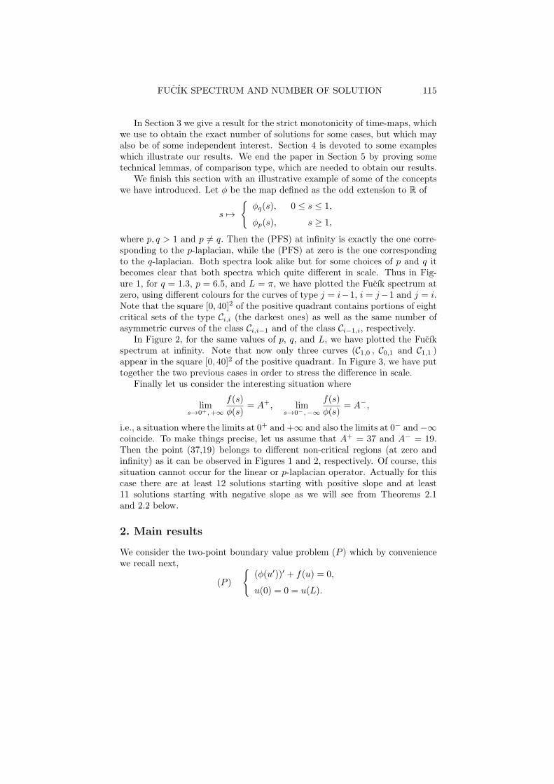
where p, q > 1 and p 6= q. Then the (PFS) at infinity is exactly the one corre-sponding to the p-laplacian, while the (PFS) at zero is the one correspondingto the q-laplacian. Both spectra look alike but for some choices of p and q itbecomes clear that both spectra which quite different in scale. Thus in Fig-ure 1, for q = 1.3, p = 6.5, and L = π, we have plotted the Fucık spectrum atzero, using different colours for the curves of type j = i−1, i = j−1 and j = i.Note that the square [0, 40]2 of the positive quadrant contains portions of eightcritical sets of the type Ci,i (the darkest ones) as well as the same number ofasymmetric curves of the class Ci,i−1 and of the class Ci−1,i, respectively.
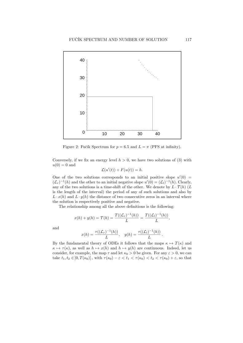
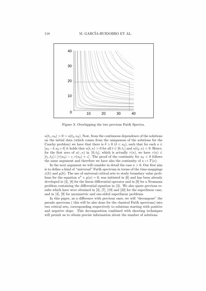
In Figure 2, for the same values of p, q, and L, we have plotted the Fucıkspectrum at infinity. Note that now only three curves (C1,0 , C0,1 and C1,1 )appear in the square [0, 40]2 of the positive quadrant. In Figure 3, we have puttogether the two previous cases in order to stress the difference in scale.
Finally let us consider the interesting situation where
lims→0+,+∞
f(s)
φ(s)= A+, lim
s→0−,−∞
f(s)
φ(s)= A−,
i.e., a situation where the limits at 0+ and +∞ and also the limits at 0− and−∞coincide. To make things precise, let us assume that A+ = 37 and A− = 19.Then the point (37,19) belongs to different non-critical regions (at zero andinfinity) as it can be observed in Figures 1 and 2, respectively. Of course, thissituation cannot occur for the linear or p-laplacian operator. Actually for thiscase there are at least 12 solutions starting with positive slope and at least11 solutions starting with negative slope as we will see from Theorems 2.1and 2.2 below.
2. Main results
We consider the two-point boundary value problem (P ) which by conveniencewe recall next,
(P )
{
(φ(u′))′ + f(u) = 0,
u(0) = 0 = u(L).
116 M. GARCIA-HUIDOBRO ET AL.
0
10
20
30
40
10 20 30 40
Figure 1: Fucık Spectrum for q = 1.3 and L = π (PFS at zero).
We begin our analysis by assuming (φ1) and (f1) only. Under these assumptionswe have that for each κ there is a unique solution u = u(·, κ) to the initialvalue problem
(φ(u′))′ + f(u) = 0, u(0) = 0, u′(0) = κ. (3)
This, indeed follows easily by writing equation (3) as an equivalent planarsystem and by using a result from [25]. Moreover, for any κ 6= 0, u(·, κ) is anontrivial periodic solution. We will denote by T (κ) its minimal period and byτ(κ) its first zero after t = 0.
Let us set Φ∗(s) =∫ s
0φ−1(ξ) dξ. Then L(s) = (Φ∗ ◦ φ)(s), where we re-
call L(s) = sφ(s) − Φ(s). As in [17], it is known that the following energyrelation holds
L(u′(t)) + F (u(t)) = L(κ), (4)
and it follows that u′(τ(κ)) = (Ll)−1(L(κ)) when κ > 0 and u′(τ(κ)) =
(Lr)−1(L(κ)) if κ < 0, so that
T (κ) = τ(κ) + τ((Ll)−1(L(κ))), for κ > 0
andT (κ) = τ(κ) + τ((Lr)
−1(L(κ))), for κ < 0.
FUCIK SPECTRUM AND NUMBER OF SOLUTION 117
0
10
20
30
40
10 20 30 40
Figure 2: Fucık Spectrum for p = 6.5 and L = π (PFS at infinity).
Conversely, if we fix an energy level h > 0, we have two solutions of (3) withu(0) = 0 and
L(u′(t)) + F (u(t)) = h.
One of the two solutions corresponds to an initial positive slope u′(0) =(Lr)
−1(h) and the other to an initial negative slope u′(0) = (Ll)−1(h). Clearly,
any of the two solutions is a time-shift of the other. We denote by L · T (h) (Lis the length of the interval) the period of any of such solutions and also byL · x(h) and L · y(h) the distance of two consecutive zeros in an interval wherethe solution is respectively positive and negative.
The relationship among all the above definitions is the following:
x(h) + y(h) = T (h) =T ((Lr)
−1(h))
L=T ((Ll)
−1(h))
L,
and
x(h) =τ((Lr)
−1(h))
L, y(h) =
τ((Ll)−1(h))
L.
By the fundamental theory of ODEs it follows that the maps κ 7→ T (κ) andκ 7→ τ(κ), as well as h 7→ x(h) and h 7→ y(h) are continuous. Indeed, let usconsider, for example, the map τ and let κ0 > 0 be given. For any ε > 0, we cantake t1, t2 ∈ ]0, T (κ0)[ , with τ(κ0) − ε < t1 < τ(κ0) < t2 < τ(κ0) + ε, so that
118 M. GARCIA-HUIDOBRO ET AL.
0
10
20
30
40
10 20 30 40
Figure 3: Overlapping the two previous Fucık Spectra.
u(t1, κ0) > 0 > u(t2, κ0). Now, from the continuous dependence of the solutionson the initial data (which comes from the uniqueness of the solutions for theCauchy problem) we have that there is δ > 0 (δ < κ0), such that for each κ ∈]κ0−δ, κ0+δ[ it holds that u(t, κ) > 0 for all t ∈ [0, t1] and u(t2, κ) < 0. Hence,for the first zero of u(·, κ) in ]0, t2], which is actually τ(κ), we have τ(κ) ∈]t1, t2[⊂ ]τ(κ0) − ε, τ(κ0) + ε[ . The proof of the continuity for κ0 < 0 followsthe same argument and therefore we have also the continuity of κ 7→ T (κ).
In the next argument we will consider in detail the case κ > 0. Our first aimis to define a kind of “universal” Fucık spectrum in terms of the time-mappingsx(h) and y(h). The use of universal critical sets to study boundary value prob-lems for the equation u′′ + g(u) = 0, was initiated in [6] and has been alreadydeveloped in [4], [8] for the linear differential operator and in [9] for a Neumannproblem containing the differential equation in (3). We also quote previous re-sults which have were obtained in [3], [7], [19] and [22] for the superlinear case,and in [4], [9] for asymmetric and one-sided superlinear problems.
In this paper, as a difference with previous ones, we will “decompose” thepseudo spectrum ( this will be also done for the classical Fucık spectrum) intotwo critical sets, corresponding respectively to solutions starting with positiveand negative slope. This decomposition combined with shooting techniqueswill permit us to obtain precise information about the number of solutions.
FUCIK SPECTRUM AND NUMBER OF SOLUTION 119
Lemma 2.1. Let φ and f satisfy (φ1) and (f1), respectively. Then, there existsκ > 0 such that problem (P ) has a solution with u′(0) = κ if and only if thereare n ∈ N and j ∈ {0, 1} such that
nx(h) + (n+ j − 1)y(h) = 1, h = L(κ). (5)
Moreover, in this case, u(·) has exactly 2n+ j − 2 zeros in ]0, L[ and there aren intervals in which u > 0 and n+ j − 1 intervals where u < 0.
The proof of this lemma is straightforward and is left to the reader. Basedon this result, we define the “critical lines”
H+i ={(x, y) ∈ (R+
0 )2 : ∃ (n ∈ N, j = 0, 1) : 2n+j−1 = i, nx+(n+j−1)y = 1}.
Thus, H+1 is the half-line x = 1, with y > 0; H+
2 is the open segment x+y = 1,with x, y > 0; H+
3 is the open segment 2x+ y = 1, with x, y > 0, and so forth.The superscript “+” is to remember that these critical lines are tied up withsolutions starting with positive slopes.
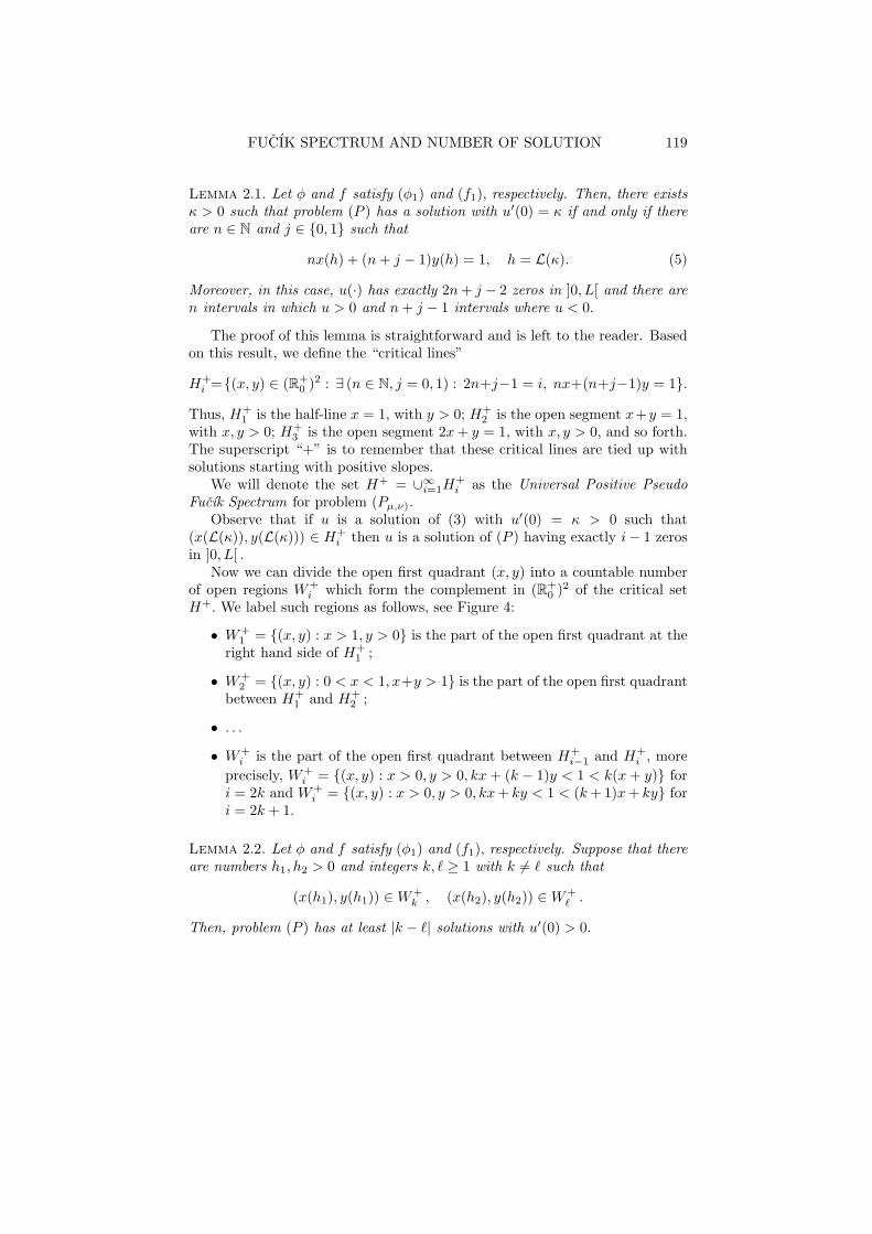
We will denote the set H+ = ∪∞i=1H
+i as the Universal Positive Pseudo
Fucık Spectrum for problem (Pµ,ν).Observe that if u is a solution of (3) with u′(0) = κ > 0 such that
(x(L(κ)), y(L(κ))) ∈ H+i then u is a solution of (P ) having exactly i− 1 zeros
in ]0, L[ .Now we can divide the open first quadrant (x, y) into a countable number
of open regions W+i which form the complement in (R+
0 )2 of the critical set
H+. We label such regions as follows, see Figure 4:
• W+1 = {(x, y) : x > 1, y > 0} is the part of the open first quadrant at the
right hand side of H+1 ;
• W+2 = {(x, y) : 0 < x < 1, x+y > 1} is the part of the open first quadrant
between H+1 and H+
2 ;
• . . .
• W+i is the part of the open first quadrant between H+
i−1 and H+i , more
precisely, W+i = {(x, y) : x > 0, y > 0, kx+ (k − 1)y < 1 < k(x+ y)} for
i = 2k and W+i = {(x, y) : x > 0, y > 0, kx+ ky < 1 < (k+1)x+ ky} for
i = 2k + 1.
Lemma 2.2. Let φ and f satisfy (φ1) and (f1), respectively. Suppose that thereare numbers h1, h2 > 0 and integers k, ℓ ≥ 1 with k 6= ℓ such that
(x(h1), y(h1)) ∈W+k , (x(h2), y(h2)) ∈W+
ℓ .
Then, problem (P ) has at least |k − ℓ| solutions with u′(0) > 0.
120 M. GARCIA-HUIDOBRO ET AL.
2H+
+
2W+
W+
W4+
H5
1H+
W
W1
+H3
4
+H4
+
+
3
0
0.5
1
0.5 1
Figure 4: Universal Positive Pseudo Fucık Spectrum.
Proof. Just to fix a case, let us assume that h1 < h2 and k < ℓ. By theassumptions, we have that the point (x(h1), y(h1)) is above H
+k and therefore
it is above any of the H+i for each i ≥ k. On the other hand, (x(h2), y(h2)) is
below H+ℓ−1 and hence it is also below any of the H+
i for each i ≤ ℓ− 1.Now, we fix an integer i ∈ [k, ℓ − 1] and observe that (x(h1), y(h1)) and
(x(h2), y(h2)) belong to different open components of (R+0 )
2 \ H+i . Since the
connected set {(x(h), y(h)): h1 ≤ h ≤ h2} has points in both components of(R+
0 )2 \ H+
i , it must intersect H+i at least once. By Lemma 2.1, this means
that there is solution of (P ) with positive slope at t = 0 and exactly i− 1 zerosin ]0, L[ . So, all together, there are at least ℓ− k solutions of (P ) starting witha positive slope.
Remark 2.1. Actually, the solutions given by the lemma are such that
α=min{(Lr)−1(h1), (Lr)
−1(h2)}<u′(0)<max{(Lr)
−1(h1), (Lr)−1(h2)}=β.
If τ(·) is strictly monotone in ]α, β[ and in ](Ll)−1((L(β)), (Ll)
−1((L(α))[ ,then the number of the solutions is exactly |k − ℓ|, for u′(0) = κ ranging in]α, β[ Indeed, if τ(·) is strictly increasing (decreasing), also the maps x(·) andy(·) are strictly increasing (decreasing) with respect to h.
Our argument continues by introducing some further maps and propertiesthat we need for the definition of the pseudo Fucık spectrum.

FUCIK SPECTRUM AND NUMBER OF SOLUTION 121
We deal, in first place, with the pseudo Fucık spectrum at infinity. Following[18], we assume conditions (φ1) and (φ∞) to hold and, moreover, that the limits
(T∞) :
T±1,∞(Λ) = lim
R→±∞
∣
∣
∣
∣
∣
∫ R
0
ds
L−1r (ΛΦ(R)− ΛΦ(s))
∣
∣
∣
∣
∣
and
T±2,∞(Λ) = lim
R→±∞
∣
∣
∣
∣
∣
∫ R
0
ds
L−1l (ΛΦ(R)− ΛΦ(s))
∣
∣
∣
∣
∣
exist. Furthermore, we define
T±∞(Λ) = T±
1,∞(Λ) + T±2,∞(Λ).
For each of the T±∞ , we assume that either T±
∞(Λ) = +∞ for all Λ, orit is continuous and strictly decreasing with respect to Λ ∈ R
+0 . Moreover
for this case, we assume that
limΛ→0+
T±∞(Λ) = +∞ and lim
Λ→+∞T±
∞(Λ) = 0.
Conditions under which these hypotheses are fulfilled are given in [17], [18]and [20] for φ odd and T finite.
Next we define the Positive Pseudo-Fucık Spectrum at infinity. For µ, ν > 0let us consider the problem (Pµ,ν) of the Introduction. Let us observe first thatin [18], for the case of φ an odd function, the four numbers T±
i,∞(Λ) are allthe same, finite and strictly positive, for any given Λ. Denoting this common
value by T∞(Λ) (it corresponds to T(Λ)2 as defined in (2)), we can describe the
(PFS) S (see the Introduction) as the union of the sets Ci,i−1 , Ci−1,i, and Ci,i ,for i ∈ N, contained in the positive (µ, ν)-quadrant, where
Ci,i−1 = {(µ, ν) | iT∞(µ) + (i− 1)T∞(ν) = L/2}
Ci−1,i = {(µ, ν) | (i− 1)T∞(µ) + iT∞(ν) = L/2}
Ci,i = {(µ, ν) | iT∞(µ) + iT∞(ν) = L/2}.
We want next to extend this definition to that of the Positive Pseudo-FucıkSpectrum (PPSF) at infinity, denoted by S+(∞), and where φ is not necessarilyodd. We set
S+(∞) = ∪∞i=1C
+i (∞),
where we consider only the case of solutions with positive (and large) slopes att = 0. Here,
C+1 (∞) = {(µ, ν) ∈ (R+
0 )2 : T+
∞(µ) = L},
C+2 (∞) = {(µ, ν) ∈ (R+
0 )2 : T+
∞(µ) + T−∞(ν) = L},
122 M. GARCIA-HUIDOBRO ET AL.
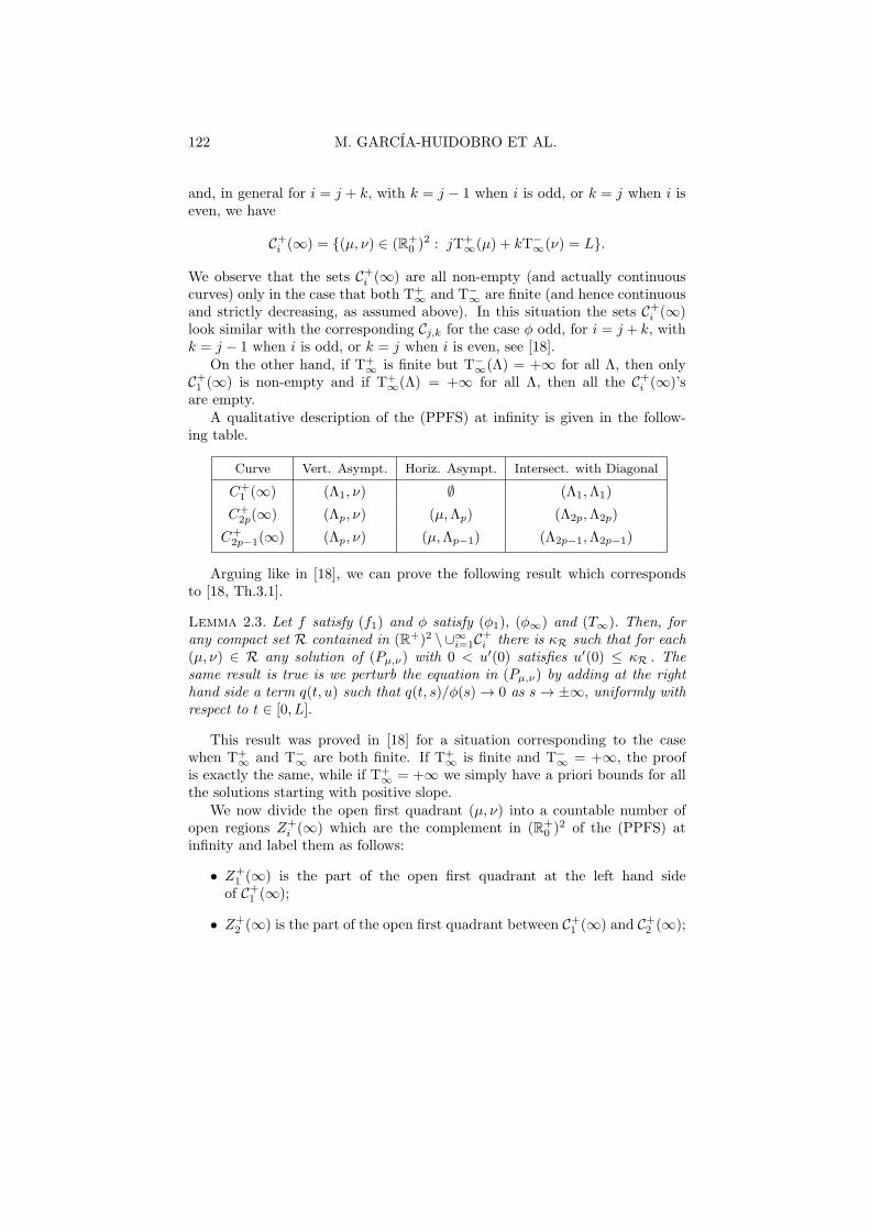
and, in general for i = j + k, with k = j − 1 when i is odd, or k = j when i iseven, we have
C+i (∞) = {(µ, ν) ∈ (R+
0 )2 : jT+
∞(µ) + kT−∞(ν) = L}.
We observe that the sets C+i (∞) are all non-empty (and actually continuous
curves) only in the case that both T+∞ and T−
∞ are finite (and hence continuousand strictly decreasing, as assumed above). In this situation the sets C+
i (∞)look similar with the corresponding Cj,k for the case φ odd, for i = j + k, withk = j − 1 when i is odd, or k = j when i is even, see [18].
On the other hand, if T+∞ is finite but T−
∞(Λ) = +∞ for all Λ, then onlyC+1 (∞) is non-empty and if T+
∞(Λ) = +∞ for all Λ, then all the C+i (∞)’s
are empty.A qualitative description of the (PPFS) at infinity is given in the follow-
ing table.
Curve Vert. Asympt. Horiz. Asympt. Intersect. with Diagonal
C+1 (∞) (Λ1, ν) ∅ (Λ1,Λ1)
C+2p(∞) (Λp, ν) (µ,Λp) (Λ2p,Λ2p)
C+2p−1(∞) (Λp, ν) (µ,Λp−1) (Λ2p−1,Λ2p−1)
Arguing like in [18], we can prove the following result which correspondsto [18, Th.3.1].
Lemma 2.3. Let f satisfy (f1) and φ satisfy (φ1), (φ∞) and (T∞). Then, forany compact set R contained in (R+)2 \ ∪∞
i=1C+i there is κR such that for each
(µ, ν) ∈ R any solution of (Pµ,ν) with 0 < u′(0) satisfies u′(0) ≤ κR . Thesame result is true is we perturb the equation in (Pµ,ν) by adding at the righthand side a term q(t, u) such that q(t, s)/φ(s) → 0 as s→ ±∞, uniformly withrespect to t ∈ [0, L].
This result was proved in [18] for a situation corresponding to the casewhen T+
∞ and T−∞ are both finite. If T+
∞ is finite and T−∞ = +∞, the proof
is exactly the same, while if T+∞ = +∞ we simply have a priori bounds for all
the solutions starting with positive slope.We now divide the open first quadrant (µ, ν) into a countable number of
open regions Z+i (∞) which are the complement in (R+
0 )2 of the (PPFS) at
infinity and label them as follows:
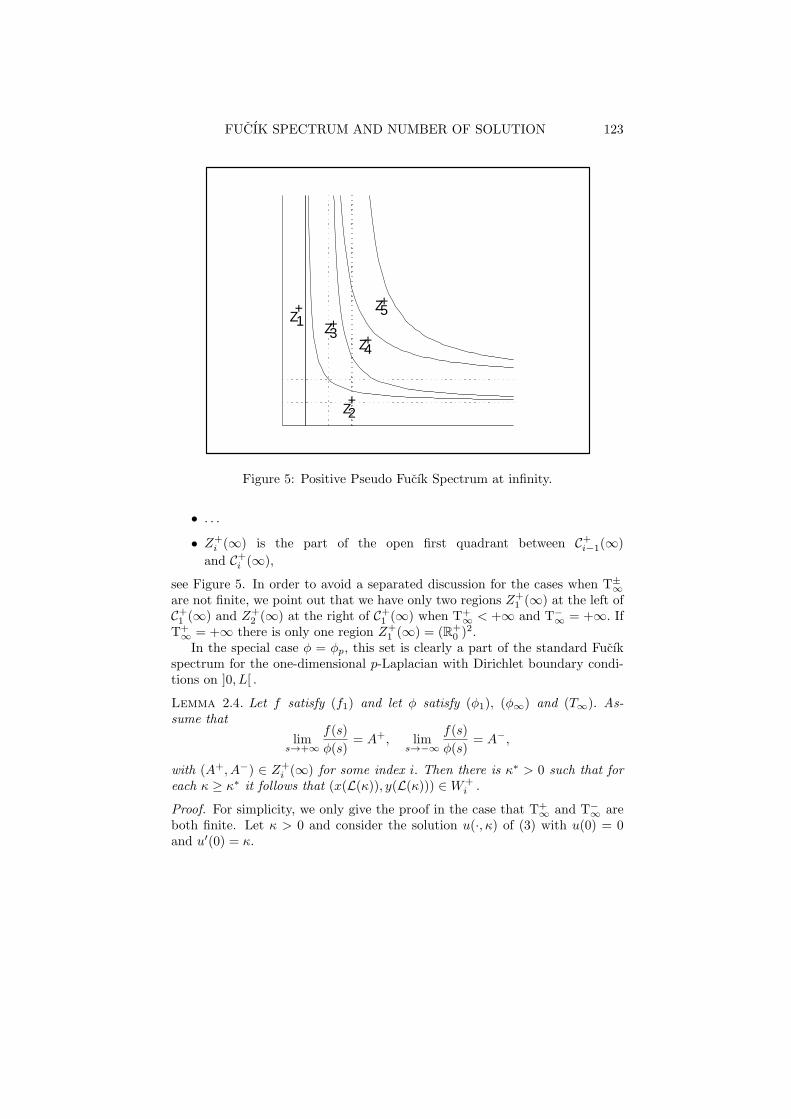
• Z+1 (∞) is the part of the open first quadrant at the left hand side
of C+1 (∞);
• Z+2 (∞) is the part of the open first quadrant between C+
1 (∞) and C+2 (∞);
FUCIK SPECTRUM AND NUMBER OF SOLUTION 123
+
Z
2
+4Z
Z
Z ++1
+
3Z5
Figure 5: Positive Pseudo Fucık Spectrum at infinity.
• . . .
• Z+i (∞) is the part of the open first quadrant between C+
i−1(∞)
and C+i (∞),
see Figure 5. In order to avoid a separated discussion for the cases when T±∞
are not finite, we point out that we have only two regions Z+1 (∞) at the left of
C+1 (∞) and Z+
2 (∞) at the right of C+1 (∞) when T+
∞ < +∞ and T−∞ = +∞. If
T+∞ = +∞ there is only one region Z+
1 (∞) = (R+0 )
2.In the special case φ = φp, this set is clearly a part of the standard Fucık
spectrum for the one-dimensional p-Laplacian with Dirichlet boundary condi-tions on ]0, L[ .
Lemma 2.4. Let f satisfy (f1) and let φ satisfy (φ1), (φ∞) and (T∞). As-sume that
lims→+∞
f(s)
φ(s)= A+, lim
s→−∞
f(s)
φ(s)= A−,
with (A+, A−) ∈ Z+i (∞) for some index i. Then there is κ∗ > 0 such that for
each κ ≥ κ∗ it follows that (x(L(κ)), y(L(κ))) ∈W+i .
Proof. For simplicity, we only give the proof in the case that T+∞ and T−
∞ areboth finite. Let κ > 0 and consider the solution u(·, κ) of (3) with u(0) = 0and u′(0) = κ.
124 M. GARCIA-HUIDOBRO ET AL.
First of all, we claim that the distance of two consecutive zeros of u inan interval where u > 0 is given by T+
∞(A+) + ε1(κ) and the distance of twoconsecutive zeros of u for an interval where u < 0 is given by T−
∞(A−)+ ε2(κ),where ε1(κ) → 0 and ε2(κ) → 0 as κ → +∞. Hence, we have that x(L(κ)) −L−1 · T+
∞(A+) → 0 and y(L(κ))− L−1 · T−∞(A−) → 0 as κ→ +∞.
To see this, we observe that for each ε > 0 there is Mε > 0 such that
(A+ − ε)φ(s) ≤ f(s) ≤ (A+ + ε)φ(s), ∀ s ≥Mε
and(A+ − ε)|φ(s)| ≤ |f(s)| ≤ (A+ + ε)|φ(s)|, ∀ s ≤ −Mε .
Hence, by Corollary A.1 in the appendix, and since by the energy relation (4),maxu, |minu| → +∞ as κ→ +∞, we find that
T+∞(A+ − ε) ≤ lim inf
κ→+∞τ(κ) ≤ lim sup
κ→+∞τ(κ) ≤ T+
∞(A+ + ε).
(Here the assumption (T∞) which guarantees the existence of the limitsT+
∞(A+ ± ε) has been used.) Then, from these inequalities and the continuityof the function T+
∞ , we immediately obtain that
limκ→+∞
τ(κ) = limh→+∞
L · x(h) = T+∞(A+).
In a completely similar manner, one can see that
limκ→+∞
τ(L−1(κ)) = limh→+∞
L · y(h) = T−∞(A−),
concluding the proof of our claim.Suppose next that
(A+, A−) ∈ Z+i (∞) for some i ∈ N.
Without loss of generality we assume also that i > 1 and that i = 2k is aneven number (the case i = 1 is simpler as it requires only a one-sided estimate).This means that (A+, A−) is above the curve
C+i−1(∞) = {(µ, ν) ∈ (R+
0 )2 : kT+
∞(µ) + (k − 1)T−∞(ν) = L}
and below the curve
C+i (∞) = {(µ, ν) ∈ (R+
0 )2 : kT+
∞(µ) + kT−∞(ν) = L}
and hence,
L < kT+∞(A+) + kT−
∞(A−), kT+∞(A+) + (k − 1)T−
∞(A−) < L.
FUCIK SPECTRUM AND NUMBER OF SOLUTION 125
Now, using the estimates in [18] for the time-mappings recalled at the beginningof this proof, we find that
kx(L(κ)) + ky(L(κ)) → kT+
∞(A+)
L+ k
T−∞(A−)
L> 1
and
kx(L(κ)) + (k − 1)y(L(κ)) → kT+
∞(A+)
L+ (k − 1)
T−∞(A−)
L< 1
as κ → +∞. This, in turns, implies that there is κ∗ > 0 such that for eachκ > κ∗ the pair (x(L(κ)), y(L(κ))) belongs to a compact subset of W+
i .
The case i is an odd number is clearly treated in the same way and thereforeit is omitted.
By repeating the same reasoning at zero, and using the estimates in [20], wecan define the Positive Pseudo-Fucık Spectrum at zero S+(0) as the union of acountable number of critical curves C+
i (0) obtained in a similar manner as forthe critical sets of the (PPFS) at infinity, but this time, with the asymptoticestimates made at zero.
More precisely let us assume the conditions (φ1) and (φ0), andthat the limits
(T0) :
T±1,0(Λ) = lim
R→0±
∣
∣
∣
∣
∣
∫ R
0
ds
L−1r (ΛΦ(R)− ΛΦ(s))
∣
∣
∣
∣
∣
and
T±2,0(Λ) = lim
R→0±
∣
∣
∣
∣
∣
∫ R
0
ds
L−1l (ΛΦ(R)− ΛΦ(s))
∣
∣
∣
∣
∣
exist. Furthermore, define
T±0 (Λ) = T±
1,0(Λ) + T±2,0(Λ),
and assume that for each of the T±0 , either T±
0 (Λ) = +∞ for all Λ, or itis continuous and strictly decreasing with respect to Λ ∈ R
+0 . Moreover
we assume that,
limΛ→0+
T±0 (Λ) = +∞ and lim
Λ→+∞T±
0 (Λ) = 0.
Similarly to Lemma 2.3, we can prove the following lemma.

126 M. GARCIA-HUIDOBRO ET AL.
Lemma 2.5. Let f satisfy (f1) and let φ satisfy (φ1), (φ0) and (T0). Then, forany compact set K contained in (R+
0 )2 \ ∪∞
i=1C+i (0) there is κR such that for
each (µ, ν) ∈ R any solution of (Pµ,ν) with 0 < u′(0) satisfies u′(0) ≥ κR .The same result is true is we perturb the equation in (Pµ,ν) by adding a termq(t, u) at the right hand side such that q(t, s)/φ(s) → 0 as s → 0, uniformlywith respect to t ∈ [0, L].
As before, we can define the corresponding regions in the complementaryparts of the (PPFS) at zero. Accordingly, we denote by Z+
i (0) the componentsin the complement of the (PPFS) at zero.
We have the following result which is analogous to Lemma 2.4 and whoseproof follows the same lines of that of Lemma 2.4, by using the comparisonresult of Lemma A.1.
Lemma 2.6. Let f satisfy (f1) and let φ satisfy (φ1), (φ0) and (T0). Assume that
lims→0+
f(s)
φ(s)= a+, lim
s→0−
f(s)
φ(s)= a−,
with (a+, a−) ∈ Z+i (0) for some index i. Then there is κ∗ > 0 such that for
each 0 < κ ≤ κ∗, it follows that (x(L(κ)), y(L(κ))) ∈W+i .
We are now in a position to state our first main result.
Theorem 2.1. Let f satisfy (f1) and let φ satisfy (φ1), (φ0), (φ∞) and (T0),(T∞). Suppose that there are positive numbers a+, a−, A+, A− such that
lims→0+
f(s)
φ(s)= a+, lim
s→0−
f(s)
φ(s)= a−
and
lims→+∞
f(s)
φ(s)= A+, lim
s→−∞
f(s)
φ(s)= A−.
Assume also that there are k, ℓ ∈ N with k 6= ℓ with (a+, a−) ∈ Z+k (0) and
(A+, A−) ∈ Z+ℓ (∞). Then, problem (P ) has at least |k − ℓ| solutions with
u′(0) > 0.
Proof. The proof is a direct consequence of the Lemmas 2.4, 2.6, and 2.2, and byusing the Positive Pseudo Fucık Spectrum (PPFS) at zero and at infinity.
At this point we can establish corresponding results for solutions of (3) withκ < 0, by using a similar reasoning. To this end, with x(h) and y(h) as definedabove, we need the following lemma which will take the place of Lemma 2.1.
FUCIK SPECTRUM AND NUMBER OF SOLUTION 127
Lemma 2.7. Let φ and f satisfy (φ1) and (f1), respectively. Then, there existsκ < 0 such that problem (P ) has a solution with u′(0) = κ if and only if thereare n ∈ N and j ∈ {0, 1} such that
(n+ j − 1)x(h) + ny(h) = 1, h = L(κ). (6)
Moreover, in this case, u(·) has exactly 2n+ j − 2 zeros in ]0, 1[ and also thereare n intervals in which u < 0 and n+ j − 1 intervals where u > 0.
From this result we can define, as before, the critical lines:
H−i ={(x, y) ∈ (R+
0 )2 : ∃ (n ∈ N, j = 0, 1) : 2n+j−1 = i, (n+j−1)x+ny = 1}.
Thus H−1 is the half-line y = 1, with x > 0; H−
2 is the open segment x+ y = 1,with x, y > 0; H−
3 is the open segment x+ 2y = 1, with x, y > 0, and so forth.The superscript “-” is to remember that these critical lines are related withsolutions starting with negative slopes.
We will denote the set H− = ∪∞i=1H
−i as the Universal Negative Pseudo
Fucık Spectrum.As before, we can divide the open first quadrant (x, y) into a countable
number of open regions W−i which are the complement in (R+
0 )2 of the critical
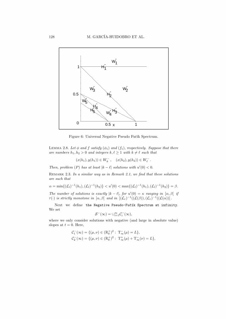
set H−. We label such zones as follows, see Figure 6:
• W−1 = {(x, y) : x > 0, y > 1} is the part of the open first quadrant
above H−1 ;
• W−2 = {(x, y) : x+y > 1, 0 < y < 1} is the part of the open first quadrant
between H−1 and H−
2 ;
• . . .
• W−i is the part of the open first quadrant between H−
i−1 and H−i and,
more precisely, we have W−i = {(x, y) : x > 0, y > 0, (k − 1)x+ ky < 1 <
k(x + y)} for i = 2k and W−i = {(x, y) : x > 0, y > 0, kx + ky < 1 <
kx+ (k + 1)y} for i = 2k + 1.
Remark 2.2. The set H = H+ ∪H− has the same shape like the set F drawnin [4, p.874]. It represents a “universal” model of Fucık spectrum for the two-point boundary value problem in terms of time-maps. What we have done hereis to distinguish the parts H+ and H− in H in order to treat separately thesolutions with positive slope and those with negative slope. The same procedureis feasible for the standard Fucık spectrum C which splits as a “positive” part(concerning solutions with positive slope at t = 0) and a “negative” part (forthe solutions with negative slope at t = 0).
The following lemma is the equivalent to Lemma 2.2, it is proved similarly.
128 M. GARCIA-HUIDOBRO ET AL.
-1W
-H
-
W
5-
5-
H
-H1
2
4H
-
H3-
W
3-
W4
2-
W
0
0.5
1
0.5 1x
Figure 6: Universal Negative Pseudo Fucık Spectrum.
Lemma 2.8. Let φ and f satisfy (φ1) and (f1), respectively. Suppose that thereare numbers h1, h2 > 0 and integers k, ℓ ≥ 1 with k 6= ℓ such that
(x(h1), y(h1)) ∈W−k , (x(h2), y(h2)) ∈W−
ℓ .
Then, problem (P ) has at least |k − ℓ| solutions with u′(0) < 0.
Remark 2.3. In a similar way as in Remark 2.1, we find that these solutionsare such that
α = min{(Ll)−1(h1), (Ll)
−1(h2)} < u′(0) < max{(Ll)−1(h1), (Ll)
−1(h2)} = β.
The number of solutions is exactly |k − ℓ|, for u′(0) = κ ranging in ]α, β[ ifτ(·) is strictly monotone in ]α, β[ and in ](Lr)
−1((L(β)), (Lr)−1((L(α))[ .
Next we define the Negative Pseudo-Fucık Spectrum at infinity.We set
S−(∞) = ∪∞i=1C
−i (∞),
where we only consider solutions with negative (and large in absolute value)slopes at t = 0. Here,
C−1 (∞) = {(µ, ν) ∈ (R+
0 )2 : T−
∞(µ) = L},
C−2 (∞) = {(µ, ν) ∈ (R+
0 )2 : T+
∞(µ) + T−∞(ν) = L},
FUCIK SPECTRUM AND NUMBER OF SOLUTION 129
and, in general, for i = k+ l with k = l− 1 (when i is odd) or k = l (when i iseven), we have
C−i (∞) = {(µ, ν) ∈ (R+
0 )2 : kT+
∞(µ) + lT−∞(ν) = L}.
By this definition, C−i (∞) = C+
i (∞), when i is even.As before the sets C−
i (∞) are all non-empty (and actually continuous curves)only in the case that both T+
∞ and T−∞ are finite (and hence continuous and
decreasing by assumption). On the other hand, if T−∞ is finite but T+
∞(Λ) =+∞ for all Λ, then only C−
1 (∞) is non-empty and if T−∞(Λ) = +∞ for all Λ,
then all the C−i (∞)’s are empty.
A qualitative description of the (NPFS) at infinity is given in the follow-ing table.
Curve Vert. Asympt. Horiz. Asympt. Intersect. with Diagonal
C−1 (∞) (µ,Λ1) ∅ (Λ1,Λ1)
C−2p(∞) (Λp, ν) (µ,Λp) (Λ2p,Λ2p)
C−2p−1(∞) (Λp−1, ν) (µ,Λp) (Λ2p−1,Λ2p−1)
Corresponding to Lemma 2.3, we now have.
Lemma 2.9. Let f satisfy (f1) and let φ satisfy (φ1), (φ∞) and (T∞). Then,for any compact set R contained in (R+)2 \ ∪∞
i=1C−i there is κR such that for
each (µ, ν) ∈ R any solution of (Pµ,ν) with u′(0) < 0 satisfies |u′(0)| ≤ κR .The same result is true is we perturb the equation in (Pµ,ν) by adding at theright hand side a term q(t, u) such that q(t, s)/φ(s) → 0 as s→ ±∞, uniformlywith respect to t ∈ [0, L].
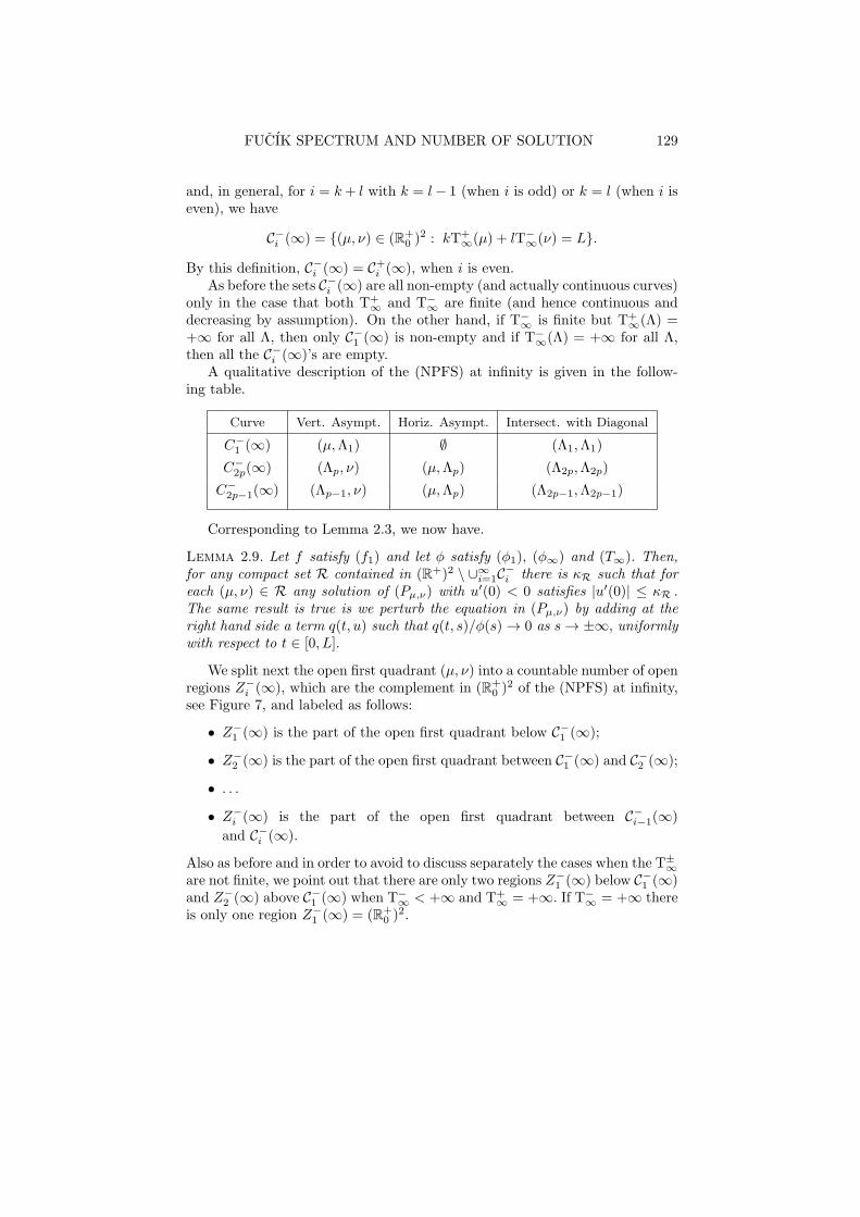
We split next the open first quadrant (µ, ν) into a countable number of openregions Z−
i (∞), which are the complement in (R+0 )
2 of the (NPFS) at infinity,see Figure 7, and labeled as follows:
• Z−1 (∞) is the part of the open first quadrant below C−
1 (∞);
• Z−2 (∞) is the part of the open first quadrant between C−
1 (∞) and C−2 (∞);
• . . .
• Z−i (∞) is the part of the open first quadrant between C−
i−1(∞)
and C−i (∞).
Also as before and in order to avoid to discuss separately the cases when the T±∞
are not finite, we point out that there are only two regions Z−1 (∞) below C−
1 (∞)and Z−
2 (∞) above C−1 (∞) when T−
∞ < +∞ and T+∞ = +∞. If T−
∞ = +∞ thereis only one region Z−
1 (∞) = (R+0 )
2.
130 M. GARCIA-HUIDOBRO ET AL.
-
-
-
-
-
Z
Z3
1
5Z
Z
4
2Z
Figure 7: Negative Pseudo Fucık Spectrum at infinity.
The following lemma is the counterpart of Lemma 2.4 and it is proved inthe same form.
Lemma 2.10. Let f satisfy (f1) and let φ satisfy (φ1), (φ∞) and (T∞). As-sume that
lims→+∞
f(s)
φ(s)= B+, lim
s→−∞
f(s)
φ(s)= B−,
with (B+, B−) ∈ Z−i (∞) for some index i. Then there is κ∗ > 0 such that for
each κ ≤ −κ∗ it follows that (x(L(κ)), y(L(κ))) ∈W−i .
Remark 2.4. The critical set S defined in [18], that is the (PFS) at infinity,is exactly S+(∞) ∪ S−(∞).
By repeating the argument, and using estimates like in [5] we can define theNegative Pseudo-Fucık Spectrum at zero C−(0) as the union of a count-able number of critical curves C−
i (0) defined in a similar manner as the criticalsets of the (NPFS) at infinity, but, this time, with the estimates made at zero.Also we can define the corresponding zones Z−
i (0) as the complementary partsof the (NPFS) at zero.
Similarly to Lemmas 2.9 and 2.10, we now have.
Lemma 2.11. Let f satisfy (f1) and let φ satisfy (φ1), (φ0) and (T0). Then, forany compact set K contained in (R+)2 \ ∪∞
i=1C−i (0) there is κR such that for

FUCIK SPECTRUM AND NUMBER OF SOLUTION 131
each (µ, ν) ∈ R any solution of (Pµ,ν) with u′(0) < 0 satisfies |u′(0)| ≥ κR .The same result is true is we perturb the equation in (Pµ,ν) by adding at theright hand side a term q(t, u) such that q(t, s)/φ(s) → 0 as s → 0, uniformlywith respect to t ∈ [0, L].
Lemma 2.12. Let f satisfy (f1) and let φ satisfy (φ1), (φ0) and (T0). As-sume that
lims→0+
f(s)
φ(s)= b+, lim
s→0−
f(s)
φ(s)= b−,
with (b+, b−) ∈ Z−i (0) for some index i. Then there is κ∗ > 0 such that for
each −κ∗ ≤ κ < 0 it follows that (x(L(κ)), y(L(κ))) ∈W−i .
We thus have reached a point where we can establish and prove our secondmain theorem.
Theorem 2.2. Let f satisfy (f1) and let φ satisfy (φ1), (φ0), (φ∞) and (T0),(T∞). Suppose that there are positive numbers b+, b−, B+, B− such that
lims→0+
f(s)
φ(s)= b+, lim
s→0−
f(s)
φ(s)= b−
and
lims→+∞
f(s)
φ(s)= B+, lim
s→−∞
f(s)
φ(s)= B−.
Assume also that there are k, ℓ ∈ N with k 6= ℓ with (b+, b−) ∈ Z−k (0)
and (B+, B−) ∈ Z−ℓ (∞). Then, problem (P ) has at least |k − ℓ| solutions
with u′(0) < 0.
Proof. Direct consequence of Lemmas 2.11, 2.12, and 2.8.
Note that given a pair (µ, ν) ∈ (R+0 )
2, not belonging to the critical set atzero S+(0), we can determine the region Z+
i (0) to which it belongs, by thefollowing criterion. Let us set
ρ(0) =L
T+0 (µ) + T−
0 (ν)
and observe that there is only one integer, say j, belonging to the open interval
]
ρ(0)−T+0 (µ)
T+0 (µ) + T−
0 (ν), ρ(0) +
T−0 (ν)
T+0 (µ) + T−
0 (ν)
[
.
Then, we have that (µ, ν) belongs to Z+2j(0) or Z
+2j+1(0), according to whether
j > ρ(0) or j < ρ(0).
132 M. GARCIA-HUIDOBRO ET AL.
Avoiding to consider the semi-trivial cases in which one or both of the twomaps T±
0 are infinite, we observe that ρ(0) as a function of µ or ν is continuous,strictly increasing and such that ρ(0) → 0 as µ → 0+ or ν → 0+. Moreoverρ(0) → L
T−
0(ν)
as µ → +∞ and ρ(0) → L
T+
0(µ)
as µ → +∞. On the other hand,
for α(0) =T
+
0(µ)
T+
0(µ)+T
−
0(ν)
, we have that 0 < α(0) < 1, with α(0) decreasing in
µ and increasing in ν and such that α(0) → 1 as µ → 0+, or µ → +∞ andα(0) → 0 as µ→ +∞, or ν → 0+.
Clearly, the same procedure can be followed in order to determine the regionZ+i (∞) to which the pair (µ, ν) belongs.
Similarly, given a pair (µ, ν) ∈ (R+0 )
2 not belonging to the critical set atzero S−(0), we can determine the region Z−
i (0) it belongs, by the followingcriterion. Let us set
ρ(0) =L
T+0 (µ) + T−
0 (ν),
and as before observe that there is only one integer, say j, belonging to theopen interval
]
ρ(0)−T−0 (ν)
T+0 (µ) + T−
0 (ν), ρ(0) +
T+0 (µ)
T+0 (µ) + T−
0 (ν)
[
.
Then, we have that (µ, ν) belongs to Z−2j(0) or Z
−2j+1(0), according to whether
j > ρ+(0) or j < ρ+(0).
The same procedure can be followed in order to determine the region Z−i (∞)
the pair (µ, ν) belongs to.
Remark 2.5. In the proof of the main theorems, it is not important that the lim-iting pairs (a+, a−) and (A+, A−) in Theorem 2.1, or (b+, b−), and (B+, B−)in Theorem 2.2 be in “nonresonance” zones out of the (PFS) sets. What re-ally matters is that there is a suitable gap between the corresponding positionsof these limits at zero and at infinity with respect to the universal Fucık spec-trum. This situation reminds the occurrence of a twist condition between zeroand infinity which permits the application of the Poincare-Birkhoff fixed pointtheorem in the periodic case [11].
In view of the above remark, the following rule can be given.
The set U+ := {H+i ,W+
i : i ∈ N} represents a partition of (R+0 )
2 . Giventwo points P,Q ∈ (R+
0 )2 , we have that the number of transverse intersections
between the open segment ]P,Q[ and the critical lines ∪∞i=1H
+i depends only
on which of the classes of the above partition P and Q belong to (notice that, inthis way, if P and Q are both on the same critical line H+
i , then the intersectioncounts like zero).

FUCIK SPECTRUM AND NUMBER OF SOLUTION 133
The sets M+(0) := {C+i (0) , Z+
i (0) : i ∈ N} and M+(∞) :={C+
i (∞) , Z+i (∞) : i ∈ N} also determine a partition of (R+
0 )2 . We can de-
fine now the mapsM+(0) → U+, M+(∞) → U+
byC+i (0), C+
i (∞) 7→ H+i and Z+
i (0), Z+i (∞) 7→W+
i .
Note that these maps make a correspondence between curves to lines and opensets to open sets.
Take a point (a, b) ∈ (∪∞i=1C
+i (0)) ∪ (∪∞
i=1Z+i (0)).We can associate to (a, b)
the set in M+(0) to which it belongs and hence, to this one, the set in U+
which is associated to it via the above map. Call this set [(a, b)]. Similarly,given a point (A,B) ∈ (∪∞
i=1C+i (∞)) ∪ (∪∞
i=1Z+i (∞)) we can map it to a set
[(A,B)] ∈ U+, where [(A,B)] is the set corresponding to that one in M+(∞)to which (A,B) belongs. Since, as observed before, the number of transverseintersections of the open segment ]P,Q[ with the set ∪∞
i=1H+i is the same for
each P ∈ [(a, b)] and Q ∈ [(A,B)], we have that this number is well determinedby the initial choice of the pairs (a, b) and (A,B). We denote this number byi+[(a, b), (A,B)] and call it the positive intersection index for the pairs (a, b)and (A,B).
We remark that this definition requires that the pairs (a, b) and (A,B) are“thought” in relation with the (PPFS) at zero and at infinity, respectively.
In a similar manner, one can define the partitions U−, M−(0), M−(∞) of(R+
0 )2 and the maps
C−i (0), C−
i (∞) 7→ H−i and Z−
i (0), Z−i (∞) 7→W−
i ,
in order to define an index i−[(c, d), (C,D)] as the negative intersection indexfor the pairs (c, d) and (C,D), where (c, d) is related to the (NPFS) at zeroand (CD) to the (NPFS) at infinity.
We point out that this procedure works also in the “degenerate” case inwhich some of the T±
0 (Λ) or T±∞(Λ) considered in (T0) and in (T∞) is constantly
equal to infinity. In this situation, some of the maps M±(0),M±(0) → U± willbe not surjective, but the definition of the intersection indexes is well posed too.
Then, we have:
Theorem 2.3. Let f satisfy (f1) and let φ satisfy (φ1), (φ0), (φ∞) and (T0),(T∞). Suppose that there are positive numbers d+, d−, D+, D− such that
lims→0+
f(s)
φ(s)= d+, lim
s→0−
f(s)
φ(s)= d−
and
lims→+∞
f(s)
φ(s)= D+, lim
s→−∞
f(s)
φ(s)= D−.

134 M. GARCIA-HUIDOBRO ET AL.
Then, problem (P ) has at least so many solutions with u′(0) > 0 like the positiveintersection index i+[(d+, d−), (D+, D−)] and at least so many solutions withu′(0) < 0 like the negative intersection index i−[(d+, d−), (D+, D−)].
3. A result for strictly monotone time-mappings
We present in this section some suitable conditions under which we have astrictly monotone time-map. Hence, according to the remarks after Lemmas2.2 and 2.8, they can be applied to obtain an exact number of solutions, .
We shall confine ourselves only to the consideration of τ(κ) for κ > 0. Thesituation in which κ < 0 is completely symmetric and therefore can be discussedusing the same arguments.
For simplicity, we suppose that φ : R → R is an odd increasing homeomor-phism which is of class C1 in R
+0 and such that
(φ2) lims→0+
s2φ′(s) = 0
and we also assume that f : R → R satisfy (f1). Let u(·) be a solution of (3)for some κ > 0.
From the energy relation (4) we can compute the distance τ(κ) of twoconsecutive zeros of u in an interval where u > 0 by the formula
τ(κ) = 2
∫ R
0
ds
L−1r (F (R)− F (s))
, with F (R) = L(κ), R > 0,
where the number “2” comes from the fact that, by the symmetry of φ, wehave that the time from t = 0 to the point of maximum of u is the same likethe time from the point of maximum of u and t = τ(κ).
For convenience in the next proof, we also introduce the function
Ψ(s) := φ′(L−1r (s))(L−1
r (s))2,
which, by the assumptions on φ, is defined and continuous for every s > 0 and,by (φ2) can be extended by continuity to the origin, putting Ψ(0) = 0.
Then, the following result can be proved:
Lemma 3.1. Assume (φ2) and suppose that the function Ψ is convex (respec-tively, concave) in R
+. Then, the map κ 7→ τ(κ) is strictly decreasing (respec-tively, strictly increasing) if the map s 7→ sf(s)−Ψ(F (s)) is strictly increasing(respectively, strictly decreasing).
Proof. First of all, via the change of variables s = Rt, we write the integralfor τ(κ) as
τ(κ) = 2
∫ 1
0
Rdt
L−1r (F (R)− F (Rt))
,
FUCIK SPECTRUM AND NUMBER OF SOLUTION 135
so that, in order to prove that τ(·) is strictly decreasing (respectively, strictlyincreasing) for κ in a certain interval, say κ ∈ ]α, β[ , with 0 ≤ α < β ≤ +∞,we may prove that, for each t ∈ ]0, 1[ the map R 7→ (L−1
r (F (R) − F (Rt)))/Ris strictly increasing (or strictly decreasing) on ]α1, β1[ , where we have setα1 = F−1
r (L(α)) and β1 = F−1r (L(β)). To do this, we compute the derivative
with respect to R for any fixed t ∈ ]0, 1[ . Then, at the numerator we find
Rf(R)−Rtf(Rt)
L′(L−1r (F (R)− F (Rt)))
− L−1r (F (R)− F (Rt)).
Recalling that L′(ξ) = ξφ′(ξ) and the definition of Ψ, we conclude that τ isstrictly decreasing (strictly increasing) in ]α, β[ , if
Rf(R)−Rtf(Rt)−Ψ(F (R)− F (Rt)) > 0 (7)
holds every R ∈ ]α1, β1[ and all t ∈ ]0, 1[ . Now, according to the assumption,we have that Ψ is a convex function and recall also that Ψ(0) = 0. Fromthis, it follows that Ψ(a + b) ≥ Ψ(a) + Ψ(b) for all a, b ≥ 0 and therefore,Ψ(x − y) ≤ Ψ(x) − Ψ(y) for all 0 < y < x. Hence, we have that Ψ(F (R) −F (Rt)) ≤ Ψ(F (R)) − Ψ(F (Rt)) holds for every R ∈ ]α1, β1[ and all t ∈ ]0, 1[and therefore, in order to prove (7) it will be sufficient to prove that
Rf(R)−Rtf(Rt)− [Ψ(F (R))−Ψ(F (Rt))] > 0
holds for every R ∈ ]α1, β1[ and all t ∈ ]0, 1[ .Now, to have this last inequality satisfied it will be enough to have that the
function R 7→ Rf(R)−Ψ(F (R)) is strictly increasing on the interval ]0, β1[ .In case that the function Ψ is concave, we use the inequality Ψ(x − y) ≥
Ψ(x) − Ψ(y) for all 0 < y < x and obtain that the time-mapping is strictlyincreasing on ]α, β[ provided that the map R 7→ Rf(R)−Ψ(F (R)) is strictlydecreasing in the interval ]0, β1[ .
Note that if φ is of class C2 in R+0 , then the map Ψ is convex (respectively,
concave) provided that sφ′′(s)/φ′(s) is increasing (respectively, decreasing) onR
+0 . In the special case of φ = φp , for some p > 1, we have that sφ′′(s)/φ′(s)
is a positive constant.An elementary application of Lemma 3.1 is the following:
Corollary 3.1. For φ = φp , with p > 1, the following holds: The map κ 7→
τ(κ) is strictly decreasing (respectively, strictly increasing) if the map s 7→ f(s)sp−1
is strictly increasing (respectively, strictly decreasing).
Proof. In this case, by a direct computation, we have that Ψ(s) = ps, sothat all the assumptions on Ψ are satisfied and the auxiliary function s 7→sf(s) − Ψ(F (s)) takes the form of sf(s) − pF (s), which, in turn, is strictly
increasing (respectively, strictly decreasing) if the map s 7→ f(s)sp−1 is strictly
increasing (respectively, strictly decreasing), too.
136 M. GARCIA-HUIDOBRO ET AL.
Corollary 3.1 extends a classical result obtained by Opial [24] for the casep = 2. Other estimates for the time-mappings associated to the φp or theφ-operators can be found in [17], [18], [20] and [23].
A variant of Lemma 3.1 which gives as a consequence Corollary 3.1 as well,is the following.
Lemma 3.2. Assume (φ2) and suppose that there is a constant θ > 0 such thatΨ(s) ≤ θs (respectively Ψ(s) ≥ θs) for all s ≥ 0. Then, the map κ 7→ τ(κ)
is strictly decreasing (respectively, strictly increasing) if the map s 7→ f(s)sθ−1 is
strictly increasing (respectively, strictly decreasing).
This result still admits a little variant, in the sense that if we know that
Ψ(s) < θs for s > 0, then it will be sufficient to assume s 7→ f(s)sθ−1 increasing
(weakly) in order to have τ strictly decreasing in κ and, conversely, if Ψ(s) > θs
for s > 0, then τ is strictly increasing when s 7→ f(s)sθ−1 is decreasing (weakly).
As a final remark for this section, we observe that all the results presentedhere can be extended, modulo suitable changes, if we assume that there are−∞ ≤ a < 0 < b ≤ +∞ and −∞ ≤ c < 0 < d ≤ +∞, such that φ : ]a, b[→]c, d[ is a strictly increasing bijection with φ(0) = 0 and also we suppose thatφ is of class C1 in R
+0 with s2φ′(s) → 0, as s→ 0±.
In this situation, however, the results of monotonicity for the time-mapping will have their range of validity only for a suitable neighborhoodof the origin. More precisely, for u′(0) = κ > 0, we have to take κ ∈]0, β[ , with β = min{b,L−1
r (L(a))} and the corresponding R’s will varyin ]R−1
l (L(β)), F−1r (L(β)[ . For u′(0) = κ < 0, we have to take κ ∈
]α, 0[ , with α = max{a,L−1l (L(b))} and the corresponding R’s will vary in
]F−1l (L(α), F−1
r (L(α))[ .
4. Examples
In this section we illustrate some of our results through simple examples.
Example 1. Let p, q > 1 and define the homeomorphism φ by
φ(s) =
{
φp(s), for s ≥ 0,
φq(s), for s ≤ 0.(8)
Also, let us denote by B the well known beta function (see forexample [1, p. 258])
B(m,n) =
∫ 1
0
xm−1(1− x)n−1dx,
FUCIK SPECTRUM AND NUMBER OF SOLUTION 137
which we recall is convergent for m, n > 0. Then, for any positive h, wefind that
L · x(h) =
(
p
µ
)1p
[
(
1
p′
)1p∫ 1
0
dz
(1− zp)1p
+
(
1
q′
)1q∫ 1
0
dz
(1− zp)1q
(µh)1p−
1q
]
=πp
2µ1p
+B( 1
p, 1q′)
p1
p′ (q′)1q
·h
1p−
1q
µ1q
and
L · y(h) =( q
ν
)1q
[
(
1
q′
)1q∫ 1
0
dz
(1− zq)1q
+
(
1
p′
)1p∫ 1
0
dz
(1− zq)1p
(νh)1q−
1p
]
=πq
2ν1q
+B( 1
q, 1p′ )
q1
q′ (p′)1p
·h
1q−
1p
ν1p
,
where x(h) and y(h) are referred to the equation in (Pµ,ν). We also have
T+1,∞(Λ) =
( p
Λ
)1p
[
(
1
p′
)1p∫ 1
0
dz
(1− zp)1p
]
=πp
2Λ1p
,
T+2,∞(Λ) =
0, if q < p,πp
2Λ1p
, if q = p,
+∞ , if q > p,
T−2,∞(Λ) =
( q
Λ
)1q
[
(
1
q′
)1q∫ 1
0
dz
(1− zq)1q
]
=πq
2Λ1q
,
T−1,∞(Λ) =
+∞, if q < p,πq
2Λ1q
, if q = p,
0 , if q > p.
Finally,
T+∞(Λ) =
πp
2Λ1p
, if q < p,
πp
Λ1p
, if q = p,
+∞ , if q > p
and T−∞(Λ) =
+∞ , if q < p,
πp
Λ1p
, if q = p,
πp
2Λ1p
, if q > p.
We note that when p = q, the (PPFS) at infinity is S+(∞) = ∪∞i=1C
+i (∞),
where
C+2j−1(∞) =
{
(µ, ν) ∈ (R+0 )
2 :j
µ1p
+j − 1
ν1p
=L
πp
}
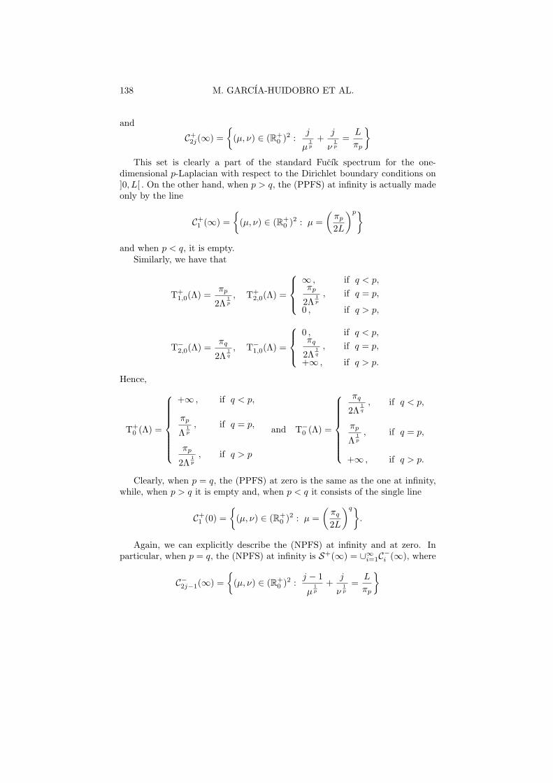
138 M. GARCIA-HUIDOBRO ET AL.
and
C+2j(∞) =
{
(µ, ν) ∈ (R+0 )
2 :j
µ1p
+j
ν1p
=L
πp
}
This set is clearly a part of the standard Fucık spectrum for the one-dimensional p-Laplacian with respect to the Dirichlet boundary conditions on]0, L[ . On the other hand, when p > q, the (PPFS) at infinity is actually madeonly by the line
C+1 (∞) =
{
(µ, ν) ∈ (R+0 )
2 : µ =
(
πp2L
)p}
and when p < q, it is empty.Similarly, we have that
T+1,0(Λ) =
πp
2Λ1p
, T+2,0(Λ) =
∞ , if q < p,πp
2Λ1p
, if q = p,
0 , if q > p,
T−2,0(Λ) =
πq
2Λ1q
, T−1,0(Λ) =
0 , if q < p,πq
2Λ1q
, if q = p,
+∞ , if q > p.
Hence,
T+0 (Λ) =
+∞ , if q < p,
πp
Λ1p
, if q = p,
πp
2Λ1p
, if q > p
and T−0 (Λ) =
πq
2Λ1q
, if q < p,
πp
Λ1p
, if q = p,
+∞ , if q > p.
Clearly, when p = q, the (PPFS) at zero is the same as the one at infinity,while, when p > q it is empty and, when p < q it consists of the single line
C+1 (0) =
{
(µ, ν) ∈ (R+0 )
2 : µ =
(
πq2L
)q}
.
Again, we can explicitly describe the (NPFS) at infinity and at zero. Inparticular, when p = q, the (NPFS) at infinity is S+(∞) = ∪∞
i=1C−i (∞), where
C−2j−1(∞) =
{
(µ, ν) ∈ (R+0 )
2 :j − 1
µ1p
+j
ν1p
=L
πp
}

FUCIK SPECTRUM AND NUMBER OF SOLUTION 139
and
C−2j(∞) =
{
(µ, ν) ∈ (R+0 )
2 :j
µ1p
+j
ν1p
=L
πp
}
.
To show the role of the strong asymmetry when p 6= q for the map φ defined
in (8), we consider f satisfying (f1) and assume that f(s)φ(s) → a± as s→ 0± and
f(s)φ(s) → A± as s→ ±∞, for some positive constants a± and A±. Then, if p > q,
it follows that problem (P ) has at least one solution with positive slope at t = 0if A+ >
( πp
2L
)pand it has at least one solution with negative slope at t = 0
if a− >( πq
2L
)q.
We remark that, according to [20], the same spectra at infinity (or, respec-tively, at zero) is obtained, and therefore, the same application to problem (P )will occur for any function φ having the form of
φ(s) =
{
ψ1(s), for s ≥ 0,
ψ2(s), for s ≤ 0,
where ψ1 : R+ → R
+ and ψ2 : R− → R
− are increasing bijections withψi(0) = 0 and
lims→+∞, 0+
ψ1(σs)
ψ1(s)= σp−1, for allσ > 0,
and
lims→−∞, 0−
ψ2(σs)
ψ2(s)= σq−1, for allσ > 0,
for some p, q > 1.
Example 2. Continuing along this direction, we could consider (like it wasdone in [20] for an odd φ), the case of a φ-function such that for some p, q > 1,
lims→±∞
φ(σs)
φ(s)= σp−1, for allσ > 0, (9)
and
lims→0±
φ(σs)
φ(s)= σq−1, for allσ > 0. (10)
Hence, we have a (PPFS) and also a (NPFS) at infinity and one at zero, whichare the same like those for the p-Laplacian and the q-Laplacian, respectively.Observe that here we do not assume the φ to be odd. For instance, a map ofthe form
φ : s 7→
φp(s), s ≤ −1,
φq(s), −1 ≤ s ≤ 0,
log(1 + sq−1), 0 ≤ s ≤ 1,
φp(s) log(1 + s), s ≥ 1,

140 M. GARCIA-HUIDOBRO ET AL.
is suitable for our applications.As a consequence of Theorem 2.1, we have the following
Corollary 4.1. Let φ satisfy (φ1), (9), and (10). Suppose that there arepositive numbers a+, a−, A+, A− such that
lims→0+
f(s)
φ(s)= a+, lim
s→0−
f(s)
φ(s)= a−
and
lims→+∞
f(s)
φ(s)= A+, lim
s→−∞
f(s)
φ(s)= A−.
Assume also that there are k, ℓ ∈ N with k 6= ℓ such that, for k = 2j
j
(a+)1q
+j − 1
(a−)1q
<L
πq<
j
(a+)1q
+j
(a−)1q
and for k = 2j + 1
j
(a+)1q
+j
(a−)1q
<L
πq<
j + 1
(a+)1q
+j
(a−)1q
while, for ℓ = 2i,
i
(A+)1p
+i− 1
(A−)1p
<L
πp<
i
(A+)1p
+i
(A−)1p
and for ℓ = 2i+ 1,
i
(A+)1p
+i
(A−)1p
<L
πp<
i+ 1
(A+)1p
+i
(A−)1p
Then, problem (P ) has at least |k − ℓ| solutions with u′(0) > 0.
Clearly, a symmetric result holds for the (NPFS).To show an application of Corollary 4.1 which resembles the one given in
the Introduction (this time for q = 2), we consider the following situation.
Example 3. Let φ : R → R be an increasing bijection which is of class C1
in a neighborhood of zero, with φ′(0) > 0 and satisfies (9) for some p > 1.Suppose also that we have
lims→0+
f(s)
φ(s)= lim
s→+∞
f(s)
φ(s)= a
lims→0−
f(s)
φ(s)= lim
s→−∞
f(s)
φ(s)= b
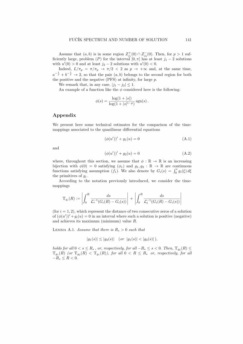
FUCIK SPECTRUM AND NUMBER OF SOLUTION 141
Assume that (a, b) is in some region Z+j1(0) ∩ Z−
j2(0). Then, for p > 1 suf-
ficiently large, problem (P ) for the interval [0, π] has at least j1 − 2 solutionswith u′(0) > 0 and at least j2 − 2 solutions with u′(0) < 0.
Indeed, L/πp = π/πp → π/2 < 2 as p → +∞ and, at the same time,
a−1p + b−
1p → 2, so that the pair (a, b) belongs to the second region for both
the positive and the negative (PFS) at infinity, for large p.We remark that, in any case, |j1 − j2| ≤ 1.An example of a function like the φ considered here is the following:
φ(s) =log(1 + |s|)
log(1 + |s|1−p)sgn(s) .
Appendix
We present here some technical estimates for the comparison of the time-mappings associated to the quasilinear differential equations
(φ(u′))′ + g1(u) = 0 (A.1)
and
(φ(u′))′ + g2(u) = 0 (A.2)
where, throughout this section, we assume that φ : R → R is an increasingbijection with φ(0) = 0 satisfying (φ1) and g1, g2 : R → R are continuousfunctions satisfying assumption (f1). We also denote by Gi(s) =
∫ s
0gi(ξ) dξ
the primitives of gi .According to the notation previously introduced, we consider the time-
mappings
Tgi(R) :=
∣
∣
∣
∣
∣
∫ R
0
ds
L−1r (Gi(R)−Gi(s))
∣
∣
∣
∣
∣
+
∣
∣
∣
∣
∣
∫ R
0
ds
L−1l (Gi(R)−Gi(s))
∣
∣
∣
∣
∣
(for i = 1, 2), which represent the distance of two consecutive zeros of a solutionof (φ(u′))′+gi(u) = 0 in an interval where such a solution is positive (negative)and achieves its maximum (minimum) value R.
Lemma A.1. Assume that there is R∗ > 0 such that
|g1(s)| ≤ |g2(s)| (or |g1(s)| < |g2(s)| ),
holds for all 0 < s ≤ R∗ , or, respectively, for all −R∗ ≤ s < 0. Then, Tg2(R) ≤Tg1(R) (or Tg2(R) < Tg1(R)), for all 0 < R ≤ R∗ or, respectively, for all−R∗ ≤ R < 0.

142 M. GARCIA-HUIDOBRO ET AL.
Proof. We consider only the case when R > 0, being the other one completelysymmetric. Then, by the assumption, given any R ∈ ]0, R∗], we have thatg1(s) ≤ g2(s) (or g1(s) < g2(s)) for all s ∈ ]0, R]. Hence,
G1(R)−G1(s) =
∫ R
s
g1(ξ) dξ ≤
∫ R
s
g2(ξ) dξ = G2(R)−G2(s)
(or G1(R)−G1(s) < G2(R)−G2(s)) holds for each 0 < s ≤ R. From this andthe definition of Tgi(R), the result immediately follows.
Lemma A.2. Assume that there is R∗ > 0 such that
|g1(s)| ≤ |g2(s)|,
holds for all s ≥ R∗ , or, respectively, for all s ≤ −R∗. Then, for each ε > 0there is Rε > R∗ such that
Tg2(R) ≤ Tg1(R) + ε
holds for all R > Rε , or, respectively, for all R < −Rε .
Proof. As before, we discuss only the case when R > 0. Let ui be the solution of(φ(u′))′+ gi(u) = 0, for i = 1, 2, with ui(0) = 0 and maxui = u(t∗i ) = R > R∗ .From the equation, we see that ui is strictly increasing in [0, t∗i ] and strictlydecreasing in [t∗i ,Tg1(R)]. Hence there are uniquely determined t−i and t+i , with0 < t−i < t∗i < t+i < Tg1(R), such that ui(t) ≥ R∗ for t ∈ [0,Tg1(R)] if andonly if t ∈ [t−i , t
+i ]. By the same argument like in the proof of Lemma A.1, it
easily follows that∫ R
R∗
ds
L−1r (G2(R)−G2(s))
+
∫ R
R∗
ds
|L−1l (G2(R)−G2(s))|
≤
∫ R
R∗
ds
L−1r (G1(R)−G1(s))
+
∫ R
R∗
ds
|L−1l (G1(R)−G1(s))|
.
Therefore, we have that
Tg2(R)− Tg1(R)
≤∑
i=1,2
((t+i − t∗) + (t∗ − t−i ))
=∑
i=1,2
(
∫ R∗
0
ds
L−1r (Gi(R)−Gi(s))
+
∫ R∗
0
ds
|L−1l (Gi(R)−Gi(s))|
)
≤∑
i=1,2
(
R∗
L−1r (Gi(R)−Gi(R∗))
+R∗
|L−1l (Gi(R)−Gi(s))|
)
holds for each R > R∗. At this point, the result easily follows, using (f1) andletting R→ +∞.

FUCIK SPECTRUM AND NUMBER OF SOLUTION 143
The next result is a straightforward consequence of Lemma A.2
Corollary A.1. Assume that there is R∗ > 0 such that
|g1(s)| ≤ |g2(s)|,
holds for all s ≥ R∗ , or, respectively, for all s ≤ −R∗. Then
lim supR→+∞
Tg2(R) ≤ lim infR→+∞
Tg1(R)
(respectively, lim supR→−∞ Tg2(R) ≤ lim infR→−∞ Tg1(R)).
References
[1] M. Abramowitz and I. Stegun, Handbook of mathematical functions, Dover,New York (1965).
[2] L. Boccardo, P. Drabek, D. Giachetti and M. Kucera, Generalization
of Fredholm alternative for nonlinear differential operators, Nonlinear Anal. 10(1986), 1083–1103.
[3] A. Capietto, An existence result for a two-point superlinear boundary value
problem, Proceedings of the 2nd International Conference on Differential Equa-tions, Marrakesh (1995).
[4] A. Capietto and W. Dambrosio, Multiplicity results for some two-point super-
linear asymmetric boundary value problem, Nonlinear Anal. 38 (1999), 869–896.
[5] A. Capietto and W. Dambrosio, Boundary value problems with sublinear
conditions near zero, NoDEA Nonlinear Differential Equations Appl. 6 (1999),149–172.
[6] A. Capietto, J. Mawhin and F. Zanolin, Boundary value problems for forced
superlinear second order ordinary differential equations, in H. Brezis, Nonlinear
partial differential equations and their applications, Taylor & Francis (1994).
[7] A. Capietto, J. Mawhin and F. Zanolin, On the existence of two solutions
with a prescribed number of zeros for a superlinear two-point boundary value
problem, Topol. Methods Nonlinear Anal. 6 (1995), 175–188.
[8] W. Dambrosio, Time-map techniques for some boundary value problems, RockyMountain J. Math. 28 (1998), 885–926.
[9] W. Dambrosio, Multiple solutions of weakly-coupled systems with p-Laplacian
operators, Results Math. 36 (1998), 34–54.
[10] M. Del Pino, M. Elgueta and R. Manasevich, A homotopic deformation
along p of a Leray-Schauder degree result and existence for (|u′|p−2u′)′+f(t, u) =0, u(0) = u(T ) = 0, p > 1, J. Differential Equations 80 (1992), 1–13.
[11] M.A. Del Pino, R.F. Manasevich and A.E. Murua, Existence and multi-
plicity of solutions with prescribed period for a second order quasilinear ODE,Nonlinear Anal. 18 (1992), 79–92.
144 M. GARCIA-HUIDOBRO ET AL.
[12] G. Dinca and L. Sanchez, Multiple solutions of boundary value problems: an
elementary approach via the shooting method, NoDEA Nonlinear DifferentialEquations Appl. 1 (1994), 163–178.
[13] P. Drabek, Solvability of boundary value problems with homogeneous ordinary
differential operator, Rend. Istit. Mat. Univ. Trieste 18 (1986), 105–124.
[14] P. Drabek and R. Manasevich, On the closed solution to some nonhomoge-
neous eigenvalue problems with p-Laplacian, Differential Integral Equations 12
(1999), 773–788.
[15] S. Fucık, Solvability of nonlinear equations and boundary value problems, Rei-del, Dordrecht (1980).
[16] M. Garcıa-Huidobro, R. Manasevich and F. Zanolin, Strongly nonlinear
second order ODE’s with unilateral conditions, Differential Integral Equations 6(1993), 1057–1078.
[17] M. Garcıa-Huidobro, R. Manasevich and F. Zanolin, A Fredholm-like
result for strongly nonlinear second order ODE’s, J. Differential Equations 114
(1994), 132–167.
[18] M. Garcıa-Huidobro, R. Manasevich and F. Zanolin, On a pseudo Fucık
spectrum for strongly nonlinear second order ODE’s and an existence result, J.Comput. Appl. Math. 52 (1994), 219–239.
[19] M. Garcıa-Huidobro, R. Manasevich and F. Zanolin, Infinitely many so-
lutions for a Dirichlet problem with a nonhomogeneous p-Laplacian-like operator
in a ball, Adv. Differential Equations 2 (1997), 203–230.
[20] M. Garcıa-Huidobro and P. Ubilla, Multiplicity of solutions for a class of
second-order equations, Nonlinear Anal. 28 (1997), 1509–1520.
[21] P. Habets, M. Ramos and L. Sanchez, Jumping nonlinearities for Neumann
BVPs with positive forcing, Nonlinear Anal. 20 (1993), 533–549.
[22] M. Henrard, Infinitely many solutions of weakly coupled superlinear systems,Adv. Differential Equations 2 (1997), 753–778.
[23] R. Manasevich and F. Zanolin, Time-mappings and multiplicity of solutions
for the one-dimensional p-Laplacian, Nonlinear Anal. 21 (1993), 269–291.
[24] Z. Opial, Sur les periodes des solutiones de l’equation differentielle x′′+g(x) =0, Ann. Polon. Math. 10 (1961), 49–72.
[25] C. Rebelo, A note on uniqueness of Cauchy problems associated to planar
Hamiltonian systems, Portugal. Math. 57 (2000), 415–419.
Authors’ addresses:
Marta Garcıa-Huidobro
Departamento de Matematicas
P. Universidad Catolica de Chile
Casilla 306, Correo 22, Santiago, Chile
E-mail: [email protected]

FUCIK SPECTRUM AND NUMBER OF SOLUTION 145
Raul Manasevich
Centro de Modelamiento Matematico and Departamento de Ingenierıa Matematica
Universidad de Chile
Casilla 170, Correo 3, Santiago, Chile
E-mail: [email protected]
Fabio Zanolin
Dipartimento di Matematica e Informatica
Universita di Udine
Via delle Scienze 206, 33100 Udine, Italy
E-mail: [email protected]
Received November 16, 2011


![Improved Distributed Degree Splitting and Edge Coloringdegree splitting requires (logn) rounds, as shown by Chang et al. [6], and randomized degree splitting requires (loglogn) rounds,](https://static.fdocument.pub/doc/165x107/60d017d83325af5de42c2850/improved-distributed-degree-splitting-and-edge-coloring-degree-splitting-requires.jpg)