Solving Underdetermined Linear Equations and ...rom-gr/slides/Justin_Romberg.pdf · Solving...
69
Solving Underdetermined Linear Equations and Overdetermined Quadratic Equations (using Convex Programming) Justin Romberg Georgia Tech, ECE Caltech ROM-GR Workshop June 7, 2013 Pasadena, California
Transcript of Solving Underdetermined Linear Equations and ...rom-gr/slides/Justin_Romberg.pdf · Solving...
Solving Underdetermined Linear Equations andOverdetermined Quadratic Equations
(using Convex Programming)
Justin RombergGeorgia Tech, ECE
Caltech ROM-GR WorkshopJune 7, 2013
Pasadena, California
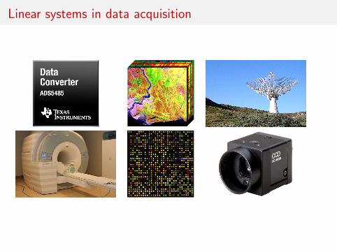
Linear systems in data acquisition

Linear systems of equations are ubiquitous
Model:
y
=
A
x
y: data coming off of sensorA: mathematical (linear) model for sensorx: signal/image to reconstruct

Classical: When can we stably “invert” a matrix?
Suppose we have an M ×N observation matrix A with M ≥ N(MORE observations than unknowns), through which we observe
y = Ax0 + noise
Standard way to recover x0, use the pseudo-inverse
solve minx‖y −Ax‖22 ⇔ x = (ATA)−1AT y
Q: When is this recovery stable? That is, when is
‖x− x0‖22 ∼ ‖noise‖22 ?
A: When the matrix A preserves distances ...
‖A(x1 − x2)‖22 ≈ ‖x1 − x2‖22 for all x1, x2 ∈ RN
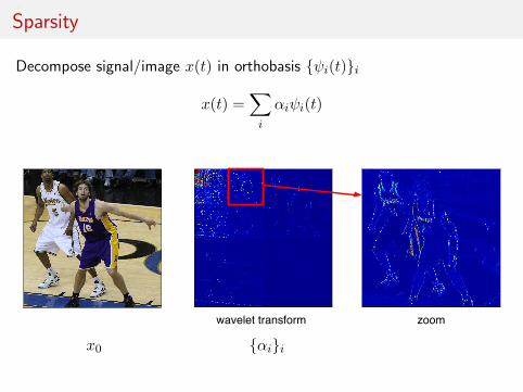
Sparsity
Decompose signal/image x(t) in orthobasis {ψi(t)}i
x(t) =∑
i
αiψi(t)
wavelet transform zoom
x0 {αi}i

Wavelet approximation
Take 1% of largest coefficients, set the rest to zero (adaptive)
original approximated
rel. error = 0.031
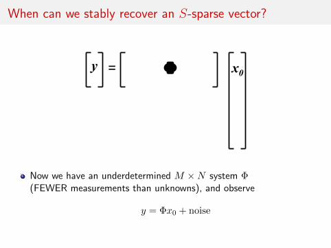
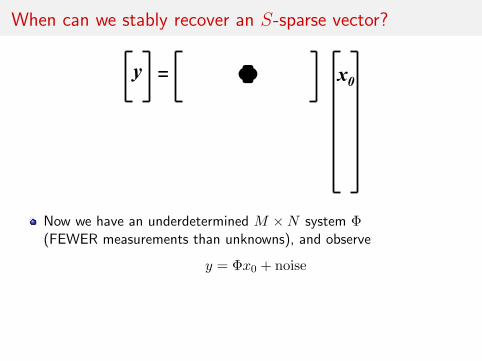
When can we stably recover an S-sparse vector?
y ! x0=
Now we have an underdetermined M ×N system Φ(FEWER measurements than unknowns), and observe
y = Φx0 + noise
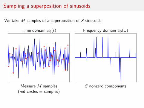
Sampling a superposition of sinusoids
We take M samples of a superposition of S sinusoids:
Time domain x0(t) Frequency domain x0(ω)
Measure M samples S nonzero components(red circles = samples)

Sampling a superposition of sinusoids
Reconstruct by solving
minx‖x‖`1 subject to x(tm) = x0(tm), m = 1, . . . ,M
original x0, S = 15 perfect recovery from 30 samples

Numerical recovery curves
Resolutions N = 256, 512, 1024 (black, blue, red)
Signal composed of S randomly selected sinusoids
Sample at M randomly selected locations
% success
0 0.2 0.4 0.6 0.8 10
10
20
30
40
50
60
70
80
90
100
S/M
In practice, perfect recovery occurs when M ≈ 2S for N ≈ 1000

A nonlinear sampling theorem
Exact Recovery Theorem (Candes, R, Tao, 2004):
Unknown x0 is supported on set of size S
Select M sample locations {tm} “at random” with
M ≥ Const · S logN
Take time-domain samples (measurements) ym = x0(tm)
Solve
minx‖x‖`1 subject to x(tm) = ym, m = 1, . . . ,M
Solution is exactly f with extremely high probability
When can we stably recover an S-sparse vector?
y ! x0=
Now we have an underdetermined M ×N system Φ(FEWER measurements than unknowns), and observe
y = Φx0 + noise
We can recover x0 when Φ keeps sparse signals separated
‖Φ(x1 − x2)‖22 ≈ ‖x1 − x2‖22for all S-sparse x1, x2

When can we stably recover an S-sparse vector?
Now we have an underdetermined M ×N system Φ(FEWER measurements than unknowns), and observe
y = Φx0 + noise
We can recover x0 when Φ keeps sparse signals separated
‖Φ(x1 − x2)‖22 ≈ ‖x1 − x2‖22
for all S-sparse x1, x2

When can we stably recover an S-sparse vector?
Now we have an underdetermined M ×N system Φ(FEWER measurements than unknowns), and observe
y = Φx0 + noise
We can recover x0 when Φ keeps sparse signals separated
‖Φ(x1 − x2)‖22 ≈ ‖x1 − x2‖22for all S-sparse x1, x2
To recover x0, we solve
minx‖x‖0 subject to Φx = y
‖x‖0 = number of nonzero terms in x
This program is computationally intractable

When can we stably recover an S-sparse vector?
Now we have an underdetermined M ×N system Φ(FEWER measurements than unknowns), and observe
y = Φx0 + noise
We can recover x0 when Φ keeps sparse signals separated
‖Φ(x1 − x2)‖22 ≈ ‖x1 − x2‖22for all S-sparse x1, x2
A relaxed (convex) program
minx‖x‖1 subject to Φx = y
‖x‖1 =∑
k |xk|
This program is very tractable (linear program)
The convex program can recover nearly all “identifiable” sparsevectors, and it is robust.

Intuition for `1
minx ‖x‖2 s.t. Φx = y minx ‖x‖1 s.t. Φx = y!"#$L2 %&'()*+$!&,-$
.'/(+$(01/,'(234)4313$L5 (&.1+4&)4($/.3&(+$never sparse
!"#$L1 !%&'(
)*+*),)$L1 (%-,.*%+/$L0 (01&(2(.$(%-,.*%+$*3
random orientationdimension N-M
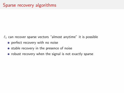
Sparse recovery algorithms
`1 can recover sparse vectors “almost anytime” it is possible
perfect recovery with no noise
stable recovery in the presence of noise
robust recovery when the signal is not exactly sparse

Sparse recovery algorithms
Other recovery techniques have similar theoretical properties(their practical effectiveness varies with applications)
greedy algorithms
iterative thresholding
belief propagation
specialized decoding algorithms
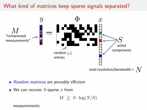
What kind of matrices keep sparse signals separated?
Φ
!"#$%&&"'()'*%*+,&
S
-!*.'(&%*+-/%,&
±1
0"'()-%,,%.&(%!,1-%(%*+,2&
M
N+'+!3&-%,'31#'*45!*.6/.+7&8&
Random matrices are provably efficient
We can recover S-sparse x from
M & S · log(N/S)
measurements
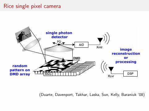
Rice single pixel cameraRice Single-Pixel CS Camera
randompattern onDMD array
DMD DMD
single photon detector
imagereconstruction
orprocessing
(Duarte, Davenport, Takhar, Laska, Sun, Kelly, Baraniuk ’08)
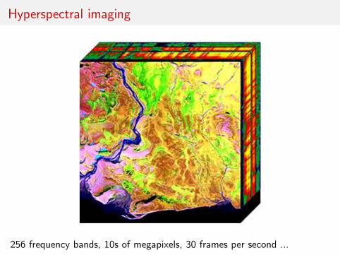
Hyperspectral imaging
256 frequency bands, 10s of megapixels, 30 frames per second ...
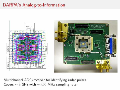
DARPA’s Analog-to-Information
Multichannel ADC/receiver for identifying radar pulsesCovers ∼ 3 GHz with ∼ 400 MHz sampling rate

Compressive sensing with structured randomness
Subsampled rows of “incoherent” orthogonal matrix
Can recover S-sparse x0 with
M & S logaN
measurements
Candes, R, Tao, Rudelson, Vershynin, Tropp, . . .

Accelerated MRISPIR-iT with Wavelet CS
ARC SPIR-iT
(Lustig et al. ’08)

Matrices for sparse recovery with structured randomness
Random convolution + subsampling
Universal; Can recover S-sparse x0 with
M & S logaN
Applications include:
radar imaging
sonar imaging
seismic exploration
channel estimation for communications
super-resolved imaging
R, Bajwa, Haupt, Tropp, Rauhut, . . .

Integrating compression and sensing
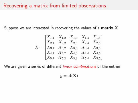
Recovering a matrix from limited observations
Suppose we are interested in recovering the values of a matrix X
X =
X1,1 X1,2 X1,3 X1,4 X1,5
X2,1 X2,2 X2,3 X2,4 X2,5
X3,1 X3,2 X3,3 X3,4 X3,5
X4,1 X4,2 X4,3 X4,4 X4,5
X5,1 X5,2 X5,3 X5,4 X5,5
We are given a series of different linear combinations of the entries
y = A(X)

Example: matrix completion
Suppose we do not see all the entries in a matrix ...
X =
X1,1 − X1,3 − X1,5
− X2,2 − X2,4 −− X3,2 X3,3 − −X4,1 − − X4,4 X4,5
− − − X5,4 X5,5
... can we “fill in the blanks”?
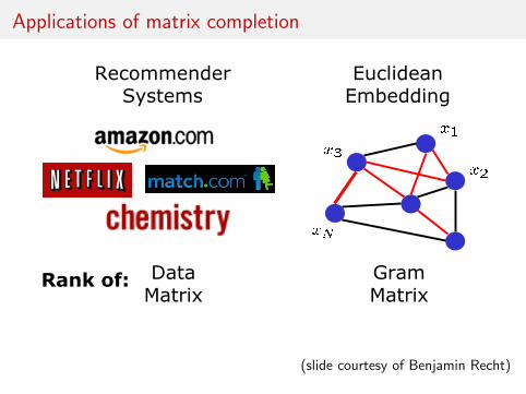
Applications of matrix completion
G
K
ControllerDesign
Constraints involving the rank of the Hankel Operator, Matrix, or Singular Values
Model Reduction
SystemIdentification
Multitask Learning
EuclideanEmbedding
Rank of: Matrix of Classifiers
GramMatrix
RecommenderSystems
DataMatrix
(slide courtesy of Benjamin Recht)

Low rank structure
2666666664
X
3777777775
=
2666666664
L
3777777775
24 RT
35
K ⇥ N K ⇥ R
R ⇥ N
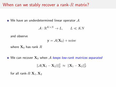
When can we stably recover a rank-R matrix?
We have an underdetermined linear operator A
A : RK×N → L, L� KN
and observey = A(X0) + noise
where X0 has rank R
We can recover X0 when A keeps low-rank matrices separated
‖A(X1 −X2)‖22 ≈ ‖X1 −X2‖2F
for all rank-R X1,X2
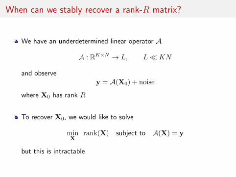
When can we stably recover a rank-R matrix?
We have an underdetermined linear operator A
A : RK×N → L, L� KN
and observey = A(X0) + noise
where X0 has rank R
To recover X0, we would like to solve
minX
rank(X) subject to A(X) = y
but this is intractable

When can we stably recover a rank-R matrix?
We have an underdetermined linear operator A
A : RK×N → L, L� KN
and observey = A(X0) + noise
where X0 has rank R
A relaxed (convex) program
minX‖X‖∗ subject to A(X) = y
where ‖X‖∗ = sum of the singular values of X
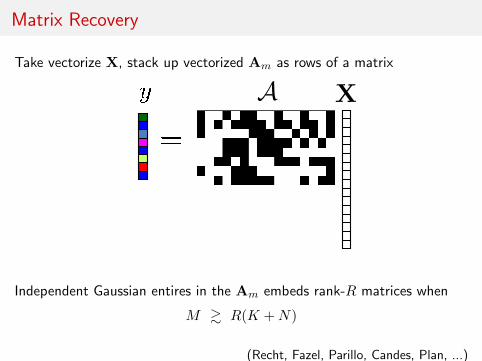
Matrix Recovery
Take vectorize X, stack up vectorized Am as rows of a matrix
A X
Independent Gaussian entires in the Am embeds rank-R matrices when
M & R(K +N)
(Recht, Fazel, Parillo, Candes, Plan, ...)

Example: matrix completion
Suppose we do not see all the entries in a matrix ...
X =
X1,1 − X1,3 − X1,5
− X2,2 − X2,4 −− X3,2 X3,3 − −X4,1 − − X4,4 X4,5
− − − X5,4 X5,5
... we can fill them in from
M & R(K +N) log2(KN)
randomly chosen samples if X is diffuse.
(Recht, Candes, Tao, Montenari, Oh, ...)
Summary: random projections and structured recovery
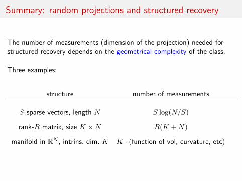
The number of measurements (dimension of the projection) needed forstructured recovery depends on the geometrical complexity of the class.
Three examples:
structure number of measurements
S-sparse vectors, length N S log(N/S)
rank-R matrix, size K ×N R(K +N)
manifold in RN , intrins. dim. K K · (function of vol, curvature, etc)

Systems of quadratic and bilinear equations

Quadratic equations
Quadratic equations contain unknown terms multiplied by one another
x1x3 + x2 + x25 = 13
3x2x6 − 7x3 + 9x24 = −12
...
Their nonlinearity makes them trickier to solve, and the computationalframework is nowhere nearly as strong as for linear equations
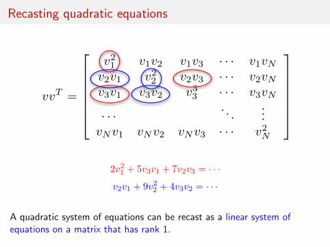
Recasting quadratic equations
vvT =
2666664
v21 v1v2 v1v3 · · · v1vN
v2v1 v22 v2v3 · · · v2vN
v3v1 v3v2 v33 · · · v3vN
· · · . . ....
vNv1 vNv2 vNv3 · · · v2N
3777775
2v21 + 5v3v1 + 7v2v3 = · · ·v2v1 + 9v22 + 4v3v2 = · · ·
A quadratic system of equations can be recast as a linear system ofequations on a matrix that has rank 1.

Recasting quadratic equations
vvT =
2666664
v21 v1v2 v1v3 · · · v1vN
v2v1 v22 v2v3 · · · v2vN
v3v1 v3v2 v33 · · · v3vN
· · · . . ....
vNv1 vNv2 vNv3 · · · v2N
3777775
Compressive (low rank) recovery ⇒“Generic” quadratic systems with cN equations and N unknowns can besolved using nuclear norm minimization

Blind deconvolution
image deblurring multipath in wireless comm
We observey[n] =
∑
`
w[`]x[n− `]
and want to “untangle” w and x.
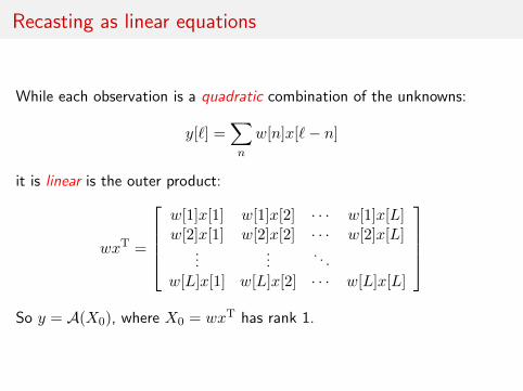
Recasting as linear equations
While each observation is a quadratic combination of the unknowns:
y[`] =∑
n
w[n]x[`− n]
it is linear is the outer product:
wxT =
w[1]x[1] w[1]x[2] · · · w[1]x[L]w[2]x[1] w[2]x[2] · · · w[2]x[L]
......
. . .
w[L]x[1] w[L]x[2] · · · w[L]x[L]
So y = A(X0), where X0 = wxT has rank 1.
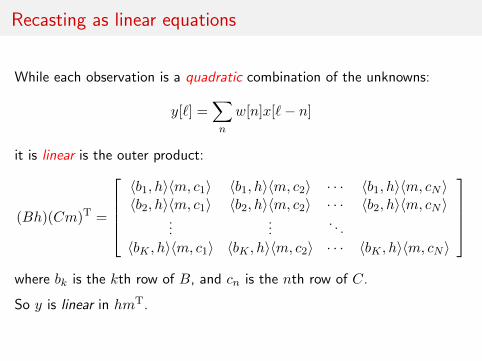
Recasting as linear equations
While each observation is a quadratic combination of the unknowns:
y[`] =∑
n
w[n]x[`− n]
it is linear is the outer product:
(Bh)(Cm)T =
〈b1, h〉〈m, c1〉 〈b1, h〉〈m, c2〉 · · · 〈b1, h〉〈m, cN 〉〈b2, h〉〈m, c1〉 〈b2, h〉〈m, c2〉 · · · 〈b2, h〉〈m, cN 〉
......
. . .
〈bK , h〉〈m, c1〉 〈bK , h〉〈m, c2〉 · · · 〈bK , h〉〈m, cN 〉
where bk is the kth row of B, and cn is the nth row of C.
So y is linear in hmT.

Blind deconvolution theoretical results
We observe
y = w ∗ x, w = Bh, x = Cm
= A(hm∗), h ∈ RK , m ∈ RN ,
and then solve
minX‖X‖∗ subject to A(X) = y.
Ahmed, Recht, R, ’12:If B is “incoherent” in the Fourier domain, and C is randomly chosen,then we will recover X0 = hm∗ exactly (with high probability) when
max(K,N) ≤ L
log3 L

Numerical results
white = 100% success, black = 0% success
w sparse, x sparse w sparse, x short
We can take K +N ≈ L/3

Numerical results
Unknown image with known support in the wavelet domain,Unknown blurring kernel with known support in spatial domain
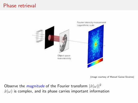
Phase retrieval
(image courtesy of Manuel Guizar-Sicairos)
Observe the magnitude of the Fourier transform |x(ω)|2x(ω) is complex, and its phase carries important information

Phase retrieval
(image courtesy of Manuel Guizar-Sicairos)
Recently, Candes, Strohmer, Voroninski, have looked at stylized version ofphase retrieval:
observe y` = |〈a`,x〉|2 ` = 1, . . . , L
and shown that x ∈ RN can be recovered when L ∼ Const ·Nfor random a`.

Random projections in fast forward modeling
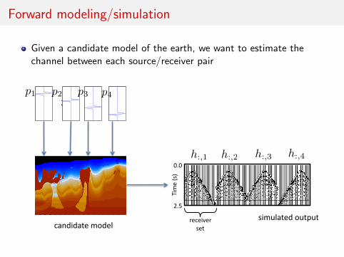
Forward modeling/simulation
Given a candidate model of the earth, we want to estimate thechannel between each source/receiver pair
!"
#$#"
%$&"
'()*"+,-"
""!""""""""""%""""""""""".""""""""""/"
0*1*(2*0",*3"
h:,4h:,3h:,2h:,1
p1 p4p3p2
1456(643*")76*8",()9843*6"793:93"
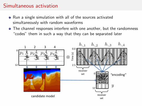
Simultaneous activation
Run a single simulation with all of the sources activatedsimultaneously with random waveforms
The channel responses interfere with one another, but the randomness“codes” them in such a way that they can be separated later
!"
#$#"
%$&"
'()*"+,-"
""!""""""""""%""""""""""".""""""""""/"
#"
!%"
#"
!%"
!
0*1*(2*0",*3"
0*1*(2*0",*3"
h:,4h:,3h:,2h:,1
p1 p2 p3 p4
y
4*5167(589"
1:57(7:3*")67*;"

Multiple channel linear algebra
G1 G2 · · · Gp
...
=ykh1,k
h2,k !"#$$%&'()*((
&%$+,"((n
!)$-)&./)$(01,"(2.&'%( pj
m
hc,k
How long does each pulse need to be to recover all of the channels?(the system is m× nc, m = pulse length, c =# channels)
Of course we can do it for m ≥ ncBut if the channels have a combined sparsity of S, then we can takem ∼ s+ n
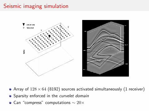
Seismic imaging simulation
Figure 1: Source and receiver geometry. We use 8192 (128 ! 64) sources and 1 receiver.
33
(a) Simple case. (b) More complex case.
Figure 2: Desired band-limited Greens’s functions obtained by sequential-source modeling:(a) Simple case and (b) More complex case.
34
Array of 128× 64 (8192) sources activated simultaneously (1 receiver)
Sparsity enforced in the curvelet domain
Can “compress” computations ∼ 20×
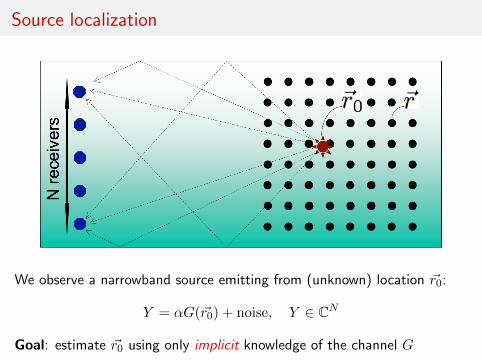
Source localization
We observe a narrowband source emitting from (unknown) location ~r0:
Y = αG(~r0) + noise, Y ∈ CN
Goal: estimate ~r0 using only implicit knowledge of the channel G

Matched field processing
|〈Y,G(~r)〉|2
!
!
"#$$ "%$$ "&$$ "'$$ &$$$
"$
($$
("$
!#$
!("
!($
!"
$
Given observations Y , estimate ~r0 by “matching against the field”:
r = arg min~r
minβ∈C‖Y − βG(~r)‖2 = max
~r
|〈Y,G(~r)〉|2‖G(~r)‖2 ≈ |〈Y,G(~r)〉|2
We do not have direct access to G, but can calculate 〈Y,G(~r)〉 for all ~rusing time-reversal

Multiple realizations
We receive a series of measurements Y1, . . . , YK from the sameenvironment (but possibly different source locations)
Calculating GHYk for each instance can be expensive(requires a PDE solve)
A naıve precomputing approach:I set off a source at each receiver location ~siI time reverse GH1~si to “pick off” a row of G
We can use ideas from compressive sensing to significantly reduce theamount of precomputation

Coded simulations
Pre-compute the responses to a series of randomly and simultaneouslyactivated sources along the receiver array
b1 = GHφ1, b2 = GHφ2, . . . bM = GHφM ,
where the φm are random vectors
Stack up the bHm to form the matrix ΦG
Given the observations Y , code them to form ΦY , and solve
rcs = arg min~r
minβ∈C‖ΦY − βΦG(~r)‖22 = arg max
~r
|〈ΦY,ΦG(~r)〉|2‖ΦG(~r)‖2
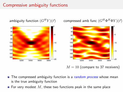
Compressive ambiguity functions
ambiguity function (GHY )(~r) compressed amb func (GHΦHΦY )(~r)
"200 "400 "600 "800
20
40
60
80
100
120
140
160
180!20
!1"
!10
!"
0
"200 "400 "600 "800
20
40
60
80
100
120
140
160
180!20
!1"
!10
!"
0
M = 10 (compare to 37 receivers)
The compressed ambiguity function is a random process whose meanis the true ambiguity function
For very modest M , these two functions peak in the same place
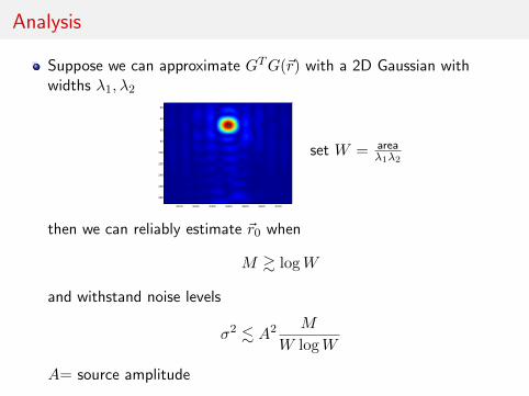
Analysis
Suppose we can approximate GTG(~r) with a 2D Gaussian withwidths λ1, λ2
5100 5200 5300 5400 5500 5600 5700
20
40
60
80
100
120
140
160
180
set W = areaλ1λ2
then we can reliably estimate ~r0 when
M & logW
and withstand noise levels
σ2 . A2 M
W logW
A= source amplitude
Sampling ensembles of correlated signals

Sensor arrays

Neural probes
!!!!!!!!"""
!!!!!!!!"""
!"#$%&
$'%&
#'(%&
)"%&
recording site
Up to 100s of channels sampled at ∼ 100 kHz
10s of millions of samples/second
Near Future: 1 million channels, terabits per second

Correlated signals
M
Nyquist acquisition:
sampling rate ≈ (number of signals)× (bandwith)
= M ·W
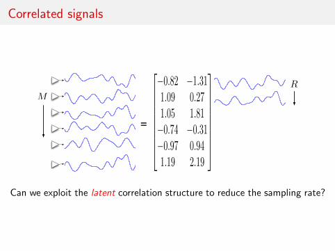
Correlated signals
−0.82 −1.311.09 0.271.05 1.81−0.74 −0.31−0.97 0.941.19 2.19
=
M
R
Can we exploit the latent correlation structure to reduce the sampling rate?
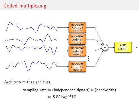
Coded multiplexing
modulator
modulator
modulator
modulator
+
...
ADC
code p1rate ϕ
code p2
code p3
rate ϕ
rate ϕ
rate ϕ
rate ϕ
...code pM
y
Architecture that achieves
sampling rate ≈ (independent signals)× (bandwidth)
≈ RW log3/2W

References
E. Candes, J. Romberg, T. Tao, “Stable Signal Recovery from Incomplete and Inaccurate Measurements,” CPAM, 2006.
E. Candes and J. Romberg, “Sparsity and Incoherence in Compressive Sampling,” Inverse Problems, 2007.
J. Romberg, “Compressive Sensing by Random Convolution,” SIAM J. Imaging Science, 2009.
A. Ahmed, B. Recht, and J. Romberg, “Blind Deconvolution using Convex Programming,” submitted to IEEETransactions on Information Theory, November 2012.
A. Ahmed and J. Romberg, “Compressive Sampling of Correlated Signals,” Manuscript in preparation.Preliminary version at IEEE Asilomar Conference on Signals, Systems, and Computers, October 2011.
A. Ahmed and J. Romberg, “Compressive Multiplexers for Correlated Signals,” Manuscript in preparation.Preliminary version at IEEE Asilomar Conference on Signals, Systems, and Computers, November 2012.
http://users.ece.gatech.edu/~justin/Publications.html