
Simulation and Real-Time Analysis of Pulse Shapes from ...The nucleus is a strongly-interacting many...
171
Fakult¨atf¨ ur Physik der Technischen Universit¨at M¨ unchen Physik-Department E12 Simulation and Real-Time Analysis of Pulse Shapes from segmented HPGe-Detectors Michael Christian Schlarb Vollst¨andiger Abdruck der von der Fakult¨at f¨ ur Physik der Technischen Univer- sit¨atM¨ unchen zur Erlangung des akademischen Grades eines Doktors der Naturwissenschaften (Dr. rer. nat.) genehmigten Dissertation. Vorsitzender: Univ.-Prof. Dr. Harald Friedrich Pr¨ ufer der Dissertation: 1. Univ.-Prof. Dr. Reiner Kr¨ ucken 2. Univ.-Prof. Dr. Stephan Paul Die Dissertation wurde am 02.11.2009 bei der Technischen Universit¨at M¨ unchen eingereicht und durch die Fakult¨at f¨ ur Physik am 17.11.2009 angenommen.
Transcript of Simulation and Real-Time Analysis of Pulse Shapes from ...The nucleus is a strongly-interacting many...

Fakultat fur Physik der Technischen Universitat MunchenPhysik-Department E12
Simulation and Real-Time
Analysis of Pulse Shapes from
segmented HPGe-Detectors
Michael Christian Schlarb
Vollstandiger Abdruck der von der Fakultat fur Physik der Technischen Univer-sitat Munchen zur Erlangung des akademischen Grades eines
Doktors der Naturwissenschaften (Dr. rer. nat.)
genehmigten Dissertation.
Vorsitzender: Univ.-Prof. Dr. Harald FriedrichPrufer der Dissertation:
1. Univ.-Prof. Dr. Reiner Krucken2. Univ.-Prof. Dr. Stephan Paul
Die Dissertation wurde am 02.11.2009 bei der Technischen Universitat Muncheneingereicht und durch die Fakultat fur Physik am 17.11.2009 angenommen.
Abstract
The capabilities of future HPGe arrays consisting of highly segmented detectors,like AGATA will depend heavily on the performance of γ-ray tracking. The mostcrucial component in the whole concept is the pulse shape analysis (PSA). Theworking principle of PSA is to compare the experimental signal shape with signalsavailable from a basis set with known interaction locations. The efficiency of thetracking algorithm hinges on the ability of the PSA to reconstruct the interactionlocations accurately, especially for multiple γ-interactions. Given the size of thearrays the PSA algorithm must be run in a real-time environment.
A prerequisite to a successful PSA is an accurate knowledge of the detectorsresponse. Making a full coincidence scan of a single AGATA detector, howevertakes between two and three months, which is too long to produce an experimen-tal signal basis for all detector elements. A straight forward possibility is to usea precise simulation of the detector and to provide a basis of simulated signals.For this purpose the Java Agata Signal Simulation (JASS) was developed inthe course of this thesis. The geometry of the detector is given with numericalprecision and models describing the anisotropic mobilities of the charge carriersin germanium were taken from the literature. The pulse shapes of the transientand net-charge signals are calculated using weighting potentials on a finite grid.Special care was taken that the interpolation routine not only reproduces theweighting potentials precisely in the highly varying areas of the segment bound-aries but also that its performance is independent of the location within thedetector. Finally data from a coincidence scan and a pencil beam experimentwere used to verify JASS. The experimental signals are reproduced accurately bythe simulation.
Pulse Shape Analysis (PSA) reconstructs the positions of the individual in-teractions and the corresponding energy deposits within the detector. This isaccomplished by searching the simulated signal basis for the best agreement withthe experimental signal. The particular challenge lies in the binomial growth ofthe search space making an intelligent search algorithm compulsory. In order toreduce the search space, the starting time t0 for the pulse shapes can be deter-mined independently by a neural network algorithm, developed in the scope ofthis work. The precision of 2 − 5ns(FWHM), which is far beyond the samplingtime of the digitizers, directly influences the attainable position resolution. Forthe search of the positions the so-called
”Fully Informed Particle Swarm“ (FIPS)
was developed, implemented and has proofed to be very efficient. Depending onthe number of interactions an accurate reconstruction of the positions is accom-plished within several µs to a few ms.
Data from a simulated (d, p) reaction in inverse kinematics, using a 48Ti beamat an energy of 100 MeV, impinging on a deuterated titanium target were used to

test the capabilities of the developed PSA algorithms in a realistic setting. In theideal case of an extensive PSA an energy resolution of 2.8 keV (FWHM) for the1382 keV line of 49Ti results but this approach works only on the limited amountof data in which only a single segment has been hit. Selecting the same eventsthe FIPS-PSA Algorithm achieves 3.3 keV with an average computation timeof ∼ 0.9ms. The extensive grid search, by comparison takes 27ms. Includingevents with multiple hit segments increases the statistics roughly twofold and theresolution of FIPS-PSA does not deteriorate significantly at an average computingtime of 2.2ms.
2

Zusammenfassung
Die Leistungsfahigkeit zukunftiger HPGe Arrays aus hochsegmentierten Detekto-ren, wie z.B. AGATA hangt stark von der Gute des γ-Strahlen-Trackings ab. Derwichtigste Baustein im gesamten Konzept ist die Pulseform Analyse (PSA). DieGrundidee der PSA ist dabei, das experimentelle Signal mit einem Satz vorhande-ner Signale mit bekannter Wechselwirkunsposition zu vergleichen. Die Effizienzdes γ-Tracking-Algorithmus ist begrenzt durch die Genauigkeit der Ortsrekon-struktion des verwendeten PSA Verfahrens, insbesondere im Fall von Mehrfach-wechselwirkungen. In Anbetracht der großen Anzahl an Detektoren in einer Arraymuss der PSA Algorithmus in Echtzeit laufen.
Eine Grundvoraussetzung fur eine erfolgreiche PSA ist eine prazise Kenntnisder Antwortfunktion der unterschiedlichen Detektoren. Der komplette Koinzidenz-Scan eines einzelnen AGATA Kristalls benotigt zwischen zwei und drei Monaten.Dieser Zeitraum ist viel zu lange um eine experimentelle Datenbasis fr jedeseinzelne Detektorelement zu erstellen. Die einzig verbleibende Moglichkeit istdaher eine akkurate Simulation der Pulsformen zur Erzeugung einer Datenba-sis zu verwenden. Zu diesem Zweck wurde die Java Agata Signal Simulation
(JASS) im Rahmen dieser Arbeit entwickelt. Eine numerisch prazise Beschrei-bung der Detektorgeometrie wurde implementiert und die Modelle zur Beschrei-bung der anisotropen Beweglichkeiten der Ladungstrager in Germanium wurdender Fachliteratur entnommen. Die Pulsformen der einzelnen Segmente werdenmit Hilfe sogenannter Weighting Potentiale, welche nur auf einem Gitter festerGroße gegeben sind berechnet. Besonderes Augenmerk wurde darauf gelegt, dassdie Interpolationsroutine sowohl im Bereich der stark veranderlichen WeightingPotentiale am Rande der Segmente eine hohe Genauigkeit aufweist als auch, dassihre Leistung nicht von der Orientierung innerhalb des Detektors abhangig ist.Schließlich wurde JASS mit Hilfe von Daten eines Koinzidenz-Scans verifiziert.
Die Pulsform Analyse (PSA) rekonstruiert die Orte der einzelnen Wechsel-wirkungen und bestimmt deren Energiedeposit im Detektor. Hierzu wird die si-mulierte Datenbasis nach der besten Ubereinstimmung mit dem experimentellenSignal durchsucht. Die besondere Herausforderung hierbei, liegt im binomialenAnwachsen des Suchraumes. Ein intelligenter Suchalgorithmus ist somit zwingenderforderlich. Die Aufgabe des Suchalgorithmus kann jedoch vereinfacht werden indem man die Startzeit t0 der Pulsformen im Voraus bestimmt. Die Genauigkeitmit der diese bekannt ist hat direkten Einfluss auf die erreichbare Ortsauflosung.Mit Hilfe der im Rahmen dieser Arbeit entwickelten neuronalen Netze kann dieStartzeit mit ausreichender Prazision bestimmt werden. Zur Suche der Wechsel-wirkungsorte wurde der sog.
”Fully Informed Particle Swarm“ (FIPS) implemen-
tiert und hat sich als besonders effizient erwiesen. Der Algorithmus imitiert dasVerhalten eines Vogelschwarms auf Futtersuche. In Abhangigkeit von der Anzahl

der Wechselwirkungen sind deren Positionen innerhalb einiger hundert µs bisweniger ms mit guter Prazision rekonstruiert.
Um Ruckschlusse auf die wahre Leistungsfahigkeit der entwickelten PSA Al-gorithmen zu ermoglichen wurden simulierte Daten einer 48Ti(d, p)49Ti Reaktion,bei 100 MeV in inverser Kinematik verwendet. Im Falle einer extensiven PSA berdie gesamte Datenbasis ergibt sich eine Auflosung von 2.8 keV (FWHM) fur die1382 keV Linie von 49Ti. Dieser Ansatz ist nur moglich unter der vereinfachen-den Annahme einer einzigen Wechselwirkung pro getroffenen Segment und gehtmit einem signifikanten Verlust an Statistik einher. Bei gleicher Eventselektionerreicht der FIPS-PSA Algorithmus eine Auflosung von 3, 3 keV (FWHM) nachdurchschnittlich 0.9ms. Die durchschnittliche Suchdauer der extensiven Suchebetrug 27ms. Verwendet man zusatzlich noch Daten mit mehreren getroffenenSegmenten erreicht man mit Hilfe des FIPS Algorithmus ungefahr die doppelteStatistik jedoch ohne signifikanten Verlust an Energieauflosung mit einer durch-schnittlichen Berechnungszeit von 2.2ms.
2

Contents
1 Introduction 1
1.1 Introduction to γ-ray Spectroscopy . . . . . . . . . . . . . . . . . 11.2 Existing Arrays . . . . . . . . . . . . . . . . . . . . . . . . . . . . 4
1.2.1 GAMMASPHERE . . . . . . . . . . . . . . . . . . . . . . 51.2.2 EUROBALL . . . . . . . . . . . . . . . . . . . . . . . . . 71.2.3 MINIBALL . . . . . . . . . . . . . . . . . . . . . . . . . . 8
1.3 AGATA - A 4π-γ-ray Tracking Array . . . . . . . . . . . . . . . . 101.4 Thesis Overview . . . . . . . . . . . . . . . . . . . . . . . . . . . . 15
2 The Advanced Gamma Ray Tracking Array 17
2.1 The Design of AGATA . . . . . . . . . . . . . . . . . . . . . . . . 182.1.1 The AGATA crystals . . . . . . . . . . . . . . . . . . . . . 182.1.2 The AGATA cryostats . . . . . . . . . . . . . . . . . . . . 21
2.2 The AGATA Data Acquisition . . . . . . . . . . . . . . . . . . . . 23
3 JASS - Simulating Agata Pulse Shapes 26
3.1 Simulation of HPGe Pulse Shapes . . . . . . . . . . . . . . . . . . 273.2 Calculating the Trajectories . . . . . . . . . . . . . . . . . . . . . 28
3.2.1 Description of the Geometry . . . . . . . . . . . . . . . . . 293.2.2 Calculation of the Electric Field . . . . . . . . . . . . . . . 313.2.3 Mobility of Electrons . . . . . . . . . . . . . . . . . . . . . 353.2.4 Mobility of Holes . . . . . . . . . . . . . . . . . . . . . . . 40
3.3 Calculating the Pulse Shapes . . . . . . . . . . . . . . . . . . . . 433.3.1 The Shockley-Ramo Theorem . . . . . . . . . . . . . . . . 433.3.2 Formation of the Pulse Shapes . . . . . . . . . . . . . . . . 453.3.3 Interpolation . . . . . . . . . . . . . . . . . . . . . . . . . 47
3.4 Full Pulse Shape Simulation . . . . . . . . . . . . . . . . . . . . . 523.5 Response Functions . . . . . . . . . . . . . . . . . . . . . . . . . . 53
3.5.1 Front End Electronics . . . . . . . . . . . . . . . . . . . . 553.5.2 Crosstalk . . . . . . . . . . . . . . . . . . . . . . . . . . . 58
3.6 Verification of JASS with experimental data . . . . . . . . . . . . 603.6.1 Comparison with Scanning Data of S002 . . . . . . . . . . 61
3.7 Discussion . . . . . . . . . . . . . . . . . . . . . . . . . . . . . . . 78
I
4 Pulse Shape Analysis 84
4.1 Introduction to AGATA PSA . . . . . . . . . . . . . . . . . . . . 844.1.1 Basic Approach and Challenges . . . . . . . . . . . . . . . 86
4.2 Feedforward Neural Networks . . . . . . . . . . . . . . . . . . . . 894.2.1 Topology of a network . . . . . . . . . . . . . . . . . . . . 894.2.2 Activation Functions . . . . . . . . . . . . . . . . . . . . . 924.2.3 Training and Validation . . . . . . . . . . . . . . . . . . . 92
4.3 Particle Swarm Optimization . . . . . . . . . . . . . . . . . . . . 974.3.1 Introduction . . . . . . . . . . . . . . . . . . . . . . . . . . 974.3.2 Canonical Particle Swarm . . . . . . . . . . . . . . . . . . 984.3.3 Fully Informed Particle Swarm . . . . . . . . . . . . . . . 99
5 Application of PSA for AGATA 100
5.1 Determination of t0 with Neural Networks . . . . . . . . . . . . . 1025.2 Position Reconstruction with FIPS . . . . . . . . . . . . . . . . . 104
5.2.1 Single Interactions . . . . . . . . . . . . . . . . . . . . . . 1065.2.2 Multiple Segment Hits . . . . . . . . . . . . . . . . . . . . 1105.2.3 Two interactions in one segment . . . . . . . . . . . . . . . 114
5.3 Discussion . . . . . . . . . . . . . . . . . . . . . . . . . . . . . . . 118
6 A Simulated Test Experiment 121
6.1 The Test Experiment and Setup . . . . . . . . . . . . . . . . . . . 1216.2 Performance of PSA . . . . . . . . . . . . . . . . . . . . . . . . . 1226.3 Discussion . . . . . . . . . . . . . . . . . . . . . . . . . . . . . . . 126
A Moments of the scanning distributions 129
B Details on the mobility models 131
B.1 Parameterization of the electron model . . . . . . . . . . . . . . . 132B.2 Parameterization of the hole model . . . . . . . . . . . . . . . . . 132
B.2.1 A useful approximation . . . . . . . . . . . . . . . . . . . . 133
C Plane Equations and Hesse’s Normal Form 135
D The finite difference method 136
D.1 Approximations to derivatives . . . . . . . . . . . . . . . . . . . . 136D.1.1 Errors of the approximations . . . . . . . . . . . . . . . . . 137D.1.2 Higher order derivatives . . . . . . . . . . . . . . . . . . . 137
D.2 Solving Partial Differential Equations . . . . . . . . . . . . . . . . 138D.2.1 The Red-Black Gauß-Seidel solver . . . . . . . . . . . . . . 139
II

E Moments of Distributions 140
E.1 Mean and Variance . . . . . . . . . . . . . . . . . . . . . . . . . . 140E.2 Skewness . . . . . . . . . . . . . . . . . . . . . . . . . . . . . . . . 141E.3 Kurtosis . . . . . . . . . . . . . . . . . . . . . . . . . . . . . . . . 141
F Electronic DAQ Components 143
F.1 The AGATA Charge-sensitive Preamplifiers . . . . . . . . . . . . 143F.2 The AGATA Digitizers . . . . . . . . . . . . . . . . . . . . . . . . 145F.3 Front End Electronics . . . . . . . . . . . . . . . . . . . . . . . . 146F.4 Pulse Shape Analysis . . . . . . . . . . . . . . . . . . . . . . . . . 148F.5 Event Building and Merging . . . . . . . . . . . . . . . . . . . . . 148
References 154
III

Chapter 1
Introduction
The nucleus is a strongly-interacting many body system. In its simplest case ofhydrogen it consists of a single proton only but it can contain up to a few hundrednucleons , e.g. 254No. Several diverse models from the Liquid Drop model to thefully quantum mechanical Shell and Collective model exist though none can beapplied to all existing nuclei and describe the observed phenomena. Naturally,this acts as a driving force in the quest to understand nuclear structure in moredetail and give more predictive power to the model calculation. Especially nucleiwith an extreme proton to neutron ratio will provide insight to the differentcomponents of the so-called residual interactions. The full nuclear landscapecannot be accessed using current experimental techniques especially very exoticnuclei with large isospin.
1.1 Introduction to γ-ray Spectroscopy
Historically γ-ray spectroscopy is one of the most important means to learn aboutnuclear structure. γ-rays emitted in the depopulation of excited states provideaccess to some of the most important observables needed for comparison withnuclear structure models. The transition probability can be deduced from life-time measurements, the angular distribution or correlation of the γ-rays givesinformation about the spin of the states, the linear polarization about the parityand the γ-ray energy about the states’ excitation energy. Given the manifold ofdifferent research directions in nuclear structure only two select cases togetherwith the basic experimental approaches will be presented here. A feature com-mon to both approaches is that the excited nucleus emits the γ-ray(s) in flightand the recorded γ-ray energy Eγ is therefore shifted away from its initial energyE0 due to the Doppler-Effect according to the following equation:
Eγ = E0 · (1 + β · cos (θ)) . (1.1)
with β the nucleus’ velocity in units of c and θ the angle between the directionsof the γ-ray and the nucleus. Consequently, the excitation energy is not resolved
1

CHAPTER 1. INTRODUCTION 2
with the detectors intrinsic resolution but has a broadened line width propor-tional to the detectors’ solid angle coverage and requires some corrections to beperformed (see sec. 1.2).
The shell model of nuclear structure was developed in analogy to the atomicshell model. The nucleons are situated in bound states of a central potential, e.g.a Woods-Saxon potential, obeying the Pauli principle. In addition the nucleonscombine to pairs of opposite spin minimizing the total energy. Analogously closedshells or sub-shells for either the proton number Z or neutron number N leadto the so-called magic numbers 2, 8, 20, 28, 50, ... characterized by a larger energygap to the next state and an increased energy of the first excited state.
Similarly to the chemically inert noble gases, nuclei with magic N or Z exhibita greater stability, especially true for doubly-magic nuclei with magic N and Z.The shell models predictions are accurate for stable nuclei but the evolution ofshell structure for unstable, especially neutron-rich nuclei shows deviations. Suchnuclei are investigated by means of so-called Radioactive Ion Beams (RIB) whichare produced using for example secondary fragmentation reactions or the ISOL
technique. The typically rather low production cross sections, however, lead toequally low beam intensities. A high background radiation is common in theseexperimental conditions. In systematic investigations of the energy of the first
Figure 1.1: γ-ray spectrum of 28Neas reported by (Fallon et al., 2006).The transition energies are given inkeV and the 900, 1720 and 1310 keVγ-rays were assigned to the 4+ →2+ → 0+ cascade with the initialstate of the 900 keV line being unas-signed. The line at 1130 keV is notin coincidence with the ground stateband.
excited state as a function of neutron number as well as for isotones shell or sub-shell closures should show up as a clear increase in the states energy. Conversely,the reduced transition probability B(E
ML)1 should decrease for nuclei with closedshells. Additionally, the transition rate of the first excited 2+ to a 0+ groundstate (see fig. 1.1) provides information on the shell structure via B(E2) throughits dependence on the transition matrix element involving the wave function ofthe initial and final state. Another example is the ratio of the 4+ to the 2+
1E and M indicate whether it is an electric or magnetic transition and L is its multipolarity.

CHAPTER 1. INTRODUCTION 3
energy R4/2 in even-even nuclei which gives an indication whether the nuclei arerotational (R4/2 = 3.33) or vibrational (R4/2 = 2).
Another interesting question concerns the changes to nuclear structure at highangular momenta. In a simple picture the total angular momentum of a nucleuscan be thought of as a composition of the angular momenta of the individualnucleons and collective vibrational and rotational excitations of the whole nucleus.At very high spin the rotational forces as well as the Coriolis force try to breakup the pairing correlations and transfer angular momentum from the collectivemodes to energetically more favorable individual particle modes. This behavior
Figure 1.2: γ-ray spectrum of 160Dy at high spins. The spectrum was recordedat an angle of θ = 125 relative to the beam line after a (α, 4n) reaction with thepeaks belonging to 160Dy being indicated. This figure was taken from (Johnsonet al., 1972).
manifests itself in the emergence of rotational bands next to the ground stateband showing up as an additional band structure in the γ-ray spectra. One ofthe earliest experimental evidences for this behavior was reported by (Johnsonet al., 1972) for 160Dy and showed a deviation from the regular ground-staterotational band for the 18+ → 16+ and 16+ → 14+ transitions. Besides theseadditional bands also shape changes can be induced up to super-deformed (2:1frequency ratio along semi-major axis) or even hyper-deformed shapes (3:1 ratio).These experiments are conducted with high intensity beams of stable isotopes andallow conclusions on the collectivity of nuclear structure. The rather high overallevent rate does not facilitate the detection of the low intensity γ-ray cascades.However, the level of background in the spectra can be reduced by placing gateson one or more line energies of a cascade removing any γ-rays not emitted incoincidence with these lines.

CHAPTER 1. INTRODUCTION 4
1.2 Existing Arrays
Since a complete recount of all γ-arrays used in γ-spectroscopy is beyond the scopeof this thesis the further discussion will concentrate on the 4π-arrays GAMMAS-
PHERE and EUROBALL and the MINIBALL array of sixfold segmented HPGedetectors. For an excellent review of the historical development of germaniumdetectors in the context of nuclear structure physics the reader is referred to(Eberth & Simpson, 2008). Before the properties of existing arrays are discussedit is best to explain some of the used terms in detail.
• Full Energy Peak Efficiency (ε): the efficiency of the complete array todetect the full energy of the γ-ray, also called photo peak efficiency.
• Peak-to-Total ratio (P/T): is defined for a monoenergetic γ-ray as theratio of counts in the full energy peak to the total counts.
• Isolated Hit Probability: the probability to detect individual γ-rays,e.g. from a cascade, in different detectors.
Each of these depends in one way or the other on the setup of the detectorarray. The P/T can be increased by surrounding the HPGe detectors with otherdetectors of high Z material, e.g. bismuth germanate (Bi4Ge3O12,BGO) crystals.These are the so-called Anti-Compton- or Compton-Suppression-Shields whichgive a veto signal to the data acquisition system if a γ-ray scatters out of thegermanium detector, i.e. not depositing its full energy, and into the BGO crystals.These events are thus removed from the spectra as they would only contributeto the background. The ε on the other hand is limited by the efficiency of theindividual germanium detectors and their solid angle coverage, which in turn islimited to ∼ 50% if Anti-Compton shields are used. The maximal efficiencies are10 − 12% at an energy of 1.3MeV (Eberth & Simpson, 2008). The isolated hitprobability depends on the granularity, i.e. number of detectors in the array. Twoγ-rays interacting within the same detector cannot be distinguished by currentarrays and thus contribute to the background only. The probability of a fullenergy deposit of both γ-rays is small. Another important aspect of an array isits energy resolution which, as was already pointed out in the previous section, istypically not that of the used detector but suffers from Doppler-line broadening.The contribution of the Doppler effect to the line width is given by:
∆Eγ = E0 · β · sin (θ) dθ, (1.2)
with dθ the polar opening angle of the detector, i.e. its angular resolution.The concept of resolving power (RP) has proven beneficial in combining these
various aspects of an array into a single number and enables a fair comparison ofarrays with very different setups. The RP is a measure for the weakest intensityof a line which can be distinguished from the background. A line is considered

CHAPTER 1. INTRODUCTION 5
to be resolved if it stands out from the background, has N counts in the peakand a peak-to-background ratio N/N0 of one. The description given here followsthat by (Deleplanque et al., 1999) though other definitions exist as well. In atypical experiment with higher γ-ray multiplicity Mγ the γ-rays are emitted ina cascade with an average spacing in line energy SE. In order to improve thepeak-to-background ratio coincidence gates can be placed on one or more lineenergies and for each gate the ratio improves by a factor of
R = 0.76 · SE∆Eγ
· P/T. (1.3)
This takes into consideration that around 76% of the line are included in theFWHM ∆E, i.e. the width of the gate, and that the peak only represents thefraction P/T of the total γ-ray intensity. For a gate fold f − 1 and a branch ofintensity α the peak-to-background ratio is thus αRf .
The number of counts N in the peak on the other hand is given by the full-energy efficiency ε of the array and amounts to N = αN0ε
f , where N0 is thetotal number of events. The criteria outlined above for a branch of minimumintensity α0 to be resolved then define the resolving power RP as 1/α0 = RF
with F the maximal fold for which the criteria are just met. Eliminating F usingthe equations for α0 and N an expression for RP is obtained depending on R andε:
RP = exp log (N0/N) / (1 − log (ε)/ log (R)). (1.4)
In the following discussion N = 100, N0 = 2.88 ·1010, corresponding to a reactionrate of 105/s for 80 h, and SE = 60 keV are assumed.
1.2.1 GAMMASPHERE
GAMMASPHERE (Deleplanque & Diamond, 1987) is the first dedicated 4π-arraythat was built in the United States. It started operating in 1993 at LawrenceBerkeley National Laboratory and was moved to Argonne National Laboratory atthe end of 1997. GAMMASPHERE uses the technique of Compton-suppressionand consists of 110 modules2 which was a compromise between achieving a highgranularity for a small Doppler broadening as well as a high isolated hit prob-ability and keeping the cost within a reasonable range on the other side. Theindividual modules have hexagonally shaped BGO shields with an entrance win-dow for the γ-rays and coaxial n-type HPGe detectors in the middle (see fig.1.3), these were of the largest size producible at the time. Around 70 of the110 germanium detectors were longitudinally segmented forming two D-shapedhalves. This feature improved the energy resolution ∆E from 5.5 keV to 3.9 keVat recoil velocities of β = 0.02. In order to be able to also suppress forward-scattering γ-rays leaving the germanium detectors at the rear end a sophisticated
2One possible geodesic tiling of the sphere is 110 hexagons with 12 pentagons (see fig. 1.8).

CHAPTER 1. INTRODUCTION 6
Figure 1.3: Schematic view of GAMMASPHERE. This figure was taken from(Eberth & Simpson, 2008).

CHAPTER 1. INTRODUCTION 7
solution was found. The cryostat’s cold finger was mounted off center allowingthe mounting of another BGO crystal behind the germanium detectors. All in allthe relative efficiency of a single GAMMASPHERE detector is 70% and a P/Tof 46 − 68% is achieved. A total of 95% of the 4π solid angle are covered bythe complete array with 46% being covered by the germanium detectors. Thedata analysis is facilitated by the fact that all detectors have the same shape andare arranged in a highly symmetric manner. GAMMASPHERE’s efficiency isε = 0.09 and thus the resolving power, as given by equation 1.4, is in the rangeof 3000 − 7000. An example of this high resolving power is the discovery of the‘linking transitions’ between superdeformed states and normally deformed statesin some nuclei around mass 190 (Khoo et al., 1996). These transitions are veryweak having around 1% of the intensity of the superdeformed bands which inturn also have only an intensity of about 1% of the total cross section.
1.2.2 EUROBALL
The development of the EUROBALL array took place in several stages and withdifferent configurations. Only the next to last one, called EUROBALL-III (seefig. 1.4) will be covered here. EUROBALL-IV only added an inner ball of BGOcrystals as ancillary detector. Besides the standard coaxial n-type germaniumdetectors EUROBALL contained two new detector technologies developed in thecourse of the project. The first one was the clover detector (Duchene et al., 1999)developed by CRN-Strasbourg and Intertechnique (now Canberra Eurisys). Itconsists of four closed-packed coaxial n-type germanium detectors with a diameterof 50mm and a front-face tapered into a rectangular shape. The clover detectorincreases the relative efficiency by about a factor of two over standard coaxialdetectors due to its 30% larger volume and by adding back the energy depositsin the four detectors into the full energy peak. Additionally, it increases thegranularity by a factor of four. The four detectors are housed in a single commoncryostat of rectangular shape, a geometry not suitable to cover a full sphere butbetter suited for a positioning of the detectors at 90 to the beam axis. Thefull-energy peak efficiency of the clover detectors grouped with 30 single elementdetectors was 8.1% at 1.3MeV .
The second major development of EUROBALL was the so-called cluster de-tector housing seven hexagonal n-type germanium detectors in a single cryostat.The surrounding BGO Compton-suppression shields also had a hexagonal shapeof the size that 60 units would cover a full sphere minus the pentagonal elements(see fig. 1.8). The first step was to show that it was possible to produce thetapered hexagonal germanium detectors without loss in energy resolution andtiming properties (Eberth et al., 1992). However there was still doubt about thepossibility and feasibility of grouping seven closed packed detectors in a commoncryostat. The development of hermetically encapsulated germanium detectors(Eberth et al., 1996), a technology also used by AGATA, by the University of

CHAPTER 1. INTRODUCTION 8
Figure 1.4: Schematic drawing of the EUROBALL-III array. The beam directionis from left to right and the 15 cluster detectors are set up at backward angles, the26 clover modules around 90 and 30 individual Compton-suppressed germaniumdetectors at forward angles. The germanium crystals are drawn in orange andthe BGO Compton-suppression shields are drawn in blue. This figure was takenfrom (Eberth & Simpson, 2008).
Cologne, Eurisys Mesure and KFA Julich proved to solve the problems. Thevacuum in the capsules is independent of the vacuum in the cryostat and the en-capsulation allows to anneal the detectors to remove any neutron damage in anordinary oven at 105 and also prevents a contamination of the detector surfaceif the cryostat’s vacuum is broken. Similarly to GAMMASPHERE, BGO backplugs were mounted behind the germanium crystals in the cryostat. The intrin-sic P/T of the cluster detector without Compton-suppression is already a high39% and increases to 50% by using the BGO back plugs. Despite its completelydifferent setup EUROBALL has the same full energy efficiency of ε = 0.09 and acomparable resolving power to GAMMASPHERE with RP ≈ 4800. A compila-tion of the achievements with EUROBALL can be found in (Korten & Lunardi,2003).
1.2.3 MINIBALL
The MINIBALL array (Eberth et al., 2001; Habs et al., 1997) was built by aBelgian-German collaboration for experiments at the REX-ISOLDE facility atCERN. It uses the same encapsulation technology and detector shape as devel-oped for the cluster detector of EUROBALL (see sec. 1.2.2) but does not includethe BGO back plugs for Compton-suppression. Another difference is the sym-metric 6-fold longitudinal segmentation (through the center of each side of the

CHAPTER 1. INTRODUCTION 9
hexagon) of the germanium crystals. In the final design MINIBALL would con-sist of 40 detectors, 24 are currently available and arranged in 8 cryostats with3 detectors. Figure 1.5 shows a picture of MINIBALL set up at REX-ISOLDE
Figure 1.5: Picture of the MINIBALL array at REX-ISOLDE, CERN. This figurewas taken from (Eberth & Simpson, 2008).
though it has been used at other laboratories as well. MINIBALL was also thefirst Ge array to use a digital processing of the preamplifier signals allowing fora simplified real time pulse shape analysis (PSA) to recover the interaction lo-cation(s) of the γ-ray. In the data analysis the energy deposits in a cluster areadded back together and the assumption is made that the detector segment wherethe most energy was deposited contains the first interaction point along the scat-tering path of the γ-ray. This position is then used to correct the Doppler-shiftedenergy. In order to deduce the effective granularity of MINIBALL one detector

CHAPTER 1. INTRODUCTION 10
was scanned with a collimated 137Cs source and the source position was recon-structed by the simplified PSA. It was shown that 16 different collimator positionscould be distinguished (Eberth & Simpson, 2008) bringing the effective granular-ity of the full 40 detector MINIBALL setup to 4000 compared to the 170 − 240of GAMMASPHERE and EUROBALL. These values are confirmed by the ex-perimentally achieved energy resolutions after Doppler correction (Eberth et al.,2001). The flexibility of the overall setup allows MINIBALL to be positionedoptimally for many different experimental conditions and leads to a resolvingpower comparable to EUROBALL and GAMMASPHERE but without the useof Compton-suppression shields. A nice result obtained with MINIBALL at GSIis the confirmation that shell-model calculations predicting a new shell closurein 54Ca correctly describe the single-particle structure in the neighboring nucleus55Ti (Maierbeck et al., 2009).
1.3 AGATA - A 4π-γ-ray Tracking Array
In order to make full use of the possibilities offered by new experimental facilities,e.g. FAIR and SPIRAL2, and also to answer open questions regarding the struc-ture of the nucleus (see sec. 1.1) it is necessary to build a detector array witha significantly higher resolving power than the existing arrays (see sec. 1.2). Asthe discussion in the previous section showed such an improvement requires thesimultaneous improvement of P/T, ε and ∆Eγ. The full-energy peak efficiency εcan be improved by increasing the solid angle covered by the germanium detec-tors. This is only possible if the Compton-suppression shields are either replacedby germanium detectors or removed and the existing detectors are moved closerto the target with the goal of obtaining a near full shell of HPGe detectors3. Theback adding of the energies of a γ-ray Compton-scattered to adjacent detectorswould also increase ε but such an event could not be distinguished from an eventin which two γ-rays were detected in two adjacent detectors. The only solutionto this problem found in the early stages of GAMMASPHERE and EUROBALLwas to use around 1000 individual germanium detectors which was ruled out dueto the associated high costs (Eberth & Simpson, 2008). Ultimately (Deleplanqueet al., 1999) showed that these problems could be remedied using the concept ofγ-ray tracking.
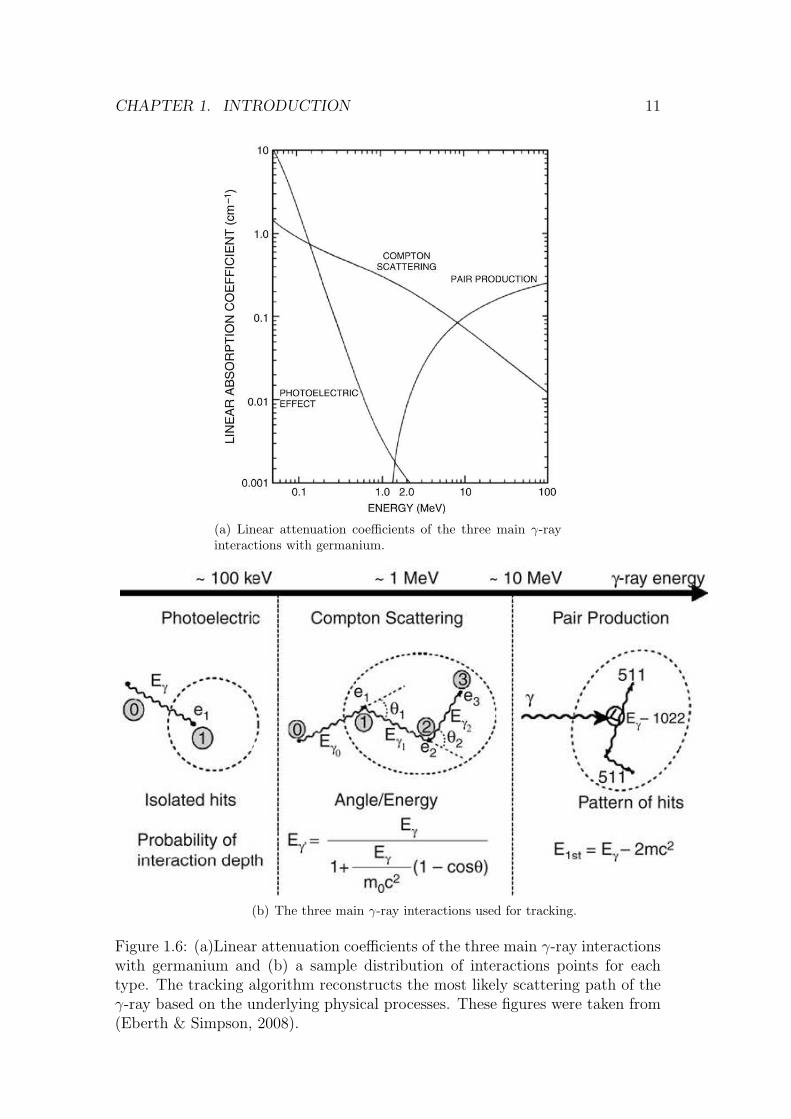
The basic idea of tracking is to reconstruct the most likely scattering path ofthe γ-ray within the detector using the underlying interaction processes namelythe Compton scattering, pair production and the photoelectric effect. As can beseen from figure 1.6(a) the probability of each interaction type to occur is stronglydependent on the γ-ray energy and the distribution of interaction points arecharacteristic for each type (see fig. 1.6(b)). These characteristics are exploited
3The efficiency of an ideal Ge-shell (r1 = 12cm, r2 = 21cm) is ε = 70% and P/T = 78% forMγ = 1 (Schmid et al., 1999).
CHAPTER 1. INTRODUCTION 11
(a) Linear attenuation coefficients of the three main γ-rayinteractions with germanium.
(b) The three main γ-ray interactions used for tracking.
Figure 1.6: (a)Linear attenuation coefficients of the three main γ-ray interactionswith germanium and (b) a sample distribution of interactions points for eachtype. The tracking algorithm reconstructs the most likely scattering path of theγ-ray based on the underlying physical processes. These figures were taken from(Eberth & Simpson, 2008).

CHAPTER 1. INTRODUCTION 12
by tracking, to which there currently two distinctively different approaches. Theback-tracking algorithm starts out by picking the most likely end point of theγ-ray track utilizing the fact that the most probable energy deposit of the finalphotoelectric interaction is in the energy range from ∼ 100 keV to 250 keV .This feature was shown to be independent of the initial energy of the γ-ray(van der Marel & Cederwall, 1999). The upper limit is extended to 600 keV forAGATA since close lying interaction points are packed together. Step by stepfurther points are added to the track and checked for concordance with the eventkinematics. The algorithm stops if the total probability for the scattering pathreaches a certain threshold or a maximum of 5 interaction points are combinedinto a path. The first step of the forward-tracking algorithm (Schmid et al.,
Figure 1.7: The so-called ‘world map’view, used in the forward tracking, of asimulated event with 30 simultaneouslyemitted γ-rays of Eγ = 1MeV . Thecorrectly identified clusters belongingto a single γ-ray are encircled and thosewrongly combined are marked by greenrectangles. This figure is taken from(Gerl & Korten, 2001).
1997) is to calculate the angular coordinates (θ, φ) and the angular separation ofall points (see fig.1.7). These points are then assigned to several clusters, withno cluster containing more than six points and the maximum allowed angularseparation being varied in steps. As the Compton scattering cross section peaksin forward direction and the mean free path of photons decreases with decreasingenergy, the clusterisation procedure is justified. The initial energy of the γ-ray istaken to be the sum of all energy deposits belonging to the clustered interactionpoints. For all permutations of the contained points a figure of merit (FOM),given by the kinematics, is calculated and the ordering having the best FOM ischosen. A comparison of both approaches for AGATA showed forward tracking tobe more efficient (Lopez-Martens et al., 2004). A prerequisite for both algorithmsis the determination of the location, energy and time of each individual interactionpoint.
The precise reconstruction of these parameters is achieved by means of Pulse
Shape Analysis (PSA) and is one major topic of this thesis (see chap. 4). Theaccuracy of the tracking algorithms naturally depends on the precision of PSA.Time differences between individual interaction points are only used to suppress

CHAPTER 1. INTRODUCTION 13
random background and define correlated interactions but cannot be used by thetracking algorithm. Based on simulations of such arrays the position resolutionshould be < 5mm and the energy resolution < 3 keV (Schmid et al., 1999; Lopez-Martens et al., 2004). However, the performance of tracking is more dependent onthe former than on the latter (Schmid et al., 1999). Since neither of the previouslyused detectors are capable of such a high position resolution and planar detectorshaving been ruled out due to an unfavorable ratio of active-to-dead material a newtype of detector, the Highly Segmented Ge detector had to be developed. Severalgroups (e.g. (Vetter et al., 2000b; Vetter et al., 2000a; Kroll & Bazzacco, 2001))contributed to the development and showed that in principle position resolutionsin the range of 2− 4mm can be obtained. Yet, a prerequisite for this is a properunderstanding and simulation of the detectors response, the second major topicof this thesis (see 3). The current consensus is that 36-fold segmented closed-endcoaxial n-type high purity germanium (HPGe) detectors represent the best choicefor realizing a tracking array. Additionally, a tracking array has to be able tosustain high count rates since the most likely experimental conditions will featureeither a high background from the radioactive ion beams or a stable beam withhigh luminosity, i.e. a high event rate, to also populate the weakest channels inthe examined reactions.
Given the expected high costs of such an array and the highly demandingresearch and development to be carried out a European collaboration with thename of Advanced GAmma Tracking Array (AGATA) was established and theinitial memorandum of understanding was signed by 10 countries in 2003. Similardevelopments in the USA lead to the establishment of the GRETA (Gamma Ray
Energy Tracking Array) collaboration. The first topic to be addressed had to bethe number of detectors to be used as this has a significant influence on the datarate and thus the real time requirements of the PSA and tracking algorithms.The stated goal is to cover as much of the 4π solid angle as possible with ac-tive material already ruling out cylindrical detector shapes. The question of thegeodesic tiling of a sphere, i.e. with regular polygons, has already been addressedby Archimedes and the solution contains 12 pentagons and in the simplest case20 hexagons. There are various numbers of hexagons possible and based on theresults of several simulations suggesting between 100-200 detectors needed for atracking array (Eberth & Simpson, 2008) the decision was taken that AGATA willuse 180 detectors with three different hexagonal shapes (see sec. 2.1.1). Thesedetectors will be housed in 60 identical triple clusters (3 crystals per cryostat)and the pentagonal elements will be left free for the beam line and the supportstructure. The inner radius of the sphere will be 23.5 cm and 82% of the solidangle will be covered by the 363 kg of germanium. GRETA will use 120 detectorswith two different shapes housed in 30 clusters of 4 detectors each. The innerdiameter of GRETA will be smaller than AGATA’s leaving less space for ancillarydetectors. Both collaborations will start with sub-arrays to deliver the proof ofprinciple showing that tracking is in fact feasible. AGATA will start with the so-

CHAPTER 1. INTRODUCTION 14
Figure 1.8: Possible geodesic tilings of the sphere. The number of pentagonsremains constant at 12. This figure was taken from (Eberth & Simpson, 2008).
Array No. Crystals Total Granularity ǫFE [P/T ] (%)
EUROBALL III 239 239 9 [56]GAMMASPHERE 110 ∼170 9 [63]
AGATA Demonstrator 15 540 7 [7]AGATA 4π 180 6480 43 [58]GRETA 4π 120 4320 40 [53]
Table 1.1: A summary of the performance of current and future detector arraysfor a γ-ray of 1MeV and a multilpicity of Mγ = 1.
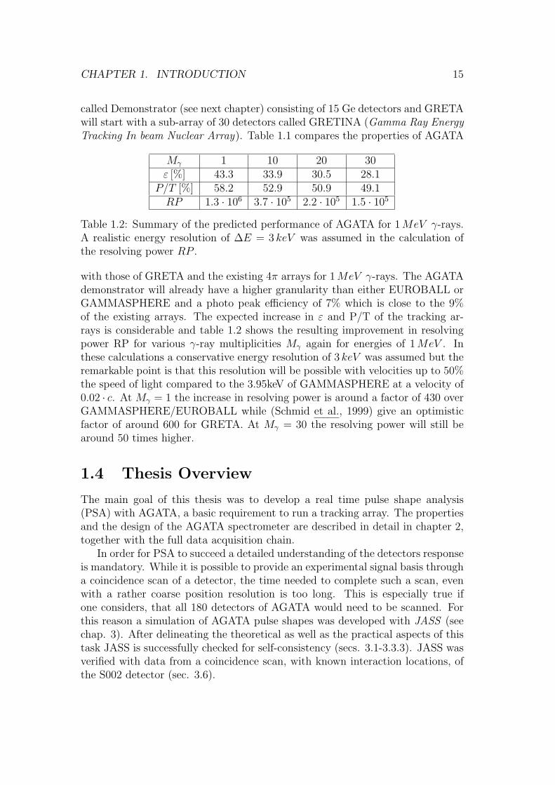
CHAPTER 1. INTRODUCTION 15
called Demonstrator (see next chapter) consisting of 15 Ge detectors and GRETAwill start with a sub-array of 30 detectors called GRETINA (Gamma Ray Energy
Tracking In beam Nuclear Array). Table 1.1 compares the properties of AGATA
Mγ 1 10 20 30ε [%] 43.3 33.9 30.5 28.1
P/T [%] 58.2 52.9 50.9 49.1RP 1.3 · 106 3.7 · 105 2.2 · 105 1.5 · 105
Table 1.2: Summary of the predicted performance of AGATA for 1MeV γ-rays.A realistic energy resolution of ∆E = 3 keV was assumed in the calculation ofthe resolving power RP .
with those of GRETA and the existing 4π arrays for 1MeV γ-rays. The AGATAdemonstrator will already have a higher granularity than either EUROBALL orGAMMASPHERE and a photo peak efficiency of 7% which is close to the 9%of the existing arrays. The expected increase in ε and P/T of the tracking ar-rays is considerable and table 1.2 shows the resulting improvement in resolvingpower RP for various γ-ray multiplicities Mγ again for energies of 1MeV . Inthese calculations a conservative energy resolution of 3 keV was assumed but theremarkable point is that this resolution will be possible with velocities up to 50%the speed of light compared to the 3.95keV of GAMMASPHERE at a velocity of0.02 · c. At Mγ = 1 the increase in resolving power is around a factor of 430 overGAMMASPHERE/EUROBALL while (Schmid et al., 1999) give an optimisticfactor of around 600 for GRETA. At Mγ = 30 the resolving power will still bearound 50 times higher.
1.4 Thesis Overview
The main goal of this thesis was to develop a real time pulse shape analysis(PSA) with AGATA, a basic requirement to run a tracking array. The propertiesand the design of the AGATA spectrometer are described in detail in chapter 2,together with the full data acquisition chain.
In order for PSA to succeed a detailed understanding of the detectors responseis mandatory. While it is possible to provide an experimental signal basis througha coincidence scan of a detector, the time needed to complete such a scan, evenwith a rather coarse position resolution is too long. This is especially true ifone considers, that all 180 detectors of AGATA would need to be scanned. Forthis reason a simulation of AGATA pulse shapes was developed with JASS (seechap. 3). After delineating the theoretical as well as the practical aspects of thistask JASS is successfully checked for self-consistency (secs. 3.1-3.3.3). JASS wasverified with data from a coincidence scan, with known interaction locations, ofthe S002 detector (sec. 3.6).

CHAPTER 1. INTRODUCTION 16
An introduction to the second main topic of this thesis, real-time pulse shapeanalysis is presented in chapter 4. This challenging task is split into the followingtwo sequential parts:
• Determination of the starting time t0 of the recorded pulse shapes.
• Reconstruction of the positions and energy deposits of the individual inter-actions.
The starting time t0 can be identified independently of the position reconstructionand moreover, a predetermined t0 facilitates the remaining PSA task considerably.Feedforward neural networks, which are introduced in section 4.2 are used for theidentification of t0, as they do not only require little computation time but alsooffer a predictable performance, a fact that is very important in a real-time settingas with AGATA. In order to achieve a precise position reconstruction in real-time,evolutionary algorithms offer the most promise. One such algorithm, the so called
”Particle Swarm Optimization “ (PSO, sec. 4.3) provides a framework that is
well suited to the problem at hand. The above presented approach is first appliedto model problems in chapter 5. In chapter 6 data from a GEANT simulation ofa 48Ti(d, p)49Ti reaction at 100MeV under inverse kinematics is used to assessits capabilities under realistic conditions.

Chapter 2
The Advanced Gamma Ray
Tracking Array
The design of AGATA encompasses two main goals. First AGATA had to meetthe requirements for a γ-tracking array (see sec. 1.3) and secondly its layoutshould be highly modular to allow for a stepwise completion of the array. Thefull 4π array will consist of 180 36-fold segmented HPGe detectors with optimizedgeometries (see sec. 2.1). Three of these detectors are combined into identicaltriple cluster detector units and run independently. One such triple cluster has114 output channels, about equal in number to those of existing 4π arrays likeGammasphere. The complete AGATA array will hence have a total of 6840channels, posing a considerably challenge for the data acquisition (DAQ). Inorder to be able to store the experimental data the DAQ has to reduce the datato usable sizes in real-time (see sec. 2.2).
Figure 2.1: Schematic drawing of theAGATA Demonstrator. The five tripleclusters are arranged in such a way thatthey leave a pentagonal hole for thebeam line in the middle. The holdingstructure, shown in red, is easily ex-pandable to allow adding further clus-ters once they are available. This figurewas taken from (Simpson et al., 2008).
The AGATA array is being developed in several key phases:
• The AGATA demonstrator (see fig. 2.1), consisting of 5 triple clusters iscurrently stationed at INFN Legnaro for use with the PRISMA spectrom-eter (Gadea et al., 2005). After the end of the commissioning phase, and
17

CHAPTER 2. THE ADVANCED GAMMA RAY TRACKING ARRAY 18
the accompanying successful proof of principle, the physics campaign willcommence later in 2009, using stable ion beams.
• New triple clusters will be added to the demonstrator in successive steps,once they are fully assembled and tested. It is currently planned that thisevolving array will be moved to GSI/FAIR in Germany 2011/12. ThereAGATA will be used at the focal plane of the fragment recoil separator(FRS) to study exotic nuclei produced following high energy fragmenta-tion. GANIL in France is a likely future host laboratory. The host labora-tories offer a large variety of conditions under which AGATA will be tested,allowing one to properly assess its performance and capabilities.
• Development of the demonstrator into a 1π array, consisting of 15 tripleclusters, followed by a continuous expansion to 4/3π and finally the full 4πAGATA array.
In the following the design of the AGATA components and the data acquisitionsystem will be described in detail.
2.1 The Design of AGATA
The chosen design of AGATA aims on the one hand to fulfill the requirement ofa tracking array (see sec. 1.3) while at the same time to have a setup, which fea-tures a high modularity and symmetry in terms of an arbitrary exchangeabilityof individual components. The full 4π AGATA array will consist of 180 elec-tronically segmented, tapered, encapsulated n-type HPGe detectors. There arethree different asymmetric hexagonal shaped geometries for the detectors whichare housed in one of 60 identical triple cryostats. Each cryostat contains one de-tector of each shape. The resulting germanium shell is 9 cm thick and has a solidangle coverage of up to 82%. The inner radius of the shell is 23.5 cm providingenough space for most ancillary detectors to be mounted inside the shell.
2.1.1 The AGATA crystals
All 36-fold segmented detectors are manufactured out of coaxial HPGe crystals.Each crystal is 90±1mm long and has a diameter of 80+0.7
−0.1mm. In order for thedetectors to be able to form a close packed shell with maximal solid angle coveragethey have to be tapered at the front into a hexagonal shape with a tapering angleof 8. The three different geometries used for the AGATA crystals differ only inthe shape of the hexagonal front face (see fig. 2.3). Each geometry is assigned aletter and a color: A/red, B/green and C/blue. The symmetric prototype usedin the R&D phase of AGATA is labeled S/yellow. The longitudinal segmentationcreates segment rings of 8, 13, 15 , 18 , 18 and 18 mm width (see fig. 2.2(a)) and
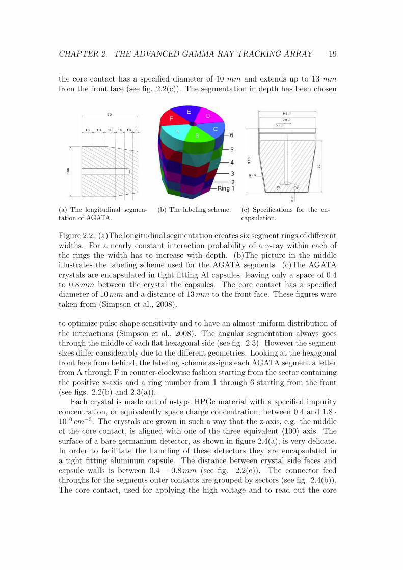
CHAPTER 2. THE ADVANCED GAMMA RAY TRACKING ARRAY 19
the core contact has a specified diameter of 10 mm and extends up to 13 mmfrom the front face (see fig. 2.2(c)). The segmentation in depth has been chosen
(a) The longitudinal segmen-tation of AGATA.
(b) The labeling scheme. (c) Specifications for the en-capsulation.
Figure 2.2: (a)The longitudinal segmentation creates six segment rings of differentwidths. For a nearly constant interaction probability of a γ-ray within each ofthe rings the width has to increase with depth. (b)The picture in the middleillustrates the labeling scheme used for the AGATA segments. (c)The AGATAcrystals are encapsulated in tight fitting Al capsules, leaving only a space of 0.4to 0.8mm between the crystal the capsules. The core contact has a specifieddiameter of 10mm and a distance of 13mm to the front face. These figures waretaken from (Simpson et al., 2008).
to optimize pulse-shape sensitivity and to have an almost uniform distribution ofthe interactions (Simpson et al., 2008). The angular segmentation always goesthrough the middle of each flat hexagonal side (see fig. 2.3). However the segmentsizes differ considerably due to the different geometries. Looking at the hexagonalfront face from behind, the labeling scheme assigns each AGATA segment a letterfrom A through F in counter-clockwise fashion starting from the sector containingthe positive x-axis and a ring number from 1 through 6 starting from the front(see figs. 2.2(b) and 2.3(a)).
Each crystal is made out of n-type HPGe material with a specified impurityconcentration, or equivalently space charge concentration, between 0.4 and 1.8 ·1010 cm−3. The crystals are grown in such a way that the z-axis, e.g. the middleof the core contact, is aligned with one of the three equivalent 〈100〉 axis. Thesurface of a bare germanium detector, as shown in figure 2.4(a), is very delicate.In order to facilitate the handling of these detectors they are encapsulated ina tight fitting aluminum capsule. The distance between crystal side faces andcapsule walls is between 0.4 − 0.8mm (see fig. 2.2(c)). The connector feedthroughs for the segments outer contacts are grouped by sectors (see fig. 2.4(b)).The core contact, used for applying the high voltage and to read out the core

CHAPTER 2. THE ADVANCED GAMMA RAY TRACKING ARRAY 20
−40 −20 0 20 40−40
−30
−20
−10
0
10
20
30
40
X [mm]
Y [m
m]
C B
A
FE
D
(a) Angular segmentation of the symmetricprototype.
−40 −20 0 20 40−40
−30
−20
−10
0
10
20
30
40
X [mm]
Y [m
m]
(b) Angular segmentation of the red/A typecrystal
−40 −20 0 20 40−40
−30
−20
−10
0
10
20
30
40
X [mm]
Y [m
m]
(c) Angular segmentation of the blue/C typecrystal
−40 −20 0 20 40−40
−30
−20
−10
0
10
20
30
40
X [mm]
Y [m
m]
(d) Angular segmentation of the green/B typecrystal
Figure 2.3: The angular segmentation schemes of all existing AGATA crystals.All segmentation lines go through the middle of each hexagons flat side faces.In order for the array to cover the largest possible solid angle three differentasymmetric hexagonal front faces were necessary with the red type being themost and the blue type the least asymmetric.

CHAPTER 2. THE ADVANCED GAMMA RAY TRACKING ARRAY 21
(a) unsegmented AGATA crystal (b) encapsulated AGATA crystal
Figure 2.4: Picture (a) shows a still unsegmented bare AGATA crystal while inpicture (b) an already encapsulated crystal, viewed from behind, is shown. Thefeed through for the core contact is situated in the middle and slightly elevatedwith respect to the six feed throughs for each segment column on the outside ofthe capsules back side. These figures were taken from (Simpson et al., 2008).
signal, sits in the middle of the capsules back side and is isolated by ceramics.Besides the geometrical characteristics an AGATA crystal also needs to fulfillstringent requirements in term of energy resolution (see tab. 2.1) before it isaccepted by the collaboration.
Energy Core Contact Segment Mean of Segments
1.3MeV ≤ 2.35 keV ≤ 2.30 keV ≤ 2.10 keV122 keV ≤ 1.35 keV - -60 keV - ≤ 1.30 keV ≤ 1.20 keV
Table 2.1: The specifications for the energy resolutions (FWHM) of the AGATAcrystals. For the segments the specifications define an upper limit for each seg-ment individually and also for the mean resolution of all segments.
2.1.2 The AGATA cryostats
The cryostats do not only house the three AGATA crystals but also the coldand warm part of the preamplifiers (see sec. F.1), which have to be mountedclose to the detectors in order to minimize noise contributions. The cold partsof the preamplifiers are operated at a temperature around 130 K where their
CHAPTER 2. THE ADVANCED GAMMA RAY TRACKING ARRAY 22
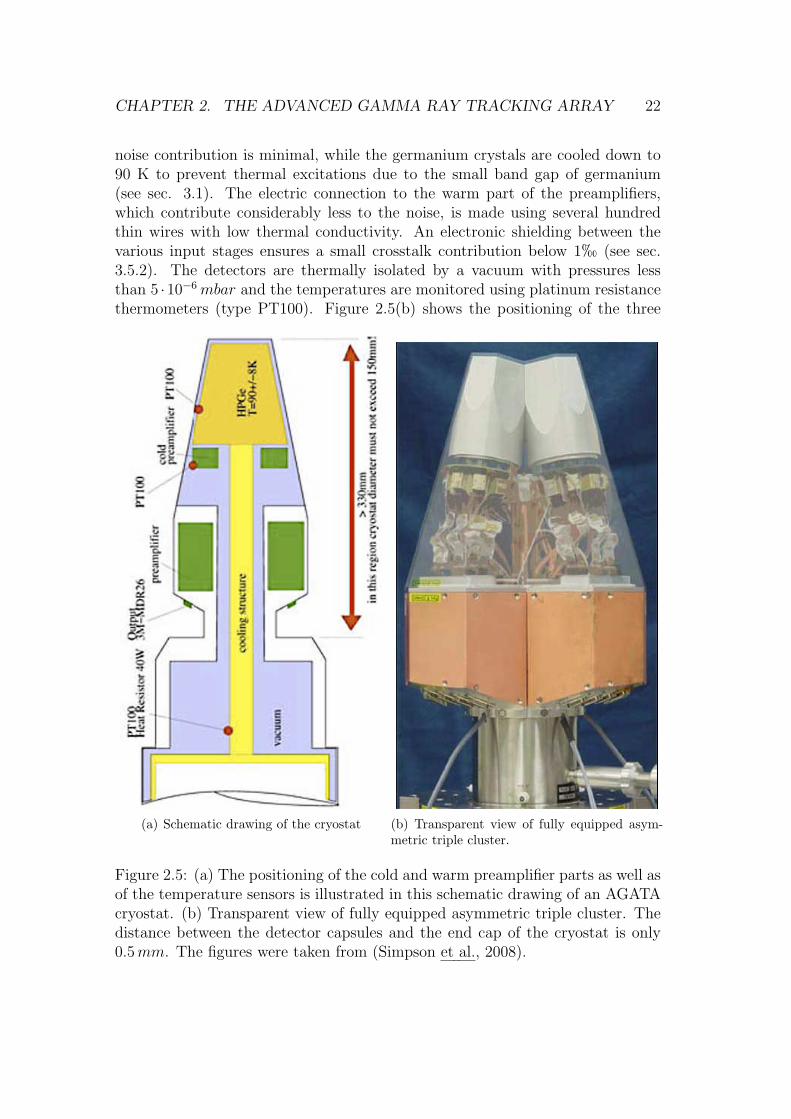
noise contribution is minimal, while the germanium crystals are cooled down to90 K to prevent thermal excitations due to the small band gap of germanium(see sec. 3.1). The electric connection to the warm part of the preamplifiers,which contribute considerably less to the noise, is made using several hundredthin wires with low thermal conductivity. An electronic shielding between thevarious input stages ensures a small crosstalk contribution below 1h (see sec.3.5.2). The detectors are thermally isolated by a vacuum with pressures lessthan 5 ·10−6mbar and the temperatures are monitored using platinum resistancethermometers (type PT100). Figure 2.5(b) shows the positioning of the three
(a) Schematic drawing of the cryostat (b) Transparent view of fully equipped asym-metric triple cluster.
Figure 2.5: (a) The positioning of the cold and warm preamplifier parts as well asof the temperature sensors is illustrated in this schematic drawing of an AGATAcryostat. (b) Transparent view of fully equipped asymmetric triple cluster. Thedistance between the detector capsules and the end cap of the cryostat is only0.5mm. The figures were taken from (Simpson et al., 2008).

CHAPTER 2. THE ADVANCED GAMMA RAY TRACKING ARRAY 23
detectors relative to the end cap, which has been rendered semi-transparent.The warm part of the preamplifiers is hidden under the copper plates. Current4π spectrometers operated today have a total of 100 to 200 channels to be readout, comparable to the 114 channels of a single triple cryostat for AGATA.
A triple cluster unit weighs 38 kg without the germanium crystals and has alength of 92 cm demanding rather rigid holding structures since the clusters haveto be positioned with high precision in the array. First of all because thermalconductivity between the end caps, there is a narrow 0.5mm wide spacing betweenadjacent end caps, has to be prevented and even more importantly to ensure anaccurate tracking (see sec. 1.3). There are very low tolerances required for themanufacturing of the end caps as well, which have to stay within specificationseven when bending under vacuum.
2.2 The AGATA Data Acquisition
The AGATA data acquisition (DAQ) system consists of two basic building blocks,one is hardware based comprising the detectors, preamplifiers, digitizers and thefront-end electronics, and the second is software based running on PC serverfarms. In addition to processing and transporting the data, the DAQ is alsoresponsible for controlling and monitoring the complete DAQ system, includingall the algorithms running on the servers. This second task as well as the datahandling on the server farms is carried out by the Nouvelle Acquisition temp Reel
Avec Linux, (Grave et al., 2005), or NARVAL system. In the following the dataflow, as depicted in figure 2.6, will be described and each component explainedin separate sections.
The signals from the detectors are read out by charge-sensitive preamplifiersand then continuously digitized by sampling 14 bit Analog-to-Digital converters(ADC) at a rate of 100 MHz. The data rate out of each digitizer channel is200 MBytes/sec, independent of the detectors event counting rate as 100% ofthe incoming signals are digitized. The front-end electronics assigns an eventtime and number, determines the energy depositions using the Moving Window
Deconvolution (Georgiev et al., 1994) and extracts the useful parts, also called theleading edges, of the traces. These parts are about 6µs long and contain parts ofthe baseline, the complete rise time of the signal and parts of the exponentiallydecaying charge signal, recorded once all charge carriers created by the γ-rayinteraction are collected. The latter takes up the most part of the extracted tracesand is used by the MWD algorithm. This data package is reduced to 600ns andthen sent to the PSA algorithm with data rates of up to 370 MBytes/sec. Fromthis point on, marked by using red borders in figure 2.6, all the data is beinghandled on the servers. The interaction positions are then reconstructed by thePSA and the event builder merges all corresponding locations, and optionallydata from an ancillary detector to form a single event. The tracking algorithm

CHAPTER 2. THE ADVANCED GAMMA RAY TRACKING ARRAY 24
AGATA Triple Cluster with preamplifiers
DigitizerDigitizer Digitizer
Front End
Electronics
Front End
Electronics
Front End
Electronics
PSAPSA PSA
Event
Builder
MergingAncillary
Detector
Tracking
Storage
Figure 2.6: The AGATA Data Flow for one triple cluster. The preamplifiers forthe signals are housed in the cryostat, together with the encapsulated crystals.The pulse shapes are then digitized and moved to the front end electronics usingoptical fibers. All the data is then sent to the PSA farms. The reconstructedpositions in the three crystals are combined in the event builder. At this stagethe data can optionally be merged with data from an ancillary detector. Finallytracking reconstructs the scattering path(s) of the γ-ray(s) and the data is storedonto mass storage devices.

CHAPTER 2. THE ADVANCED GAMMA RAY TRACKING ARRAY 25
then uses this information to reconstruct the most likely scattering path of theγ-ray(s). Finally the data will be stored onto a local file server before beingeventually sent to a Grid Tier 1 computing center. For a more detailed descriptionof the individual electronic components of the DAQ chain the interested readeris referred to appendix F.

Chapter 3
JASS - Simulating Agata Pulse
Shapes
The basic approach to real-time pulse shape analysis (PSA) for AGATA is tosearch a basis set of available pulse shapes, with known interaction locations, foragreement with the experimnetal signal (see chap. 4). Hence it is imperativeto have a precise knowledge of the detectors response as this directly influencesthe precision of the PSA. While a conventional coincidence scan can, in principleprovide such a basis (Boston et al., 2007), it still takes about two months tocomplete for 2000 points out of the roughly 300000 needed for a basis on a 3-D gridwith 1 mm steps. This is a far too long time frame considering that AGATA willconsist of 180 detectors, with each one needing to be scanned. Additionally, as willbe shown in section 3.6.1, the uncertainties of the scanning setup are too large toallow the production of a finely sized basis set. Therefore, an accurate simulationof the pulse shapes had to be developed. In the course of this work it becameclear that the previous approach, using the Multi Geometry Simulation (Medinaet al., 2004) suffered from inconsistencies especially at the segment boundaries.This prompted the development of JASS, the Java Agata Signal Simulation, inthe frame work of this thesis.
In section 3.1 an introduction into the field of simulating pulse shapes isgiven. The peculiarities regarding germanium and the novel methods employedby JASS are discussed in sections 3.2 and 3.3. The electronic response functionsand the detector specific influence on the signal shape due to crosstalk, neededbefore any comparison with experimental signals can take place, are presentedin section 3.5. Finally, in section 3.6 the JASS calculations are verified usingexperimental data from a simple pencil beam as well as data from a coincidencescan with known interaction locations. The chapter closes with an outlook anddiscussion in section 3.7.
26

CHAPTER 3. JASS - SIMULATING AGATA PULSE SHAPES 27
3.1 Simulation of HPGe Pulse Shapes
Given an interaction at position P (x, y, z) within the germanium crystal a certainnumber of electron-hole pairs are created. However, these pairs are not createddirectly by the γ-ray but by the asociated Compton-/photo electron, or from e+e−
pair production, which has a mean free path length of about 1mm at 1MeV .While the band gap of germanium is 0.74 eV at 90K it takes on average 2.96 eVto create an electron hole pair due to the competing process of exciting latticevibrations. Hence for a 1 MeV interaction around 3.4 · 105 electron-hole pairsare created. In contrast to the charge clouds of electrons and holes in reality, asimulation assumes point-like charge carriers. This is justified, as in large volumedetectors the expansion of the charge clouds, due to space charge, is negligible(Medina, 2006). For n-type germanium, like the AGATA crystals the holes (h)are drifting to the outer electrodes while the electrons (e−) are collected at thecentral core contact (Knoll, 1999). The only observables of this event are thecharge signals Qi(t) induced by the moving charge carriers qe/h on the electrodesi. This raises the two following questions:
• How do the charge carriers qe/h move through the crystal?
• What signals Qi(−−→re/h(t)) are induced at the electrodes i?
Each part of the problem can be treated separately by using a quasi steady-state approximation. First, the assumption is made that the momentary electricfields are in electrostatic equilibrium, which is justified as the speed of the chargecarriers ∼ 107cm/s is small compared to the speed of light in germanium cGe =750·107cm/s. Additionally, it is assumed that the perturbation to the electric field~E inside the crystal, caused by the presence of the charges qe/h has a negligibleinfluence on the charge carriers movement.
The trajectories of the charge carriers therefore are solely influenced by ~Eand the crystal structure (see sec. 3.2), reducing the problem to electrostatics.The calculation of the electric field is a problem of mostly practical nature andis delineated in section 3.2.2. The effect of the crystal orientation on the chargecarriers trajectories, however does take some theoretical understanding. It isowing to the band structure of germanium, resulting in an anisotropy of the drifttimes. Moreover this anisotropy is different for electrons and holes. The modelsdescribing this behavior can be found in the literature and are summarized insections 3.2.3 and 3.2.4. As pointed out in detail in section 3.2.1, a precisedescription of the detectors geometry is also vital for a successful simulation.
Since the electric fields are considered to be in equilibrium the charge signalsat time t are dependent on the momentary position of the charge carriers ~r(t)only. Under this assumption the calculation of the pulse shapes (see sec. 3.3) canbe greatly simplified as the Shockley-Ramo theorem, described in section 3.3.1is applicable. But the multitude of electrodes in a highly-segmented detector

CHAPTER 3. JASS - SIMULATING AGATA PULSE SHAPES 28
brings about a high variability in the pulse shapes. Thus the limited precision ofa numerical solver must be enhanced by a precise interpolation method (see sec.3.3.3).
3.2 Calculating the Trajectories
In order to calculate the trajectories of the charge carriers the velocity vectorof their motion through the crystal must be determined. The general relationbetween the drift velocity −→vd and the electric field ~E is quite simple and givenby:
−→vd = ±µ(| ~E|) · ~E (3.1)
with the mobility µ, which is influenced by the crystal structure. The minus signis used for electrons to make them flow in the opposite direction of the appliedelectric field.
It is therefore necessary to understand how the crystal structure of germaniumis affecting the mobilities of the charge carriers. The scalar behavior of themobility in equation 3.1 only holds at low fields though. Once the fields becometoo strong the mobility is turning into a tensor µ(| ~E|). Only then it is influencedby the band structure of germanium. This influence is best described using thereciprocal lattice vectors ~k. In semiconductors the charge carriers occupy theoptima or band edge of the respective band structure. In the simple case ofa non-degenerate band structure and the band edge being at the center of theBrillouin zone a strictly parabolic relationship between the energy ǫ and the wavevector ~k results (see (Conwell, 1967) p.49)
ǫ(~k) =~
2k2
2m, (3.2)
with m the effective mass of the charge carrier, typically differing from the freeelectron mass m0. In this case one observes an isotropic distribution of drifttimes as the drift velocity of a single charge carrier is related to ǫ(~k) through thefollowing equation:
~v(~k) =1
~
−→∇kǫ(~k). (3.3)
It should be noted that the isotropy of the drift velocities is independent of thedistribution of ~k-states for all charge carriers. Germanium, by contrast to thissimple picture, has a so-called many valley band structure with the charge carrierseither occupying many equivalent valleys in the case of electrons or a twofolddegenerate band in the case of holes. One resulting feature is that the currentneed not be parallel to the applied electric field. First experimental evidence ofthis was reported by (Sasaki & Shibuya, 1956). As presented later, the observedanisotropies of the drift velocities can all be understood in terms of deviations of
CHAPTER 3. JASS - SIMULATING AGATA PULSE SHAPES 29
the ǫ − k relationship from eqn. 3.2. Since these deviations are different for theconduction and the valence band one needs distinct models for both cases.
As pointed out earlier, the internal crystal fields are neglected and all anisotropiesare covered by the mobility model. So all it takes to calculate the electric fieldis to solve the Poisson equation. In order to be able to represent the boundaryconditions of the Poisson equation accurately an equally accurate description ofthe crystals geometry is needed and for reasons detailed in section 3.2.1 it is ad-vantageous not to drop this precise information after the Poisson equation hasbeen solved.
3.2.1 Description of the Geometry
An easy way to describe an extended object for a computer program is to use aregular grid of points and each one being labeled as either outside or inside theobject. For a given interaction location in the crystal point-like charge carriersare drifted according to the electric field and equation 3.1. Yet, as the electricfield and the detector boundaries are only available in the precision of the finitegrid it is likely that the charge carriers would drift into unphysical regions andnot stop at the correct boundary. Also, chances are that the hit segment for aninteraction location will be wrongly identified if the end point of the trajectoryis in close vicinity of the unresolved segment boundaries. A fine enough grid toprevent this would most certainly need excessive computing resources.
JASS takes another approach to define the geometry and explicitly uses theequations used for manufacturing the crystals and an adequate model for thecore contact. The shape of the latter is modeled as a cylinder with a sphericalend and its tip being 13 cm from the front face of the crystal. It’s characteristicradius is Rcore = 5.5mm. A 2D cut of the crystal definition is shown in figure3.4.
The surface of each AGATA crystal, however, has a rather irregular shape.The front part of a crystal is hexagonal while the back part is coaxial withan intermediate stage in between. Despite this irregularity a description withnumerical precision is rather easily achieved. The coaxial contribution is modeledas a cylinder with radius Rc = 40mm and depth dc = 90mm. The hexagonal partis defined by the intersection of six planes, which are tilted away from the z-axis.Each plane is given by two pairs of points defining the straights of intersectionwith its neighboring planes. The surface of the crystal defines a set of points eitheron one plane or the cylinder, whichever is closest to the z-axis. The transitionarea from the hexagonal to the coaxial structure is defined by the conic sections ofthe planes with the cylinder. As an example the resulting shape for the symmetricAGATA prototype is shown in figure 3.1.
To enable the simulation to stop the charge carrier at the correct boundary acriterion must be formulated to determine, with numerical precision, whether apoint P (x, y, z) is inside or outside the crystal. So it has to be shown that P is

CHAPTER 3. JASS - SIMULATING AGATA PULSE SHAPES 30
Figure 3.1: This figure shows thesurface of the symmetric AGATAprototype crystal as it is reproducedby JASS. One can clearly see thatthe front part is hexagonal while theback areas are coaxial. The line ofintersection for any of the six planeswith the cylinder, defining also thetransition from the hexagonal to thecoaxial geometry is a conic sectionwith hyperbolic shape.
inside the cylinder and at the same time on the same side of each plane as theorigin point P (0, 0, 0). In the case of the cylinder this is trivial as only the radialposition of P and 0mm < z < 90mm has to be checked . Concerning the planesit is best to write the plane equations in Hesse’s Normal Form (see app. C) asthen the distance δ of the point P from the plane is calculated by:
δ = x cosα+ y cos β + z cos γ − p. (3.4)
The angles α, β and γ define the direction of the plane’s normal vector and p isit’s distance to the origin. For a negative δ the point is on the same side of theplane as the origin (see e.g. (Bronstein, 2000), pp. 221). A test charge thereforereaches the boundaries of the crystals active volume if it either reaches the corecontact or the outside, as described above. Hence the point P (x, y, z) is insidethe active volume of the crystal as long as the following conditions are met:
δ < 0 ∀ planes√
x2 + y2 < Rc
0 ≤ z ≤ dc√
x2 + y2 ≥ Rcore for z > 18.5√
x2 + y2 + (z − 18.5)2 ≥ Rcore for 13.0 ≤ z ≤ 18.5 (3.5)
Using this model the test charges are stopped within less than 10 µm of the true

CHAPTER 3. JASS - SIMULATING AGATA PULSE SHAPES 31
boundary 1 enabling the simulation to correctly identify the hit segment withinthe accuracy of the trajectory.
3.2.2 Calculation of the Electric Field
As pointed out in the introduction the most important component necessary tocalculate the trajectories of the electrons and holes is the electric Field ~E(~r).The electric field can be obtained by solving the Poisson equation for the poten-tial Φ(~r) under adherence to the boundary conditions, precisely defined at thelocation of the electrical contacts:
∇2Φ(~r) = − ρ(~r)
ε0 εr
(3.6)
with parameters space charge distribution ρ(~r) and the dielectric constant ofgermanium εr = 16. The electric field is simply given by the gradient of Φ(~r).
Due to the complex geometry, however, there is no analytical solution to thePoisson equation for the AGATA crystals, leaving numerical methods as the onlyoption. Hence the problem is discretized on a regular rectangular grid with a gridsize still to be determined. This choice of grid type is related to the choice for aniterative finite difference algorithm (see app. D) to solve the equation. This classof algorithms uses the finite difference quotient (see app. D.1) to approximate theleft hand side of equation 3.6 and solves the resulting equation for the potentialΦ(~r). The time for the algorithm to converge is not a constraint on the algorithmas the electric field has to be calculated only once per crystal. While there arefaster converging methods available, JASS employs the Red-Black Gauß-Seidelalgorithm (see (Trottenberg et al., 2000), p. 31 and app. D.2.1) for its easeof use and memory efficiency. Before the algorithm starts the grid is split intoodd and even indexes2 since only the values from the even indexes are needed toupdate the odd indexes and vice versa. This is evident by using central differenceapproximation to the to the left hand side of equation 3.6 and solving for Φ(x, y, z)(see app. D for details):
Φi+1(x, y, z) =ε0 εr(ΣΦi
x + ΣΦiy + ΣΦi
z) + ρx,y,z ∆r2
6 ε0 εr
(3.7)
with ΣΦix = Φi(x+ 1, y, z) + Φi(x− 1, y, z) and accordingly for y,z
and the grid size ∆r.
At every iteration i the odd indexes are being updated first so that their valuesfrom iteration i+1 can be used to update the values of the even indexes. Withoutthis ordering of grid points two copies of the grid would have to be kept in
1The precision naturally depends on the time step ∆t used in the discretization of thetrajectory calculation. JASS uses time steps of 0.1ns ( see sec. 3.4).
2These are called the red and black points in reference to the two colors on a roulette wheel.

CHAPTER 3. JASS - SIMULATING AGATA PULSE SHAPES 32
memory, one for the current values from iteration i and one to store the newvalues of iteration i + 1. The solver has converged once the changes from oneiteration to the next are below a given threshold for every grid point.
At this point the size of grid steps necessary to solve the Poisson equationwith a certain accuracy has to be determined. In order to achieve this task a testcase with a known analytical solution is required. The core weighting potential(see sec. 3.3.1 for details) of a true coaxial detector is such a test case which alsooffers a geometry that is at least in parts similar to the AGATA detectors. Thepotential is given by
ψ0(~r) = 1 − ln (r
rmin
)/ ln (rmax
rmin
) (3.8)
While it is clearly advantageous to use a cylindrical grid for a true coaxial de-tector, as the potential has only a radial dependency the situation is differentfor the AGATA crystals. Their shape is dominated by the hexagonal structuredefined by the six planes (see fig. 3.1) making a rectangular grid better suited tothe problem. The core contact is placed in the center of the grid for both cases.A grid spacing of 0.5mm suffices to have a relative error smaller than 1% in thetest case, confirming previous reports for the MINIBALL spectrometer (Bruyneelet al., 2006a).
Due to the absence of space charge in the test case, it is easier to calculatewithin a certain margin of error. Yet, in reality the electric potential is stronglyinfluenced by the impurity concentrations in the germanium crystal making anappropriate model of their distribution a necessity. Figure 3.2 shows the averagespace charge densities as a function of depth within the detector, as providedby the manufacturer. According to current knowledge only the values at theboundaries at z = 0mm and 90mm are measured and the intermediate values areinterpolated linearly, explaining the observed perfect linearity. However, positiveand negative slopes for the different crystals are observed. This is associatedwith the fact that the higher the space charge density the higher the electricfield necessary for a full depletion of the detector. In the case of higher averageimpurity concentrations only a decrease with depth can ensure full depletion atthe nominal core voltage of 5 kV since the highest fields can only be found in thefront part of the detector, especially at the tip of the core contact. Assumingreasonably that the impurity concentration at r = 0 also varies linearly withdepth, coupled with the assumption of cylindrical symmetry as in (Bruyneelet al., 2006b) the distribution is fully characterized by four numbers. For theS002 symmetric prototype detector these are the following (in 1010 · cm−3):
ρ(r = 0, z = 0) = 2.0 ρ(z = 0) = 1.8
ρ(r = 0, z = 90) = 1.0 ρ(z = 90) = 0.51 (3.9)
There are two noteworthy points about the resulting distribution, displayed infigure 3.3 at x = 0. First of all the highest local space charge densities are all

CHAPTER 3. JASS - SIMULATING AGATA PULSE SHAPES 33
0 10 20 30 40 50 60 70 80 90 1000.4
0.6
0.8
1
1.2
1.4
1.6
1.8
2
Depth [mm]
Sp
ace
ch
arg
e d
en
sity
[1
01
0/c
m3]
Space charge densities as provided by manufacturer
S001−SN73838S002−SN73821S003−SN73839A001−SN73952A002−SN73949A002−SN74030A003−SN74009A004−SN74041B001−SN73888B001−SN74034B002−SN73979B003−SN74026C001−SN73899C002−SN73951C003−SN74013C004−SN74036
Figure 3.2: The impurity concentrations for several AGATA crystals, as providedby the manufacturer are plotted as a function of depth (z-direction) within thedetector. The concentrations either increase or decrease linearly with depth.

CHAPTER 3. JASS - SIMULATING AGATA PULSE SHAPES 34
Figure 3.3: The distribution of space charge density for the S002 prototype de-tector at x = 0. Even though the distribution has only a linear dependency onthe depth and the radius, the lines of equal impurity concentration show a clearcurvature. This can be traced back to the fact that also the slope of the radialdistribution changes linearly with depth.

CHAPTER 3. JASS - SIMULATING AGATA PULSE SHAPES 35
located in the center of the crystal, being either in front or just next to the corecontact tantamount to a negative slope for the radial dependency. Secondly thelines of equal density are not straight but show a curvature due to the 2D linearchange.
The only remaining issue is the question of correct boundary conditions. Thesegmentation lines have widths of the order of ∼ 100µm and are therefore ne-glected in the further discussion. Thus there are just two different types of bound-aries of the detector namely the surfaces of the segment and core electrodes aswell as the passivated layer at the back. According to (Mihailescu, 2000) thelatter can ideally be considered as an electrostatic mirror, so homogeneous von-Neumann boundary conditions are applicable:
∇Φ(~r) · −−→n(~r) = 0 ∀~r ∈ ∂Ωback (3.10)
with the normal vector−−→n(~r) and the surface area of the passivated layer ∂Ωback.
Equation 3.10 ensures that the equipotential lines end up perpendicular to thepassivated backside. Dirichlet boundary conditions are used for the electrodes:
Φ(~r) = 5000V ∀~r ∈ ∂Ωcore
Φ(~r) = 0V ∀~r ∈ ∂Ωsegment (3.11)
with the surface area ∂Ωcore of the core and ∂Ωsegment of the segment electrodes,respectively. The electric potential as calculated by JASS for the S002 detectoris pictured in figure 3.4 for a cut at y = 0. There are two features that strikethe eyes. First, high gradient changes of the potential in front of the core con-tact can be observed. These are simply due to the short distance to the outerelectrodes with just 13mm. There are no areas with a comparable high gradientin the test case and thus in this region a limited precision of the numerical solu-tion can be expected. Additionally, the electric field lines in this region have astrong curvature leading to equally curved trajectories of the charge carriers andconsequently to effective segment sizes differing considerably from their physi-cal dimensions (see fig. 3.5). Another observation is the slight warping of theequipotential lines which can be attributed to the impurity distribution and thegeometry of the detector. The presence of a space charge pushes the equipotentiallines closer to the outer electrodes in a manner that is proportional to the localdensity. This explains the warping when seen in conjunction with the increasingdistance between the core contact and the outside of the crystal in the hexagonalpart of the detector. The distance between a given equipotential line and thecentral electrode decreases with depth, as does the impurity concentration whentaken relative to the aforementioned distance.
3.2.3 Mobility of Electrons
The second important ingredient to calculate the signal shape is the mobility ofthe charge carriers (see 3.1). The fact that the electron’s drift velocities within

CHAPTER 3. JASS - SIMULATING AGATA PULSE SHAPES 36
−40 −20 0 20 400
10
20
30
40
50
60
70
80
X [mm]
Z [
mm
]
Po
ten
tial [
V]
0
500
1000
1500
2000
2500
3000
3500
4000
4500
5000
Figure 3.4: Plot of the electric potential inside the S002 AGATA crystal at y = 0.The boundaries of the electrodes are marked in white and the black contour linesindicate steps of 250 V. The strong gradient of the potential in front of thecore contacts tip is easily noticed. This is a likely source of errors which arepossibly larger than those observed in the test case. The apparent warping ofthe equipotential lines is due to an interplay of the detectors geometry and themodel of the impurity distribution.

CHAPTER 3. JASS - SIMULATING AGATA PULSE SHAPES 37
Figure 3.5: The effective segmentation of the yellow AGATA crystal. Due to thecurved electric field in the front the charge carriers do not drift horizontally tothe nearest electrode but to electrodes further to the front. The effective segmentsizes for each row are indicated by different colors with blue showing all locationsfor which the holes are collected in the first row, cyan for those collected by thesecond row segments and so forth.
germanium feature an anisotropy has long been established. (Nathan, 1963), forexample, found that at 77K and low fields, ∼ 100V/cm, the drift velocities ofelectrons in 〈100〉 direction can be as much as 60% larger than in the 〈111〉 direc-tion. At higher fields of around 10000V/cm though this anisotropy is reduced to15%. These results can be understood in terms of an anisotropy of the effectivemasses and looking at the ǫ-k relation (eqn. 3.12). In germanium the minima ofthe conduction band are situated on the intersections of the Brillouin zone withthe four equivalent 〈111〉 directions. Each of the corresponding eight valleys hasa half ellipsoidal shape. A fact that becomes clear when looking at the ǫ − krelation, written in the principal axis system of one such ellipsoid. It is thengiven by (Conwell, 1967):
ǫ(~k) =~
2k2x
2mx
+~
2k2y
2my
+~
2k2z
2mz
(3.12)
with kx,y,z measured from the valley minimum. Considering the y-axis to bethe axis of revolution, ky ≥ 0 results and the effective masses can be written asmy = ml and mx = mz = mt. Reported values (Mihailescu et al., 2000) areml = 1.64m0 and mt = 0.0819m0. This anisotropy of the effective masses leadsto the ellipsoidal shape of the valleys and the anisotropy in the mobility. Figure3.6 shows the ellipsoidal equal energy surface for one valley as given from theabove description.

CHAPTER 3. JASS - SIMULATING AGATA PULSE SHAPES 38
Figure 3.6: The equal energy surfacefor hot electrons revealing the ellip-soidal shape of the valleys. The y-axishas been aligned with the 〈111〉 direc-tion and the boundary of the Brillouinzone is at ky = 0. Comparing equa-tions 3.2 and 3.12 it can be concludedthat the ellipsoidal shape is solely dueto the difference in effective masses.
To facilitate the analytical model the assumption is made that solely the〈111〉 valleys are populated (Reik & Risken, 1962) and a primitive cell is chosenin which the half ellipsoids sitting on the same axis, but at opposite sides of theBrillouin zone, are joint together (Ashcroft & Mermin, 1976). Transforming the
wave vector ~k linearly by ~k∗ = α1/2i~k, with the electron effective mass tensor αi
the ellipsoids, in each of the four remaining valleys become spheres. Using therotation matrix Ri to align the principal axis of the i− th valley with the y-axisof the lab system the tensor is given by
αi = RTi ·
m−1t 0 00 m−1
l 00 0 m−1
t
·Ri (3.13)
To preserve the vector relations the electric field and the drift velocities need to
undergo similar transformations. The former translates just as ~k,−→Ei
∗ = α1/2i~E,
the drift velocity however transforms differently with −→vi∗ = α
−1/2i
−→vi (see eqn.
3.3). Equation 3.1 can then be used in−→ki
∗-space as the valleys take on a sphericalshape and the drift velocities become isotropic (Conwell, 1967; Reggiani et al.,1985)
−→vi∗ = −µ∗(E∗
i )−→Ei
∗. (3.14)
The mobility µ∗ depends only on the amplitude of the effective field strength E∗.From the above equations the total drift velocity −→vd in ~k-space can be calculatedas the weighted average of each valleys drift velocity −→vi
−→vd( ~E) = −4∑
i=1
ni · µ∗(E∗i ) · αi
−→Ei (3.15)
with ni the relative valley population(∑4
i=1 ni = 1).
Figure 3.7 shows the distribution of the electron drift times in the coaxialpart of a symmetric AGATA detector for two different crystal orientations. All

CHAPTER 3. JASS - SIMULATING AGATA PULSE SHAPES 39
100 ns
200 ns
300 ns
400 ns
30
210
60
240
90
270
120
300
150
330
180 0
t 100 , α=35°
t 100 , α=80°
t 9030
, α=35°
t 9030
, α=35°
Figure 3.7: The t100 (solid) and t9030 (dashed) drift times of electrons in the coaxialpart of a symmetric AGATA detector for two different orientations of the crystalaxis. The angle α is the angle between the x-axis in the lab system and thefirst 〈100〉 axis. A simple rotation by ∆α of one distribution makes it coincidewith the other. The drift times themselves seem to oscillate around an isotropicdistribution.
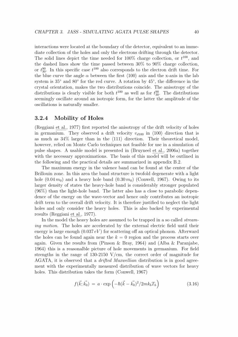
CHAPTER 3. JASS - SIMULATING AGATA PULSE SHAPES 40
interactions were located at the boundary of the detector, equivalent to an imme-diate collection of the holes and only the electrons drifting through the detector.The solid lines depict the time needed for 100% charge collection, or t100, andthe dashed lines show the time passed between 30% to 90% charge collection,or t9030. In this specific case t100 also corresponds to the electron drift time. Forthe blue curve the angle α between the first 〈100〉 axis and the x-axis in the labsystem is 35 and 80 for the red curve. A rotation by 45, the difference in thecrystal orientation, makes the two distributions coincide. The anisotropy of thedistributions is clearly visible for both t100 as well as for t9030. The distributionsseemingly oscillate around an isotropic form, for the latter the amplitude of theoscillations is naturally smaller.
3.2.4 Mobility of Holes
(Reggiani et al., 1977) first reported the anisotropy of the drift velocity of holesin germanium. They observed a drift velocity vd100 in 〈100〉 direction that isas much as 34% larger than in the 〈111〉 direction. Their theoretical model,however, relied on Monte Carlo techniques not feasible for use in a simulation ofpulse shapes. A usable model is presented in (Bruyneel et al., 2006a) togetherwith the necessary approximations. The basis of this model will be outlined inthe following and the practical details are summarized in appendix B.2.
The maximum energy in the valence band can be found at the center of theBrillouin zone. In this area the band structure is twofold degenerate with a lighthole (0.04m0) and a heavy hole band (0.30m0) (Conwell, 1967). Owing to itslarger density of states the heavy-hole band is considerably stronger populated(96%) than the light-hole band. The latter also has a close to parabolic depen-dence of the energy on the wave-vector and hence only contributes an isotropicdrift term to the overall drift velocity. It is therefore justified to neglect the lightholes and only consider the heavy holes. This is also backed by experimentalresults (Reggiani et al., 1977).
In the model the heavy holes are assumed to be trapped in a so called stream-
ing motion. The holes are accelerated by the external electric field until theirenergy is large enough (0.037 eV ) for scattering off an optical phonon. Afterwardthe holes can be found again near the k = 0 region and the process starts overagain. Given the results from (Pinson & Bray, 1964) and (Alba & Paranjabe,1964) this is a reasonalble picture of hole movements in germanium. For fieldstrengths in the range of 130-2150 V/cm, the correct order of magnitude forAGATA, it is observed that a drifted Maxwellian distribution is in good agree-ment with the experimentally measured distribution of wave vectors for heavyholes. This distribution takes the form (Conwell, 1967)
f(~k; ~k0) = a · exp(
−~(~k − ~k0)2/2mkbTh
)
(3.16)

CHAPTER 3. JASS - SIMULATING AGATA PULSE SHAPES 41
with a normalization constant a and the effective mass m of the heavy holes. Themean wave vector is ~k0 and the temperature of the holes is Th. In the model of
streaming motion it is safe to assume−→k0(k0, θ0, φ0) to be aligned with the electric
field. While one might suspect that this rules out any anisotropy because of thesymmetric nature of the distribution, it is the energy dependence ǫ(~k) of heavyholes in germanium that gives rise to the anisotropy (see (Reggiani et al., 1977;Reggiani et al., 1985)):
ǫ(~k) = A · ~2k2
2m0
· [1 − q(θ, φ)] . (3.17)
θ and φ are the azimuthal and polar angles of ~k with respect to the frame definedby the three 〈100〉 axis and A = 13.35 is a germanium-specific constant. The
Figure 3.8: Equal energy surfaces forholes in the center of the Brillouin zoneas given by eqn. 3.17. Note the dentsalong the three major axes in accor-dance with the observation of fasterdrift times along the 〈100〉 axis as ob-served by (Reggiani et al., 1977).
function q(θ, φ) describes the warping of the equal energy surface as seen infigure 3.8.
q(θ, φ) =
[
b2 +c2
4· (sin (θ)4 sin (2φ)2 + sin (2θ)2
]1/2
(3.18)
The parameters b = 0.6367 and c = 0.9820 have germanium-specific values.Equations 3.17 and 3.18 have originally been derived for silicon by (Ottavianiet al., 1975).
The drift velocity −→vd of holes is then given by averaging over all ~k-states witheach one weighted according to the distribution function 3.16.
−→vd =~
aπ3/2√
2mkbTh
∫
~v(~k) f(~k; ~k0)d~k (3.19)
with the velocity ~v(~k) given by equation 3.3. The integrals from equation 3.19 arestill too costly to be used in an simulation code and need to be approximated. Theapproximations are only a practical issue, not related to the physics descriptionof the model, and are presented in appendix B.2. Figure 3.9 shows the t100 drift
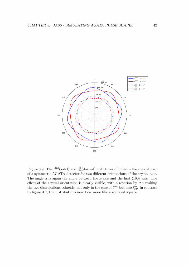
CHAPTER 3. JASS - SIMULATING AGATA PULSE SHAPES 42
100 ns
200 ns
300 ns
400 ns
500 ns
30
210
60
240
90
270
120
300
150
330
180 0
t 100 , α=35°
t 100 , α=80°
t3090, α=35°
t3090, α=80°
Figure 3.9: The t100(solid) and t9030(dashed) drift times of holes in the coaxial partof a symmetric AGATA detector for two different orientations of the crystal axis.The angle α is again the angle between the x-axis and the first 〈100〉 axis. Theeffect of the crystal orientation is clearly visible, with a rotation by ∆α makingthe two distributions coincide, not only in the case of t100 but also t9030. In contrastto figure 3.7, the distributions now look more like a rounded square.

CHAPTER 3. JASS - SIMULATING AGATA PULSE SHAPES 43
times of the holes in solid lines and for t9030 in dashed lines, for interactions locatedat the core contact in the coaxial part of a symmetric AGATA detector. This isequivalent to the electrons being collected immediately and only the holes driftingthrough the detector. The angle α is defined in the same manner as in figure 3.7,and is 35 for the blue curve and 80 for the red curve. As is the case with theelectrons, the anisotropy rotates along with the crystal orientation and a simplerotation by ∆α suffices to make both distributions coincide. In stark contrast tothe electron drift times the anisotropy is now devoid of any oscillations and looksmore like a rounded square or warped circle.
3.3 Calculating the Pulse Shapes
With the trajectories of the charge carriers given from the previous steps, theremaining task is to calculate the signals induced by the charge carriers on eachelectrode of the AGATA detector along their trajectory. Theoretically, one wouldhave to go through the tedious process of solving equation 3.6 for the electricfield with the charge q at ~r(t) and then integrating its normal component overthe surface of the electrode in question for every point on the trajectory. Thishowever can be greatly simplified by use of the Shockley-Ramo theorem.
3.3.1 The Shockley-Ramo Theorem
The Shockley-Ramo theorem was independently discovered by (Shockley, 1938)and (Ramo, 1939). Though it was originally derived for vacuum tubes only, itwas later shown that it still holds under the presence of a stationary space chargedistribution (Jen, 1941; Cavalleri, 1971). A recent review relevant to this thesiscan be found in (He, 2001).The theorem states that, for a set of electrodes 1, . . . , n the charge Qi inducedon electrode i by a moving point charge q at an arbitrary point ~r is given by:
Qi = −q · ψi(~r) (3.20)
The so-called weighting potential ψi(~r) for electrode i is calculated from thePoisson equation with the boundary conditions:
ψ(~r) = 1V ∀~r ∈ ∂Ωi
ψ(~r) = 0V ∀~r ∈ ∂Ωj 6=i (3.21)
with the surface area of electrode i given by ∂Ωi. Additionally, the space chargeρ(~r) is set to zero, hence the induced charge Qi is independent of the appliedelectric field and the space charge, just like the weighting potential(see eqn. 3.20).Figure 3.10 shows a 2D-color plot at y = 0mm of the weighting Potential forsegment A4 of the symmetric prototype. The potential is decaying sharply outside
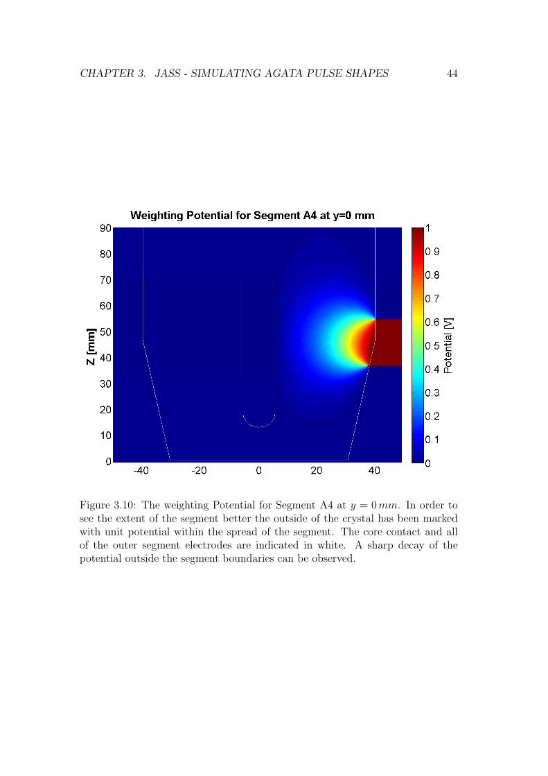
CHAPTER 3. JASS - SIMULATING AGATA PULSE SHAPES 44
Figure 3.10: The weighting Potential for Segment A4 at y = 0mm. In order tosee the extent of the segment better the outside of the crystal has been markedwith unit potential within the spread of the segment. The core contact and allof the outer segment electrodes are indicated in white. A sharp decay of thepotential outside the segment boundaries can be observed.
CHAPTER 3. JASS - SIMULATING AGATA PULSE SHAPES 45
the segment boundaries. To simulate the pulse shapes for AGATA the weightingpotentials for all segments and the core electrode have to be calculated (see sec.3.3.2). The boundary condition for the passivated layer, as given by eqn. 3.10 istaken over unchanged.
3.3.2 Formation of the Pulse Shapes
To fully understand how the pulse shapes are formed only the case of a singleinteraction needs to be discussed. The interaction of a γ-ray with the detectorcreates a certain number of electron-hole pairs3 with the total number of pairsbeing proportional to the energy deposited by the interaction. Once created theresulting charge clouds of charge −q for the electrons and +q for the holes, startdrifting away from the site of the interaction in opposite directions ( see left panelof fig. 3.11). The hole cloud will be collected by the segment electrodes and theelectron cloud by the central contact, as in any n-type germanium detector. Aninteraction is said to have taken place within a given segment if that segmentselectrode is collecting the holes. Along their respective trajectories each typeof charge carrier is inducing a charge on the electrodes according to equation3.20. The overall charge induced at electrode i is then given by the sum for bothtypes of charge carriers and the time dependent charge signal Qi(t) can hence bewritten as:
Qi(t) = q [ψi(−→re (t)) − ψi(
−→rh(t))] . (3.22)
At the end of their trajectory the charge carriers are collected and the position−−→re/h of the electrons or holes is no longer defined since they immediately recombinewith their mirror charges and cause a discontinuous drop in the current signal.The observed charge signals, by contrast show a completely steady behavior (seeright panel of fig. 3.11). This can be understood since the charge signals simplyare the integral of the current signals. In order for a simulation to reproduce theobserved signals correctly the additional assumption has to be made that, oncecollected, the charge carriers are virtually staying at the collecting electrode, con-tinuing to induce a signal as given by the boundary conditions 3.21. This ensuresthat the electrodes will record a constant charge signal4 that is proportional tothe total amount of charge having been collected by each electrode.
These are all the ingredients necessary to understand how the different pulseshapes come about. At the time t0 of the interaction it obviously holds that−→re (t0) = −→rh(t0) and therefore Qi(t0) = 0. In the following the contribution ofthe holes and electrons to the charge signal of segment i is given by the shape of
3An interaction always creates as many holes as electrons. If the detector has been damagedby neutrons charge trapping can occur and this balance is no longer valid. The effect, however,is too small to have an influence on the position resolution (Ljungvall & Nyberg, 2005; Descovichet al., 2005)
4The effects of the electronics response functions will be applied onto these raw signals andexplained in section 3.5
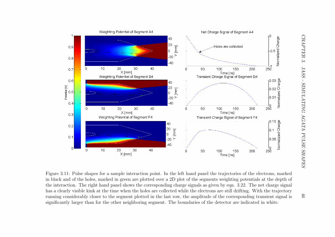
CH
AP
TE
R3.
JA
SS
-SIM
ULA
TIN
GA
GA
TA
PU
LSE
SH
AP
ES
46
Figure 3.11: Pulse shapes for a sample interaction point. In the left hand panel the trajectories of the electrons, markedin black and of the holes, marked in green are plotted over a 2D plot of the segments weighting potentials at the depth ofthe interaction. The right hand panel shows the corresponding charge signals as given by eqn. 3.22. The net charge signalhas a clearly visible kink at the time when the holes are collected while the electrons are still drifting. With the trajectoryrunning considerably closer to the segment plotted in the last row, the amplitude of the corresponding transient signal issignificantly larger than for the other neighboring segment. The boundaries of the detector are indicated in white.

CHAPTER 3. JASS - SIMULATING AGATA PULSE SHAPES 47
the weighting potential ψi along the unique trajectory of the respective chargecarrier (see eqn. 3.22). Segments that were not hit will show only transient charge
signals that return to zero once all charges have been collected. The upper rowin figure 3.11 shows the example of a net charge signal for segment A4 of thesymmetric prototype detector.
As can be seen in the middle and lower plots of figure 3.11 the amplitude ofa transient signal is larger the closer the trajectory runs to the boundary of therespective neighboring segment. The electrodes of the core contact and the hitsegment are therefore the only ones recording net charge signals of opposite sign.Once the holes are collected the shape of the signal depends only on the pathof the electrons through the weighting potential causing a kink in the recordedsignal. Depending on the location the net charge signal can also change curvatureif one type of charge carrier is collected. It is this location dependence that formsthe basis for the pulse shape analysis to retrieve the interaction location from therecorded pulse shapes (see chap. 4).
3.3.3 Interpolation
Since all potentials needed are only available on fixed grid points with finitespacing, a precise interpolation routine marks a cornerstone of any simulation ofpulse shapes. Naturally the accuracy of the interpolation increases with higherinterpolation order R as more and more grid points are included (see fig. 3.12 forthe 2D case) but only for steady functions. Discontinuities, as they are found at
x
yFigure 3.12: For a 0th order interpo-lation only the innermost red pointsare used. The black filled circles areadded for 1st order and the outer-most open circles for 2nd order inter-polation.
the segment boundaries, are smoothed increasingly by higher orders. Also a largeorder would take too long to compute since the simulation needs to interpolate all37 weighting potentials at every point along the trajectories of the test charges.Hence a compromise between accuracy inside the crystal and at the boundariesas well as computation speed has to be found.
Generally speaking an interpolation calculates a weighted sum of the valuesgiven at the used grid points. The weights depend on the distance betweenthe grid point and the point of interpolation and are naturally normalized tounity. (Schonberg, 1946) showed that any interpolation can be written in terms

CHAPTER 3. JASS - SIMULATING AGATA PULSE SHAPES 48
of a kernel-interpolation in which the distance is weighted by the kernel functionF (~r, ~rk).
ψ(~r) =N∑
k=1
F (~r, ~rk) · ψ(~rk) (3.23)
The most simple approach is the trilinear interpolation with a B-Spline of de-gree 1 as the interpolating kernel. It is only used at 0th order since the linearapproximation to the potentials is only justified at the finest grid level.
(Shannon, 1949) showed that the sinc function represents the theoreticallyoptimal choice of a kernel in the case of 1-D band-limited signals. This optimalityalso holds at higher dimensions (see e.g. (Meijering et al., 1999)), but only whenusing an infinite number of lattice points. In order to be able to use it in asimulation and also to counter the effects of the truncation error, the sinc functionneeds to be multiplied with a windowing function of finite extent. The completekernel, using a Hamming window is then given by:
F (~r, ~rk, R) =∏
a=x,y,z
sin (π(a− ak))
2π (a− ak)· (1 + cos (π(a− ak)/(R + 1))) (3.24)
with the already mentioned interpolation order R. Another possible choice forthe kernel is a Gaussian
F (~r, ~rk) =1√
2π · σ2· exp
(
−‖~r − ~rk‖2σ2
)
(3.25)
which according to (Schonberg, 1946) falls into the class of smoothing interpola-tion since then ψ(~rk) 6= ψ(~rk). Yet this kernel is still very attractive for use withequidistant grids. A suitable choice of σ in relation to the grid spacing along withan interpolation order, which includes points within ± 3σ can make the errors ofthe interpolation negligible (Monaghan, 1985).
Figure 3.13 shows the residuals of the three interpolation methods from theknown values of the weighting potential for a true coaxial detector given byeqn. 3.8. The interpolations were conducted along a line inclined 15 degreeswith respect to the x-axis. The trilinear method has by far the largest errorsand also showed a strong dependence on the orientation within the detector. Infact the only time its output had acceptable errors was for interpolations alongone of the axis of the coordinate system. The sinc-interpolation with order twofairs considerably better in terms of errors but suffers from substantial ringing.These oscillations would also be visible in the simulated signal and are thereforeundesirable. Using the Gaussian kernel of the same order produced the expectedsmooth curve and also the smallest errors of all the three methods tested. As anadded advantage its performance was independent of the orientation within thedetector. Going to higher orders has no significant influence on the precision ofeach kernel.

CHAPTER 3. JASS - SIMULATING AGATA PULSE SHAPES 49
5 10 15 20 25 30 35−0.04
−0.02
0
0.02
Re
siu
da
l of K
ern
el I
nte
rpo
latio
ns
[V]
Residuals for a true coaxial detector
5 10 15 20 25 30 35−1
−0.5
0
0.5
Radius [mm]
Re
sid
ua
l of T
rilin
ea
r In
terp
ola
tion
[V
]
Partial SincGauss
Trilinear
Figure 3.13: Residuals from the interpolation of the core weighting potential of atrue coaxial detector as a function of the detector radius. The right abscissa is forthe trilinear interpolation, which has by far the largest errors and the left is for thekernel-based methods. The sinc-interpolation with order two shows considerableringing in contrast to the smooth output achievable by using a Gaussian kernel.

CHAPTER 3. JASS - SIMULATING AGATA PULSE SHAPES 50
Equation 3.22 shows that the interpolated values of the weighting potentialshave direct influence on the simulated pulse shape. For example an interpolationmethod which returns values higher than the actual potential in the stronglyvarying regions near the respective segments boundaries would lead to transientsignals with an absolute amplitude higher than found for any interaction withinthe segment. Hence the PSA algorithm can find a better agreement with theexperimental signal by searching further away from the boundaries, leading to aclustering of the reconstructed positions in the middle of the segments. In thecourse of this work it was found that this is the case when using the second orderGaussian kernel (see fig. 3.14). An adaptive routine with the interpolation orderstarting at the default value of two, but which reduces the order to the nextsmaller level once points from outside the crystal would be included, proves to bebetter suited to the problem of calculating the signals. Figure 3.14 displays the
20 30 40 50 60 70−0.5
0
0.5
1
1.5
Z [mm]
Vo
ltag
e [V
]
Weighting potential of segment A4
20 30 40 50 60 70−0.5
0
0.5Residuals
Z [mm]
Vo
ltag
e [V
]
30 35 40
0
0.1
0.2
0.3
Figure 3.14: The precision of the two Gaussian kernel interpolation methodsalong the outside of the crystal for the weighting potential of segment A4 (seefig. 3.10). The black line in the main plot shows the theoretical values givenby the boundary conditions. The fixed-order method (dash-dotted line) has dif-ficulties reproducing the discontinuities at the segment boundaries. Using theadaptive method (dashed line) reduces the residuals, plotted in the lower panel,considerably. The inset shows a zoomed view of the lower segment boundary.

CHAPTER 3. JASS - SIMULATING AGATA PULSE SHAPES 51
precision of both of the above methods along the outside of the AGATA crystalfor the case of the weighting potential of segment A4 (see fig. 3.10). As de-manded by the boundary conditions to the Poisson equation, the correct solutionhas a discontinuous step from zero to unit potential at the lower segment bound-ary and then jumps back zero potential at the upper boundary. The fixed-orderGaussian kernel interpolation smooths the discontinuities quite strongly leadingto considerably larger residuals, depicted in the lower panel, than with the adap-tive method. While there is still some ringing present around the discontinuitiesfor the latter, the steps at the segment boundaries are much better resolved, afact that is also exemplified in the zoomed view of the lower segment boundaryin the inset of the figure.
Besides the test case of the true coaxial detector (see eqn. 3.8) there is anadditional way to gauge the accuracy of the interpolation routine. With thesegment boundaries having a negligible size the AGATA crystals can safely beconsidered as completely enclosed by the segment and core electrodes. There aretwo important consequences to this:
Ψ(~r) =∑
i
ψi(~r) = 1 (3.26)
Qtot(t) =∑
i
Qi(t) = 0 (3.27)
When looking at the sum of all weighting potentials the volume of the detectoris surrounded by electrodes on unit potential. In the absence of any space chargethis means that at each point within the detector the weighting potentials ofall the segments and the core add up to unity. Equation 3.27 implies that thesignal seen by the core contact is equal to the inverse sum of the segment signalsand is a direct consequence of equations 3.26 and 3.22. Not surprisingly the firstcondition does hold on the calculated grid points but it should also hold at off-grid points using only interpolated values for the potentials. For this purpose thetwo fixed-size kernels and the adaptive-sized kernel were used to interpolate allweighting potentials at 100000 randomly distributed points within the detector.The results in table 3.1 again show that both Gaussian kernels are close to the
Kernel Mean Sum [V] Standard Deviation [V]
2nd Order Partial Sinc 0.5404 0.15232nd Order Gaussian 0.9984 0.0139Adaptive Gaussian 1.0007 0.0094
Table 3.1: The sum of all weighting potentials interpolated at off-grid points.
theoretic optimum, while the partial-sinc interpolation is less favorable. Usingan adaptive interpolation order yet again trumps the fixed-size kernels with notonly the mean sum being closest to unity but also having the smallest standard
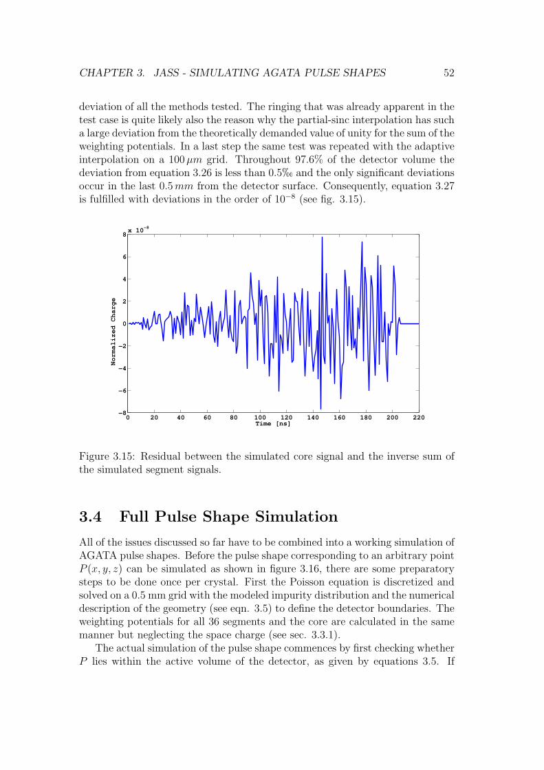
CHAPTER 3. JASS - SIMULATING AGATA PULSE SHAPES 52
deviation of all the methods tested. The ringing that was already apparent in thetest case is quite likely also the reason why the partial-sinc interpolation has sucha large deviation from the theoretically demanded value of unity for the sum of theweighting potentials. In a last step the same test was repeated with the adaptiveinterpolation on a 100µm grid. Throughout 97.6% of the detector volume thedeviation from equation 3.26 is less than 0.5h and the only significant deviationsoccur in the last 0.5mm from the detector surface. Consequently, equation 3.27is fulfilled with deviations in the order of 10−8 (see fig. 3.15).
0 20 40 60 80 100 120 140 160 180 200 220−8
−6
−4
−2
0
2
4
6
8x 10
−8
Time [ns]
No
rma
lize
d C
ha
rge
Figure 3.15: Residual between the simulated core signal and the inverse sum ofthe simulated segment signals.
3.4 Full Pulse Shape Simulation
All of the issues discussed so far have to be combined into a working simulation ofAGATA pulse shapes. Before the pulse shape corresponding to an arbitrary pointP (x, y, z) can be simulated as shown in figure 3.16, there are some preparatorysteps to be done once per crystal. First the Poisson equation is discretized andsolved on a 0.5 mm grid with the modeled impurity distribution and the numericaldescription of the geometry (see eqn. 3.5) to define the detector boundaries. Theweighting potentials for all 36 segments and the core are calculated in the samemanner but neglecting the space charge (see sec. 3.3.1).
The actual simulation of the pulse shape commences by first checking whetherP lies within the active volume of the detector, as given by equations 3.5. If

CHAPTER 3. JASS - SIMULATING AGATA PULSE SHAPES 53
that is the case the electric field at the initial position is interpolated from thevalues of the electric potential. The charge carriers positions are then advancedaccordingly, using the mobility models described in sections 3.2.3 and 3.2.4 andtime steps of 0.1ns to discretize the equation of motion. These new position arethen checked again with the detector boundaries. This is repeated, independentlyfor the electrons and the holes, until the new position is found to be outside theactive volume. The small time step ensures that the charge carrier is stoppedwithin 10µm of the actual detector boundary and also prevents the oscillationsaround the correct path observed with larger time steps. Once both the holes aswell as the electrons have reached the collecting electrodes the calculation stopsand the trajectory has been fully calculated.
Since the pulse shapes need not be available in the high time precision asthe trajectory, due to the 100MHz sampling of the digitizers (see sec. F.2), itsuffices to calculate the signals only for every 10th point on the trajectory, e.g.every 1ns. Starting at P and with the time t set to zero the following steps arerepeated for each of the 36 segments and the core individually:
• Interpolate the weighting potential at the charge carriers position.
• Calculate signal at time t using equation 3.22.
• Advance t by 1ns and update the positions.
• Stop once the holes as well as the electrons have reached their endpoint.
The weighting potential at the endpoint of a trajectory is not interpolated, butthe values demanded by the boundary conditions in equations 3.21 are used. Inthe most common case of different drift times for the electrons and holes, thecharge carrier, which has already reached its endpoint is considered to stay atthat position conserving its contribution to the charge signal (see 3.3.2).
3.5 Response Functions
The basic approach to AGATA PSA is a direct comparison between simulatedand experimental signals (see chap. 4). However, the signal recorded by thedigitizers is not just an amplified version of the original signal shape from thedetector, as it is simulated, but is altered in two ways. First, like any measuringsystem the AGATA readout electronics have a unique response function alteringthe input signal in a defined way. Secondly, although great care has been used inthe cabling of the detector capsules the remaining capacitive coupling betweenany of the segments, or between the core and a segment, still leads to crosstalkeffects between the individual signals. Both effects have to be applied to thesimulated signals before they can be compared with an experimental trace. Inthe following these two influences on the signal shape will be discussed in moredetail.

CHAPTER 3. JASS - SIMULATING AGATA PULSE SHAPES 54
Interaction at P (x, y, z)
check
positionABORT
interpolate
elec. fielddrift holes
check
hole pos.
keep hole
pos.
drift
electrons
check
e− pos.
keep
electron
pos.
calculated trajectory
interpolate
weighting
pot. for h
interpolate
weighting
pot. for e−
calculated signal
no
yes
no
yes
no
yes
Figure 3.16: The principal work flow of JASS. The first check performed testswhether the point P is within the detectors boundaries. Then the pre-calculatedelectric potential is interpolated at the given position and the electrons and holesare drifted, independent of one another, according to their mobility models. Oncea charge carriers reaches the detector boundary it is stopped and its position keptconstant. The calculation of the trajectory is finished if both carriers have reacheda boundary. From this the charge signal Q(t) is computed, repeating those partsframed by the dashed rectangle 37 times, once for each of the 36 segments andthe core.

CHAPTER 3. JASS - SIMULATING AGATA PULSE SHAPES 55
3.5.1 Front End Electronics
The influence of a measuring systems response function H(t), given in the timedomain, on the recorded output signal S(t) can be described by a convolution ofthe input signal I(t) with H(t):
S(t) = (H ∗ I) =
∫ ∞
−∞
H(u) · I(t− u) du. (3.28)
Each single stage of the readout electronics has its own response function, deter-mined by its components, resulting in a nested set of convolutions which moreoften than not cannot be solved analytically. Additionally, determining eachsingle response function is a far from trivial task and not the topic of this the-sis. Therefore only the most important effects, in terms of signal shape, will bediscussed.
The most simple contribution to the signal shape is the discharging of thecapacitance in the charge loop of the preamplifier (see fig. F.1) leading to anexponential decay of the recorded charge signal. The decay time constant of 50µsis given by the values of the resistor and capacitance. This is the only part of theresponse function which can be inverted analytically and deconvolved, removingits effects on the signal shape. Also the charge loop cannot react instantaneouslyto an input but has a finite bandwidth. Thus the rise time of the preamplifier,i.e. the time it takes the preamplifier to reach its maximal output for a stepfunction input, is not zero but finite. In the case of the AGATA preamplifiers therise time can be adjusted within a predefined range and typically is of the orderof 30ns.
The last component in the readout chain with a simple response function isthe Anti-aliasing filter, applied just before the flash ADCs which digitize the sig-nals. According to the Shannon sampling theorem (Shannon, 1949) the 100MHzsampling rate of the digitizers suffice to resolve only contributions with frequen-cies below half the sampling rate. Hence, the anti-aliasing filter acts similar toa low pass filter with a cutoff frequency of 50MHz. Figure 3.17 shows the fre-quency gain of the output signal in dB for a preamplifier with 30ns rise time,an anti-aliasing filter with a cut off frequency of 50MHz and the combined re-sponse. The complete response function in the time domain is plotted in figure3.18(a) and appears to be positively skewed with a non-Gaussian shape to theleft of the peak. The effects of the response function on the signal shape areillustrated in figure 3.18(b) and show a delayed start of the convolved signal withrespect to the raw detector signal and generally a strong smoothing of the pulseshape. The only discernible effect of the exponential decay is in the non-constantcharge signal after all charge has been collected. The analytic deconvolution ofthe latter effect guarantees a proper normalization of the experimental signals tounit charge.
Experimentally it is possible to determine the complete response function R(t)
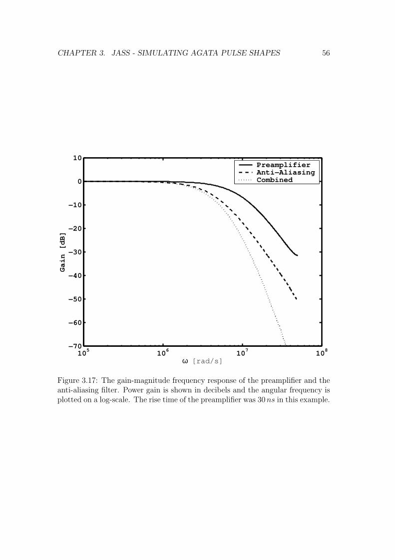
CHAPTER 3. JASS - SIMULATING AGATA PULSE SHAPES 56
105
106
107
108
−70
−60
−50
−40
−30
−20
−10
0
10
ω [rad/s]
Ga
in [d
B]
PreamplifierAnti−AliasingCombined
Figure 3.17: The gain-magnitude frequency response of the preamplifier and theanti-aliasing filter. Power gain is shown in decibels and the angular frequency isplotted on a log-scale. The rise time of the preamplifier was 30ns in this example.

CHAPTER 3. JASS - SIMULATING AGATA PULSE SHAPES 57
0 1 2 3 4 5 6
x 10−7
0
0.01
0.02
0.03
0.04
0.05
0.06
Time [ns]
(a) Response function in the time domian.
0 1 2 3 4 5 6
x 10−7
0
0.2
0.4
0.6
0.8
1
Time[ns]
No
rma
lize
d C
ha
rge
Measured Signal
Raw Signal
(b) Comparison of raw and convoluted, i.e. measured signal.
Figure 3.18: The plot in (a) shows the response function in the time domain andthe effects of the response function on the signal shape are illustrated in (b) Mostnotably the start of the convolved signal (blue) is delayed with respect to the rawdetector signal (red) and the pronounced kink is smoothed rather strongly.
CHAPTER 3. JASS - SIMULATING AGATA PULSE SHAPES 58
using the core pulser (see sec. F.1) to inject a step function signal Θ(t). Thederivative of the recorded signal S(t) is then equal to R(t) as given by
∂
∂tS(t) =
∂
∂t(Θ(t) ∗R(t)) = (
∂Θ(t)
∂t∗R(t)) = (δ(t) ∗R(t)) = R(t), (3.29)
with δ(t) the Dirac delta function. As for the scanning data, the complete re-sponse R(t) of the used readout electronics can be approximated by a Gaussianwith standard deviation σ = 15ns. This covers all characteristics of R(t), in-cluding its finite bandwidth and the frequency limiting of the anti-aliasing filter,except the exponential decay given by the cold part of the preamplifier (Bruyneel,2007).
3.5.2 Crosstalk
Another signal alteration, inherent to any segmented detector, is the so-calledcrosstalk due to capacitive coupling between the detectors electrodes. Two typesof crosstalk can be discerned. Proportional crosstalk is directly proportional tothe signal amplitude while derivative crosstalk is proportional to the derivativeof the signal. The latter contributes only during the rise time of the signal sincethe derivative is zero anytime else.
Proportional Crosstalk
The origin of the proportional crosstalk lies in the capacitive coupling between thedetectors electrodes. The current generated on electrode i will not go in its entityto preamplifier i but parts will be split of by capacitive coupling to electrode jwith the amount proportional to the ratio of the electrodes capacities. However,due to the different coupling of the segment preamplifiers to the detector thesegment to segment and segment to core crosstalk contributions are at least oneorder of magnitude smaller than the core to segment crosstalk (Bruyneel et al.,2009). Consequently only the latter effect will be applied to the simulated signals.It can be implemented by simply adding a scaled copy of the core electrodes chargesignal onto all segment charge signals. For the AGATA detectors the scalingfactor is 0.1% (Bruyneel et al., 2009), in line with the AGATA specifications. Itspredominant effect is a shift in the segment signals base line leading to reductionof the energy detected by the segment. Thus the sum of segment energies, whichideally should be equal to the core energy, is reduced around 0.1% per segmentfold5 (see fig. 3.19(b)).
5Segment fold or multiplicity denotes the number of segments with a γ-ray interaction, i.e.a net charge signal.

CHAPTER 3. JASS - SIMULATING AGATA PULSE SHAPES 59
0 50 100 150 200 250 300−0.02
0
0.02
0.04
0.06
0.08
0.1
0.12
Time [ns]
No
rma
lize
d C
ha
rge
no crosstalkproportionalproportional+derivative
Base line shift
(a) Effects of both crosstalk contributions on a transient signal. The effects have been exaggeratedfor an enhanced clarity of the figure.
(b) The sum of segment energies as a function of segment fold.
Figure 3.19: Illustration of crosstalk effects on signal shape (a) and energy res-olution (b). The proportional core to segment crosstalk(exaggerated by a factorof 10, red, a) leads to a shift of all segment base lines and reduces the energydetected by the segment. The sum of segment energies decreases linearly withincreasing segment fold (b) (fig. taken from (Bruyneel et al., 2009)). The sig-nal shape is predominantly influenced by the derivative crosstalk (exaggerated 4times, green, a) component with a significant change in recorded signal ampli-tude. The proportional crosstalk by the core affects the signal shape only in thelater stages, for instance from t90 onward.
CHAPTER 3. JASS - SIMULATING AGATA PULSE SHAPES 60
Derivative Crosstalk
Derivative crosstalk is proportional to the derivative of the induced net chargesignal and contributes to the signal shape only during the rise time of the signal,i.e. the region of interest for PSA (see chap. 4). Only the directly neighboringsegments and and segments within the same sector are affected by this type ofcrosstalk (Dimmock, 2008), which are exactly the segments used by PSA. Theshape of the resulting crosstalk signal is similar to that of transient signals, mak-ing it rather hard to measure precisely in experimental signals, and has a signifi-cant influence on the amplitude of a transient signal (see fig. 3.19(a)). Thereforeit would be of great importance to PSA to include the effect but unfortunatelythere is not yet a measurement of derivative crosstalk for any AGATA crystalsince it requires time aligned signals. This was not possible with the electronicsused in the scanning of the detector (see sec. 3.6.1) and the effect could not beincluded in the simulated signals.
3.6 Verification of JASS with experimental data
The verification of the simulated pulse shapes is absolutely essential before sim-ulated traces can be used to perform a pulse shape analysis of experimentaldata with unknown interaction locations. Any inaccuracies of the simulationwould have a direct impact on the accessible position resolution of the PSAand hence on the precision of the tracking algorithms ultimately affecting theDoppler-correction capabilities.
There are two principal ways to achieve a full or partial verification. First ofall a collimated source, with a so-called pencil beam, can be placed in front of thedetector and the reconstructed interaction locations should show the expectedexponential distribution with depth. The particular problem with this approachlies in the fact that the majority of events will have multiple γ-ray interactions inthe crystal. These have to be decomposed correctly in order for the result to becomparable with the theoretical expectations. These approach will not be takenin this thesis, due to the additional error sources on the PSA side that preventa proper evaluation of the accuracy of the simulation. The second possibilityis to use a coincidence scan setup, where all three coordinates of an interactionare simply given by the setup of the experiment (see sec. 3.6.1) and the vastmajority of event will be single γ-ray interactions (see tab. 3.2). If the positionsfrom various scan points are correctly identified by a full search of the simulateddataset the simulation can be considered verified and this is the approach takenin this thesis.
The comparison of the experimental traces with data simulated by JASSwas conducted in the following manner. First a signal basis with a grid sizeof 1 mm was calculated by JASS, using in one case the mobility parameters

CHAPTER 3. JASS - SIMULATING AGATA PULSE SHAPES 61
reported by (Bruyneel, 2007), this will be called parameters set A in the following.Additionally, the electron mobility parameters from (Mihailescu et al., 2000) inconjunction with the hole mobility parameters for the presented model (see sec.3.2.4), which were adjusted to the experimental results from (Reggiani et al.,1977) by (Bruyneel et al., 2006a) were used, this will be called parameter setB in the following. For a description of the model parameterization and therespective parameters the reader is referred to appendix B. Next these pulseshapes were folded with the response function as pointed out in section 3.5 andthe proportional core-to-segment crosstalk was added. Using these simulatedsignal bases, an extensive grid search was conducted for each basis, comparingthe experimental traces with each pulse shape from the basis and the coordinatesof the best fitting trace were recorded. Naturally only basis points within thehit segment were considered and the comparison only used the transients of thesegments directly adjacent to the hit segment in addition to the net charge signal.Given the amplitude of transients from segments further away, including thesewould only have a negligible influence on the overall value of the metric. Sincethere was no real-time requirement in this setting, the starting time t0 of thepulse shapes was kept as a fit parameter and only the optimized value of themetric entered the comparison with the other basis points.
3.6.1 Comparison with Scanning Data of S002
The basic idea of the scanning system is to use the AGATA detector togetherwith an ancillary detector, e.g. scintillators, to selectively measure only eventsin which the γ-ray Compton-scattered by 90, with the ancillary setup fixingthe z position of the interaction within the AGATA detector. The experimentalwork of the coincidence scan and the setup were done by Matthew R. Dimmockand Laura Nelson, a detailed description of the scanning setup can be found in(Dimmock, 2008). The basic parts for this work are summarized in the following.
A 920 MBq 137Cs source was placed inside a lead block, which had a borehole with 1 cm diameter located just above the source. This block was fittedonto a motorized x-y-table to allow for a precise positioning of the source and a1 mm wide collimator was placed in front of the source to constrain the x andy position. The z position is determined by the ancillary detector, either NaIor BGO crystals, which detected a γ-ray in coincidence with AGATA as eachdetector covers just one collimated slit between adjacent semi-circular sheets oflead placed around the AGATA crystal. The complete setup up is illustratedin figure 3.20. The event selection procedure sorted out all events in which theenergies deposited in the AGATA detector and the scintillators did not matchthose required for a 90 Compton-scattering of a 662 keV γ-ray. Additionally,allowances for the energy resolutions of the detectors were made and only eventsin which just one AGATA segment recorded an interaction were accepted. Usingthis setup, shown in figure 3.20, the x and y positions of an interaction are known

CHAPTER 3. JASS - SIMULATING AGATA PULSE SHAPES 62
Figure 3.20: Illustration of the setup of the Liverpool scanning system showingthe positioning of the various components. The slits forming the collimators forthe z-position of the γ-ray interaction have different widths of 1.5mm and 3.0mmin order to allow for similar amounts of events to be recorded for each scanneddepth. The positions of the slits were chosen in such a way as not to cover twodifferent effective segment rows, indicated by lines in the crystal, with the samecollimators. The figure was taken from (Dimmock, 2008).

CHAPTER 3. JASS - SIMULATING AGATA PULSE SHAPES 63
from the x-y-table and the z position is given by the scintillator, which detectedthe scattered γ-ray. The pulse shapes from the AGATA detector were read outby GRT4 cards (Lazarus et al., 2004), that were not time aligned, and with asampling rate of 80MHz. The time alignment of the segment shapes happenedlater in a post-processing step (for details see (Dimmock, 2008)). It should benoted that a better quality of the data can be expected when using the fullAGATA electronics (see sec. 2.2).
The raw data from the scan consisted of non-normalized traces with 250 sam-ples for each segment trace, in need for some preprocessing before a comparisonwith the simulated data could proceed. The data was already arranged in sucha manner that the starting time t0 of the pulses was always in the vicinity ofsample 100. In a first step the known exponential decay from the preamplifierwas removed from the traces by analytic deconvolution. Next the baseline of thepulse shapes was adjusted by calculating the average value of the first 80 samplesand subsequent subtraction of it. In a last step the traces had to be normalizedto the hit segment having unit charge. Therefore all traces were divided by theaverage of the samples 170 through 250 of the hit segment. Sample 170 is 875 nsaway from the typical starting sample 100 and hence has a large enough safetymargin to not include parts of the rising pulse since the longest drift times are ofthe order of 350 ns.
Position uncertainties of the setup
In order to be able to gauge the precision of JASS it is necessary to know thesystematic position uncertainties, as given by the setup of the scanning system.For this purpose a GEANT simulation was conducted, using a reduced setup con-taining only two slits. The first slit was situated at a depth of 31mm within thedetector and had an extent of 1.5mm, while the second one was 3mm wide andat a depth of 80mm. Additionally it was assumed that the slits are completelycovered by two NaI scintillators, affecting only the statistics but not the precisionof the setup. Out of the one billion γ’s simulated in total, those fulfilling the cri-terion of a coincident 90 Compton scattering have to be extracted. A 662 keV γshould hence deposit 374 keV in the AGATA crystal and 288 keV in the scintil-lators. Due to the limited energy resolution of any detector only finite intervalsaround the correct energies can be used. Even though the intrinsic resolution ofAGATA is 1.5 keV (FWHM) in the relevant energy regime, the applied intervalis 30 keV wide to account for the limited acceptance angle of the geometry. Theenergy gate for the scintillators had to be chosen rather large with a width of150 keV , because of problems with the data acquisition (Unsworth, 2009). Thelatter has no significant influence on the results since the energy gate on theAGATA detectors constrains the energy of the outgoing γ such that it is alwayswithin the given window, even when the effect of the scintillators’ poor energyresolution is included. In addition the energy deposits in the AGATA crystal

CHAPTER 3. JASS - SIMULATING AGATA PULSE SHAPES 64
have to be constraint to a single segment. After this event selection merely 29000γ’s remain.
Figure 3.21(a) shows a scatterplot of the x and y coordinates of the γ-raysmost energetic interaction with AGATA. There is a clear concentration aroundthe source position, indicated by the white cross, but positions outside the areacovered by the opening angle of the collimator are observed as well. These corre-spond to events with multiple γ-interactions and the first interaction not deposit-ing the most energy. As can be seen in figure 3.21(b) a 3mm wide slit does notconstrain the z position of an interaction very well. The distribution is basicallyuniform over the extent of the slit.
The complete results of this simulation are summarized in table 3.2. Thex and y coordinates are precisely constraint by the setup, though the FWHMnaturally increases with depth in the detector due to the finite opening angle ofthe collimator. (Dimmock, 2008) derived similar results, including the uncertain-ties of the source position, with a FWHM of 1.5mm at z = 0 and 3.0mm atz = 90. The picture looks quite different concerning the depth, or z coordinate,of the interaction. Although the source is located rather close to the outside ata radius of 24mm, and hence close to the collimator, its location is not very wellconstraint. The positional errors almost double when using the wider collima-tor of 3mm. Additionally for source position closer to the core, at radii shortlyabove 5mm, the errors will increase because of the opening angle of the relevantcollimator. Also the finite width of the energy intervals do not only allow for
Scanning depth [mm] ∆X [mm] ∆Y [mm] ∆Z [mm]
31 1.3 1.3 2.280 1.6 1.6 4.2
Numb. of Inter. 1 2 3 4Percentage 86% 5.8% 1.8% 5.3%
Table 3.2: The position uncertainties of the scanning setup for the two differenttested depth given as FWHM. The precision in x and y is generally quite goodand decreases with depth due to the opening angle of the collimator. The zcoordinate is by comparison rather poorly constraint by the setup.
scattering angles between 85.5 and 95.5, but also for multiple interactions topass the event selection. Therefore only 86% of the events are single interactionsopposed to the 100% in the ideal case of solely 90 scattering being allowed. maxat 4 phase space.
As the signal shapes vary non-linearly with location ( see fig. 4.1) and with asignificant number of events featuring multiple γ-interactions within AGATA, anaveraging procedure to reduce the influence of noise would not properly reproducethe shape of the mean position of all events. For this reason the decision wastaken to use the scanning data event by event instead of one averaged pulse per
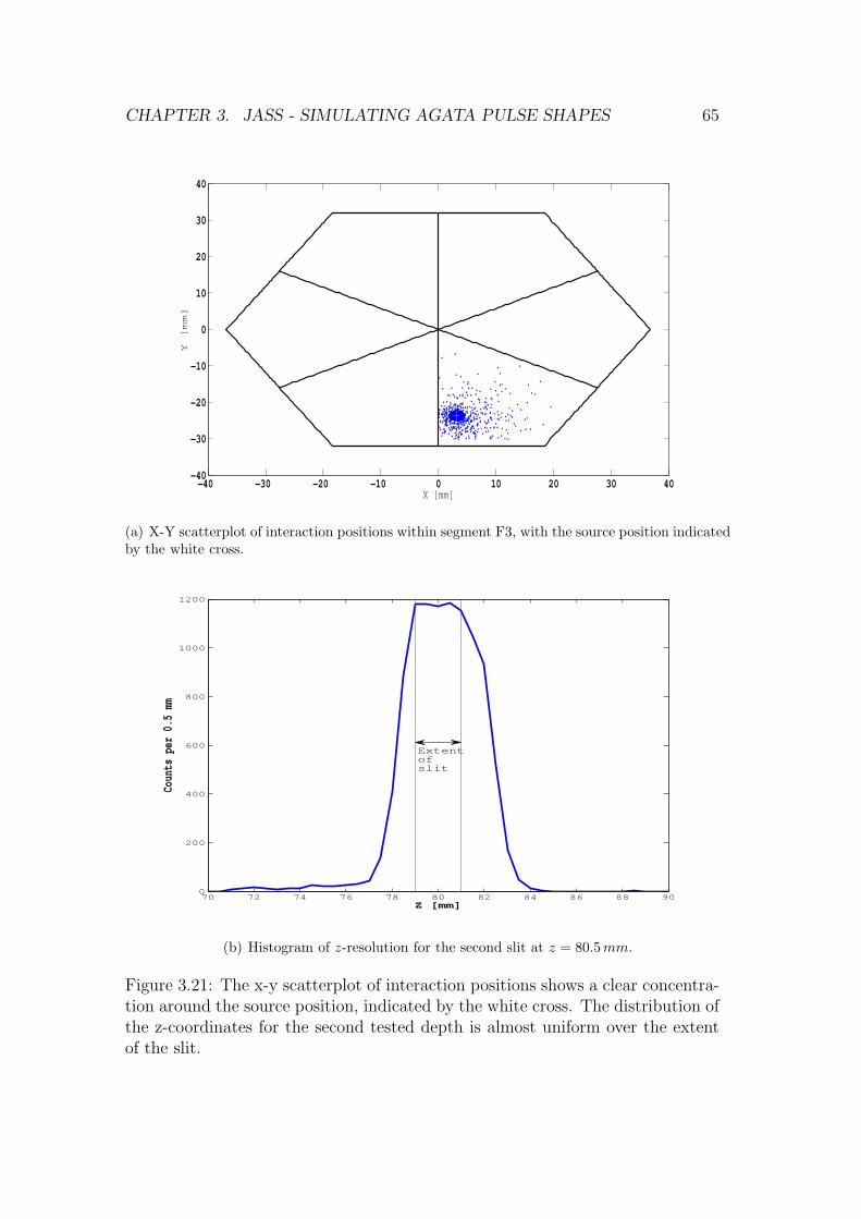
CHAPTER 3. JASS - SIMULATING AGATA PULSE SHAPES 65
−40 −30 −20 −10 0 10 20 30 40−40
−30
−20
−10
0
10
20
30
40
X [mm]
Y [m
m]
(a) X-Y scatterplot of interaction positions within segment F3, with the source position indicatedby the white cross.
70 72 74 76 78 80 82 84 86 88 900
200
400
600
800
1000
1200
Z [mm]
Coun
ts p
er 0
.5 m
m
Extent of slit
(b) Histogram of z-resolution for the second slit at z = 80.5mm.
Figure 3.21: The x-y scatterplot of interaction positions shows a clear concentra-tion around the source position, indicated by the white cross. The distribution ofthe z-coordinates for the second tested depth is almost uniform over the extentof the slit.

CHAPTER 3. JASS - SIMULATING AGATA PULSE SHAPES 66
scanning position.
Single event data
As was already mentioned the preprocessing of the data consisted of an analyticdeconvolution of the exponential decay, given by the preamplifier, and a nor-malization of the net charge signal to unit charge. Additionally, the scanningpositions had to be corrected for a tilt and rotation of the detector (see (Dim-mock, 2008)). In order to verify JASS with this data set a basis set of pulseshapes was simulated on a 1 mm grid, using parameter sets A and B and the pa-rameterization of the charge carrier mobility models presented in appendix B. Acomplete search of all reference signal, including the crosstalk contribution fromthe core signal (see sec. 3.5.2), in the hit segment was conducted to find the basissignal which best agrees with the experimental signal. The event time t0 (see fig.4.3) was a fit parameter and individually optimized for each reference signal. Forthis purpose each reference signal was subsampled to 12.5ns, i.e. the samplingtime of the experimental data, with t0 being varied in 1ns steps over a wideenough range to guarantee the inclusion of the correct t0. Any signal values atsample times without a directly corresponding value in the reference signal, givenwith 1ns precision, were interpolated linearly. Only the best χ2-value from thet0 fit is used in the comparison with the results of the other reference signals andthe grid point with the best overall χ2 is considered the solution to the search.The uncertainties of the setup (see above) and the non-linearities of the signalshapes prevent a complete assessment of JASS’ performance solely based on thesespectra. Therefore pulse shapes from a GEANT simulated set of single interac-tions throughout the detector were calculated, realistic noise (see sec. 4.1) of thecorrect amplitude was added to the signals and the resulting data set was ana-lyzed in the same manner as the scanning data. Before the position resolutions(dashed red curves in figs. 3.22 through 3.28) were calculated the true interactionlocations were smeared by sampling from the position uncertainty distributions,presented in the previous section.
(Bruyneel, 2007) and (Dimmock, 2008) already reported that the scanningdepth are offset by ∼ 4mm, thus this offset has been included in the calculatedspectra and should in principle lead to a peaking of the resolutions in Z around0, just like the distributions of the simulated data set. Figures 3.22 through 3.27show the resolutions for the six different segment rows and figure 3.28 shows theresolution of the complete data set with the blue curves corresponding to theresults of the scanning data with parameter set A, the dash-dotted green curvescorrespond to the results with parameter set B and the dashed red curves be-longing to the results with the simulated data set, i.e. the best possible results.Generally the results can be summarized as follows, the distributions of the X,Yand Z coordinates always have a skewness (see app. E.2) around 0 indicatingsymmetric distributions around the mean. The same is true for the radial coordi-

CHAPTER 3. JASS - SIMULATING AGATA PULSE SHAPES 67
−15 −10 −5 0 5 10 150
2000
4000
6000
8000
10000
12000
Xf − X
true [mm]
Co
un
ts p
er
mm
(a) Resolution of X.
−15 −10 −5 0 5 10 150
1000
2000
3000
4000
5000
6000
7000
8000
9000
10000
Yf − Y
true [mm]
Co
un
ts p
er
mm
(b) Resolution of Y .
−15 −10 −5 0 5 10 150
0.5
1
1.5
2
2.5x 10
4
Zf − Z
true [mm]
Co
un
ts p
er
mm
(c) Resolution of Z.
−15 −10 −5 0 5 10 150
1000
2000
3000
4000
5000
6000
7000
8000
9000
Rf − R
true [mm]
Cou
nts
per m
m
(d) Resolution of R.
−30 −20 −10 0 10 20 300
500
1000
1500
2000
2500
3000
3500
4000
4500
φf − φ
true [deg]
Cou
nts
per d
eg
(e) Resolution of ϕ.
Figure 3.22: Resolutions of scanning events in segment row 1. The blue curveshows the resolution on the scanning data using parameter set A, the dash-dotted green curve belongs to parameter set B and the dashed red curve showsthe resolution on the simulated data.

CHAPTER 3. JASS - SIMULATING AGATA PULSE SHAPES 68
−15 −10 −5 0 5 10 150
500
1000
1500
2000
2500
3000
3500
4000
Xf − X
true [mm]
Co
un
ts p
er
mm
(a) Resolution of X.
−15 −10 −5 0 5 10 150
500
1000
1500
2000
2500
3000
3500
4000
Yf − Y
true [mm]
Co
un
ts p
er
mm
(b) Resolution of Y .
−15 −10 −5 0 5 10 150
500
1000
1500
2000
2500
3000
3500
4000
Zf − Z
true [mm]
Co
un
ts p
er
mm
(c) Resolution of Z.
−15 −10 −5 0 5 10 150
500
1000
1500
2000
2500
3000
3500
4000
4500
5000
Rf − R
true [mm]
Cou
nts
per m
m
(d) Resolution of R.
−30 −20 −10 0 10 20 300
200
400
600
800
1000
1200
1400
φf − φ
true [deg]
Cou
nts
per d
eg
(e) Resolution of ϕ.
Figure 3.23: Resolutions of scanning events in segment row 2. The blue curveshows the resolution on the scanning data using parameter set A, the dash-dotted green curve belongs to parameter set B and the dashed red curve showsthe resolution on the simulated data.

CHAPTER 3. JASS - SIMULATING AGATA PULSE SHAPES 69
−15 −10 −5 0 5 10 150
1000
2000
3000
4000
5000
6000
7000
8000
Xf − X
true [mm]
Co
un
ts p
er
mm
(a) Resolution of X.
−15 −10 −5 0 5 10 150
1000
2000
3000
4000
5000
6000
7000
Yf − Y
true [mm]
Co
un
ts p
er
mm
(b) Resolution of Y .
−15 −10 −5 0 5 10 150
1000
2000
3000
4000
5000
6000
7000
8000
9000
10000
Zf − Z
true [mm]
Co
un
ts p
er
mm
(c) Resolution of Z.
−15 −10 −5 0 5 10 150
2000
4000
6000
8000
10000
12000
Rf − R
true [mm]
Cou
nts
per m
m
(d) Resolution of R.
−30 −20 −10 0 10 20 300
500
1000
1500
2000
2500
3000
3500
φf − φ
true [deg]
Cou
nts
per d
eg
(e) Resolution of ϕ.
Figure 3.24: Resolutions of scanning events in segment row 3. The blue curveshows the resolution on the scanning data using parameter set A, the dash-dotted green curve belongs to parameter set B and the dashed red curve showsthe resolution on the simulated data.
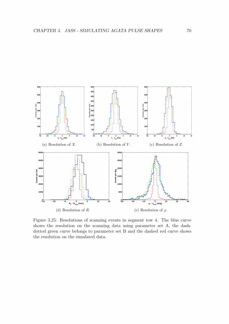
CHAPTER 3. JASS - SIMULATING AGATA PULSE SHAPES 70
−15 −10 −5 0 5 10 150
1000
2000
3000
4000
5000
6000
Xf − X
true [mm]
Co
un
ts p
er
mm
(a) Resolution of X.
−15 −10 −5 0 5 10 150
500
1000
1500
2000
2500
3000
3500
4000
4500
5000
Yf − Y
true [mm]
Co
un
ts p
er
mm
(b) Resolution of Y .
−15 −10 −5 0 5 10 150
1000
2000
3000
4000
5000
6000
Zf − Z
true [mm]
Co
un
ts p
er
mm
(c) Resolution of Z.
−15 −10 −5 0 5 10 150
1000
2000
3000
4000
5000
6000
Rf − R
true [mm]
Cou
nts
per m
m
(d) Resolution of R.
−30 −20 −10 0 10 20 300
500
1000
1500
2000
2500
3000
φf − φ
true [deg]
Cou
nts
per d
eg
(e) Resolution of ϕ.
Figure 3.25: Resolutions of scanning events in segment row 4. The blue curveshows the resolution on the scanning data using parameter set A, the dash-dotted green curve belongs to parameter set B and the dashed red curve showsthe resolution on the simulated data.

CHAPTER 3. JASS - SIMULATING AGATA PULSE SHAPES 71
−15 −10 −5 0 5 10 150
100
200
300
400
500
600
700
Xf − X
true [mm]
Co
un
ts p
er
mm
(a) Resolution of X.
−15 −10 −5 0 5 10 150
100
200
300
400
500
600
700
Yf − Y
true [mm]
Co
un
ts p
er
mm
(b) Resolution of Y .
−15 −10 −5 0 5 10 150
100
200
300
400
500
600
700
800
Zf − Z
true [mm]
Co
un
ts p
er
mm
(c) Resolution of Z.
−15 −10 −5 0 5 10 150
100
200
300
400
500
600
700
800
900
Rf − R
true [mm]
Cou
nts
per m
m
(d) Resolution of R.
−30 −20 −10 0 10 20 300
50
100
150
200
250
300
φf − φ
true [deg]
Cou
nts
per d
eg
(e) Resolution of ϕ.
Figure 3.26: Resolutions of scanning events in segment row 5. The blue curveshows the resolution on the scanning data using parameter set A, the dash-dotted green curve belongs to parameter set B and the dashed red curve showsthe resolution on the simulated data.

CHAPTER 3. JASS - SIMULATING AGATA PULSE SHAPES 72
−15 −10 −5 0 5 10 150
200
400
600
800
1000
1200
Xf − X
true [mm]
Co
un
ts p
er
mm
(a) Resolution of X.
−15 −10 −5 0 5 10 150
200
400
600
800
1000
1200
Yf − Y
true [mm]
Co
un
ts p
er
mm
(b) Resolution of Y .
−15 −10 −5 0 5 10 150
100
200
300
400
500
600
700
Zf − Z
true [mm]
Co
un
ts p
er
mm
(c) Resolution of Z.
−15 −10 −5 0 5 10 150
200
400
600
800
1000
1200
1400
Rf − R
true [mm]
Cou
nts
per m
m
(d) Resolution of R.
−30 −20 −10 0 10 20 300
100
200
300
400
500
600
φf − φ
true [deg]
Cou
nts
per d
eg
(e) Resolution of ϕ.
Figure 3.27: Resolutions of scanning events in segment row 6. The blue curveshows the resolution on the scanning data using parameter set A, the dash-dotted green curve belongs to parameter set B and the dashed red curve showsthe resolution on the simulated data.

CHAPTER 3. JASS - SIMULATING AGATA PULSE SHAPES 73
−15 −10 −5 0 5 10 150
0.5
1
1.5
2
2.5
3x 10
4
Xf − X
true [mm]
Cou
nts
per m
m
(a) Resolution of X.
−15 −10 −5 0 5 10 150
0.5
1
1.5
2
2.5
3x 10
4
Yf − Y
true [mm]
Cou
nts
per m
m
(b) Resolution of Y .
−15 −10 −5 0 5 10 150
0.5
1
1.5
2
2.5
3
3.5
4x 10
4
Zf − Z
true [mm]
Cou
nts
per m
m
(c) Resolution of Z.
−15 −10 −5 0 5 10 150
0.5
1
1.5
2
2.5
3
3.5x 10
4
Rf − R
true [mm]
Cou
nts
per m
m
(d) Resolution of R.
−30 −20 −10 0 10 20 300
2000
4000
6000
8000
10000
12000
φf − φ
true [deg]
Cou
nts
per d
eg
(e) Resolution of ϕ.
−50 −40 −30 −20 −10 0 10 20 30 40 500
1
2
3
4
5
6
7
8
9x 10
4
Tf − T
true [ns]
Co
un
ts p
er
0.5
ns
(f) Timing Resolution of extensive search.
Figure 3.28: Resolutions of all scanning events. The blue curve shows the reso-lution on the scanning data using parameter set A, the dash-dotted green curvebelongs to parameter set B and the dashed red curve shows the resolution on thesimulated data. The timing resolution of the simulated data set is plotted in (f)and has a FWHM of 5.4ns.
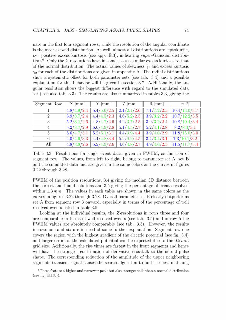
CHAPTER 3. JASS - SIMULATING AGATA PULSE SHAPES 74
nate in the first four segment rows, while the resolution of the angular coordinateis the most skewed distribution. As well, almost all distributions are leptokurtic,i.e. positive excess kurtosis (see app. E.3), indicating super -Gaussian distribu-tions6. Only the Z resolutions have in some cases a similar excess kurtosis to thatof the normal distribution. The actual values of skewness γ1 and excess kurtosisγ2 for each of the distributions are given in appendix A. The radial distributionsshow a systematic offset for both parameter sets (see tab. 3.4) and a possibleexplanation for this behavior will be given in section 3.7. Additionally, the an-gular resolution shows the biggest difference with regard to the simulated dataset ( see also tab. 3.3). The results are also summarized in tables 3.3, giving the
Segment Row X [mm] Y [mm] Z [mm] R [mm] ϕ []
1 4.8/4.9/2.4 5.4/5.0/2.5 2.1/2.1/2.6 7.1/7.2/2.5 10.4/13.0/3.72 3.9/3.7/2.4 4.4/4.5/2.3 4.6/5.2/2.5 3.9/3.2/2.2 10.7/12.2/3.53 5.2/3.1/2.6 4.8/4.7/2.6 4.2/3.7/2.5 3.9/3.2/2.4 10.8/10.4/3.44 5.2/3.7/2.9 6.0/4.9/2.8 5.1/4.5/2.7 5.2/4.1/2.8 8.2/8.3/3.15 5.6/4.7/3.1 5.2/5.1/3.1 4.4/3.9/4.4 3.9/4.0/2.9 11.8/15.0/3.06 4.0/4.6/3.3 4.4/4.8/3.4 5.2/9.2/4.5 3.4/3.4/3.1 7.3/10.1/3.2
All 4.8/3.8/2.6 5.2/4.9/2.6 4.6/4.8/2.7 4.9/4.6/2.5 11.5/11.7/3.4
Table 3.3: Resolutions for single event data, given in FWHM, as function ofsegment row. The values, from left to right, belong to parameter set A, set Band the simulated data and are given in the same colors as the curves in figures3.22 through 3.28
FWHM of the position resolutions, 3.4 giving the median 3D distance betweenthe correct and found solutions and 3.5 giving the percentage of events resolvedwithin ±3mm. The values in each table are shown in the same colors as thecurves in figures 3.22 through 3.28. Overall parameter set B clearly outperformsset A from segment row 3 onward, especially in terms of the percentage of wellresolved events listed in table 3.5.
Looking at the individual results, the Z-resolutions in rows three and fourare comparable in terms of well resolved events (see tab. 3.5) and in row 5 theFWHM values are absolutely comparable (see tab. 3.3). However, the resultsin rows one and six are in need of some further explanation. Segment row onecovers the region with the highest gradient of the electric potential (see fig. 3.4)and larger errors of the calculated potential can be expected due to the 0.5mmgrid size. Additionally, the rise times are fastest in the front segments and hencewill have the strongest contribution of derivative crosstalk to the actual pulseshape. The corresponding reduction of the amplitude of the upper neighboringsegments transient signal causes the search algorithm to find the best matching
6These feature a higher and narrower peak but also stronger tails than a normal distribution(see fig. E.1(b)).

CHAPTER 3. JASS - SIMULATING AGATA PULSE SHAPES 75
Feature Row 1 Row 2 Row 3 Row 4
Median 3D [mm] 3.9/4.5/1.5 3.4/3.5/1.5 3.3/2.7/1.6 3.5/3.0/1.9Mean Radial Offset [mm] 0.5/−1.7/0.3 1.2/0.2/0.1 1.6/0.5/0.0 1.5/0.2/0.1
Row 5 Row 6 AllMedian 3D [mm] 3.8/3.5/2.2 5.7/5.1/4.3 3.6/3.5/1.7
Mean Radial Offset [mm] 1.0/−0.3/0.1 0.7/−0.7/0.4 1.1/−0.5/0.1
Table 3.4: The median 3D distance between the correct position and the foundsolution and radial offset for each segment row. The values, from left to right,belong to parameter set A, set B and the simulated data and are given in thesame colors as the curves in figures 3.22 through 3.28
Segment Row X [mm] Y [mm] Z [mm] R [mm]
1 84.6/72.9/97.4 74.6/71.2/98.1 91.6/91.5/97.7 76.7/63.9/97.22 82.5/81.6/97.5 82.4/81.5/98.0 94.2/91.7/97.9 92.9/97.8/99.03 84.4/91.5/97.5 80.1/89.2/97.9 97.1/97.9/97.7 86.3/96.9/99.34 85.8/89.8/96.6 80.1/87.7/93.7 94.0/94.4/95.3 82.8/94.5/98.15 84.0/84.8/96.0 80.4/83.8/95.7 82.9/84.6/94.5 86.0/91.1/97.86 84.2/83.8/95.1 84.3/82.8/94.6 49.8/55.0/92.8 90.7/89.2/97.8
All 84.5/82.6/97.1 78.4/80.9/97.1 92.2/92.4/96.8 82.9/83.6/98.1
Table 3.5: Percentage of events resolved within ±3mm as function of segmentrow. The values, from left to right, belong to parameter set A, set B and thesimulated data and are given in the same colors as the curves in figures 3.22through 3.28

CHAPTER 3. JASS - SIMULATING AGATA PULSE SHAPES 76
0 20 40 60 80 100 120−0.2
0
0.2
0.4
0.6
0.8
1
1.2
Sample Index
Nor
mal
ized
Cha
rge
(a) Net charge signal in segment F1
0 20 40 60 80 100 120−0.12
−0.1
−0.08
−0.06
−0.04
−0.02
0
0.02
0.04
0.06
Sample Index
Nor
mal
ized
Cha
rge
(b) Transient signal in segment F2.
0 20 40 60 80 100 120−0.2
−0.15
−0.1
−0.05
0
0.05
Sample Index
Nor
mal
ized
Cha
rge
(c) Transient signal in segment A1.
0 20 40 60 80 100 120−0.05
−0.04
−0.03
−0.02
−0.01
0
0.01
0.02
Sample Index
Nor
mal
ized
Cha
rge
(d) Transient signal in segment E1.
Figure 3.29: Comparison between scanned (red, +) and simulated signals for aninteraction in segment F1. As can be seen in (b) the simulated transient signalsin segment F2 still have a too large amplitude although their locations are atthe absolute front of the detector. The nominal location of the scan point is(x,y,z)=(16.3,-11.7,3.1), the location found with parameter set A (blue, solid) is(11.75,-11,1) and (13.75,-11,2) with parameter set B (green, dashed).

CHAPTER 3. JASS - SIMULATING AGATA PULSE SHAPES 77
signals to the scanning signals at z = 3.3mm at the utmost front of the basisset at Z = 1mm (see figs. 3.22(c) and 3.29). Figure 3.29(b) clearly shows theamplitude of the simulated transient signals in the upper neighboring segmentis still to large at these locations. Excluding these events changes the FWHMof the Z resolution to 3.6mm for parameter set A and 3.2mm for parameterset B. The median 3D distance decreases to 2.5mm and 2.6mm respectively, afact that is easily explained since at a depth of z = 14.8mm, which is insidethe physical boundaries of the second segment row (see fig. 3.5), the number ofbasis points with a well matching transient signal, which will inevitably have alarge amplitude, in the upper neighboring segment is rather low. Concerning theresult in row six it should be noted that, due to the crystal being completelycoaxial in this area, only the transient signal in the lower neighboring segmentcarries information on the Z-position of the γ-ray interaction. Conversely, thenet charge signal in the first five segment rows also contains information on the Zposition due to the tapering of the crystal. The results for parameter sets A and
0 50 100 150 200 250−0.05
0
0.05
0.1
0.15
0.2
Sample Index
No
rma
lize
d C
ha
rge
(a) Transient signal in segment B6.
0 50 100 150 200 250−0.04
−0.02
0
0.02
0.04
0.06
0.08
0.1
0.12
0.14
0.16
Sample Index
No
rma
lize
d C
ha
rge
(b) Transient signal in segment A5.
Figure 3.30: Comparison of three scan signals in segment A6 with the samenominal position close to the boundary with segment B6. The great scatterin transient amplitude, especially in (b), is obvious and related to the limitedprecision of the scanning setup.
B suffer from the limited precision of the scanning setup and subsequent largevariation in signal shape, evident in figure 3.30. The amplitude of the transientsignal in segment A5 varies by more than a factor of two (see fig. 3.30(b)) causingthe found positions to be systematically shifted to lower Z values (black curve),close to the nominal position (green curve) or shifted to larger Z values (bluecurve). Judging from the achieved resolutions the nominal green curve seemsto be the exception rather than the rule. Parameter set B resolves the radialcoordinate far better than set A with more than 90% of well resolved events (seetab. 3.5) and a better FWHM for most segment rows (see tab. 3.3). This hintsat a better match with the experimental rise times for set B (see sec. 3.7). The
CHAPTER 3. JASS - SIMULATING AGATA PULSE SHAPES 78
angular resolution, by contrast, shows the biggest deviations from the optimalvalues and also between the two parameter sets. The latter is not that surprisingsince the parameter sets do not only lead to different signal rise times at a givenposition, but also to different amplitudes of the transient signals (see fig. 3.31).Additionally, the angular resolution suffers the most from the lack of a derivativecrosstalk correction since it is solely determined by the transient signals in theleft and right neighboring segments. Rather surprisingly the angular resolutionfor set A is best in row six, while row four produces the best results for set B. Thelast point to mention concerns the median 3D distance, its limit increases fromthe front to the back of the crystal, in line with the reduced position sensitivitydue to larger segments and the increasing position uncertainties of the setup.This feature is not reproduced by either parameter set although the last segmentrow also has the largest median distance for both parameter sets. However, thedeviation form the limit is smaller than in the front segment rows suggesting thatthe current scanning setup is not sensitive enough to detect this characteristic.Overall the results are best in the middle of the crystal, rows three and four, withparameter set B performing within the limits set for PSA (see tab. 4.1).
3.7 Discussion
The two main issues to discuss are the precision of the simulated data on oneside and the performance of the scanning system on the other side. Regardingthe latter, a new data acquisition system for the scanning setup in Liverpoolis being installed which will considerably increase the quality of the data. Thesegment signals will all be time aligned, as with the AGATA DAQ (see sec. 2.2),allowing for a determination of the derivative crosstalk component. This is veryimportant for a precise comparison with the simulated data set. Additionally, theposition uncertainties of the setup could be significantly reduced by employingthe scanning method from (Crespi et al., 2008). The basic idea of the Pulse
Shape Comparison Scan (PSCS) is to use a collimated source and illuminate thecrystal from two perpendicular position (see fig. 3.32), (a) and (b). The pulseshapes from both data sets are then compared by calculating all χ2 values betweenone pulse shape from position (a) and the other pulse shape from position (b).Naturally, the only time a good agreement between both signals can be foundis if they belong to the same location within the crystal (see next paragraph).According to the authors a position uncertainty of σx,y,z < 1mm can be achievedby selecting a stringent χ2 threshold and a full detector characterization shouldtake only one week.
Concerning the simulation there are a few things to mention. First of allduring the course of this work it was found that, contrary to previous beliefs,the radial distribution of impurities, e.g. either flat or with linear gradient, hasno significant influence on the pulse shape given that both distributions have the

CHAPTER 3. JASS - SIMULATING AGATA PULSE SHAPES 79
0 20 40 60 80 100 120−0.2
0
0.2
0.4
0.6
0.8
1
1.2
Sample Index
Nor
mal
ized
Cha
rge
(a) Net charge signal in segment A4
0 20 40 60 80 100 120−0.12
−0.1
−0.08
−0.06
−0.04
−0.02
0
0.02
0.04
Sample Index
Nor
mal
ized
Cha
rge
(b) Transient signal in segment A5.
0 20 40 60 80 100 120−0.06
−0.04
−0.02
0
0.02
0.04
0.06
Sample Index
Nor
mal
ized
Cha
rge
(c) Transient signal in segment A3.
0 20 40 60 80 100 120−0.03
−0.02
−0.01
0
0.01
0.02
0.03
Sample Index
Nor
mal
ized
Cha
rge
(d) Transient signal in segment B4.
0 20 40 60 80 100 120−0.14
−0.12
−0.1
−0.08
−0.06
−0.04
−0.02
0
0.02
0.04
Sample Index
Nor
mal
ized
Cha
rge
(e) Transient signal in segment F4.
Figure 3.31: Comparison between scanned (red, +) and simulated signals foran interaction in segment A4. The nominal location of the scan point is(x,y,z)=(28.3,-13.6,47.7), the location found with parameter set A (blue, solid) is(29.75,-11,52) and (28.75,-12,49) with parameter set B (green, dashed).
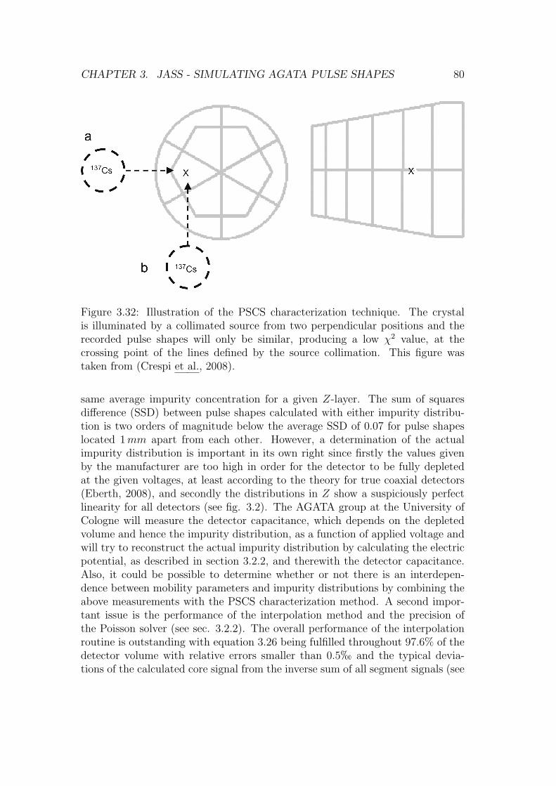
CHAPTER 3. JASS - SIMULATING AGATA PULSE SHAPES 80
Figure 3.32: Illustration of the PSCS characterization technique. The crystalis illuminated by a collimated source from two perpendicular positions and therecorded pulse shapes will only be similar, producing a low χ2 value, at thecrossing point of the lines defined by the source collimation. This figure wastaken from (Crespi et al., 2008).
same average impurity concentration for a given Z-layer. The sum of squaresdifference (SSD) between pulse shapes calculated with either impurity distribu-tion is two orders of magnitude below the average SSD of 0.07 for pulse shapeslocated 1mm apart from each other. However, a determination of the actualimpurity distribution is important in its own right since firstly the values givenby the manufacturer are too high in order for the detector to be fully depletedat the given voltages, at least according to the theory for true coaxial detectors(Eberth, 2008), and secondly the distributions in Z show a suspiciously perfectlinearity for all detectors (see fig. 3.2). The AGATA group at the University ofCologne will measure the detector capacitance, which depends on the depletedvolume and hence the impurity distribution, as a function of applied voltage andwill try to reconstruct the actual impurity distribution by calculating the electricpotential, as described in section 3.2.2, and therewith the detector capacitance.Also, it could be possible to determine whether or not there is an interdepen-dence between mobility parameters and impurity distributions by combining theabove measurements with the PSCS characterization method. A second impor-tant issue is the performance of the interpolation method and the precision ofthe Poisson solver (see sec. 3.2.2). The overall performance of the interpolationroutine is outstanding with equation 3.26 being fulfilled throughout 97.6% of thedetector volume with relative errors smaller than 0.5h and the typical devia-tions of the calculated core signal from the inverse sum of all segment signals (see

CHAPTER 3. JASS - SIMULATING AGATA PULSE SHAPES 81
eqn. 3.27) are of the order of 10−8. Figure 3.33 shows one of the worst cases
0 20 40 60 80 100 120 140 160 180 2000
0.5
1
1.5
Time [ns]
No
rma
lize
d C
ha
rge
0 20 40 60 80 100 120 140 160 180 200−0.1
−0.05
0
0.05
0.1Residual
Time [ns]No
rma
lize
d C
ha
rge
Figure 3.33: Comparison between the inverse sum of the segment signals and thecore signal for the worst case. The upper panel shows the sum signal in blue andthe core signal in a red dash-dotted line. The lower panel shows the residual,which is only significant at the end where the trajectory of the holes gets closeto the segment boundary.
with the sum of segment signals significantly overshooting toward the end. Inthis exemplary case the trajectory ends at the lower right edge of the hit segmentelectrode. As the interpolation routine smooths the discontinuous drop from unitcharge to zero at the segment boundaries (see fig. 3.14), the weighing potentialsof the three neighboring segments are assigned too large values causing the sumof all weighting potentials (see 3.26) to be larger than unity and in turn the seg-ment signal to overshoot the core signal. The first 0.5mm after the front sideelectrodes prove to be rather difficult as well, even more so in the center regionwith the six pointed tips of the electrodes. Since the precision of the calculatedelectric potential in the area between the core contact and the front side elec-trodes is also worse than in the rest of the detector an increase in resolutionwould improve both precisions. The only possibility with the current approachis to selectively reduce the step size in Z direction to 0.25mm and still keep thememory requirements down to manageable amounts. However, this would notimprove the interpolation performance near the remaining segment boundaries.The most demanding possibility would be to use an adaptive multigrid solver (seee.g. (Trottenberg et al., 2000),pages 356 ff.), which uses cubes of adaptive sizeto discretize the problem to solve with the size being chosen according to the de-

CHAPTER 3. JASS - SIMULATING AGATA PULSE SHAPES 82
sired precision and adapted to the local gradients. Concerning a good agreementbetween simulated and experimental signals, though, the charge carrier mobilityparameters and the derivative crosstalk are the most important components. Inabsence of the latter, no final conclusion on the examined parameter sets can bedrawn, although neither seems to achieve a very good match with the scanneddata set throughout the detector. Yet, the systematic deviations of the radial
5 10 15 20 25 30 35 40−2
−1
0
1
2
3
4
5
Radial Position [mm]
Me
an
Ra
dia
l O
ffse
t [m
m]
(a) Mean radial offset in segment row 3.
5 10 15 20 25 30 35 40−2
−1
0
1
2
3
4
5
Radial Position [mm]
Me
an
Ra
dia
l O
ffse
t [m
m]
(b) Mean radial offset in segment row 4.
5 10 15 20 25 30 35 40−2
−1
0
1
2
3
4
5
Radial Position [mm]
Me
an
Ra
dia
l O
ffse
t [m
m]
(c) Mean radial offset in segment row 5.
5 10 15 20 25 30 35 40−2
−1
0
1
2
3
4
5
Radial Position [mm]
Me
an
Ra
dia
l O
ffse
t [m
m]
(d) Mean radial offset in segment row 6.
Figure 3.34: This figure shows the mean radial offsets between the found andcorrect radial position in segment rows 3 through 6 as a function of the correctradial position. The individual values were calculated within intervals of 5 mm,indicated by the horizontal bars with the lines being drawn to guide the eye.The red dashed line corresponds to parameter set B, and the solid blue line toparameter set A. The average absolute displacement with the simulated data setis smaller than 0.4mm.
coordinate (see fig. 3.34), predominantly influenced by the net charge signal andthus not influenced by derivative crosstalk, allow for some conclusions regard-ing the relation of the true drift velocities and signal rise times to those of the

CHAPTER 3. JASS - SIMULATING AGATA PULSE SHAPES 83
used parameter sets (see tabs. B.1 and B.2). However, this is only true fromsegment row three onwards as there is a considerable vertical drift component inthe first two segment rows, preventing a clear relation between the drift time andthe radial position. Therefore, figure 3.34 shows the mean deviation between thefound and correct radial positions as function of the correct radial position inbins of 5mm width only for segment rows three through six. As can be seen, pa-rameter set B reproduces the drift velocities rather accurately in rows three andfour with the offsets being of the order of 0.5mm. Conversely, the radial offsetsof parameter set A are always around 1mm indicating too slow drift velocities.The deviations grow larger in segment rows five and six, yet both follow the samesystematic.
This is likely related to the influence of the passivated layer at the back ofthe crystal. This layer can be up to 7mm thick and reduces the electric fieldstrength (Eberth & Simpson, 2008). Taking the significant position uncertaintiesof the scanning setup into account an optimization of the mobility parametersand subsequent optimization of the radial offsets, is only meaningful when usingthe PSCS method, described above.

Chapter 4
Pulse Shape Analysis
Pulse shape analysis (PSA) is the single most important issue in the AGATADAQ as it is impossible to reduce the data to manageable amounts without aworking PSA (see sec. 2.2). It’s goal is to reconstruct in real time and with highprecision the position, energy and time of each individual γ-interaction based onthe recorded pulse shapes. Previous attempts on data from the MARS detectorwere successful in achieving a good position resolution of 2−8mm (FWHM), yetonly on a timescale of around 1 s (Kroll & Bazzacco, 2006), too long for the realtime DAQ of AGATA. In the following section the requirements of the AGATAPSA, the basic approach taken and the challenges involved will be discussed.Feedforward neural networks, used to determine the event time, will be introducedin section 4.2. The interaction positions will be reconstructed by a particle swarmoptimization algorithm, delineated in section 4.3.
4.1 Introduction to AGATA PSA
As was already mentioned the aim of PSA is to determine the number of inter-actions in a segment or crystal and to reconstruct the positions, time and thedeposited energy of each individual γ-ray interaction by analyzing the recordedexperimental traces. The real-time frame work of the AGATA DAQ and therequirements of the tracking algorithms demand stringent performance require-ments for the PSA algorithm summarized in the following table.
Parameter Requirement
Position Resolution ≤ 5mm (FWHM)Energy Resolution ∼ 3 keVTime Resolution < 10nsComputing Time ∼ 1ms/CPU
Table 4.1: The performance requirements for the PSA algorithm.
84

CHAPTER 4. PULSE SHAPE ANALYSIS 85
The PSA utilizes the strong dependence of each single pulse shape on theinteraction location. Yet the complete information on the interaction location isnot stored in a single pulse shape but in the combination of pulse shapes (see fig.4.1). The transient traces in the neighboring segments to the left and right of thehit segment are most sensitive to the angular position of the interaction while thesegments above and below record the most information of all crystal segments onthe distance from the front face. The amplitudes of these transient signals dependin a highly non-linear fashion on the distance of the charge carriers trajectoryto the neighboring segments. The radial coordinate has the biggest influence onthe net charge signal and to a significant extent on the core signal. If one of thecharge carriers is collected a discontinuous drop in the current occurs, recorded asa kink in the charge signal (see fig. 3.11). Its position in time gives informationon the electron drift time ted and hence the radial position of the interaction.However, the attainable position resolution is not only limited by electronic noise
0 100 200 300 400 500 6000
0.1
0.2
0.3
0.4
0.5
0.6
0.7
0.8
0.9
1
Time [ns]
No
rma
lize
d C
ha
rge
Hit Segment
0 100 200 300 400 500 600−1
−0.9
−0.8
−0.7
−0.6
−0.5
−0.4
−0.3
−0.2
−0.1
0Core Signal
Time [ns]
No
rma
lize
d C
ha
rge
0 100 200 300 400 500 600−0.3
−0.25
−0.2
−0.15
−0.1
−0.05
0
0.05Left Neighbour
Time [ns]
No
rma
lize
d C
ha
rge
0 100 200 300 400 500 600−0.5
−0.4
−0.3
−0.2
−0.1
0
0.1
0.2Right Neighbour
Time [ns]
No
rmla
ize
d C
ha
rge
R=19 mm, φ=150°
R=19 mm, φ=210°
R=10 mm, φ=180°
R=30 mm, φ=180°
Figure 4.1: The dependence of the pulse shapes on the interaction location. Thered and blue shapes differ only in their angular position yet the core signalsare almost identical and the net charge signals in the hit segments differ onlymarginally. The transient signals in the left and right neighbors, shown in thelower panel, by contrast, are easily distinguished. The opposite is observed forthe black and green shapes representing two different radial positions.
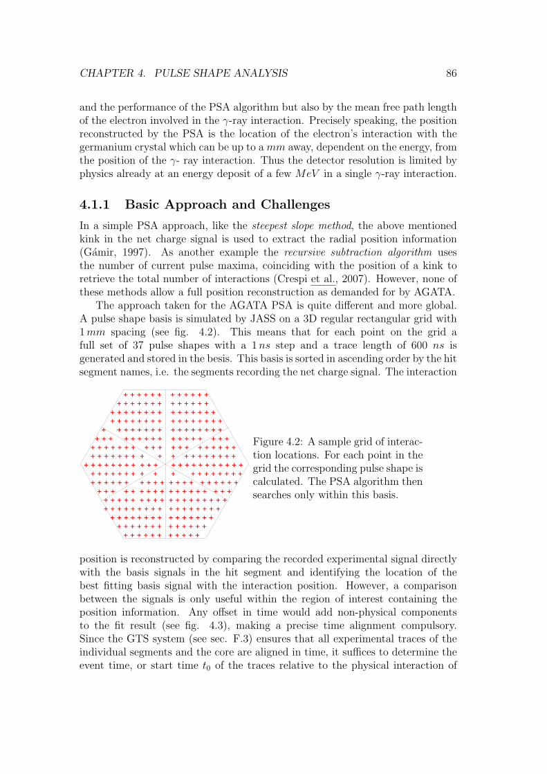
CHAPTER 4. PULSE SHAPE ANALYSIS 86
and the performance of the PSA algorithm but also by the mean free path lengthof the electron involved in the γ-ray interaction. Precisely speaking, the positionreconstructed by the PSA is the location of the electron’s interaction with thegermanium crystal which can be up to a mm away, dependent on the energy, fromthe position of the γ- ray interaction. Thus the detector resolution is limited byphysics already at an energy deposit of a few MeV in a single γ-ray interaction.
4.1.1 Basic Approach and Challenges
In a simple PSA approach, like the steepest slope method, the above mentionedkink in the net charge signal is used to extract the radial position information(Gamir, 1997). As another example the recursive subtraction algorithm usesthe number of current pulse maxima, coinciding with the position of a kink toretrieve the total number of interactions (Crespi et al., 2007). However, none ofthese methods allow a full position reconstruction as demanded for by AGATA.
The approach taken for the AGATA PSA is quite different and more global.A pulse shape basis is simulated by JASS on a 3D regular rectangular grid with1mm spacing (see fig. 4.2). This means that for each point on the grid afull set of 37 pulse shapes with a 1ns step and a trace length of 600 ns isgenerated and stored in the besis. This basis is sorted in ascending order by the hitsegment names, i.e. the segments recording the net charge signal. The interaction
Figure 4.2: A sample grid of interac-tion locations. For each point in thegrid the corresponding pulse shape iscalculated. The PSA algorithm thensearches only within this basis.
position is reconstructed by comparing the recorded experimental signal directlywith the basis signals in the hit segment and identifying the location of thebest fitting basis signal with the interaction position. However, a comparisonbetween the signals is only useful within the region of interest containing theposition information. Any offset in time would add non-physical componentsto the fit result (see fig. 4.3), making a precise time alignment compulsory.Since the GTS system (see sec. F.3) ensures that all experimental traces of theindividual segments and the core are aligned in time, it suffices to determine theevent time, or start time t0 of the traces relative to the physical interaction of

CHAPTER 4. PULSE SHAPE ANALYSIS 87
the γ-ray in the detector material, for just one signal. The core signal has theleast dependence on location (see fig. 4.1) and interaction multiplicity and thusis best suited to determine t0 independent of the position reconstruction. Theindependent determination of t0 removes one parameter from the PSA searchspace and simplifies the remaining task considerably. Additionally, the reducedvariability of the core signal facilitates the use of neural networks to determinet0 (see sec. 5.1).
The description so far concentrated on single interactions only. While there isno principal difficulty preventing the chosen approach to be used for events withmultiple interactions in the crystal, the task becomes a lot more challenging. Theparticular challenge lies in the binomial growth of the search space with inter-action multiplicity. Each segment contains between 5000 and 15000 grid pointsto be searched for agreement with the experimental signal. An extensive search,i.e. comparing the pulse shapes of each single grid point with the experimentalsignal, of the segments basis takes between 40 and 200ms in the case of singleinteractions, just about in the performance requirements (see tab. 4.1). For the
Hit Number of InteractionsSegments 1 2 3 4 5
15.00E+003- 1.25E+007- 1.04E+010- 2.17E+012- 9.02E+013-1.50E+004 1.12E+008 2.81E+011 1.76E+014 2.20E+016
2 X2.50E+007- 6.25E+010- 1.56E+014- 1.30E+017-2.25E+008 1.69E+012 1.27E+016 3.16E+019
3 X X1.25E+011- 3.12E+014- 7.81E+017-3.38E+012 2.53E+016 1.90E+020
4 X X X6.25E+014- 1.56E+018-5.06E+016 3.80E+020
5 X X X X3.13E+018-7.59E+020
Table 4.2: Number of possible basis point combinations depending on the eventtype. The lower limit is for segments with 5000 basis points and the upper limit isfor 15000 basis points. Impossible combinations, e.g. 1 interaction in 2 segments,are marked by an X and in case there is more than one possibility for a given eventtype, e.g. four interactions in two segments can either be 3:1 or 2:2 distributedamong the segments, the larger number is quoted in the table.
case of two interactions in the same segment the pulse shapes for each interac-tion have to be added, scaled linearly with energy, and the number of possiblecombinations of grid points grows to 1.25 · 107 − 1.12 · 108, quickly ruling outthe extensive search. In addition the energy of each interaction adds in totalone more free parameter1. Table 4.2 summarizes the size of the search space for
1The total energy deposit in a segment is given by the front end electronics (see sec. F.3),
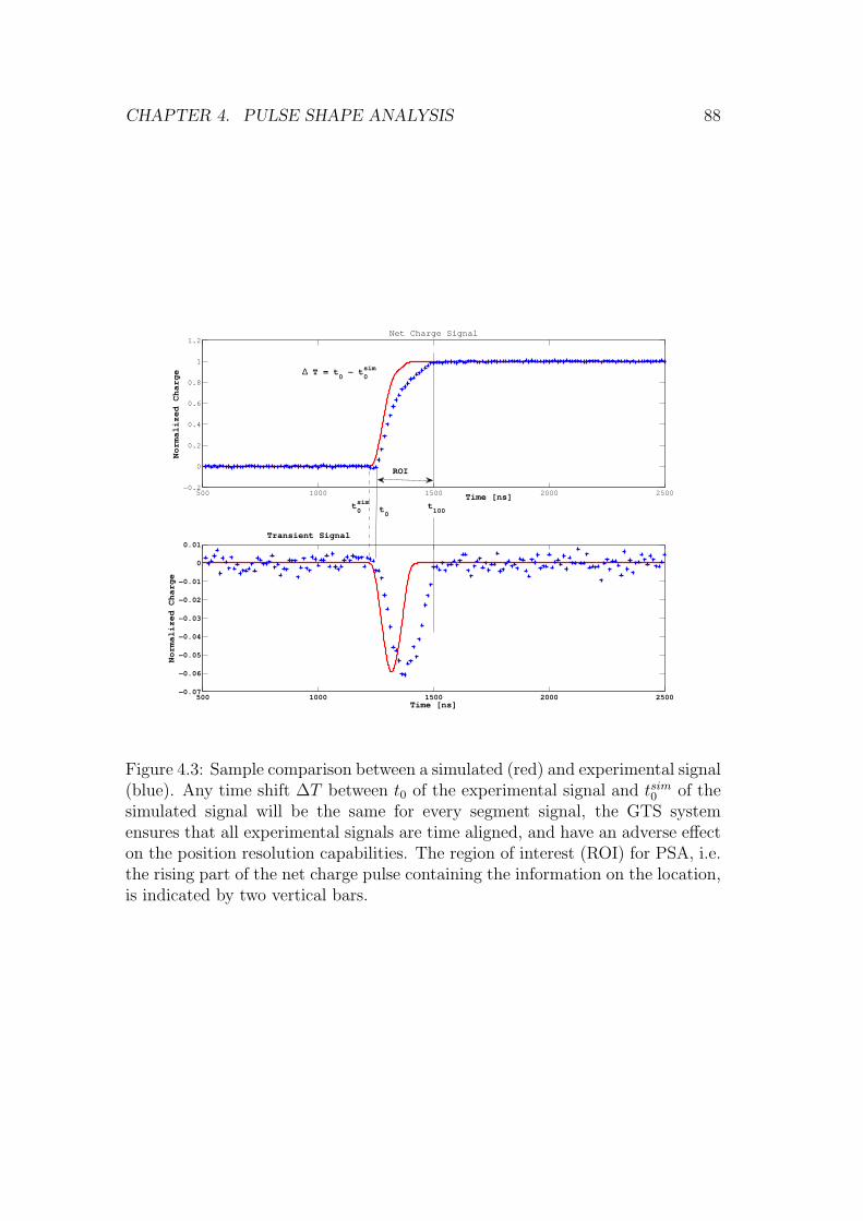
CHAPTER 4. PULSE SHAPE ANALYSIS 88
500 1000 1500 2000 2500−0.07
−0.06
−0.05
−0.04
−0.03
−0.02
−0.01
0
0.01Transient Signal
Time [ns]
No
rma
lize
d C
ha
rge
500 1000 1500 2000 2500−0.2
0
0.2
0.4
0.6
0.8
1
1.2
Time [ns]
No
rma
lize
d C
ha
rge
Net Charge Signal
t100
ROI
t0
t0sim
∆ T = t0 − t
0sim
Figure 4.3: Sample comparison between a simulated (red) and experimental signal(blue). Any time shift ∆T between t0 of the experimental signal and tsim0 of thesimulated signal will be the same for every segment signal, the GTS systemensures that all experimental signals are time aligned, and have an adverse effecton the position resolution capabilities. The region of interest (ROI) for PSA, i.e.the rising part of the net charge pulse containing the information on the location,is indicated by two vertical bars.

CHAPTER 4. PULSE SHAPE ANALYSIS 89
various multiple interaction events. These numbers exemplify the need for anintelligent search algorithm, like Particle Swarm Optimization (see sec. 4.3), forthe position reconstruction. Other approaches like the matrix method (Olariuet al., 2006), which uses a non-negative least squares algorithm to assign energydeposits for all grid points simultaneously followed by a calculation of the ener-getic barycenters, have so far not been able to meet the requirements in terms ofspeed for these multiple
4.2 Feedforward Neural Networks
In AGATA PSA a neural network will be used to determine the event time t0, i.e.the start time of the experimental signal (see fig. 4.3). The much more compli-cated task of position reconstruction will be performed by the particle swarm op-timization (see sec. 4.3). The different types of artificial neural networks (ANN)that exist are almost as diverse as their field of use. Starting out from the simpleperceptron developed by (Rosenblatt, 1958) and application to the XOR problem(Minsky & Papert, 1969) newer forms like Radial Basis Function networks (Bors,2000) have been developed. Spiking Neural Networks (Bothe, 2003) are the lat-est development and claim to be one step closer to the biological original of abrain. Possible applications range from simple function approximations (Hornik,1991) over artificial intelligence in computer games to help in controlling fighterjets (NASA, 2006). Feedforward neural networks (FNN) have been shown to bevery efficient for problems of pattern recognition (Bishop, 1996), similar to theintended use of a neural network for AGATA. Therefore the following descriptionwill cover only FNN and introduce the topology and training methods for thesetypes of ANN.
4.2.1 Topology of a network
The topology of a FNN is relatively simple yet still features massively parallelcomputations. The basic computational unit is a so called neuron, in reference tothe neurons found in a brain. A FNN, however, is only an oversimplified versionof a brain in the still limited understanding of a brains inner working. Basicallyonly the idea of having small but independent computational units, the neurons,which are strongly interconnected, is used to form a working computer algorithm.Each neuron in the FNN has an internal state dependent on the received inputsand an activation function, which determines the neurons output. In order toassemble a FNN these neurons are arranged in separate layers. The input stageis counted as the networks first layer passing on its values to the neurons in thenext layer. If this layer is already the final layer it is called the output layer giving
so for two interactions only the ratio of energy deposits for the two interactions has to bedetermined.

CHAPTER 4. PULSE SHAPE ANALYSIS 90
b1(4)b1(2) b1(3)
f 11 f 1
2 f 13 f 1
4
∑ ∑
w1(4, 4)w1(1, 1)
∑∑
b2(2)
w2(2, 4)
f 21 f 2
2
a2(1) a2(2)
b2(1)
w2(1, 1)
a1(1) a1(2) a1(3) a1(4)
∑ ∑
I1 I2 I3 I4
b1(1)
Figure 4.4: Topology of a two-layer feedforward network. The first layer is theinput stage passing the values Ii after weighting with the weights wk(i, j) tothe neurons in the hidden layer. Each neuron then adds its own bias b1(i) tothe just calculated weighted sum of the inputs. The neurons output a1(i) isthen computed by applying the activation function f 1 and sent to all connectedneurons, but only in forward direction (from top to bottom in the picture). Thenetworks outputs, in this example, are a2(1) and a2(2).
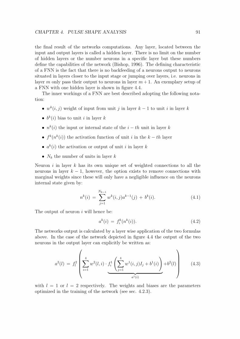
CHAPTER 4. PULSE SHAPE ANALYSIS 91
the final result of the networks computations. Any layer, located between theinput and output layers is called a hidden layer. There is no limit on the numberof hidden layers or the number neurons in a specific layer but these numbersdefine the capabilities of the network (Bishop, 1996). The defining characteristicof a FNN is the fact that there is no backfeeding of a neurons output to neuronssituated in layers closer to the input stage or jumping over layers, i.e. neurons inlayer m only pass their output to neurons in layer m+ 1. An exemplary setup ofa FNN with one hidden layer is shown in figure 4.4.
The inner workings of a FNN are best described adopting the following nota-tion:
• wk(i, j) weight of input from unit j in layer k − 1 to unit i in layer k
• bk(i) bias to unit i in layer k
• nk(i) the input or internal state of the i− th unit in layer k
• fk(nk(i)) the activation function of unit i in the k − th layer
• ak(i) the activation or output of unit i in layer k
• Nk the number of units in layer k
Neuron i in layer k has its own unique set of weighted connections to all theneurons in layer k − 1, however, the option exists to remove connections withmarginal weights since these will only have a negligible influence on the neuronsinternal state given by:
nk(i) =
Nk−1∑
j=1
wk(i, j)ak−1(j) + bk(i). (4.1)
The output of neuron i will hence be:
ak(i) = fki (nk(i)). (4.2)
The networks output is calculated by a layer wise application of the two formulasabove. In the case of the network depicted in figure 4.4 the output of the twoneurons in the output layer can explicitly be written as:
a2(l) = f 2l
4∑
i=1
w2(l, i) · f 1i
(4∑
j=1
w1(i, j)Ij + b1(i)
)
︸ ︷︷ ︸
a1(i)
+b2(l)
(4.3)
with l = 1 or l = 2 respectively. The weights and biases are the parametersoptimized in the training of the network (see sec. 4.2.3).

CHAPTER 4. PULSE SHAPE ANALYSIS 92
4.2.2 Activation Functions
The concept of FNN was introduced by (Rosenblatt, 1958)2 using the Heavisidestep function for activating the neurons and featuring no hidden layer. This notonly limited the output to binary values but also the general applicability of sucha network, e.g. function approximation demands a linear activation function inthe output layer ((Hornik, 1991)). The three different activation functions, whichare nowadays typically used are the
• Linear function: ak(i) = nk(i)
• Sigmoid function: ak(i) =(1 + exp (−nk(i))
)−1
• Hyperbolic tangent: ak(i) = tanh (nk(i)).
These differ in their range of application. The linear function is the only onewhich output can access the complete R. Hence the activation function of theoutput layer for network used in function approximation has to be the linearfunction. The active region, the input interval for which the functions output isnot saturated, of the sigmoid function is larger than for the tanh function (seefig.4.5), which can be advantageous if the inputs are spread over a larger inter-val. Also the limitation to outputs within [0, 1] makes it the natural choice forapproximating probabilities or possibly for the interpolation of weighting poten-tials (see sec. 3.3). Yet the tanh function is the most common choice, especiallyfor neurons in a hidden layer. First of all the rather small size of its active re-gion, from −1 to 1 allows for sharp decision boundaries, advantageous for patternrecognition. Secondly it allows a neuron to not only exert an excitatory but alsoan inhibitory influence on other neurons whilst its output range of [−1, 1] is stilllimited in contrast to the linear function. Lastly is should be mentioned that therole of the bias is to move the zero-crossing point of the activation functions awayfrom the origin.
4.2.3 Training and Validation
No mathematical prescription exists to calculate the weights and biases of anetwork solely based on its intended use other than in the most simple cases likethe XOR-problem. Instead a network has to adapt its parameters in a learningprocess. There are two main, yet distinctively different learning paradigms forneural networks. In unsupervised learning only a set of input data I is given butthe target output O of the network is not. The goal of the learning process is tooptimize a given cost function C(I, O) which can take on quite complicated forms.Typical tasks treated with unsupervised learning are clustering and estimationof statistical distributions and can generally be classified as estimation problems.
2The original name used in the paper was perceptron.

CHAPTER 4. PULSE SHAPE ANALYSIS 93
−8 −6 −4 −2 0 2 4 6 8−2
−1.5
−1
−0.5
0
0.5
1
1.5
2
x
f(x)
LinearSigmoidTanh
Figure 4.5: The three different activation functions typically used for FNN. Onlythe linear function can access the complete R and has an infinite active region,making it ideal to use for function approximation problems. The sigmoid functionhas a considerably larger active region, e.g. area of non-saturated output, thanthe tanh function and the smallest slope around the origin.
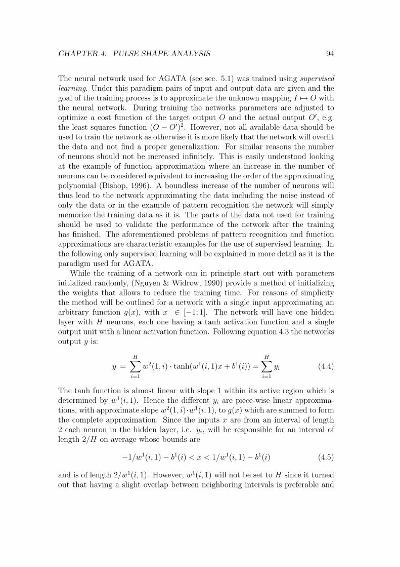
CHAPTER 4. PULSE SHAPE ANALYSIS 94
The neural network used for AGATA (see sec. 5.1) was trained using supervised
learning. Under this paradigm pairs of input and output data are given and thegoal of the training process is to approximate the unknown mapping I 7→ O withthe neural network. During training the networks parameters are adjusted tooptimize a cost function of the target output O and the actual output O′, e.g.the least squares function (O − O′)2. However, not all available data should beused to train the network as otherwise it is more likely that the network will overfitthe data and not find a proper generalization. For similar reasons the numberof neurons should not be increased infinitely. This is easily understood lookingat the example of function approximation where an increase in the number ofneurons can be considered equivalent to increasing the order of the approximatingpolynomial (Bishop, 1996). A boundless increase of the number of neurons willthus lead to the network approximating the data including the noise instead ofonly the data or in the example of pattern recognition the network will simplymemorize the training data as it is. The parts of the data not used for trainingshould be used to validate the performance of the network after the traininghas finished. The aforementioned problems of pattern recognition and functionapproximations are characteristic examples for the use of supervised learning. Inthe following only supervised learning will be explained in more detail as it is theparadigm used for AGATA.
While the training of a network can in principle start out with parametersinitialized randomly, (Nguyen & Widrow, 1990) provide a method of initializingthe weights that allows to reduce the training time. For reasons of simplicitythe method will be outlined for a network with a single input approximating anarbitrary function g(x), with x ∈ [−1; 1]. The network will have one hiddenlayer with H neurons, each one having a tanh activation function and a singleoutput unit with a linear activation function. Following equation 4.3 the networksoutput y is:
y =H∑
i=1
w2(1, i) · tanh(w1(i, 1)x+ b1(i)) =H∑
i=1
yi (4.4)
The tanh function is almost linear with slope 1 within its active region which isdetermined by w1(i, 1). Hence the different yi are piece-wise linear approxima-tions, with approximate slope w2(1, i)·w1(i, 1), to g(x) which are summed to formthe complete approximation. Since the inputs x are from an interval of length2 each neuron in the hidden layer, i.e. yi, will be responsible for an interval oflength 2/H on average whose bounds are
−1/w1(i, 1) − b1(i) < x < 1/w1(i, 1) − b1(i) (4.5)
and is of length 2/w1(i, 1). However, w1(i, 1) will not be set to H since it turnedout that having a slight overlap between neighboring intervals is preferable and

CHAPTER 4. PULSE SHAPE ANALYSIS 95
w1(i, 1) = 0.7H is used. The centers of each interval, given by −b1(i)/w1(i, 1),should be distributed randomly within the input interval of [−1; 1]. Consequently,the bias values are initialized with
b1(i) = uniform random value between −∣∣w1(i, 1)
∣∣ and
∣∣w1(i, 1)
∣∣ . (4.6)
For the case of multiple inputs the reader is referred to the original publication.In regular non-linear optimization a direct correspondence between all param-
eters to be optimized and the gradient of the cost function exists. This is notthe case for neural networks since the cost function can only be calculated forthe output of the final layer as only the desired outputs are given but no targetvalues for the intermediate stages in the hidden layer(s) exist. Traditional opti-mization methods can therefore only adapt the parameters of the output layerand do not offer a possibility to propagate the errors to the hidden layers. Thisdilemma persisted for a long time and prevented the wide spread use of neuralnetworks until the so-called Back Propagation algorithm was developed (Rum-melhart et al., 1986). The first step consists of calculating the individual sum ofsquares error Vq for any of the Q input/output pairs
Vq =1
2(tq − aM
q )T (tq − aMq ) =
1
2eT
q eq, (4.7)
with tq the target output of the q-th training sample and aMq the output of the
network with the current set of parameters. Minimizing each individual Vq also
minimizes the overall performance metric of the network∑Q
q=1 Vq which wouldbe used by traditional techniques. The weights and biases are adapted using anapproximate steepest descent algorithm:
∆wk(i, j) = −α ∂Vq
∂wk(i, j)(4.8)
∆bk(i) = −α ∂Vq
∂bk(i)(4.9)
with the learning rate α a customizable parameter. Using equations 4.1 and 4.7it can be shown that
∂Vq
∂wk(i, j)=
∂Vq
∂nk(i)· ∂nk(i)
∂wk(i, j)= δk(i) · ak−1(j) (4.10)
∂Vq
∂bk(i)=
∂Vq
∂nk(i)· ∂n
k(i)
∂bk(i)= δk(i) (4.11)
with
δk(i) =∂Vq
∂nk(i)(4.12)

CHAPTER 4. PULSE SHAPE ANALYSIS 96
the sensitivity of Vq to changes in the net input to unit i in layer k. The sensi-tivities satisfy the recurrence relation
δk = F k(nk)W k+1T
δk+1, (4.13)
written for the complete layer k. The weight matrix W k+1T
consists of all weightsconnecting layers k and k+ 1 and F k(nk) is a diagonal matrix with the diagonalelements
fk(n(i)) =dfk(nk(i))
dnk(i). (4.14)
The recurrence relation is initialized at the output layer with
δM = −FM(nM)(tq − aq). (4.15)
The basic training cycle starts by passing the input data to the network, cal-culating the errors according to equation 4.7 and a subsequent use of equations4.15, 4.13, 4.8 and 4.9.
The update of the weights can happen sequentially after each training samplehas been presented to the network, this is called online training, or the weightsare changed only after the complete training data set has been processed, calledbatch learning. The most simple approach to the latter is to sum up all the weightchanges calculated for each training sample and adapt the weights accordingly,however, higher order methods provide a faster convergence. (Hagan & Menhaj,1994) adapted the Levenberg-Marquardt (LM) algorithm ((Levenberg, 1944) and(Marquardt, 1963)), an approximate Newton’s method, to train neural networks.Even though the latter method was used to train the networks for AGATA, acomplete description is beyond the scope of this thesis but the basic idea is sum-marized here in a few sentences. LM minimizes the complete sum of squares errorfunction over the whole data set instead of the sample wise error like the back-propagation method. The changes to the network’s parameters, i.e. ∆wk(i, j)and ∆bk(i) are calculated by solving a system of linear equations given by thevector of errors for each neuron and the Jacobian matrix, whose elements arecomputed using the backpropagation equations with a slight change to equation4.15:
δM = −FM(nM). (4.16)
Given there are Q training samples and the network to be trained has O out-put units and P parameters to be adjusted, the size of the Jacobian matrix isN × P with N = O × Q. Hence the LM-algorithm cannot be used to trainvery large networks since it would demand too much computer memory. In thiscase evolutionary algorithms like a genetic algorithm (Montana & Davis, 1989)or particle swarm optimization (Kennedy & Eberhart, 2001), described in thefollowing section, are most commonly used.
CHAPTER 4. PULSE SHAPE ANALYSIS 97
4.3 Particle Swarm Optimization
Particle Swarm Optimization (PSO) was discovered as a byproduct of a simula-tion of a simplified social model of human behavior (Kennedy & Eberhart, 1995)and comprises a very simple concept to optimize nonlinear functions that is easilyimplemented and computationally inexpensive. PSO has its roots in evolutionarycomputation, e.g. genetic algorithms, and simulations of artificial life, in partic-ular bird flocking, fish schooling and swarming theory. In the following sectionthe basic ideas underlying any specific implementation of PSO are introduced,next the original canonical implementation and lastly the Fully Informed Particle
Swarm (FIPS) are described.
4.3.1 Introduction
There were two key discoveries in the field of social biology which led to the devel-opment of PSO. First, simulations of bird flocking revealed that the underlyingrules allowing birds to flock synchronously with sudden changes of direction orregrouping are local processes (see e.g. (Reynolds, 1987)). The unpredictablegroup dynamics of bird flocks are an emergent property of these local processes.The second key hypothesis, fundamental to the development of PSO, was thata social sharing of information can offer an evolutionary advantage. It was firststated by sociobiologist E.O. Wilson: ‘In theory at least, individual members ofthe school can profit from the discoveries and previous experience of all othermembers of the school in the search for food. [This advantage] can become de-cisive, outweighing the disadvantages of competition for food items, wheneverthe resource is unpredictably distributed in patches’ ((Wilson, 2000), p. 442).Eberhart and Kennedy used this as a basis for their simulation of human socialbehavior but a slight modification was inevitable. While fish in a school or birdsin a flock cannot hold the same position without colliding, humans can hold thesame belief without doing so.
The same is true for particles in PSO. The core component of PSO is a swarmof abstract particles moving throughout the search space of possible solutions tothe problem investigated. A particle’s position represents a candidate solution,e.g. the interaction location in PSA. Naturally two particles can have the sameposition, especially when the algorithm is close to convergence. Convergence isachieved through the continuous movement of the particles through the searchspace. This motion can be characterized as exploration of the search space inthe early stages followed by exploitation of the local landscape when close to anoptimum. The second main component is the neighborhood of a particle, i.e. thepart of the swarm with which the particle exchanges information, given by thetopology of the swarm (see fig. 4.6) and is not related to the particle’s position insearch space. The topology affects the search on a low level defining with whoma particle shares its information. Particles in the same local neighborhood tend
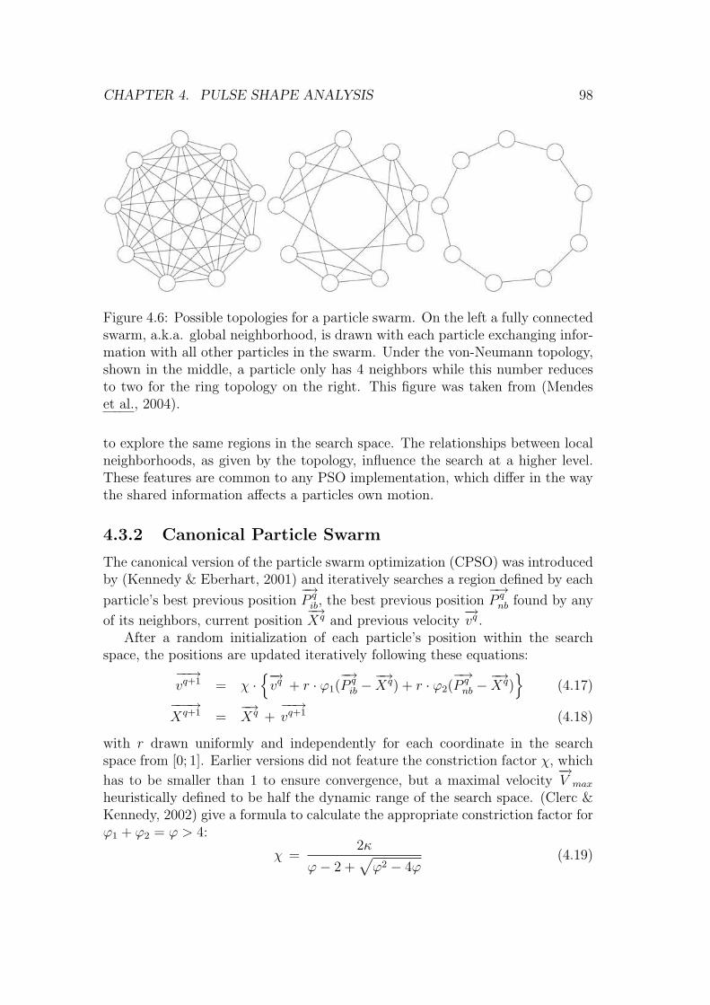
CHAPTER 4. PULSE SHAPE ANALYSIS 98
Figure 4.6: Possible topologies for a particle swarm. On the left a fully connectedswarm, a.k.a. global neighborhood, is drawn with each particle exchanging infor-mation with all other particles in the swarm. Under the von-Neumann topology,shown in the middle, a particle only has 4 neighbors while this number reducesto two for the ring topology on the right. This figure was taken from (Mendeset al., 2004).
to explore the same regions in the search space. The relationships between localneighborhoods, as given by the topology, influence the search at a higher level.These features are common to any PSO implementation, which differ in the waythe shared information affects a particles own motion.
4.3.2 Canonical Particle Swarm
The canonical version of the particle swarm optimization (CPSO) was introducedby (Kennedy & Eberhart, 2001) and iteratively searches a region defined by each
particle’s best previous position−→P q
ib, the best previous position−→P q
nb found by any
of its neighbors, current position−→Xq and previous velocity
−→vq .
After a random initialization of each particle’s position within the searchspace, the positions are updated iteratively following these equations:
−−→vq+1 = χ ·
−→vq + r · ϕ1(
−→P q
ib −−→Xq) + r · ϕ2(
−→P q
nb −−→Xq)
(4.17)
−−−→Xq+1 =
−→Xq +
−−→vq+1 (4.18)
with r drawn uniformly and independently for each coordinate in the searchspace from [0; 1]. Earlier versions did not feature the constriction factor χ, which
has to be smaller than 1 to ensure convergence, but a maximal velocity−→V max
heuristically defined to be half the dynamic range of the search space. (Clerc &Kennedy, 2002) give a formula to calculate the appropriate constriction factor forϕ1 + ϕ2 = ϕ > 4:
χ =2κ
ϕ− 2 +√
ϕ2 − 4ϕ(4.19)

CHAPTER 4. PULSE SHAPE ANALYSIS 99
with κ = 1.0 leading to a slow enough convergence to ensure a thorough searchof the problem domain. On most occasions ϕ1 and ϕ2 are chosen to be equaland the recommended value is 2.05 (Kennedy & Eberhart, 2001) which leads toχ = 0.7298. While a maximal particle velocity is not necessary for convergenceof the presented approach it can still improve the overall performance of thealgorithm.
4.3.3 Fully Informed Particle Swarm
Irrespective of the neighborhood topology, a particle in the CPSO always ex-changes information with just one other particle, the best performing particle inthe neighborhood. However, this does not necessarily mean that no other particlein the neighborhood can provide viable information. In CPSO the most impor-
tant source of variation is the difference between−→P q
ib and−→P q
nb. The analysis in(Clerc & Kennedy, 2002) showed that more than these two information sources,weighted by ϕ1/2, can be utilized since the algorithm is well behaved, in terms ofconvergence and explosion characteristics, if the constriction factor is calculatedwith equation 4.19, irrespective of the number of summands in ϕ =
∑Ni=1 ϕi.
Following this line of thought (Mendes et al., 2004) proposed a change to theupdate equations 4.18:
−−→vq+1 = χ ·
−→vq +
Ni∑
n=1
ϕ · r ·(−→P q
i − −→Xq)
· 1/Ni
(4.20)
−−−→Xq+1 =
−→Xq +
−−→vq+1 (4.21)
with Ni the number of neighbors and−→P q
i the best position found by neighbor i.It is termed fully informed particle swarm (FIPS) since a particle uses informa-tion from all of its neighbors. Another difference to CPSO is that the particlesmemory of its past experience is restricted to the velocity term. Although it ispossible to include the particle in its own neighborhood and hence include its
previous personal best−→P q
ib in the update equations, it was found to be benefi-
cial if−→P q
ib is excluded. The influence of the neighborhood topology on the FIPSperformance was found to be profound (Kennedy & Mendes, 2006). However,a difference in the PSA performance could not be observed for any of the threerecommended topologies. The performance of the two presented particle swarmimplementations on common test functions for evolutionary algorithms was com-pared in (Mendes et al., 2004) and the latter always outperformed the canonicalversion. Consequently only the FIPS version is used for AGATA and it’s perfor-mance for PSA is presented in the next chapter without further discussion of thetopology.
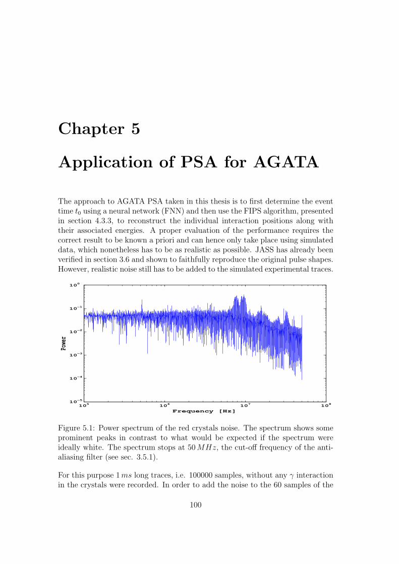
Chapter 5
Application of PSA for AGATA
The approach to AGATA PSA taken in this thesis is to first determine the eventtime t0 using a neural network (FNN) and then use the FIPS algorithm, presentedin section 4.3.3, to reconstruct the individual interaction positions along withtheir associated energies. A proper evaluation of the performance requires thecorrect result to be known a priori and can hence only take place using simulateddata, which nonetheless has to be as realistic as possible. JASS has already beenverified in section 3.6 and shown to faithfully reproduce the original pulse shapes.However, realistic noise still has to be added to the simulated experimental traces.
105
106
107
108
10−5
10−4
10−3
10−2
10−1
100
Frequency [Hz]
Powe
r
Figure 5.1: Power spectrum of the red crystals noise. The spectrum shows someprominent peaks in contrast to what would be expected if the spectrum wereideally white. The spectrum stops at 50MHz, the cut-off frequency of the anti-aliasing filter (see sec. 3.5.1).
For this purpose 1ms long traces, i.e. 100000 samples, without any γ interactionin the crystals were recorded. In order to add the noise to the 60 samples of the
100

CHAPTER 5. APPLICATION OF PSA FOR AGATA 101
simulated signal, correctly scaled with energy, a random starting point within the100000 samples is chosen and the next 60 samples, wrapping around at the end,are added to the signal. Figure 5.1 shows the power spectrum of the noise for oneAGATA crystal ,equipped with the final electronics, featuring some pronouncedpeaks, a clear sign for a non-white spectrum.
In order to gauge the influence the t0 resolution has on the attainable posi-tion resolution the performance of an extensive grid search, i.e. all points in thePSA basis are tested for agreement with the experimental signal, was examinedas a function of normally distributed t0 resolutions. Additionally, the positionresolution is affected by the fact that it is not possible to store the pulse shapesof all 340000 basis points with the full 1ns precision, as given by JASS, due toconstraints on the computer memory to be used by the PSA algorithm. Given
1 2 3 4 5 6 7 8 9 100.5
1
1.5
2
2.5
3
3.5
1 σ T0 Resolution [ns]
Med
ian
3D D
ista
nce
Limit50 keV [5ns]250 keV [5ns]500 keV [5ns]50 keV [2ns]250 keV [2ns]500 keV [2ns]
Figure 5.2: Obtainable position resolution as function of t0 resolution for differentγ energies. The dashed red line marks the performance limit corresponding toa normally distributed position resolution of the X,Y and Z coordinates with5mm (FWHM), just fulfilling the requirements listed in table 4.1. The extensivegrid search is capable of reconstructing the location of a single interaction withthe required precision even if the timing resolution is rather poor independentwhether the basis points are stored with 2ns or 5ns precision.
the ADC’S sampling time of 10ns and the fact that an interpolation of pulseshapes in time adds an unnecessary computational burden on the performancethe only remaining choice is between using a 2ns or 5ns sampling of the basis.This can be considered equivalent to adding additional noise onto the experimen-tal signal. The results for events in the front segment ring are summarized infigure 5.2 showing the median 3D distance between the correct and found solu-tions depending on the timing resolution for both the 2ns and 5ns grids. The

CHAPTER 5. APPLICATION OF PSA FOR AGATA 102
extensive grid search is always within the performance requirements listed in ta-ble 4.1, marked by the dashed red line in the figure. While this might suggesta precise timing resolution is not of importance it has to be kept in mind that,first of all this investigation was conducted using single interactions only andmultiple interaction events will inevitably show a stronger dependence. Secondlythe extensive grid search always finds the best fitting basis point, a feature thatcannot be guaranteed by FIPS as only a subset of all points will be searched. Andlastly, the positive effect a good timing resolution has on the position resolutionis reason enough.
The following section will deal with the neural network used to determine t0,including a description of the data preprocessing, the training and the perfor-mance of the network. The position resolution achieved by FIPS, using differentneighborhood topologies, on single and multiple interaction events will be shownin section 5.2.
5.1 Determination of t0 with Neural Networks
The intended task of the FNN is to determine the event time t0 from the pulseshapes or a subset of the shapes but before the positions are reconstructed bythe FIPS algorithm. In this regard it is important to realize that it is possible topresent too much information to a neural network and unnecessarily complicatingthe matter. Thus some effort has to be spent on which trace, or subsets of traces,should be used before starting the training of the FNN. First of all it suffice todetermine t0 for one trace since all traces are time aligned by the GTS (see sec.F.3). Secondly the core signal has the least dependence on interaction location(see fig. 4.1) and multiplicity1 making it the most suitable trace to be used.
The next point to decide upon is which subset of samples from the core signalis to be presented to the FNN and how to extract these in a reliable manner.Passing the complete trace is deemed unnecessary and unwanted because first ofall the variations of the signal shape with location are much more pronouncedlater in the signal, making it harder for the FNN to find a good generalizationof the signal properties, and secondly because the later stages contain less andless information on t0 (again see fig. 4.1). Since it is rather easy to identify thesample corresponding to t10, i.e. the time until 10% of the total charge have beencollected, in an experimental signal this sample lends itself as a starting pointof the extraction and time alignment of the traces. However, it was found to bebetter to extract the samples using the last sample, counting from the end of thetrace, above the 2σnoise noise level. In the following these will be called the 2σand the t10 sample. In order to investigate the precision of this rough alignmentof the traces, both the t10 and the 2σ sample are always at the same position in
1In contrast to the core signal the shape of a net charge signal is influenced by transientsignals in case of multiple hit segments.
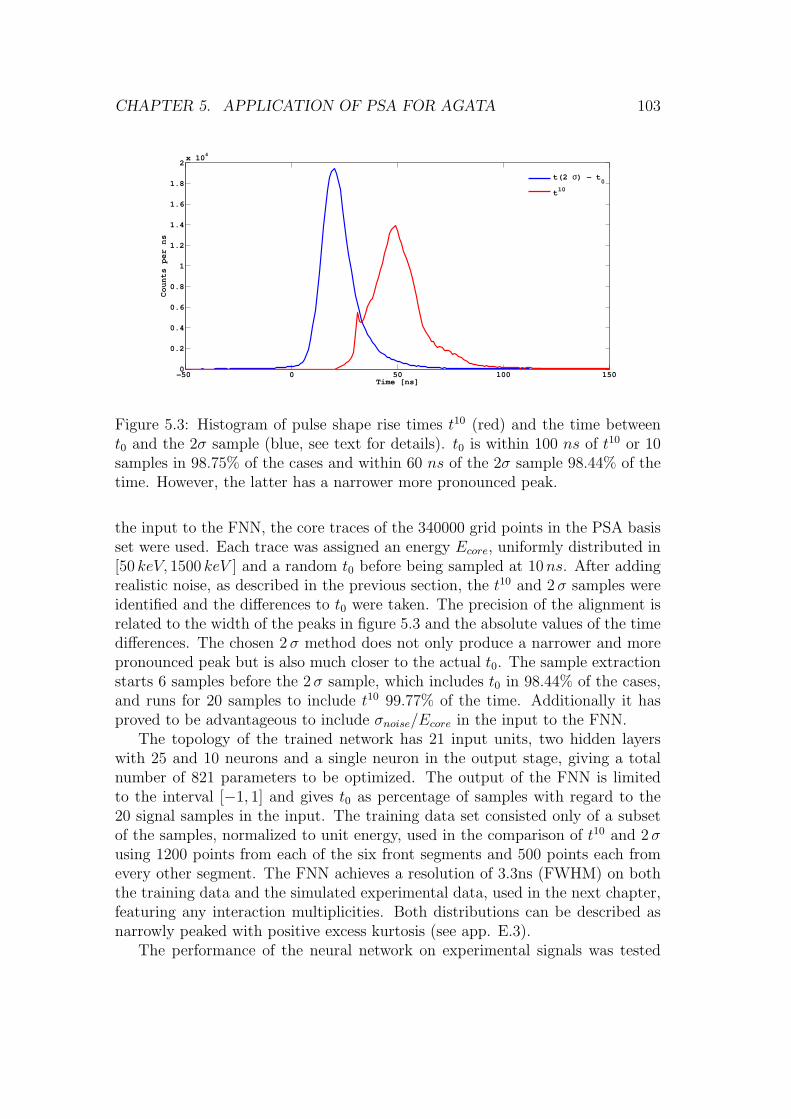
CHAPTER 5. APPLICATION OF PSA FOR AGATA 103
−50 0 50 100 1500
0.2
0.4
0.6
0.8
1
1.2
1.4
1.6
1.8
2x 10
4
Time [ns]
Co
un
ts p
er
ns
t(2 σ) − t0
t 10
Figure 5.3: Histogram of pulse shape rise times t10 (red) and the time betweent0 and the 2σ sample (blue, see text for details). t0 is within 100 ns of t10 or 10samples in 98.75% of the cases and within 60 ns of the 2σ sample 98.44% of thetime. However, the latter has a narrower more pronounced peak.
the input to the FNN, the core traces of the 340000 grid points in the PSA basisset were used. Each trace was assigned an energy Ecore, uniformly distributed in[50 keV, 1500 keV ] and a random t0 before being sampled at 10ns. After addingrealistic noise, as described in the previous section, the t10 and 2σ samples wereidentified and the differences to t0 were taken. The precision of the alignment isrelated to the width of the peaks in figure 5.3 and the absolute values of the timedifferences. The chosen 2σ method does not only produce a narrower and morepronounced peak but is also much closer to the actual t0. The sample extractionstarts 6 samples before the 2σ sample, which includes t0 in 98.44% of the cases,and runs for 20 samples to include t10 99.77% of the time. Additionally it hasproved to be advantageous to include σnoise/Ecore in the input to the FNN.
The topology of the trained network has 21 input units, two hidden layerswith 25 and 10 neurons and a single neuron in the output stage, giving a totalnumber of 821 parameters to be optimized. The output of the FNN is limitedto the interval [−1, 1] and gives t0 as percentage of samples with regard to the20 signal samples in the input. The training data set consisted only of a subsetof the samples, normalized to unit energy, used in the comparison of t10 and 2σusing 1200 points from each of the six front segments and 500 points each fromevery other segment. The FNN achieves a resolution of 3.3ns (FWHM) on boththe training data and the simulated experimental data, used in the next chapter,featuring any interaction multiplicities. Both distributions can be described asnarrowly peaked with positive excess kurtosis (see app. E.3).
The performance of the neural network on experimental signals was tested

CHAPTER 5. APPLICATION OF PSA FOR AGATA 104
−20 −15 −10 −5 0 5 10 15 200
0.1
0.2
0.3
0.4
0.5
0.6
0.7
0.8
0.9
1
Time[ns]
Co
un
ts p
er
ns
Training Datasim. Experiment
Figure 5.4: Timing resolution of the neural network for simulated data.
using the coincident emission of two γ-rays, at 1.17MeV and 1.33MeV , by a60Co source, placed in front of one asymmetric triple cluster. The event selectionprocedure allowed only events in which exactly two crystals detected a γ-ray topass. The network has to determine the same t0 for both hit crystals since theindividual traces are time aligned by the GTS (see sec. F.3). Chance coincidencesare negligible using gates on the line energies and otherwise are limited to only afew % of all events (Bazzacco, 2009). Figure 5.5(b) shows the result including theline gates for all three possible crystal combinations and figure 5.5(a) shows theperformance on all events. The results are summarized in table 5.1 and cannotmatch the performance on simulated data. All distributions are shifted toward
Combination RED-BLUE RED-GREEN GREEN-BLUE
All data 22.7ns 20.4ns 23.3nsLines 9.0ns 8.0ns 9.7ns
Table 5.1: Performance of the trained FNN on experimental data. The resolutionsare quoted as FWHM of the distributions shown in figure 5.5.
negative values hinting at a timing mismatch between the crystals.
5.2 Position Reconstruction with FIPS
In the AGATA PSA framework, as in any real time environment predictabilityplays an important role wherefore a general decision has to be made as to howthe stringent time requirements can be enforced. The two options for PSA are toeither let the PSA algorithm run for a fixed number of iterations or until a certain

CHAPTER 5. APPLICATION OF PSA FOR AGATA 105
−50 −40 −30 −20 −10 0 10 20 30 40 500
5000
10000
15000
Time [ns]
Co
un
ts p
er
ns
RED/BLUERED/GREENGREEN/BLUE
(a) Performance on all data
−50 −40 −30 −20 −10 0 10 20 30 40 500
50
100
150
200
250
300
350
Time [ns]
Co
un
ts p
er
ns
RED/BLUERED/GREENGREEN/BLUE
(b) Performance on line gated data
Figure 5.5: All coincident events and line gated events.

CHAPTER 5. APPLICATION OF PSA FOR AGATA 106
goodness of fit, e.g. a χ2-threshold, is exceeded. There are two problems with thelatter approach. First the χ2-value for a good position resolution in regions ofhigh pulse shape variability, e.g. close to the segment boundaries, is significantlyhigher than in regions of lower sensitivity, e.g. center of a segment. Setting a χ2
threshold large enough to accommodate the highly varying regions allows for poorposition resolutions in the rest of the segment and it is not possible to generallydistinguish the latter from the former simply based on the reconstructed position.Secondly, it fails in terms of predictability as it is not possible to foresee the timetaken to reach the threshold value. Hence the FIPS algorithm will run for afixed number of iterations which will be chosen according to the complexity ofthe hit pattern. In the following the performance on three different hit patterns,namely single segment hits, multiple hit segments with single interactions and twointeractions in one segment, are investigated. The individual results are comparedto those of an extensive grid search, in which all relevant reference signals weresearched. The event time t0 was always determined using the neural networkapproach introduced in section 5.1 since a fit of t0 will increase the computingtimes of the extensive search for multiple interactions way beyond reasonablelevels and prevent the accumulation of results with at least minimal statistics(see e.g. tab. 5.10). The reference signals with 1ns precision were used to givean upper limit on the performance since the demands on computing resourcesprevent such an approach in the experimental environment.
5.2.1 Single Interactions
Obviously, the case of a single γ-ray interaction in a single segment is the easiestpossible scenario with the number of relevant reference signals, i.e. the size of thesearch space, ranging only from 5000 to 12000. The FIPS algorithm was run forjust 10 iterations and took on average 0.7ms, comparing favorably to the 40msto 200ms taken by the extensive grid search (XGS). The performance was testedfor γ-ray energies of 125 keV, 250 keV, 500 keV and 1MeV . Above 500 keV thenoise predominantly influences the timing resolution and only to a lesser extentthe attainable position resolution as the median 3D distance between the correctand found solution of the extensive search only reduces by 0.1mm but the timingresolution is improved by almost 2ns (see tab. 5.2). The lowest tested energy of125 keV is still considerably above the segment energy threshold of 50 keV , thatis used in the hardware DAQ. The preamplifier noise level is 4 keV < 1σ < 6 keV ,depending on the detector. This corresponds to an of 0.08− 0.12 for the normal-ized charge signals at 50 keV and is a factor of two above the average absoluteamplitude of the transient charge signals in directly neighboring segments. Hence,only the net charge signal provides limited information on the interaction loca-tion and large positional errors have to be expected. At an energy of 125 keV atleast some information in the transients is retained and thus presents a reasonablelower limit. The starting positions of the swarm, i.e. the particle positions before
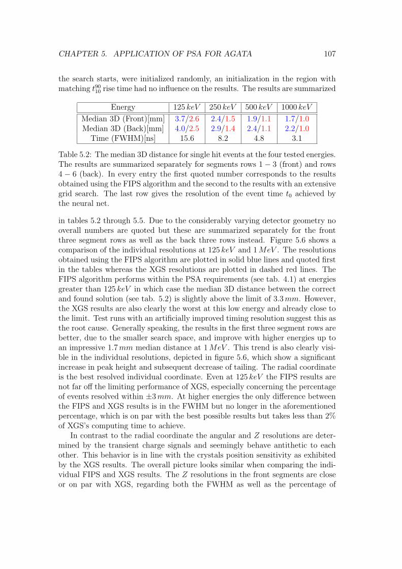
CHAPTER 5. APPLICATION OF PSA FOR AGATA 107
the search starts, were initialized randomly, an initialization in the region withmatching t9010 rise time had no influence on the results. The results are summarized
Energy 125 keV 250 keV 500 keV 1000 keV
Median 3D (Front)[mm] 3.7/2.6 2.4/1.5 1.9/1.1 1.7/1.0Median 3D (Back)[mm] 4.0/2.5 2.9/1.4 2.4/1.1 2.2/1.0
Time (FWHM)[ns] 15.6 8.2 4.8 3.1
Table 5.2: The median 3D distance for single hit events at the four tested energies.The results are summarized separately for segments rows 1 − 3 (front) and rows4 − 6 (back). In every entry the first quoted number corresponds to the resultsobtained using the FIPS algorithm and the second to the results with an extensivegrid search. The last row gives the resolution of the event time t0 achieved bythe neural net.
in tables 5.2 through 5.5. Due to the considerably varying detector geometry nooverall numbers are quoted but these are summarized separately for the frontthree segment rows as well as the back three rows instead. Figure 5.6 shows acomparison of the individual resolutions at 125 keV and 1MeV . The resolutionsobtained using the FIPS algorithm are plotted in solid blue lines and quoted firstin the tables whereas the XGS resolutions are plotted in dashed red lines. TheFIPS algorithm performs within the PSA requirements (see tab. 4.1) at energiesgreater than 125 keV in which case the median 3D distance between the correctand found solution (see tab. 5.2) is slightly above the limit of 3.3mm. However,the XGS results are also clearly the worst at this low energy and already close tothe limit. Test runs with an artificially improved timing resolution suggest this asthe root cause. Generally speaking, the results in the first three segment rows arebetter, due to the smaller search space, and improve with higher energies up toan impressive 1.7mm median distance at 1MeV . This trend is also clearly visi-ble in the individual resolutions, depicted in figure 5.6, which show a significantincrease in peak height and subsequent decrease of tailing. The radial coordinateis the best resolved individual coordinate. Even at 125 keV the FIPS results arenot far off the limiting performance of XGS, especially concerning the percentageof events resolved within ±3mm. At higher energies the only difference betweenthe FIPS and XGS results is in the FWHM but no longer in the aforementionedpercentage, which is on par with the best possible results but takes less than 2%of XGS’s computing time to achieve.
In contrast to the radial coordinate the angular and Z resolutions are deter-mined by the transient charge signals and seemingly behave antithetic to eachother. This behavior is in line with the crystals position sensitivity as exhibitedby the XGS results. The overall picture looks similar when comparing the indi-vidual FIPS and XGS results. The Z resolutions in the front segments are closeor on par with XGS, regarding both the FWHM as well as the percentage of

CHAPTER 5. APPLICATION OF PSA FOR AGATA 108
−15 −10 −5 0 5 10 150
0.5
1
1.5
2
2.5
3
3.5
4
4.5x 10
5
Rf − R
true [mm]
Cou
nts
per m
m
(a) Radial resolution at E = 125 keV .
−15 −10 −5 0 5 10 150
1
2
3
4
5
6
7
8
9x 10
5
Rf − R
true [mm]
Cou
nts
per m
m
(b) Radial resolution at E = 1MeV .
−30 −20 −10 0 10 20 300
2
4
6
8
10
12
14x 10
4
φf − φ
true [deg]
Cou
nts
per d
eg
(c) Angular resolution at E = 125 keV .
−30 −20 −10 0 10 20 300
0.5
1
1.5
2
2.5x 10
5
φf − φ
true [deg]
Cou
nts
per d
eg
(d) Angular resolution at E = 1MeV .
−15 −10 −5 0 5 10 150
0.5
1
1.5
2
2.5
3
3.5
4
4.5x 10
5
Zf − Z
true [mm]
Cou
nts
per m
m
(e) Z resolution at E = 125 keV .
−15 −10 −5 0 5 10 150
1
2
3
4
5
6
7
8x 10
5
Zf − Z
true [mm]
Cou
nts
per m
m
(f) Z resolution at E = 1MeV .
Figure 5.6: Position resolutions for single hit events in the three front segmentrows energies of 125 keV and 1MeV . The results are plotted in solid blue linesfor the FIPS algorithm and in dashed red lines for the extensive search.
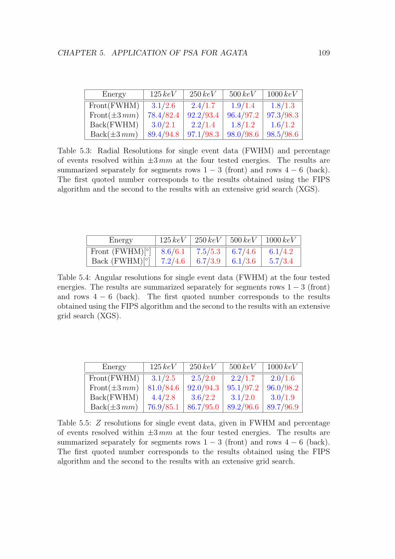
CHAPTER 5. APPLICATION OF PSA FOR AGATA 109
Energy 125 keV 250 keV 500 keV 1000 keV
Front(FWHM) 3.1/2.6 2.4/1.7 1.9/1.4 1.8/1.3Front(±3mm) 78.4/82.4 92.2/93.4 96.4/97.2 97.3/98.3Back(FWHM) 3.0/2.1 2.2/1.4 1.8/1.2 1.6/1.2Back(±3mm) 89.4/94.8 97.1/98.3 98.0/98.6 98.5/98.6
Table 5.3: Radial Resolutions for single event data (FWHM) and percentageof events resolved within ±3mm at the four tested energies. The results aresummarized separately for segments rows 1 − 3 (front) and rows 4 − 6 (back).The first quoted number corresponds to the results obtained using the FIPSalgorithm and the second to the results with an extensive grid search (XGS).
Energy 125 keV 250 keV 500 keV 1000 keV
Front (FWHM)[] 8.6/6.1 7.5/5.3 6.7/4.6 6.1/4.2Back (FWHM)[] 7.2/4.6 6.7/3.9 6.1/3.6 5.7/3.4
Table 5.4: Angular resolutions for single event data (FWHM) at the four testedenergies. The results are summarized separately for segments rows 1 − 3 (front)and rows 4 − 6 (back). The first quoted number corresponds to the resultsobtained using the FIPS algorithm and the second to the results with an extensivegrid search (XGS).
Energy 125 keV 250 keV 500 keV 1000 keV
Front(FWHM) 3.1/2.5 2.5/2.0 2.2/1.7 2.0/1.6Front(±3mm) 81.0/84.6 92.0/94.3 95.1/97.2 96.0/98.2Back(FWHM) 4.4/2.8 3.6/2.2 3.1/2.0 3.0/1.9Back(±3mm) 76.9/85.1 86.7/95.0 89.2/96.6 89.7/96.9
Table 5.5: Z resolutions for single event data, given in FWHM and percentageof events resolved within ±3mm at the four tested energies. The results aresummarized separately for segments rows 1 − 3 (front) and rows 4 − 6 (back).The first quoted number corresponds to the results obtained using the FIPSalgorithm and the second to the results with an extensive grid search.

CHAPTER 5. APPLICATION OF PSA FOR AGATA 110
well resolved events while in the back segments 90% are never obtained and theFWHM are about 1mm larger than in the front. The angular resolutions of theFIPS algorithm are better in the back segments, yet the difference to the XGSresults is about the same in every category.
5.2.2 Multiple Segment Hits
The task of PSA with multiple hit segments becomes more difficult if more thanone segment is hit by a γ-ray. First the size of the search space grows consid-erably (see tab. 4.2) and secondly because overlapping signals in one segmentcan be reproduced by a multitude of reference signal combinations, reducing thatsegments overall information content. Conversely, if none of the segments usedfor PSA are shared between the hit segments each one can and will be analyzedindependently as a single hit event. This leaves two possible general event typesto be investigated. In one case directly neighboring segments have been hit, over-lapping transient with net charge signals, while in the other case a neighboringsegment is shared and only the respective transient signals overlap. In light ofthe plethora of still possible segment combinations only a few exemplary cases,one of each type in the hexagonal and the coaxial region of the detector, arepresented here. Taking the size of the search space into consideration it pays offto initialize the starting positions of the swarm in the region of interest. For thispurpose each segments reference signals have been sorted into 20 equally spacedbins according to the t9010 rise time of the net charge signal. The starting positionsare then chosen randomly from the bins matching the experimental rise time.
Since a search of all reference signal combinations takes at least 600 s perevent (segments A1 and C1) which is far from applicable in the experimentalsetup and furthermore prevents results with high statistics in reasonable time,the extensive search was limited to the reference signals within the appropriaterise time bins. Naturally this leads to a decrease in the obtainable resolutions andin case of segments A1 and C1 with 500 keV γ-ray interactions in each segmentto median 3D distances between the correct and found solutions increases from1.2mm to 2.2mm and from 1.1mm to 2.1mm respectively. However, the averageprocessing time per event is reduced to 1− 2 s which still pales in comparison tothe 3 − 4ms taken by FIPS. Tables 5.6 and 5.7 summarize the results in termsof the median 3D distance between the correct and found solutions for the testedcases at three different energies and for like and unlike energy split.
The attainable and the obtained resolutions for like energy split strongly de-pend on the event type and the region within the detector. In the front seg-ments the rise time limited XGS is only within the PSA requirements for hitsin non-neighboring segments in which case FIPS performs just slightly worse,0.1 − 0.5mm worse median distance, but still within the requirements. Due tothe larger segment size in the back of the crystal the mutual influence on the at-tainable resolutions for hits in directly neighboring segments is smaller and both
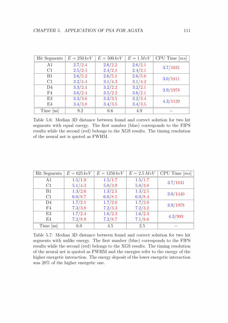
CHAPTER 5. APPLICATION OF PSA FOR AGATA 111
Hit Segments E = 250 keV E = 500 keV E = 1MeV CPU Time [ms]
A1 2.7/2.4 2.6/2.2 2.6/2.13.7/1831
C1 2.5/2.4 2.4/2.1 2.4/2.1B1 2.6/5.2 2.6/5.1 2.6/5.0
3.0/1811C1 3.2/4.4 3.1/4.3 3.1/4.2D4 3.3/2.4 3.2/2.2 3.2/2.1
3.9/1978F4 3.6/2.4 3.5/2.2 3.6/2.1E3 3.3/3.6 3.3/3.5 3.2/3.4
4.3/1129E4 3.4/3.8 3.4/3.5 3.4/3.5
Time [ns] 9.2 6.6 4.9 −
Table 5.6: Median 3D distance between found and correct solution for two hitsegments with equal energy. The first number (blue) corresponds to the FIPSresults while the second (red) belongs to the XGS results. The timing resolutionof the neural net is quoted as FWHM.
Hit Segments E = 625 keV E = 1250 keV E = 2.5MeV CPU Time [ms]
A1 1.5/1.9 1.5/1.7 1.5/1.73.7/1831
C1 5.1/4.3 5.0/3.9 5.0/3.8B1 1.3/2.6 1.3/2.5 1.3/2.5
3.0/1440C1 6.0/8.7 6.0/8.5 6.0/8.4D4 1.7/2.1 1.7/2.0 1.7/2.0
3.9/1978F4 7.3/3.8 7.2/3.3 7.2/3.2E3 1.7/2.4 1.6/2.3 1.6/2.3
4.3/993E4 7.2/8.9 7.2/8.7 7.1/8.6
Time [ns] 6.0 4.5 2.5 −
Table 5.7: Median 3D distance between found and correct solution for two hitsegments with unlike energy. The first number (blue) corresponds to the FIPSresults while the second (red) belongs to the XGS results. The timing resolutionof the neural net is quoted as FWHM and the energies refer to the energy of thehigher energetic interaction. The energy deposit of the lower energetic interactionwas 20% of the higher energetic one.
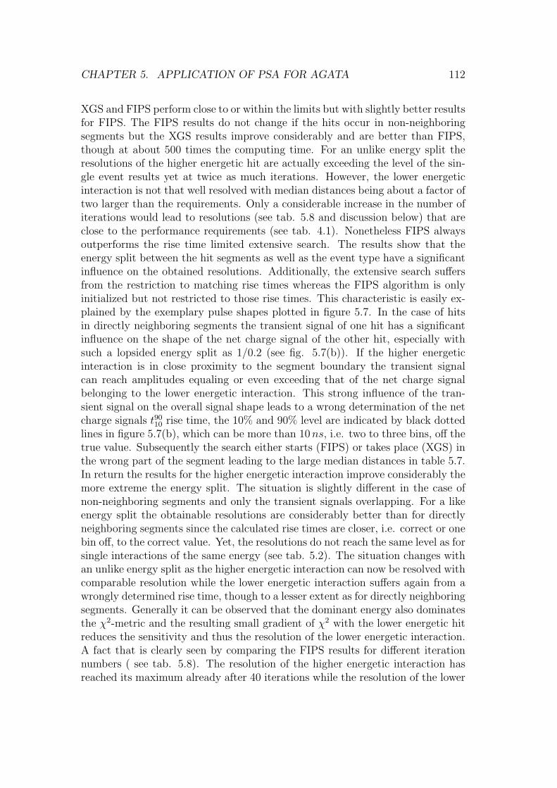
CHAPTER 5. APPLICATION OF PSA FOR AGATA 112
XGS and FIPS perform close to or within the limits but with slightly better resultsfor FIPS. The FIPS results do not change if the hits occur in non-neighboringsegments but the XGS results improve considerably and are better than FIPS,though at about 500 times the computing time. For an unlike energy split theresolutions of the higher energetic hit are actually exceeding the level of the sin-gle event results yet at twice as much iterations. However, the lower energeticinteraction is not that well resolved with median distances being about a factor oftwo larger than the requirements. Only a considerable increase in the number ofiterations would lead to resolutions (see tab. 5.8 and discussion below) that areclose to the performance requirements (see tab. 4.1). Nonetheless FIPS alwaysoutperforms the rise time limited extensive search. The results show that theenergy split between the hit segments as well as the event type have a significantinfluence on the obtained resolutions. Additionally, the extensive search suffersfrom the restriction to matching rise times whereas the FIPS algorithm is onlyinitialized but not restricted to those rise times. This characteristic is easily ex-plained by the exemplary pulse shapes plotted in figure 5.7. In the case of hitsin directly neighboring segments the transient signal of one hit has a significantinfluence on the shape of the net charge signal of the other hit, especially withsuch a lopsided energy split as 1/0.2 (see fig. 5.7(b)). If the higher energeticinteraction is in close proximity to the segment boundary the transient signalcan reach amplitudes equaling or even exceeding that of the net charge signalbelonging to the lower energetic interaction. This strong influence of the tran-sient signal on the overall signal shape leads to a wrong determination of the netcharge signals t9010 rise time, the 10% and 90% level are indicated by black dottedlines in figure 5.7(b), which can be more than 10ns, i.e. two to three bins, off thetrue value. Subsequently the search either starts (FIPS) or takes place (XGS) inthe wrong part of the segment leading to the large median distances in table 5.7.In return the results for the higher energetic interaction improve considerably themore extreme the energy split. The situation is slightly different in the case ofnon-neighboring segments and only the transient signals overlapping. For a likeenergy split the obtainable resolutions are considerably better than for directlyneighboring segments since the calculated rise times are closer, i.e. correct or onebin off, to the correct value. Yet, the resolutions do not reach the same level as forsingle interactions of the same energy (see tab. 5.2). The situation changes withan unlike energy split as the higher energetic interaction can now be resolved withcomparable resolution while the lower energetic interaction suffers again from awrongly determined rise time, though to a lesser extent as for directly neighboringsegments. Generally it can be observed that the dominant energy also dominatesthe χ2-metric and the resulting small gradient of χ2 with the lower energetic hitreduces the sensitivity and thus the resolution of the lower energetic interaction.A fact that is clearly seen by comparing the FIPS results for different iterationnumbers ( see tab. 5.8). The resolution of the higher energetic interaction hasreached its maximum already after 40 iterations while the resolution of the lower

CHAPTER 5. APPLICATION OF PSA FOR AGATA 113
20 30 40 50 60 70−0.02
−0.01
0
0.01
0.02
0.03
0.04
0.05
Time [ns]
No
rma
lize
d C
ha
rge
(a) Shared transient signal for two hit segments with unlike energy de-posits.
25 30 35 40 45 50 55 60 65 70−0.25
−0.2
−0.15
−0.1
−0.05
0
0.05
0.1
Time [ns]
No
rma
lize
d C
ha
rge
Sum signalHigh E.low E.Rise timelimits
(b) Net charge signal of the lower energetic hit for interactions in twodirectly neighboring segments.
Figure 5.7: Net charge and transient signals for two hit segments with unlikeenergy split. The dashed red line corresponds to the signal of the higher energeticinteraction, the dash-dotted green line to the lower energetic interaction and thesolid blue line to the sum of both signals, i.e. the experimental pulse shape. Inboth cases the lower energy was 20% of the higher energy. (a)Transient signal insegment E4, interactions in segments D4 and F4 at a distance of 36mm. (b)Netcharge signal in segment E4 with the higher energetic interaction in E3 at distanceof 24mm.

CHAPTER 5. APPLICATION OF PSA FOR AGATA 114
Hit Segments 20 Iter. 40 Iter. 100 Iter. 200 Iter. XGS
A1 1.5 1.3 1.2 1.2 1.7C1 5.0 4.0 3.4 3.2 3.8B1 1.3 1.1 1.1 1.1 2.5C1 6.0 5.0 4.5 4.3 8.4
CPU Time [ms] 3.9 8.2 14.9 32.9 1800
Table 5.8: Improvement of the median 3D distance between the correct and foundsolution as function of the number of iterations performed by FIPS. The energysplit between the segments was 2500/500 keV .
energetic interaction keeps improving though its biggest step is made by goingfrom 20 to 40 iterations. After 200 iterations the median distance only reducesby a further 0.7mm for hits in directly neighboring segments and by 0.8mm forshared transient signals.
Max. Energy [keV ] A1 B2 C3
500 2.6 3.7 6.11000 2.6 3.7 6.02000 2.5 3.6 6.0
Table 5.9: FIPS performance for three hit segments. The individual energydeposits were 100%, 60% and 30% of the maximal energy.
The case of three hit segments was tested just for a single combination. Theresults are summarized in table 5.9 and show the principle feasibility of analyzingthese types of events. The two most energetic interactions are always resolved ator within the PSA requirements (see tab. 4.1) while the interaction carrying theleast energy is resolved at twice the limit. In the high energy range tested theresults are not affected by the different amount of energy deposits. The averagecomputation time was 12.3ms.
5.2.3 Two interactions in one segment
The first and foremost import task concerning this event type is to find objectivecriteria when to actually search for two hits in the segment. In principle theenergy E1 of the higher energetic interaction can be in the interval 0.5 · Eseg ≤E1 < Eseg, with the lower energy E2 given by the remainder and Eseg the totalenergy deposit in the segment. In practice, however, there is a lower bound forE2 that can be resolved. The lowest possible bound for E2 is 0.1Eseg (Radford,2005) since then its contribution to the signal shape is simply used to fit theinevitable differences between the reference and experimental signals, due to thegrid based approach. Also, the interactions location is no longer restricted but has

CHAPTER 5. APPLICATION OF PSA FOR AGATA 115
only a marginal influence on the overall χ2-value, even in the ideal noiseless case.Applying the segment energy threshold of 50 keV to E2 gives Eseg ≥ 500 keV asa criterion as to when to search for two interactions. For the same reasons asgiven in section 5.2.1 a lower limit of 50 keV for E2 is unrealistic and thus thefollowing minimal energy Emin
2 will be used:
Emin2 = sup 0.1 ∗ Eseg, L, (5.1)
with L to be determined by the test results. Given the results for single interac-tions, it was deduced that L can be no less than 125 keV . Additionally, it has tobe kept in mind that the currently used tracking algorithm packs all individualγ-ray interactions, that lie within 5mm of one another into a single interactionspot.
Hit Segments E = 500 keV E = 1000 keV E = 2.5MeV CPU Time [ms]
B13.3/1.8 3.3/1.4 3.2/1.3
5.9/1.4 · 106
3.5/1.7 3.4/1.4 3.4/1.3
A23.6/1.7 3.5/1.5 3.5/1.2
5.4/2.7 · 106
4.0/1.8 3.9/1.5 3.9/1.3
C44.3/1.3 4.3/1.1 4.3/1.0
5.5/1.1 · 107
4.9/1.2 4.9/1.2 4.8/1.5
Time [ns] 6.0 4.5 2.5 −
Table 5.10: Median 3D distance between found and correct solution for two hitsin one segment with even energy split. The first number (blue) corresponds tothe FIPS results while the second (red) belongs to the XGS results. The timingresolution of the neural net is quoted as FWHM and the energy refers to the totalenergy deposit in the segment.
The results of the test runs are summarized in tables 5.10 - 5.13 and quotethe median 3D distance between the correct and found solutions as obtained bythe FIPS algorithm (red, first number) after 20 iterations and an extensive search(XGS, blue, second number). In both cases the energy split for a given combina-tion of reference signals are calculated by a simple fit algorithm minimizing theχ2-value. Naturally the biggest differences are in terms of computation time asFIPS takes around 5 − 7ms, well within the time constraints, while XGS needs106 − 107ms on a single CPU. Even though the extensive search was run inparallel on 4 CPU’s the latter figure still prevents an accumulation of the samestatistics for XGS as for FIPS. The tests were run for four different energy splits(first interaction with 50/70/80/90%Eseg) between the two interactions at threedifferent segment energies (500/1000/2500 keV ). It is not surprising to see thatthe resolution of the first interaction improves with higher energy split and thatthe resolution of the second interaction improves with higher segment energies

CHAPTER 5. APPLICATION OF PSA FOR AGATA 116
Hit Segments E = 500 keV E = 1000 keV E = 2.5MeV CPU Time [ms]
B12.0/1.4 1.9/1.3 1.9/1.0
5.6/1.4 · 106
4.6/2.8 4.6/2.4 4.5/1.8
A22.1/1.8 2.1/1.2 2.1/0.9
5.2/2.2 · 106
5.2/2.9 5.1/2.3 5.1/1.6
C42.6/1.9 2.6/1.3 2.6/1.0
5.3/1.1 · 107
6.4/3.7 6.3/2.3 6.3/1.8
Time [ns] 6.0 4.5 2.5 −
Table 5.11: Median 3D distance between found and correct solution for two hitsin one segment with energy split 70%/30%. The first number (blue) correspondsto the FIPS results while the second (red) belongs to the XGS results. The timingresolution of the neural net is quoted as FWHM and the energy refers to the totalenergy deposit in the segment.
Hit Segments E = 500 keV E = 1000 keV E = 2.5MeV CPU Time [ms]
B11.6/1.4 1.5/1.2 1.5/1.0
5.3/1.4 · 106
5.8/3.9 5.7/3.3 5.6/2.5
A21.7/1.3 1.6/1.5 1.6/0.9
5.5/2.2 · 106
6.2/4.0 6.1/3.7 6.0/2.5
C42.0/1.2 2.0/1.5 1.9/1.0
5.3/1.2 · 107
7.5/4.3 7.5/2.9 7.4/3.3
Time [ns] 6.0 4.5 2.5 −
Table 5.12: Median 3D distance between found and correct solution for two hitsin one segment with energy split 80%/20%. The first number (blue) correspondsto the FIPS results while the second (red) belongs to the XGS results. The timingresolution of the neural net is quoted as FWHM and the energy refers to the totalenergy deposit in the segment.
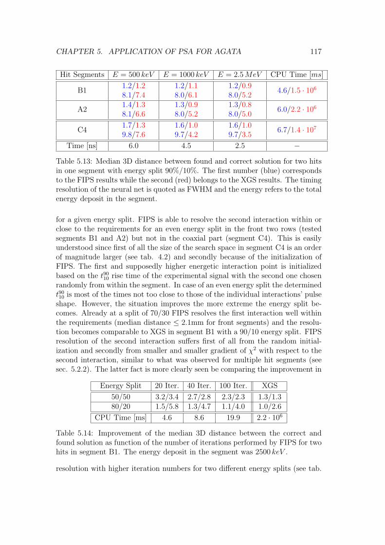
CHAPTER 5. APPLICATION OF PSA FOR AGATA 117
Hit Segments E = 500 keV E = 1000 keV E = 2.5MeV CPU Time [ms]
B11.2/1.2 1.2/1.1 1.2/0.9
4.6/1.5 · 106
8.1/7.4 8.0/6.1 8.0/5.2
A21.4/1.3 1.3/0.9 1.3/0.8
6.0/2.2 · 106
8.1/6.6 8.0/5.2 8.0/5.0
C41.7/1.3 1.6/1.0 1.6/1.0
6.7/1.4 · 107
9.8/7.6 9.7/4.2 9.7/3.5
Time [ns] 6.0 4.5 2.5 −
Table 5.13: Median 3D distance between found and correct solution for two hitsin one segment with energy split 90%/10%. The first number (blue) correspondsto the FIPS results while the second (red) belongs to the XGS results. The timingresolution of the neural net is quoted as FWHM and the energy refers to the totalenergy deposit in the segment.
for a given energy split. FIPS is able to resolve the second interaction within orclose to the requirements for an even energy split in the front two rows (testedsegments B1 and A2) but not in the coaxial part (segment C4). This is easilyunderstood since first of all the size of the search space in segment C4 is an orderof magnitude larger (see tab. 4.2) and secondly because of the initialization ofFIPS. The first and supposedly higher energetic interaction point is initializedbased on the t9010 rise time of the experimental signal with the second one chosenrandomly from within the segment. In case of an even energy split the determinedt9010 is most of the times not too close to those of the individual interactions’ pulseshape. However, the situation improves the more extreme the energy split be-comes. Already at a split of 70/30 FIPS resolves the first interaction well withinthe requirements (median distance ≤ 2.1mm for front segments) and the resolu-tion becomes comparable to XGS in segment B1 with a 90/10 energy split. FIPSresolution of the second interaction suffers first of all from the random initial-ization and secondly from smaller and smaller gradient of χ2 with respect to thesecond interaction, similar to what was observed for multiple hit segments (seesec. 5.2.2). The latter fact is more clearly seen be comparing the improvement in
Energy Split 20 Iter. 40 Iter. 100 Iter. XGS
50/50 3.2/3.4 2.7/2.8 2.3/2.3 1.3/1.380/20 1.5/5.8 1.3/4.7 1.1/4.0 1.0/2.6
CPU Time [ms] 4.6 8.6 19.9 2.2 · 106
Table 5.14: Improvement of the median 3D distance between the correct andfound solution as function of the number of iterations performed by FIPS for twohits in segment B1. The energy deposit in the segment was 2500 keV .
resolution with higher iteration numbers for two different energy splits (see tab.
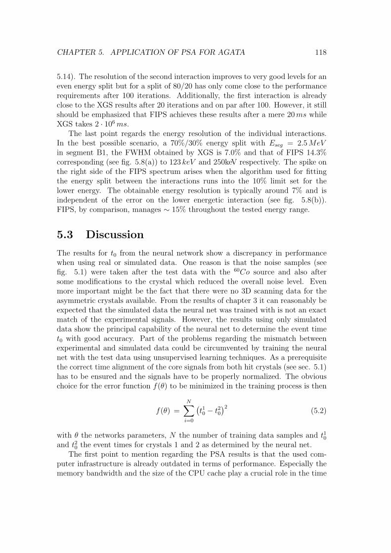
CHAPTER 5. APPLICATION OF PSA FOR AGATA 118
5.14). The resolution of the second interaction improves to very good levels for aneven energy split but for a split of 80/20 has only come close to the performancerequirements after 100 iterations. Additionally, the first interaction is alreadyclose to the XGS results after 20 iterations and on par after 100. However, it stillshould be emphasized that FIPS achieves these results after a mere 20ms whileXGS takes 2 · 106ms.
The last point regards the energy resolution of the individual interactions.In the best possible scenario, a 70%/30% energy split with Eseg = 2.5MeVin segment B1, the FWHM obtained by XGS is 7.0% and that of FIPS 14.3%corresponding (see fig. 5.8(a)) to 123 keV and 250keV respectively. The spike onthe right side of the FIPS spectrum arises when the algorithm used for fittingthe energy split between the interactions runs into the 10% limit set for thelower energy. The obtainable energy resolution is typically around 7% and isindependent of the error on the lower energetic interaction (see fig. 5.8(b)).FIPS, by comparison, manages ∼ 15% throughout the tested energy range.
5.3 Discussion
The results for t0 from the neural network show a discrepancy in performancewhen using real or simulated data. One reason is that the noise samples (seefig. 5.1) were taken after the test data with the 60Co source and also aftersome modifications to the crystal which reduced the overall noise level. Evenmore important might be the fact that there were no 3D scanning data for theasymmetric crystals available. From the results of chapter 3 it can reasonably beexpected that the simulated data the neural net was trained with is not an exactmatch of the experimental signals. However, the results using only simulateddata show the principal capability of the neural net to determine the event timet0 with good accuracy. Part of the problems regarding the mismatch betweenexperimental and simulated data could be circumvented by training the neuralnet with the test data using unsupervised learning techniques. As a prerequisitethe correct time alignment of the core signals from both hit crystals (see sec. 5.1)has to be ensured and the signals have to be properly normalized. The obviouschoice for the error function f(θ) to be minimized in the training process is then
f(θ) =N∑
i=0
(t10 − t20
)2(5.2)
with θ the networks parameters, N the number of training data samples and t10and t20 the event times for crystals 1 and 2 as determined by the neural net.
The first point to mention regarding the PSA results is that the used com-puter infrastructure is already outdated in terms of performance. Especially thememory bandwidth and the size of the CPU cache play a crucial role in the time

CHAPTER 5. APPLICATION OF PSA FOR AGATA 119
−0.2 −0.15 −0.1 −0.05 0 0.05 0.1 0.15 0.20
20
40
60
80
100
120
Ef − E
true [%E
seg]
Co
un
ts p
er
a.u
.
(a) Energy resolution in percent for segment B1 with Eseg = 2.5MeV.
0 5 10 15 20 25 30
−0.2
−0.15
−0.1
−0.05
0
0.05
0.1
0.15
0.2
0.25
3D distance from second interaction [mm]
Ef −
Etr
ue
[%
Ese
g]
(b) Energy resolution as function of the position resolution of the lower energetic hit.
Figure 5.8: Energy resolution in percent for double interactions in segment B1with Eseg = 2.5MeV (a) and its dependence on the position resolution of the lowerenergetic interaction (b). The energy resolution is given in % of the segmentenergy with the solid blue line belonging to the FIPS results and the dashed redline to the XGS results. The histogram of the FIPS results has been scaled topeak height of the XGS spectrum due to its vastly larger statistics.

CHAPTER 5. APPLICATION OF PSA FOR AGATA 120
taken for PSA. Given the pace of development it will soon be possible to do PSAfor two hit segments in less than 1ms, the stated goal for the final array, withoutchanging the algorithm. Concerning the position resolution, FIPS resolves singleinteractions within the limits for positional accuracy for energies greater than125 keV and generally in terms of computing time. Yet, an improvement of thetiming resolution (see tab. 5.2) at the low energies will most likely improve theposition resolution to within requirements. In the case of multiple hit segmentsthe highest energetic interaction is always resolved within the requirements andwill only come close to the limit if the energy split amongst the individual inter-actions is near even. The opposite is true for the lower energetic hit. Previoustries have shown that a random initialization of FIPS starting positions withinthe search space is not fruitful and the resolution of the higher energetic interac-tion clearly profits from the rise time initialization. Hence finding a proper wayto initialize the starting positions for the lower energetic interaction, without theproblems mentioned in section 5.2.2, should be the next topic to be investigated.However, taking into account that the first γ-ray interaction along the scatteringpath is likely to deposit the most energy the rather poor resolutions of the lowerenergetic hit, which do not meet the requirements listed in table 4.1, are not aproblem as long as the tracking performance is not affected. The most demand-ing case of PSA is that of deconvolving two individual γ-ray interactions within asingle segment. The results from section 5.2.3 show that the discussed 10% lowerlimit for E2, i.e. the energy of the lower energetic interaction, is rather optimisticas XGS resolves the second interaction within the PSA requirements only in seg-ment C4 with E2 = 250 keV . Based on these results it can be concluded that thesearch for two interactions in one segment is only feasible for segment energiesEseg ≥ 500 keV and rule 5.1 should be rewritten as:
Emin2 = sup 0.2 ∗ Eseg, 150keV, (5.3)
Regarding FIPS the results can be summarized such that the first interactionlocation is always resolved within the PSA requirements at a 200000 times higherspeed than the extensive search and the resolution of the second location suffersfrom the random initialization and the comparably small gradient of χ2 withrespect to its location. The next topic to investigate in this regard should be tofind a way to initialize the starting positions of FIPS for the second interactionsimilarly close to the correct location as is done for the first interaction. In light ofthe energy resolution it should be tested whether the tracking algorithms actuallybenefits from resolving two hits in the same segment with such a resolution,especially when it comes to separating the interactions of two individual γ-rayshitting the same detector. The probability that the two γ-rays also interact inthe same segment is rather low.

Chapter 6
A Simulated Test Experiment
In the previous chapter the position resolution of the chosen PSA approach wastested for certain isolated event types. However, it is the Doppler correctioncapability of AGATA that is ultimately of interest. While these two issues arerelated to one another there is no possibility to directly transform a given positionresolution into a Doppler-corrected line width. This is especially the case ifother experimental factors, e.g. uncertainties in the target or detector position,contributing to the line width are included. Additional factors influencing thequality of the results are additional, non-active material in the path of the γ-ray and the spectral distribution of the measured γ-rays. In order to get anindication of the actual Doppler correction capabilities of AGATA, early on inthe development phase, a simple test experiment was conducted using the threesymmetric prototype detectors. In the following section the test experiment andthe setup are introduced and in section 6.2 the PSA performance is discussedusing simulated experimental data for reasons outlined below.
6.1 The Test Experiment and Setup
The test experiment was conducted at the 10 MV Tandem accelerator of IKP inCologne and featured a (d,p) reaction in inverse kinematics, using a 48Ti beamat an energy of 100 MeV , impinging on a deuterated titanium target. Thisspecific reaction was chosen as it allowed a simple setup for an event-by-eventdata analysis and a maximization of the excited nucleus’ velocity. The AGATAtriple cryostat was mounted at 90 to the beam axis and as close as possible tothe target (see fig. 6.1(a)) in order to maximize the Doppler-broadening of theobserved γ-ray lines. The direction of the scattered nucleus is reconstructed usinga double sided silicon strip detector (DSSSD), mounted in forward direction,which detects the emitted proton. As this experiment took place before anycomponent of the AGATA DAQ (see sec. 2.2) was operational the used DAQsystem was based on the Multi Branch System (Essel & Kurz, 2000), developed
121

CHAPTER 6. A SIMULATED TEST EXPERIMENT 122
(a) Picture of experimental setup at IKP. (b) Picture of the experimental setup as usedin the GEANT simulation.
Figure 6.1: The setup of the test experiment. (a) The AGATA triple cryostat ison the right and the DSSSD can be seen inside the opened reaction chamber. (b)The triple cryostat is again on the right side of this picture and the DSSSD isrepresented by a green disc. These figures were taken from (Recchia et al., 2009).
at GSI, and the pulses were digitized using XIA-DGF1 cards (14 bit). As aconsequence the experimental pulse shapes are sampled at 25ns instead of 10nsand are also not time aligned. This means that the reference clock for eachchannel was not distributed using the same cable length but in a daisy chain. Sodata from different channels could be off by more than one clock cylce (25ns).Therefore it was decided to use the simulated experimental data, taken from(Recchia et al., 2009), in this thesis in order to get a first impression of AGATAscapabilities. Figure 6.1(b) shows the experimental setup as it has been used inthe GEANT simulation of the experiment. Nonetheless, after some extensivepost-processing of the experimental data, (Recchia et al., 2009) did analyze thedata and report a Doppler corrected line width for the 1382 keV line of 35 keVusing just the crystal locations, 14 keV using the segment locations and 4.8 keVusing an extensive grid search for PSA.
6.2 Performance of PSA
In order to correlate the Doppler-corrected line width with a certain averageposition resolution (Recchia et al., 2009) assumed a normally distributed positionresolution and simply smeared the interaction points with normally distributedpositional errors and took these as the result of the PSA. However, as can beseen from the results in the previous section, either PSA approach delivers resultswith more strongly peaked resolutions as compared to a normal distribution, i.e.
1see http://www.xia.com/DGF_products.html
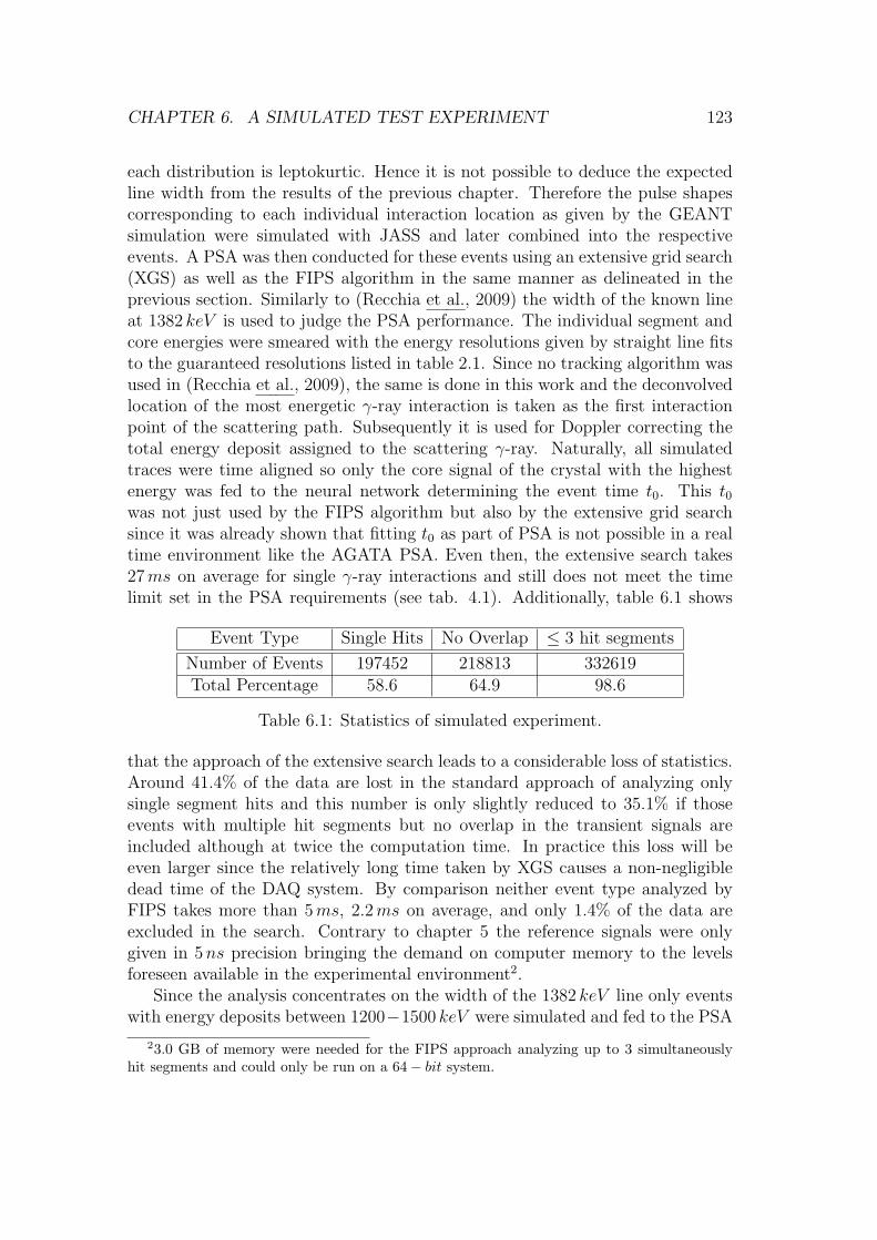
CHAPTER 6. A SIMULATED TEST EXPERIMENT 123
each distribution is leptokurtic. Hence it is not possible to deduce the expectedline width from the results of the previous chapter. Therefore the pulse shapescorresponding to each individual interaction location as given by the GEANTsimulation were simulated with JASS and later combined into the respectiveevents. A PSA was then conducted for these events using an extensive grid search(XGS) as well as the FIPS algorithm in the same manner as delineated in theprevious section. Similarly to (Recchia et al., 2009) the width of the known lineat 1382 keV is used to judge the PSA performance. The individual segment andcore energies were smeared with the energy resolutions given by straight line fitsto the guaranteed resolutions listed in table 2.1. Since no tracking algorithm wasused in (Recchia et al., 2009), the same is done in this work and the deconvolvedlocation of the most energetic γ-ray interaction is taken as the first interactionpoint of the scattering path. Subsequently it is used for Doppler correcting thetotal energy deposit assigned to the scattering γ-ray. Naturally, all simulatedtraces were time aligned so only the core signal of the crystal with the highestenergy was fed to the neural network determining the event time t0. This t0was not just used by the FIPS algorithm but also by the extensive grid searchsince it was already shown that fitting t0 as part of PSA is not possible in a realtime environment like the AGATA PSA. Even then, the extensive search takes27ms on average for single γ-ray interactions and still does not meet the timelimit set in the PSA requirements (see tab. 4.1). Additionally, table 6.1 shows
Event Type Single Hits No Overlap ≤ 3 hit segments
Number of Events 197452 218813 332619Total Percentage 58.6 64.9 98.6
Table 6.1: Statistics of simulated experiment.
that the approach of the extensive search leads to a considerable loss of statistics.Around 41.4% of the data are lost in the standard approach of analyzing onlysingle segment hits and this number is only slightly reduced to 35.1% if thoseevents with multiple hit segments but no overlap in the transient signals areincluded although at twice the computation time. In practice this loss will beeven larger since the relatively long time taken by XGS causes a non-negligibledead time of the DAQ system. By comparison neither event type analyzed byFIPS takes more than 5ms, 2.2ms on average, and only 1.4% of the data areexcluded in the search. Contrary to chapter 5 the reference signals were onlygiven in 5ns precision bringing the demand on computer memory to the levelsforeseen available in the experimental environment2.
Since the analysis concentrates on the width of the 1382 keV line only eventswith energy deposits between 1200−1500 keV were simulated and fed to the PSA
23.0 GB of memory were needed for the FIPS approach analyzing up to 3 simultaneouslyhit segments and could only be run on a 64 − bit system.

CHAPTER 6. A SIMULATED TEST EXPERIMENT 124
algorithm. Figure 6.2 shows the energy spectrum in this interval. The blue dash-dotted line corresponds to the uncorrected, i.e. Doppler shifted, energy deposits.The dashed green line and the solid red line are obtained after correcting for
1200 1250 1300 1350 1400 1450 15000
2000
4000
6000
8000
10000
12000
14000
Energy [keV]
Co
un
ts p
er
0.5
ke
V
UncorrectedFIPSXGS
Figure 6.2: Overlay of uncorrected and Doppler-corrected spectra. The energyspectrum in the analyzed interval is shown before Doppler-correction (blue dash-dotted line), Doppler-corrected after PSA with XGS (dashed green line) andDoppler-corrected after PSA with the FIPS algorithm (solid red line).
the Doppler shift using the results of PSA with either XGS or FIPS respectively.Even without a detailed analysis two important conclusions can already be drawnbased on these spectra. First, FIPS achieves a position resolution that is at leastclose to the XGS results, although multiple hit segments are included. Thisclaim is justified by observing that the increase in analyzed events primarilyleads to an increase in peak amplitude and only marginally to more events inthe background. This gives rise to the second important conclusion that usingFIPS will increase the sensitivity of AGATA considerably and hence positivelyinfluence the detectability of low intensity transitions.
Besides the two already mentioned cases a PSA with FIPS (FIPS singles) wasalso performed with the same event selection used by XGS to make a one-to-one comparison of the two approaches. A close inspection of the spectra alreadyreveals that the peaks are not purely Gaussian in shape but do show some tailing(see fig. 6.4). Therefore the model used to fit the spectra in the region of

CHAPTER 6. A SIMULATED TEST EXPERIMENT 125
interest, 1370 − 1395 keV , included symmetric exponential tails, i.e. a mixtureof a Laplace- and a Gauß-distribution with same peak position µ, plus a linearbackground:
f(x) = N1 · exp(−0.5(x− µ)2/σ2
)+N2 · exp (− |x− µ| /β) + A · x+B. (6.1)
The total peak amplitude is given by N1 +N2 and the width of the distributionsby σ and β respectively. The linear background model has slope A and offsetB. The results can be seen in figure 6.3 and the fitted parameter values aresummarized in table 6.2. The goodness of fit can be assessed using the R2 value
1370 1375 1380 1385 1390 1395 14000
1000
2000
3000
4000
5000
6000
7000
8000
Energy [keV]
Co
un
ts p
er
0.5
ke
V
Fitted Model Data
(a) Fit to XGS peak.
1370 1375 1380 1385 1390 1395 14000
1000
2000
3000
4000
5000
6000
Energy [keV]
Co
un
ts p
er
0.5
ke
V
Fitted Model Data
(b) Fit to FIPS single
1370 1375 1380 1385 1390 1395 14000
2000
4000
6000
8000
10000
12000
14000
Energy [keV]
Co
un
ts p
er
0.5
ke
V
Fitted Model Data
(c) Fit to FIPS all.
1370 1375 1380 1385 1390 1395 1400−0.2
0
0.2
0.4
0.6
0.8
1
1.2
Energy [keV]
No
rma
lize
d C
ou
nts
pe
r 0
.5 k
eV
XGSall FIPS single FIPS
(d) Comparison of background subtracted nor-malized peaks.
Figure 6.3: Fits of model 6.1 to Doppler-corrected spectra after PSA with (a)XGS, (b) FIPS single segment hits and (c) FIPS with up to three hit segments.The extracted peak spectra were superimposed onto each other after subtrac-tion of the fitted background contributions and subsequent normalization to unitamplitude (d).
(0 ≤ R2 ≤ 1) which is a function of the squared residuals and the variance of thedata. It is a measure for the correlation between the data and the model with1 indicating a perfect correlation. The adjusted R2 values take the degrees offreedom in the same manner into account as is known for χ2. In case of the fitted

CHAPTER 6. A SIMULATED TEST EXPERIMENT 126
Parameter XGS FIPS singles FIPS all
N1 3303 ± 514 3065 ± 245 5654 ± 446N2 4221 ± 551 2927 ± 297 7091 ± 588µ 1382+0.2
−0.1 1382+0.2−0.1 1382+0.2
−0.1
σ 1.57 ± 0.1 1.68 ± 0.07 1.55 ± 0.06β 1.2+0.2
−0.1 1.5 ± 0.2 1.96 ± 0.12A −2.8 ± 2.3 −1.5 ± 1.5 −5.7 ± 2.8B 4112 ± 3186 2339 ± 2090 8271 ± 3918
Adj. R2 0.99 0.99 0.99
FWHM [mm] 2.8 3.3 3.4avg. CPU Time [ms] 27 0.8 2.2
Table 6.2: Parameters of the fitted peak model and goodness of fit for theDoppler-corrected peaks. The FWHM is calculated from the background-subtracted spectra. The quoted errors correspond to the 95% confidence level.
model they are close to unity for each fit and indicate a good match with theexperimental data. All three approaches reconstruct the correct peak position of1382 keV with the same small uncertainties. On the other hand the widths of theLaplacian distributions show a sizable difference while the widths of the Gaussiandistributions are comparable for each of the three cases. Yet the considerabledifferences in the contributions of the two distributions to the individual peakshapes make a comparison of their widths in terms of overall peak resolutionnot meaningful. Therefore the FWHM of each peak was calculated from thespectra after subtraction of the fitted background model. As can be expected XGSproduces the narrowest peak with 2.8 keV FWHM but the resolution of FIPS isonly 0.5 − 0.6keV wider. The remarkable result however is that the resolutionof FIPS is practically the same independent of whether multiple segment hitsare included or not (see fig. 6.3(d)). The only observable differences are theslightly stronger tails for multiple segment hits. Generally speaking the fit resultsconfirm the earlier claim of comparable resolutions not only by the numbers butalso because the peak amplitude (N1 + N2) increases by the same factor as thenumber of analyzed events, i.e. 1.7.
6.3 Discussion
An interesting question not yet discussed is whether the PSA algorithms resolvethe energetic barycenter of multiple interactions within a segment with the sameresolution as for the true single hits analyzed in the previous chapter. Figure6.4 shows the resolutions of the radial, angular and Z coordinate as well as thedistance of the found location from the barycenter for the analyzed simulated

CHAPTER 6. A SIMULATED TEST EXPERIMENT 127
experimental data. The solid blue line always corresponds to the results of the
−10 −5 0 5 100
1
2
3
4
5
6
7x 10
4
Rf − R
true [mm]
Cou
nts
per
mm
(a) Radial resolution of single segment hits.
−30 −20 −10 0 10 20 300
2000
4000
6000
8000
10000
12000
14000
16000
18000
φf − φ
true [deg]
Cou
nts
per
deg
(b) Angular resolution of single segment hits.
−10 −5 0 5 100
1
2
3
4
5
6x 10
4
Zf − Z
true [mm]
Cou
nts
per
mm
(c) Z resolution of single segment hits.
0 2 4 6 8 100
1
2
3
4
5
6x 10
4
Distance [mm]
Co
un
ts p
er
0.5
mm
(d) 3D distance from correct location.
Figure 6.4: Position resolution of the energetic barycenter for single segment hitsin the simulated experimental data. The solid blue line corresponds to the resultsof the FIPS algorithm and the dashed red line to the results of XGS.
FIPS algorithm and the dashed red line to the results of XGS. In all cases theresolutions are as if a true single interaction occurred at the energetic barycenter,important to know for the tracking algorithms (compare table 6.3 with tables5.2-5.5). Interestingly the individual distributions coincide with one another forpoorly resolved events, e.g. errors on Z greater than ±5mm or for distancesgreater than 8mm. The FIPS algorithm manages to get close to the correctsolution rather quickly but does not always end up at that location leading tohigher amplitudes around the peaks as opposed to the results with XGS.
As was already briefly mentioned it is possible for FIPS to analyze events upto a segment multiplicity of three and stay within the performance requirements

CHAPTER 6. A SIMULATED TEST EXPERIMENT 128
Algorithm Radial [mm] Z [mm] Angular [] Med. 3D distance [mm]
XGS 1.3 1.4 4.0 1.4FIPS 1.7 1.8 6.1 1.8
Table 6.3: Position resolution of XGS and FIPS for single segment hits in thesimulated experiment.
set for PSA (see tab. 4.1). The γ-ray interaction with the highest energy deposit,also likely the first interaction used for the Doppler-correction, is practically aswell resolved as if it were a single interaction. Thus the energy resolution is notadversely affected compared to single segment hits analyzed with FIPS. This is animportant advantage over XGS since the resulting increase in analyzable eventsas well as the higher speed of FIPS lead to a higher resolving power for AGATA,outweighing the effects of the slightly poorer energy resolution (see eqn. 1.3).
Finally, it can be concluded, that the chosen approach to PSA of determiningthe event time t0 with a neural net and subsequent reconstruction of the inter-actions locations with the FIPS algorithm works well within the performancerequirements (see 4.1). The capability of FIPS to accurately resolve the firstinteraction location independent of the segment multiplicity is crucial to harnessthe full resolving power offered by AGATA.

Appendix A
Moments of the scanning
distributions
In the following tables the higher order moments of the distributions plotted infigures 3.22 through 3.28 are listed. The values, from left to right, belong toparameter set A, set B and the simulated data and are given in the same colorsas in the above mentioned figures.
Moment Row 1 Row 2 Row 3 Row 4
γ1 −0.0/0.1/−1.4 0.6/0.9/−0.8 0.2/0.4/−2.2 0.0/−0.0/−0.2γ2 3.6/0.6/81.0 3.5/3.2/58.7 4.5/9.3/56.1 6.0/9.1/48.5
Row 5 Row 6 Allγ1 0.8/1.0/−0.3 1.3/1.2/−2.6 0.2/0.3/−1.6γ2 7.6/9.0/39.8 18.2/16.2/44.2 5.4/4.5/63.3
Table A.1: Moments of X distributions.
Moment Row 1 Row 2 Row 3 Row 4
γ1 −0.2/−0.1/−0.4 0.0/−0.3/0.3 −0.1/−0.4/0.6 −0.1/−0.4/0.4γ2 0.8/0.6/61.1 3.5/3.2/35.4 2.5/5.7/28.6 3.9/7.0/25.6
Row 5 Row 6 Allγ1 −0.2/−0.5/0.4 −0.9/−0.9/−0.2 −0.2/−0.2/0.1γ2 7.5/6.6/35.8 14.0/11.6/35.1 2.9/3.2/48.5
Table A.2: Moments of Y distributions.
129

APPENDIX A. MOMENTS OF THE SCANNING DISTRIBUTIONS 130
Moment Row 1 Row 2 Row 3 Row 4
γ1 0.9/1.0/1.0 0.2/0.1/2.5 0.0/0.1/−1.0 −0.1/−0.1/−1.3γ2 4.9/4.6/4.2 0.1/−0.2/17.2 0.2/0.6/15.1 0.7/1.2/19.6
Row 5 Row 6 Allγ1 −0.1/−0.1/−1.4 0.0/−0.1/−0.2 0.2/0.2/−0.2γ2 1.0/1.3/11.3 −0.8/−0.7/6.9 2.4/2.6/15.0
Table A.3: Moments of Z distributions.
Moment Row 1 Row 2 Row 3 Row 4
γ1 0.3/0.4/−6.6 0.3/0.3/6.0 0.4/0.2/3.0 0.9/1.3/3.6γ2 0.8/0.5/83.6 10.1/12.5/69.9 14.5/21.1/44.9 13.3/21.6/38.8
Row 5 Row 6 Allγ1 2.4/2.7/4.1 4.1/4.2/4.9 0.5/0.1/−0.9γ2 24.3/32.2/37.7 35.2/37.9/54.3 7.8/6.1/74.1
Table A.4: Moments of R distributions.
Moment Row 1 Row 2 Row 3 Row 4
γ1 7.4/7.3/4.7 4.7/5.7/3.6 2.5/3.2/5.3 1.9/2.3/3.2γ2 69.7/60.3/80.6 53.4/44.7/87.1 40.5/37.8/95.3 43.2/41.2/88.2
Row 5 Row 6 Allγ1 6.5/6.8/1.5 0.4/6.7/1.4 3.9/4.5/3.8γ2 88.8/64.9/78.9 136.1/107.0/72.6 53.2/47.9/83.7
Table A.5: Moments of ϕ distributions.
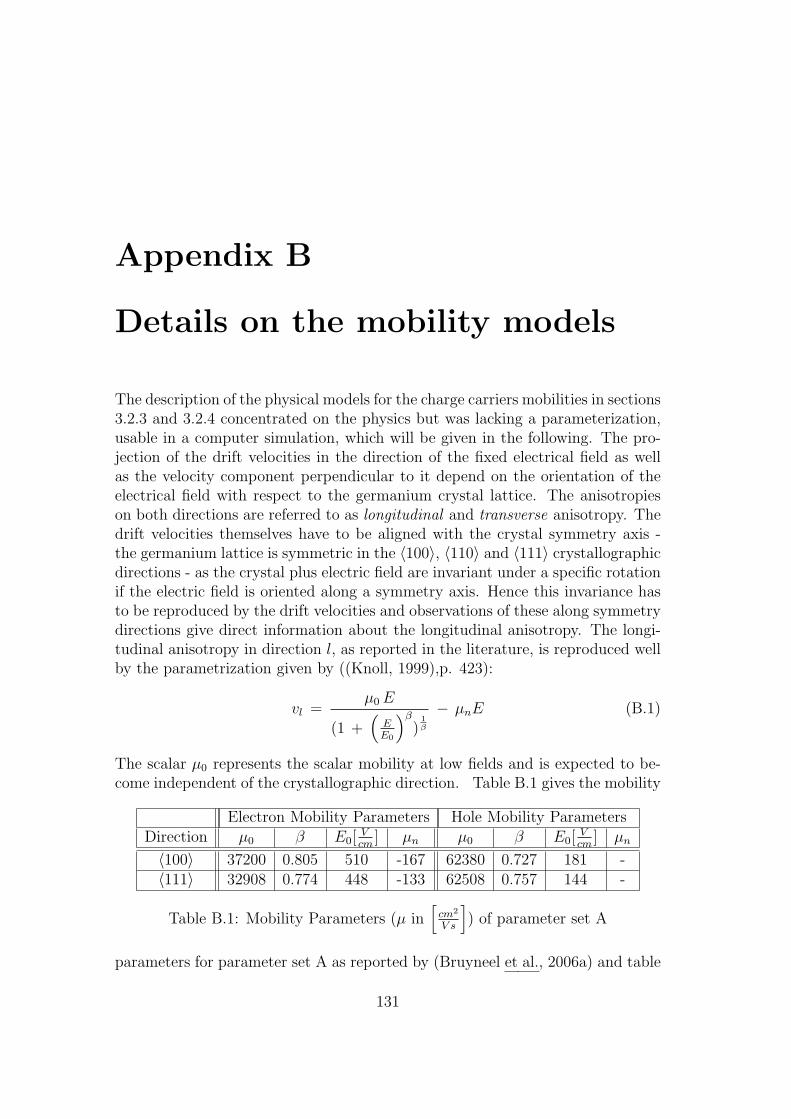
Appendix B
Details on the mobility models
The description of the physical models for the charge carriers mobilities in sections3.2.3 and 3.2.4 concentrated on the physics but was lacking a parameterization,usable in a computer simulation, which will be given in the following. The pro-jection of the drift velocities in the direction of the fixed electrical field as wellas the velocity component perpendicular to it depend on the orientation of theelectrical field with respect to the germanium crystal lattice. The anisotropieson both directions are referred to as longitudinal and transverse anisotropy. Thedrift velocities themselves have to be aligned with the crystal symmetry axis -the germanium lattice is symmetric in the 〈100〉, 〈110〉 and 〈111〉 crystallographicdirections - as the crystal plus electric field are invariant under a specific rotationif the electric field is oriented along a symmetry axis. Hence this invariance hasto be reproduced by the drift velocities and observations of these along symmetrydirections give direct information about the longitudinal anisotropy. The longi-tudinal anisotropy in direction l, as reported in the literature, is reproduced wellby the parametrization given by ((Knoll, 1999),p. 423):
vl =µ0E
(1 +(
EE0
)β
)1β
− µnE (B.1)
The scalar µ0 represents the scalar mobility at low fields and is expected to be-come independent of the crystallographic direction. Table B.1 gives the mobility
Electron Mobility Parameters Hole Mobility ParametersDirection µ0 β E0[
Vcm
] µn µ0 β E0[Vcm
] µn
〈100〉 37200 0.805 510 -167 62380 0.727 181 -〈111〉 32908 0.774 448 -133 62508 0.757 144 -
Table B.1: Mobility Parameters (µ in[
cm2
V s
]
) of parameter set A
parameters for parameter set A as reported by (Bruyneel et al., 2006a) and table
131

APPENDIX B. DETAILS ON THE MOBILITY MODELS 132
Electron Mobility Parameters Hole Mobility ParametersDirection µ0 β E0[
Vcm
] µn µ0 β E0[Vcm
] µn
〈100〉 40180 0.72 493 589 66333 0.744 181 -〈111〉 42420 0.87 251 62 107270 0.580 100 -
Table B.2: Mobility Parameters (µ in[
cm2
V s
]
) of parameter set B.
B.2 for set B as reported by (Mihailescu et al., 2000; Reggiani et al., 1977). Inthe following the parameterization of the mobility models for the electrons andholes, as described in sections 3.2.3 and 3.2.4, are presented using equation B.1.
B.1 Parameterization of the electron model
In the case of the electron mobility it is rather straightforward to relate theexperimentally accessible parameters, listed in tables B.1 and B.2, to the modeldescribed in section 3.2.3. Identifying the effective mobility µ∗ in equation 3.15with the v100 drift velocity and utilizing the fact that all four electron valleysare equally populated if the electric field ~E is aligned with the 〈100〉 direction,equation 3.15 can be rearranged and yields the following relation:
µ∗(E) =v100(E/Γ0)
Γ0E. (B.2)
The constant Γ0 = 2.888 is defined by the mass tensor elements in equation 3.13.The only remaining question now concerns the weights ni in equation 3.15 for anarbitrarily oriented field. If the field is oriented along the 〈111〉 direction of valley1 the remaining three valleys are equally populated with an amount of (1−n1)/3and equation 3.15 an be rearranged to
n1 =v111(E) − Γ2
2µ∗(Γ2E) · E
Γ21µ
∗(Γ1E) · E − Γ22µ
∗(Γ2E) · E . (B.3)
The constants Γ1 = 0.7809 and Γ2 = 3.305 are again given by the mass tensorelements in equation 3.13. The weights ni can now be calculated with the helpof n1 and the relative field strengths in each of the four valleys obeying theconstraint that
∑4i=1 ni = 1. Thus the mobility of the electrons is fully specified
in any direction using only the mobilities in the 〈100〉 and 〈111〉 directions.
B.2 Parameterization of the hole model
While the numerical evaluation of the three dimensional integral in equation 3.19is possible, it is too time consuming to be used in a pulse shape simulation. How-ever, the k dependence can be integrated over explicitly and only a 2D integral

APPENDIX B. DETAILS ON THE MOBILITY MODELS 133
has to be approximated. In the following the constant factor ~/√
2mkbTh in equa-tion 3.16 will be absorbed into the definition of k and k0, which can in turn beinterpreted as the solid-state equivalent to the Mach number in fluid dynamics.Rewriting equation 3.19 in Cartesian coordinates gives:
vx(−→ko) =
v100(ko)
n(k0)
∫ 2π
0
∫ π
0
X(θ, ϕ) exp[k2
0(R2 − 1)
]I3(koR) sin(θ)dθdϕ
vy(−→ko) =
v100(ko)
n(k0)
∫ 2π
0
∫ π
0
Y (θ, ϕ) exp[k2
0(R2 − 1)
]I3(koR) sin(θ)dθdϕ
vz(−→ko) =
v100(ko)
n(k0)
∫ 2π
0
∫ π
0
Z(θ, ϕ) exp[k2
0(R2 − 1)
]I3(koR) sin(θ)dθdϕ.(B.4)
The normalization constant n(k0) can be found by identifying vx(k0, θ = π/2, ϕ =0) with the v100(k0) mobility. The vector k [X(θ, ϕ), Y (θ, ϕ), Z(θ, ϕ)] is the gra-
dient−→∇kǫ(~k) (see eqn. 3.3) and R is an abbreviation for the cosine of the angle
between ~k and−→k0 :
R(θ, ϕ, θ0, ϕ0) =~k
k·~k0
k0
= sin(θ0) sin(θ)cos(ϕ− ϕ0) + cos(θ0) cos(θ). (B.5)
The function I3(koR) contains the complete k-dependence of the integration andbelongs to a family of integrals given by:
In(x) =
∫ ∞
0
kn exp(−(k − x)2)dk
with the general solution:
In(x) =1
2
n∑
m=0
(n
m
)
xn−m
Γ(m+ 1
2) + (−1)m sgn(x) · γ(m+ 1
2, x2)
.(B.6)
The general solution is obtained by substituting y = k − x and by expanding(y+x)n in its binomial form and states that the integral can be expanded in termof the complete and incomplete gamma functions, i.e. Γ(x) and γ(x).
B.2.1 A useful approximation
In order to facilitate the use of the model in a pulse shape simulation (Bruyneelet al., 2006a) developed a fit function for the integrals in equations B.4 and
provide a good approximation for k0 < 3. Using the−→ko(k0, θ0, ϕ0) components of
the mean wave vector, which is aligned with the electrical field−→E (E, θ0, ϕ0) (see
sec. 3.2.4), the velocities can be expressed as:
vr = v100(E)[1 − Λ(k0)(sin(θ0)
4 sin(2ϕ0)2 + sin(2θ0)
2)]
vθ = v100(E)Ω(k0)[2 sin(θ0)
3 cos(θ0) sin(2ϕ0)2 + sin(4θ0)
]
vϕ = v100(E)Ω(k0) sin(θ0)3 sin(4ϕ0). (B.7)
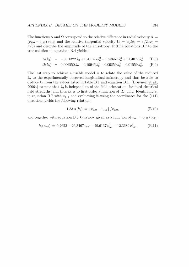
APPENDIX B. DETAILS ON THE MOBILITY MODELS 134
The functions Λ and Ω correspond to the relative difference in radial velocity Λ =(v100 − v110) /v100 and the relative tangential velocity Ω = vϕ(θ0 = π/2, ϕ0 =π/8) and describe the amplitude of the anisotropy. Fitting equations B.7 to thetrue solution in equations B.4 yielded:
Λ(k0) = −0.01322 k0 + 0.41145 k20 − 0.23657 k3
0 + 0.04077 k40 (B.8)
Ω(k0) = 0.006550 k0 − 0.19946 k20 + 0.09859 k3
0 − 0.01559 k40. (B.9)
The last step to achieve a usable model is to relate the value of the reducedk0 to the experimentally observed longitudinal anisotropy and thus be able todeduce k0 from the values listed in table B.1 and equation B.1. (Bruyneel et al.,2006a) assume that k0 is independent of the field orientation, for fixed electricalfield strengths, and thus k0 is to first order a function of |E| only. Identifying vr
in equation B.7 with v111 and evaluating it using the coordinates for the 〈111〉directions yields the following relation:
1.33 Λ(k0) = v100 − v111 /v100, (B.10)
and together with equation B.8 k0 is now given as a function of vrel = v111/v100:
k0(vrel) = 9.2652 − 26.3467 vrel + 29.6137 v2rel − 12.3689 v3
rel. (B.11)

Appendix C
Plane Equations and Hesse’s
Normal Form
The mathematical definition of a plane is quite simple. A plane consists of allpoints P (x, y, z) ∈ R
3 that satisfy the following equation:
A · x+B · y + C · z +D = 0. (C.1)
The plane equation is written in the so-called component form. A,B and C are
the non-normalized components of the plane’s normal vector−→N(A,B,C). D is
zero only if the origin is part of the plane. The direction cosines of−→N are:
cosα =A√
A2 +B2 + C2, cos β =
B√A2 +B2 + C2
, cos γ =C√
A2 +B2 + C2.
(C.2)Multiplying equation C.1 with the normalization factor:
±µ =1∣∣∣−→N
∣∣∣
=1√
A2 +B2 + C2(C.3)
leads to Hesse’s normal form of the plane equation:
cosα · x+ cos β · y + cos γ · z − p = 0, (C.4)
with p being the distance of the plane from the origin. The sign of µ has to bechosen opposite to that of D.
On many technical occasions, like the specification of the AGATA crystals(see sec. 3.2.1), a plane is specified by giving three points P (x1−3, y1−3, z1−3)that are required to lie on the plane. The plane is thus uniquely defined and thecomponent form is given by:
∣∣∣∣∣∣
x− x1 y − y1 z − z1
x2 − x1 y2 − y1 z2 − z1
x3 − x1 y3 − y1 z3 − z1
∣∣∣∣∣∣
= 0. (C.5)
135
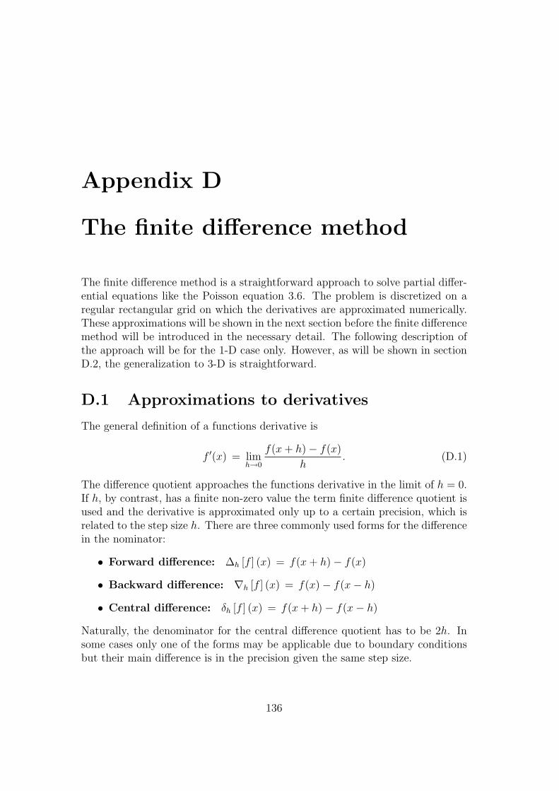
Appendix D
The finite difference method
The finite difference method is a straightforward approach to solve partial differ-ential equations like the Poisson equation 3.6. The problem is discretized on aregular rectangular grid on which the derivatives are approximated numerically.These approximations will be shown in the next section before the finite differencemethod will be introduced in the necessary detail. The following description ofthe approach will be for the 1-D case only. However, as will be shown in sectionD.2, the generalization to 3-D is straightforward.
D.1 Approximations to derivatives
The general definition of a functions derivative is
f ′(x) = limh→0
f(x+ h) − f(x)
h. (D.1)
The difference quotient approaches the functions derivative in the limit of h = 0.If h, by contrast, has a finite non-zero value the term finite difference quotient isused and the derivative is approximated only up to a certain precision, which isrelated to the step size h. There are three commonly used forms for the differencein the nominator:
• Forward difference: ∆h [f ] (x) = f(x+ h) − f(x)
• Backward difference: ∇h [f ] (x) = f(x) − f(x− h)
• Central difference: δh [f ] (x) = f(x+ h) − f(x− h)
Naturally, the denominator for the central difference quotient has to be 2h. Insome cases only one of the forms may be applicable due to boundary conditionsbut their main difference is in the precision given the same step size.
136

APPENDIX D. THE FINITE DIFFERENCE METHOD 137
D.1.1 Errors of the approximations
The above approximations can equivalently be deduced by expanding f(x) in aTaylor series to first order and solving for f ′(x). According to Taylor’s theoremthe error of such an approximation is determined by the remainder termRn(x+h),written in the Lagrange form, ((Bronstein, 2000), p. 434):
Rn(x+ h) =f (n+1)(ξ)
(n+ 1)!· hn+1, with x < ξ < x+ h (D.2)
The error of the forward difference is thus:
f(x+ h) = f(x) + f ′(x) · h+f ′′(ξ)
2!· h2
f(x+ h) − f(x)
h= f ′(x) +
f ′′(ξ)
2!· h
f(x+ h) − f(x)
h= f ′(x) +O(h). (D.3)
Analogously, the error of the backward difference is O(h). In order to calculatethe error of the central difference the Taylor series has to be expanded up to thirdorder twice, once for f(x + h) and once for f(x − h), and subtracted from oneanother. In this case the second derivatives cancel each other (see eqns. D.4 andD.5) and the remainder term is given by the third derivative leading to errors oforder h2.
D.1.2 Higher order derivatives
The finite difference approximations to higher order derivatives can be derived insimilar fashion by expanding f(x) to higher order Taylor series. In the followingthe central difference approximation to the second derivative of f(x) will bederived as an example. The fourth order Taylor expansions for both f(x + h)and f(x− h) are:
f(x+ h) = f(x) + f ′(x)h+h2f ′′(x)
2+h3f (3)(x)
6+h4f (4)(x)
24(D.4)
f(x− h) = f(x) − f ′(x)h+h2f ′′(x)
2− h3f (3)(x)
6+h4f (4)(x)
24. (D.5)
Adding both equations eliminates the odd derivatives and solving for f ′′(x) yields:
f ′′(x) =f(x+ h) − 2f(x) + f(x− h)
h2− 2h2f (4)(x)
24. (D.6)
The remainder term is again of order h2. In fact, the approximation errors forthe higher order derivatives will always be the same as for the first derivatives(see sec. D.1.1).

APPENDIX D. THE FINITE DIFFERENCE METHOD 138
More generally, the nth-order forward, backward, and central differences arerespectively given by:
∆nh [f ] (x) =
n∑
i=0
(−1)i
(n
i
)
f(x+ (n− i) · h) (D.7)
∇nh [f ] (x) =
n∑
i=0
(−1)i
(n
i
)
f(x− i · h) (D.8)
δnh [f ] (x) =
n∑
i=0
(−1)i
(n
i
)
f(x+ (n/2 − i) · h) (D.9)
D.2 Solving Partial Differential Equations
The above presented finite difference approximations can be used to solve partialdifferential equations. In the following the basic approach undertaken will beexplained using the one dimensional Poisson equation:
Φ′′(x) = −ρ(x)εε0
, x ∈ [0, 1], (D.10)
with space charge distribution ρ(x), as an example.As a first step, equation D.10 is discretized on a regular grid of N points. The
ith grid point therefore has the coordinate xi = i·h = xi−1+h with h = 1/N . Thevalues Φ(0) and Φ(1) are given by boundary conditions, such as fixed voltages atthe electrodes or fixed values for the electric fields. Using equation D.6, the lefthand side of equation D.10 is approximated on every grid point:
Φ(xi+1) − 2 Φ(xi) + Φ(xi−1)
h2= −ρ(xi)
εε0
. (D.11)
This results in a linear system of N − 2 equations which has to be solved. Thevarious finite difference methods differ only in the way this system of equationsis solved.
The generalization to the three dimensional case is straightforward. Giventhat ∇ = ∂2
∂x2 + ∂2
∂y2 + ∂2
∂z2 , equation 3.6 is approximated using equation D.6 inde-
pendently for x, y and z. The resulting equation is easily solved for Φ(xi, yi, zi):
Φx(i+1) − 2Φ + Φx(i−1)
h2+
Φy(i+1 − 2Φ + Φy(i−1)
h2+
Φz(i+1) − 2Φ + Φz(i−1)
h2= −ρ(xi, yi, zi)
εε0
Φ(xi, yi, zi) =εε0(ΣΦx(i) + ΣΦy(i) + ΣΦz(i)) + h2ρ(xi, yi, zi)
6 · εε0
, (D.12)
with ΣΦx(i) = Φ(xi+1, y, z) + Φ(xi−1, y, z) and accordingly for y and z.

APPENDIX D. THE FINITE DIFFERENCE METHOD 139
D.2.1 The Red-Black Gauß-Seidel solver
The Red-Black Gauß-Seidel solver utilizes the fact that Φ(xi, yi, zi) at even in-dexes only depends on the values at odd indexes and vice versa (see eqns. D.11and D.12). Before the iterative solution starts, the grid is split in two parts, onecontaining the odd indexes and the other only the even indexes. The first stepof the algorithm in iteration j + 1 is to update the odd indexes according to thefollowing equation:
Φj+1(xi, yi, zi) =ε0 εr(ΣΦj
x(i) + ΣΦjy(i) + ΣΦj
z(i)) + ρxi,yi,zih2
6 ε0 εr
. (D.13)
Since the odd indexes have thus already been updated their values can be usedto update the even indexes. The correspondingly modified iteration directive forthe even indexes is:
Φj+1(xi, yi, zi) =ε0 εr(ΣΦj+1
x(i) + ΣΦj+1y(i) + ΣΦj+1
z(i) ) + ρxi,yi,zih2
6 ε0 εr
. (D.14)
This approach has the advantage that, first of all only one copy of the grid has tobe kept in computer memory and secondly it converges faster than the standardGauß-Seidel algorithm. The solver has converged once the changes from oneiteration to the next are below a given threshold for every grid point.

Appendix E
Moments of Distributions
The moments of a random variable X are characteristic parameters used in de-scriptive statistics. For instance, a distribution function f(x) can be completelyexpressed in terms of all its moments. The mean, variance, skewness and kurto-sis, i.e. bulging or curvature, of a distribution are all related to the distributionsmoments. The kth moment about the mean or central moment is given by
µk = E[
(X − E(X))k]
=
∫ ∞
−∞
(x− µ)k f(x) dx with k ∈ N. (E.1)
Standardized moments are central moments normalized with respect to the stan-dard deviation σ and the kth standardized moment is thus given by µk
σk . There aredistributions for which not all or no moment exists. An example for the latter isthe Cauchy distribution since its mean is undefined.
E.1 Mean and Variance
The mean µ of a real-valued distribution function f(x) is calculated by the inte-gral
µ = E(X) =
∫ ∞
−∞
x f(x) dx. (E.2)
and is equal to the first moment around the origin or the expectation value E(X).Naturally the first central moment is zero.
The variance V ar(X) is a measure of the dispersion or variability of a dis-tribution. It is independent of the location of the mean, equal to square of thestandard deviation σ and the second central moment of f(x):
µ2 = V ar(x) = E[(X − E(X))2] =
∫ ∞
−∞
(x− µ)2 f(x) dx. (E.3)
Obviously the second standardized moment is always 1. Measurement errors aretypically stated in terms of σ.
140

APPENDIX E. MOMENTS OF DISTRIBUTIONS 141
E.2 Skewness
Skewness, the third standardized moment, is written as γ1 and defined as
γ1 =µ3
σ3. (E.4)
It is a measure of the lopsidedness or asymmetry of a distribution. In skeweddistributions the mean is farther out in the tail than the median. Symmetricdistributions like the normal distribution have a skewness of zero and the meanand median are the same. Left leaning distributions (blue curve in fig. E.1(a))have a negative skewness and right leaning (red curve in fig. E.1(a)) a positiveskewness.
E.3 Kurtosis
The kurtosis is the fourth standardized moment about the mean, given by µ4
σ4 ,and is a measure of the peakedness of a distribution. However, often it is moreconvenient to compare distributions in terms of the excess kurtosis γ2:
γ2 =µ4
σ4− 3, (E.5)
which is zero for the normal distribution. Leptokurtic distributions, i.e. posi-tive γ2, like the Laplace distribution (γ2 = 3) exhibit a narrower peak aroundthe mean but stronger tails than the normal distribution meaning that moreof the variance is due to infrequent extreme deviations, as opposed to frequentmodestly-sized deviations. Platykurtic distributions, i.e. negative γ2, like theuniform distribution (γ2 = −1.2) have a broader peak around the mean than thenormal distribution and weaker tails. Distributions with an excess kurtosis ofzero are called mesokurtic. Leptokurtic distributions have the highest probabil-ity for values close to the mean, while platykurtic have the lowest. Figure E.1(b)shows one example each for the three cases, all distributions have unit varianceand are normalized to unit integral.

APPENDIX E. MOMENTS OF DISTRIBUTIONS 142
−10 −8 −6 −4 −2 0 2 4 6 8 100
0.1
0.2
0.3
0.4
0.5
0.6
0.7
0.8
x
f(x)
positive skewnessnegative skewness
(a) Illustration of Skewness.
−5 −4 −3 −2 −1 0 1 2 3 4 50
0.005
0.01
0.015
0.02
0.025
0.03
0.035
0.04
x
f(x)
Laplace, γ2=3
Normal, γ2=0
Uniform, γ2=−1.2
(b) Illustration of Kurtosis.
Figure E.1: Illustration of Skewness and Kurtosis. (a) Negatively skewed (bluecurve) distributions have an increased probability for values below the mean,i.e. strong tailing to the left. The opposite is the case for positively skeweddistributions like the red curve. (b) Comparison of the Laplace (black), normal(red) and uniform (blue) distributions in terms of excess kurtosis γ2. The Laplacedistribution has the highest and narrowest peak around the mean, i.e. the highestprobability, while no peak is present for the uniform distribution. All distributionshave zero mean,unit variance and been normalized to unit integral.

Appendix F
Electronic DAQ Components
In the following the electronic components of the AGATA DAQ chain, shortlymentioned in section 2.2, are introduced in a bit more detail.
F.1 The AGATA Charge-sensitive Preamplifiers
The signals from the AGATA segments and the core contact are readout simul-taneously through charge-sensitive preamplifiers. The preamplifiers consist of acold part, located in close proximity to the detector electrodes and operated nearthe temperature of the detector, and a warm part operated at room tempera-ture. The cold part features a low-noise Field Effect Transistor (FET), modelBF862, and a specifically designed shielding arrangement in order to minimizeinter-channel crosstalk. The warm part consist of a charge-sensitive amplifier,a pole-zero stage, a differential output buffer, and a fast-reset circuitry (see fig.F.1).
Two versions of segment preamplifiers were developed at the University ofMilano and at GANIL, differing in two key aspects. The latter was constructedusing FR4 laminates and has a fixed bandwidth of 8MHz while the formeruses alumina substrates and has an adjustable bandwidth between 8MHz and12MHz. Yet no disparity in performance could be observed and hence bothversions will be installed in equal numbers at the AGATA demonstrator. Theachieved energy resolutions are 1.15 keV (FWHM) at 122 keV and 2.15 keV at1.3MeV . The initial version of the core preamplifier, developed in Cologne, onlyhad a single amplification channel, while the newly developed version has twochannels, operated simultaneously (
”dual gain“ ) to optimize the energy-range.
The first channel covers energies up to 5 MeV , for an optimal energy resolution atlower energies, while the upper limit of the second channel is 20MeV . The energyresolution of the core preamplifier is 1.1 keV (FWHM) at 122 keV and 2.19 keV(FWHM) at 1.3MeV , comparable to the resolution of a segment preamplifier.Additionally a custom programmable high-precision pulser is included on the
143
APPENDIX F. ELECTRONIC DAQ COMPONENTS 144
Cold part of preamplifier
From detector
Warm part of preamplifier
Passive P/Z
Amplification
Charge loop
-1
1
Differentialoutput
Dischargecurrent Schmitt trigger
comparator
Figure F.1: Simplified schematic diagram of the AGATA preamplifiers (the pulseris not shown). The cold part (blue rectangle) integrates the detector currents andis spatially separated from the warm part (orange rectangle). The pole-zero stagecancels any overshoot in the integrated charge signal and the differential outputconsists of the original signal and an inverted copy of it. In order to discharge thecapacitor of the pole-zero (P/Z) stage the Schmitt trigger in the de-saturationcircuitry (green rectangle) continuously compares the preamplifier output signalagainst an adjustable threshold and turns on a current sink if the threshold isexceeded. The sink is turned off again once the zero voltage floor is reached.

APPENDIX F. ELECTRONIC DAQ COMPONENTS 145
core preamplifier boards, which can be used to inject calibration pulses to thecore electrode itself as well as to all segment electrodes through the detector bulkcapacitance. The energy resolution of the spectral line provided by the pulser is1.005 keV (FWHM).
The core contact has a considerably higher event rate than a single segmentelectrode, about 36 times as high in a first approximation, and is thus the com-ponent most sensitive to pile up and subsequent saturation of the ADC. In orderto limit the resulting system dead-time to acceptable levels a fast-reset circuitry,working on the first channel of the core preamplifier, was included in the design.Additionally it is also an essential component in implementing the Time over
Threshold method. (Zocca et al., 2007) showed that the time needed to reset thesignal back to the zero level baseline, i.e. the time over threshold, is proportionalto the deposited energy and derived the corresponding mathematical relation.The signal in the first channel is redirected into a charge drain if it is in excessof 10 MeV , overlapping with the second channels range and hence allowing for acalibration of ToT. The obtainable energy resolution depends on the overall eventrate and the baseline level before the saturating event. Testing ToT in the energyrange between 3 MeV and 50 MeV produced resolutions below 0.4% (FWHM)for all events and an astounding 0.21% for the 8.99MeV line of Ni.
F.2 The AGATA Digitizers
The digitizers bridge the gap between the analog world of the preamplifiers andthe digital realm of the preprocessing and subsequent PSA. One digitizer unitincludes all parts necessary to digitize the output of one detector with 38 channels.It is setup no further than 10m away from the associated detector, so that the riskof induced noise can be minimized. Due to the rather large power consumptionof 400 W for the complete unit, a special housing was constructed in order toprovide water cooling for the equipment. Figure F.2 shows the electronics boardof the digitizer without the housing.
The differential output from a preamplifier is sent through a driver, includingan anti-aliasing filter ensuring a band-limited signal in the sense of (Shannon,1949), before it is sampled by a Flash ADC at 100 MHz with 14 bit resolution.The effective number of bits is 12.30 on average. One unit has 38 Flash ADCs,36 for the segments and two for the two different output channels of the corepreamplifier. A Virtex2Pro Field Programmable Gate Array (FPGA) performsa synchronization of the individual pulses and transmits them afterwards to thepre-processing units at 2 GBit/sec via optical links. Finally the ToT method,explained above, is implemented on the FPGA to provide a possibility to measureenergies beyond the 20MeV limit of the second channel of the core preamplifier.
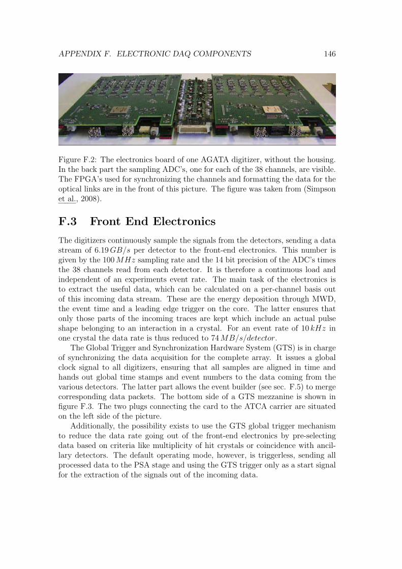
APPENDIX F. ELECTRONIC DAQ COMPONENTS 146
Figure F.2: The electronics board of one AGATA digitizer, without the housing.In the back part the sampling ADC’s, one for each of the 38 channels, are visible.The FPGA’s used for synchronizing the channels and formatting the data for theoptical links are in the front of this picture. The figure was taken from (Simpsonet al., 2008).
F.3 Front End Electronics
The digitizers continuously sample the signals from the detectors, sending a datastream of 6.19GB/s per detector to the front-end electronics. This number isgiven by the 100MHz sampling rate and the 14 bit precision of the ADC’s timesthe 38 channels read from each detector. It is therefore a continuous load andindependent of an experiments event rate. The main task of the electronics isto extract the useful data, which can be calculated on a per-channel basis outof this incoming data stream. These are the energy deposition through MWD,the event time and a leading edge trigger on the core. The latter ensures thatonly those parts of the incoming traces are kept which include an actual pulseshape belonging to an interaction in a crystal. For an event rate of 10 kHz inone crystal the data rate is thus reduced to 74MB/s/detector.
The Global Trigger and Synchronization Hardware System (GTS) is in chargeof synchronizing the data acquisition for the complete array. It issues a globalclock signal to all digitizers, ensuring that all samples are aligned in time andhands out global time stamps and event numbers to the data coming from thevarious detectors. The latter part allows the event builder (see sec. F.5) to mergecorresponding data packets. The bottom side of a GTS mezzanine is shown infigure F.3. The two plugs connecting the card to the ATCA carrier are situatedon the left side of the picture.
Additionally, the possibility exists to use the GTS global trigger mechanismto reduce the data rate going out of the front-end electronics by pre-selectingdata based on criteria like multiplicity of hit crystals or coincidence with ancil-lary detectors. The default operating mode, however, is triggerless, sending allprocessed data to the PSA stage and using the GTS trigger only as a start signalfor the extraction of the signals out of the incoming data.

APPENDIX F. ELECTRONIC DAQ COMPONENTS 147
Figure F.3: The bottom side of the GTS mezzanine card. On the left side thetwo plugs connecting the card to the ATCA carrier card can be seen.
In light of the high data rate it was decided to use ATCA1 crates for theelectronics. A mezzanine based approach was chosen for the separate tasks with
Figure F.4: An ATCA carrier cardwith all four mezzanines mounted onthe left side. The right side connectsto the back plane of the ATCA crate.
one mezzanine card each for the core, the segments and the GTS. Up to fourmezzanines can be plugged into one ATCA carrier card (see fig. F.4). It takestwo of these carriers to handle all the data from a single crystal, since one segmentmezzanine can only handle the data from six segments.
1The Advanced Telecommunications Computing Architecture is an electronics standard de-veloped for high-data rate telecommunication applications.
APPENDIX F. ELECTRONIC DAQ COMPONENTS 148
F.4 Pulse Shape Analysis
The highly challenging task of pulse shape analysis (PSA) is to disentangle theindividual γ-ray interactions within one crystal and to determine the position,the time and the energy deposition of each individual interaction by analyzingthe recorded experimental pulse shape. The output of the PSA consists only ofthe above parameters and the associated errors, allowing for the largest reductionin data rate in the whole DAQ chain. Since PSA and the related issue of pulseshape simulation are the topic of this thesis only issues relevant for the DAQ willbe covered in the following. The working principle of PSA, along with the usedalgorithms will be described in detail in chapter 4 and the reasons why a reliablesimulation is a prerequisite for a successful PSA will be given in chapter 3.
The PSA and the necessary preprocessing, outlined below, will run exclusivelyon a dedicated server farm, with one multi-processor server per crystal. Howeverthis number could change in the future, if the need arises. An important matterto note is that the PSA will be run independently for each crystal, although ascattering from one crystal to another is a likely process. But the pulse shapesare independent for each crystal since intra-detector crosstalk has been shown tobe nonexistent (Wiens, 2008). Before the traces are fed to the PSA algorithm forthe position reconstruction, some more preprocessing must be performed. Firstthe baseline must be adjusted to zero and the exponential decay originating fromthe preamplifier response functions is removed by analytic deconvolution. Beforethe traces can be normalized to unit charge in the last step, a crosstalk correction,depending on the number of hit segments, is applied.
F.5 Event Building and Merging
Each reconstructed interaction location and energy deposit keeps the timestampand event number issued by the GTS and attached to the pulse shapes. Basedon this information the event builder packs all corresponding events together andtransmits them to the tracking algorithm. At this stage the data from AGATAcan optionally be merged with time correlated data from an ancillary detector,e.g. a CD-Detector in an experiment with Coulomb excitation. Depending onthe experiment the ancillary detector may provide useful data for the trackingalgorithm in order to facilitate the determination of the emission direction of theγ-ray, important for a precise Doppler correction.

List of Figures
1.1 γ-ray spectrum of 28Ne. . . . . . . . . . . . . . . . . . . . . . . . 21.2 γ-ray spectrum of 160Dy at high spins. . . . . . . . . . . . . . . . 31.3 Schematic view of GAMMASPHERE. . . . . . . . . . . . . . . . . 61.4 Schematic drawing of the EUROBALL-III array. . . . . . . . . . . 81.5 Picture of the MINIBALL array at REX-ISOLDE, CERN. . . . . 91.6 Linear attenuation coefficients of the three main γ-ray interactions
with germanium and a sample distribution of interactions pointsfor each type. . . . . . . . . . . . . . . . . . . . . . . . . . . . . . 11
1.7 ‘World map’ view of γ-ray interaction points used in the forwardtracking algorithm. . . . . . . . . . . . . . . . . . . . . . . . . . . 12
1.8 Possible geodesic tilings of the sphere. . . . . . . . . . . . . . . . . 14
2.1 Schematic drawing of the AGATA Demonstrator. . . . . . . . . . 172.2 The AGATA longitudinal segmentation scheme, the segment la-
beling and the specifications for the encapsulation. . . . . . . . . . 192.3 AGATA angular segmentation schemes. . . . . . . . . . . . . . . . 202.4 Pictures of AGATA crystals. . . . . . . . . . . . . . . . . . . . . . 212.5 Transparent view of fully equipped asymmetric triple cluster and
without the cryostats endcap. . . . . . . . . . . . . . . . . . . . . 222.6 The AGATA Data Flow for one triple cluster . . . . . . . . . . . . 24
3.1 Geometry of the symmetric AGATA prototype. . . . . . . . . . . 303.2 The impurity concentrations as a function of depth for several
AGATA crystals, as provided by the manufacturer. . . . . . . . . 333.3 The distribution of space charge density for the S002 prototype
detector . . . . . . . . . . . . . . . . . . . . . . . . . . . . . . . . 343.4 The electric potential inside the S002 AGATA crystal. . . . . . . . 363.5 Effective segmentation of the yellow AGATA crystal. . . . . . . . 373.6 Equal energy surface for hot electrons. . . . . . . . . . . . . . . . 383.7 Anisotropy of the electron drift times. . . . . . . . . . . . . . . . . 393.8 Equal energy surface of holes near k = 0 . . . . . . . . . . . . . . 413.9 Anisotropy of hole drift times . . . . . . . . . . . . . . . . . . . . 423.10 The weighting Potential for Segment A4 at y=0 mm. . . . . . . . 44
149

LIST OF FIGURES 150
3.11 Pulse shapes for a sample interaction point . . . . . . . . . . . . . 463.12 Grid of used points depending on the interpolation order. . . . . . 473.13 Residuals from the interpolation of the core weighting potential of
a true coaxial detector as a function of the detector radius. . . . . 493.14 Precision of the interpolation routine along the outside of an AGATA
crystal. . . . . . . . . . . . . . . . . . . . . . . . . . . . . . . . . . 503.15 Residual between the simulated core signal and the inverse sum of
the simulated segment signals. . . . . . . . . . . . . . . . . . . . 523.16 The principal work flow of JASS. . . . . . . . . . . . . . . . . . . 543.17 The gain-magnitude frequency response of the preamplifier and
the anti-aliasing filter. . . . . . . . . . . . . . . . . . . . . . . . . 563.18 Response function in the time domain and effect on signal shape. 573.19 Effects of crosstalk on energy resolution and signal shape. . . . . . 593.20 Setup of the Liverpool scanning system. . . . . . . . . . . . . . . 623.21 Histogram of z-coordinates for the second tested depth. . . . . . . 653.22 Resolutions of scanning events in segment row 1 . . . . . . . . . . 673.23 Resolutions of scanning events in segment row 2. . . . . . . . . . . 683.24 Resolutions of scanning events in segment row 3. . . . . . . . . . . 693.25 Resolutions of scanning events in segment row 4. . . . . . . . . . . 703.26 Resolutions of scanning events in segment row 5. . . . . . . . . . . 713.27 Resolutions of scanning events in segment row 6. . . . . . . . . . . 723.28 Resolutions of all scanning events. . . . . . . . . . . . . . . . . . . 733.29 Comparison between scanned and simulated signals for an inter-
action in segment F1. . . . . . . . . . . . . . . . . . . . . . . . . . 763.30 Comparison of three scan signals in segment A6 with the same
nominal position close to the boundary with segment B6. Thegreat scatter in transient amplitude, especially in (b), is obviousand related to the limited precision of the scanning setup. . . . . 77
3.31 Comparison between scanned and simulated signals for an inter-action in segment A4. . . . . . . . . . . . . . . . . . . . . . . . . . 79
3.32 Illustration of the PSCS characterization technique. . . . . . . . . 803.33 Comparison between the inverse sum of the segment signals and
the core signal for the worst case. . . . . . . . . . . . . . . . . . . 813.34 Mean radial offsets in the segment rows 3 through 6. . . . . . . . 82
4.1 Dependence of the pulse shapes on the interaction location. . . . . 854.2 A sample grid of interaction locations. . . . . . . . . . . . . . . . 864.3 Sample comparison between simulated and experimental signals. . 884.4 Topology of a two-layer feedforward network . . . . . . . . . . . . 904.5 The three different activation functions . . . . . . . . . . . . . . . 934.6 Possible topologies for a particle swarm. . . . . . . . . . . . . . . 98
5.1 Power spectrum of the red crystals noise. . . . . . . . . . . . . . . 100

LIST OF FIGURES 151
5.2 Obtainable position resolution as function of t0 resolution. . . . . 1015.3 Histogram of pulse shape rise times t10 and the time between t0
and the 2σ sample. . . . . . . . . . . . . . . . . . . . . . . . . . . 1035.4 Timing resolution of the neural network for simulated data. . . . . 1045.5 All coincident events and line gated events. . . . . . . . . . . . . . 1055.6 Position resolutions for single hit events in the three front segment
rows at energies of 125 keV and 1MeV . . . . . . . . . . . . . . . 1085.7 Net charge and transient signals for two hit segments with unlike
energy split. . . . . . . . . . . . . . . . . . . . . . . . . . . . . . . 1135.8 Energy resolution in percent for double interactions in segment B1
with Eseg = 2.5MeV and its dependence on the position resolutionof the lower energetic interaction. . . . . . . . . . . . . . . . . . . 119
6.1 The setup of the test experiment. . . . . . . . . . . . . . . . . . . 1226.2 Overlay of uncorrected and Doppler-corrected spectra. . . . . . . 1246.3 Fit to Doppler-corrected peaks. . . . . . . . . . . . . . . . . . . . 1256.4 Position resolution of the energetic barycenter for single segment
hits in the simulated experimental data. The solid blue line cor-responds to the results of the FIPS algorithm and the dashed redline to the results of XGS. . . . . . . . . . . . . . . . . . . . . . . 127
E.1 Illustrations of Skewness and Kurtosis. . . . . . . . . . . . . . . . 142
F.1 Simplified schematic diagram of the AGATA preamplifiers. . . . . 144F.2 The electronics board of one AGATA digitizer. . . . . . . . . . . . 146F.3 The bottom side of the GTS mezzanine. . . . . . . . . . . . . . . 147F.4 An ATCA carrier card with all four mezzanines mounted. . . . . . 147

List of Tables
1.1 A summary of the performance of current and future detector ar-rays for a γ-ray of 1MeV and a multilpicity of Mγ = 1. . . . . . . 14
1.2 Summary of the predicted performance of AGATA for 1MeV γ-rays. 15
2.1 The specifications for the energy resolutions (FWHM) of the AGATAcrystals. For the segments the specifications define an upper limitfor each segment individually and also for the mean resolution ofall segments. . . . . . . . . . . . . . . . . . . . . . . . . . . . . . . 21
3.1 The sum of all weighting potentials interpolated at off-grid points 513.2 The position uncertainties of the scanning setup. . . . . . . . . . . 643.3 Resolutions for single event data, given in FWHM as function of
segment row. . . . . . . . . . . . . . . . . . . . . . . . . . . . . . 743.4 Median 3D distance and radial offset for each segment row. . . . . 753.5 Percentage of events resolved within ±3mm as function of segment
row. . . . . . . . . . . . . . . . . . . . . . . . . . . . . . . . . . . 75
4.1 Performance requirements of the PSA algorithm. . . . . . . . . . . 844.2 Size of the search space depending on the event type. . . . . . . . 87
5.1 Performance of the trained FNN on experimental data. The reso-lutions are quoted as FWHM of the distributions shown in figure5.5. . . . . . . . . . . . . . . . . . . . . . . . . . . . . . . . . . . . 104
5.2 Median 3D distance for single hit events at the four tested energies.1075.3 Radial Resolutions for single event data (FWHM) and percentage
of events resolved within ±3mm at the four tested energies. . . . 1095.4 Angular resolutions for single event data (FWHM) at the four
tested energies. . . . . . . . . . . . . . . . . . . . . . . . . . . . . 1095.5 Z resolutions for single event data, given in FWHM and percentage
of events resolved within ±3mm at the four tested energies. . . . 1095.6 Median 3D distance between found and correct solution for two
hit segments with equal energy. . . . . . . . . . . . . . . . . . . . 1115.7 Median 3D distance between found and correct solution for two
hit segments with unlike energy. . . . . . . . . . . . . . . . . . . . 111
152

LIST OF TABLES 153
5.8 Improvement of median 3D distance as function number of iterations.1145.9 FIPS performance for three hit segments. . . . . . . . . . . . . . . 1145.10 Median 3D distance between found and correct solution for two
hits in one segment with even energy split. . . . . . . . . . . . . . 1155.11 Median 3D distance between found and correct solution for two
hits in one segment with energy split 70%/30%. . . . . . . . . . . 1165.12 Median 3D distance between found and correct solution for two
hits in one segment with energy split 80%/20%. . . . . . . . . . . 1165.13 Median 3D distance between found and correct solution for two
hits in one segment with energy split 90%/10%. . . . . . . . . . . 1175.14 Improvement of median 3D distance as function number of itera-
tions for two hits in segment B1. . . . . . . . . . . . . . . . . . . 117
6.1 Statistics of simulated experiment. . . . . . . . . . . . . . . . . . 1236.2 Parameters of the fitted peak model, goodness of fit and resulting
FWHM of the peak for the Doppler-corrected peaks. . . . . . . . 1266.3 Position resolution of XGS and FIPS for single segment hits in the
simulated experiment. . . . . . . . . . . . . . . . . . . . . . . . . 128
A.1 Moments of X distributions . . . . . . . . . . . . . . . . . . . . . 129A.2 Moments of Y distributions. . . . . . . . . . . . . . . . . . . . . . 129A.3 Moments of Z distributions. . . . . . . . . . . . . . . . . . . . . . 130A.4 Moments of R distributions. . . . . . . . . . . . . . . . . . . . . . 130A.5 Moments of ϕ distributions. . . . . . . . . . . . . . . . . . . . . . 130
B.1 Mobility Parameters (µ in[
cm2
V s
]
) of parameter set A . . . . . . . 131
B.2 Mobility Parameters (µ in[
cm2
V s
]
) of parameter set B. . . . . . . . 132

References
Alba, E.D., & Paranjabe, V.V. 1964. Energy distribution of holes in electricfields. Phys. Lett., 11, 12–13.
Ashcroft, N.W., & Mermin, N.D. 1976. Solid State Physics. Brooks Cole.
Bazzacco, Dino. 2009. private communications.
Bishop, Christopher M. 1996. Neural Networks for Pattern Recognition. OxfordUniversity Press, USA.
Bors, Adrian G. 2000. Introduction to the Radial Basis Function Networks.http://axiom.anu.edu.au/ daa/courses/GSAC6017/rbf.pdf.
Boston, A.J., Boston, H.C., Cresswell, J.R., Dimmock, M.R., Nelson, L., Nolan,P.J., Rigby, S., Lazarus, I., Simpson, J., Medina, P., Santos, C., & Parisel,C. 2007. Gamma-ray tracking: Characterisation of the AGATA symmetricprototype detectors. Nucl. Instr. and Meth. B, 261(1-2), 1098 – 1102. Pro-ceedings of the Nineteenth International Conference on The Application ofAccelerators in Research and Industry.
Bothe, Sander. 2003. Spiking Neural Networks. Ph.D. thesis, Unversiteit Leiden.
Bronstein, I.N. 2000. Taschenbuch der Mathematik. Thun, Frankfurt am Main,Germany: Verlag Harri Deutsch.
Bruyneel, Bart. 2007. Automated optimization of detector simulation tofit S002 scan data. http://agata.lnl.infn.it/AgataWeek2007/talks/
Characterization\%20and\%20PSA/BruyneelAGATA_2007_talk2.pdf.
Bruyneel, Bart, Reiter, Peter, & Paskovici, Georghe. 2006a. Characterization oflarge volume HPGe detectors. Part I: Electron and hole mobility parameter-ization. Nucl. Instr. and Meth. A, 569, 764–773.
Bruyneel, Bart, Reiter, Peter, & Paskovici, Georghe. 2006b. Characterization oflarge volume HPGe detectors. Part II: Experimental results. Nucl. Instr. andMeth. A, 569, 774–789.
154
REFERENCES 155
Bruyneel, Bart, Reiter, Peter, Wiens, Andreas, Eberth, Jrgen, Hess, Herbert,Pascovici, Gheorghe, Warr, Nigel, & Weisshaar, Dirk. 2009. Crosstalk prop-erties of 36-fold segmented symmetric hexagonal HPGe detectors. NuclearInstruments and Methods in Physics Research Section A: Accelerators,Spectrometers, Detectors and Associated Equipment, 599(2-3), 196 – 208.
Cavalleri, G. 1971. Extension of Ramo’s theorem as applied to induced charge insemiconductor devices. Nucl. Instr. and Meth. A, 92, 137.
Clerc, M., & Kennedy, J. 2002. The particle swarm - explosion, stability, and con-vergence in a multidimensional complex space. Evolutionary Computation,IEEE Transactions on, 6(1), 58–73.
Conwell, Esther M. 1967. High Field Transport in Semiconductors. Vol. 9 ofSolid State Physics. Academic Press.
Crespi, F.C.L., Camera, F., Wieland, O., Benzoni, G., Brambilla, S., Million, B.,& Montanari, D. 2007. A pulse shape analysis algorithm for HPGe detectors.Nucl. Instr. and Meth. A, 570, 459–466.
Crespi, F.C.L., Camera, F., Million, B., Sassi, M., Wieland, O., & Bracco, A.2008. A novel technique for the characterization of a HPGe detector re-sponse based on pulse shape comparison. Nuclear Instruments and Methodsin Physics Research Section A: Accelerators, Spectrometers, Detectors andAssociated Equipment, 593(3), 440 – 447.
Deleplanque, M. A., Lee, I. Y., Vetter, K., Schmid, G. J., Stephens, F. S., Clark,R. M., Diamond, R. M., Fallon, P., & Macchiavelli, A. O. 1999. GRETA:utilizing new concepts in γ-ray detection. Nucl. Instr. and Meth. A, 430(2-3),292 – 310.
Deleplanque, M.A., & Diamond, R.M. (eds.). 1987. Gammasphere proposal.Tech. rept. LBNL-5202.
Descovich, M., Lee, I. Y., Luke, P.N., Clark, R.M., Cromaz, M., Deleplanque,M.A., Diamond, R.M., Fallon, P., Macchiavelli, A.O., Rodriguez-Vieitez,E., Stephens, F.S., & Ward, D. 2005. Effects of neutron damage on theperformance of large-volume segmented germanium detectors. Nucl. Instr.and Meth. A, 545, 199–209.
Dimmock, Matthew R. 2008. Characterisation of AGATA symmetric prototypedetectors. Ph.D. thesis, University of Liverpool.
Duchene, G., Beck, F. A., Twin, P. J., de France, G., Curien, D., Han, L.,Beausang, C. W., Bentley, M. A., Nolan, P. J., & Simpson, J. 1999. TheClover: a new generation of composite Ge detectors. Nucl. Instr. and Meth.A, 432(1), 90 – 110.
REFERENCES 156
Eberth, J., & Simpson, J. 2008. From Ge(Li) detectors to gamma-ray trackingarrays-50 years of gamma spectroscopy with germanium detectors. Prog.Part. Nucl. Phys., 60(2), 283 – 337.
Eberth, J., Brentano, P. Von, Teichert, W., Thomas, H.G., Werth, A.V.D.,Lieder, R.M., Jger, H., Kmmerling, H., Kutchin, D., Maier, K.H., Berst,M., Gutknecht, D., & Henck, R. 1992. Development of a composite Gedetector for EUROBALL. Prog. Part. Nucl. Phys., 28, 495 – 504.
Eberth, J., Thomas, H.G., Brentano, P.v., Lieder, R.M., Jger, H.M., Kmmerfing,H., Berst, M., Gutknecht, D., & Henck, R. 1996. Encapsulated Ge detectors:Development and first tests. Nucl. Instr. and Meth. A, 369(1), 135 – 140.
Eberth, J., Pascovici, G., Thomas, H. G., Warr, N., Weisshaar, D., Habs, D.,Reiter, P., Thirolf, P., Schwalm, D., Gund, C., Scheit, H., Lauer, M., Dup-pen, P. Van, Franchoo, S., Huyse, M., Lieder, R. M., Gast, W., Gerl, J., &Lieb, K. P. 2001. MINIBALL A Ge detector array for radioactive ion beamfacilities. Prog. Part. Nucl. Phys., 46(1), 389 – 398.
Eberth, Jurgen. 2008. private communications.
Essel, H.G., & Kurz, N. 2000. The general purpose data acquisition system MBS.Nuclear Science, IEEE Transactions on, 47(2), 337–339.
Fallon, P., Rodriguez-Vieitez, E., Bazin, D., Campbell, C. M., Cook, J. M.,Clark, R. M., Dinca, D-C., Gade, A., Glasmacher, T., Lee, I-Y., Macchiavelli,A. O., Mueller, W. F., Prussin, S. G., Wiedeking, M., & Yoneda, K. 2006.Transition to the Island of Inversion: Study of Excited States in 28−30Ne. J.Phys.: Conf. Ser., 49, 165–169.
Gadea, A, Marginean, N, Corradi, L, Lenzi, S M, Ur, C A, Farnea, E, de Angelis,G, Fioretto, E, Napoli, D R, Stefanini, A M, Szilner, S, Axiotis, M, Behera,B R, Latina, A, Rusu, C, Zhimin, W, Bazzacco, D, Beghini, S, Lunardi,S, Montagnoli, G, Menegazzo, R, Scarlassara, F, Vedova, F Della, Nespolo,M, Bracco, A, Camera, F, Leoni, S, Million, B, Pignanelli, M, Pollarolo, G,Trotta, M, Bizzeti, P G, Bizzeti-Sona, A M, Curien, D, Medina, P, Chambit,M, Chapman, R, Liang, X, Freeman, S J, Smith, A, Varley, B J, Pucknell,V, & Lemmon, R. 2005. The CLARA-PRISMA setup installed at LNL:first results. Journal of Physics G: Nuclear and Particle Physics, 31(10),S1443–S1448.
Gamir, L.P. 1997. A new method for the determination of the entry positionof γ-rays in HPGe detectors by current pulse analysis. Ph.D. thesis, Max-
Planck-Institut f’ur Kernphysik, Heidelberg.

REFERENCES 157
Georgiev, A., Gast, W., & Lieder, R.M. 1994. An analog-to-digital conver-sion based on a moving window deconvolution. Nuclear Science, IEEETransactions on, 41(4), 1116–1124.
Gerl, J., & Korten, W. 2001. AGATA technical proposal. Tech. rept. AGATA,http://agata.pd.infn.it/Agata-proposal.pdf.
Grave, X., Canedo, R., Clavelin, J.-F., Du, S., & Legay, E. 2005. NARVAL amodular distributed data acquisition system with Ada 95 and RTAI. RealTime Conference, 2005. 14th IEEE-NPSS, June, 5 pp.–.
Habs, D., Rudolph, D., Thirolf, P., Fischbeck, C., Gund, Ch., Schwalm, D.,Eberth, J., Grosse, E., Prade, H., Emling, H., Gerl, J., Lieder, R. M.,Duppen, P. Van, Rossi-Alvarez, C., & Pignanelli, M. 1997. Physics withGe-Miniball-arrays. Prog. Part. Nucl. Phys., 38, 111 – 126. 4 pi High Reso-lution Gamma Ray Spectroscopy and Nuclear Structure.
Hagan, Martin T., & Menhaj, Mohammad B. 1994. Training Feedforward Net-works with the Marquardt Algorithm. IEEE Trans. Neural Networks, 5,989–993.
He, Z. 2001. Review of the Shockley-Ramo theorem and its application to semi-conductor gamma-ray detectors. Nucl. Instr. and Meth. A, 463, 250–267.
Hornik, Kurt. 1991. Approximation capabilities of multilayer feedforward net-works. Neural Netw., 4(2), 251–257.
Jen, C.K. 1941. On the Induced Current and Energy Balance in Electronics.Proc. IRE, 345.
Johnson, A., Ryde, H., & Hjorth, S. A. 1972. Nuclear moment of inertia at highrotational frequencies. Nucl. Phys. A, 179(3), 753 – 768.
Kennedy, J., & Eberhart, R. 1995 (Nov/Dec). Particle swarm optimization. vol.4.
Kennedy, James, & Eberhart, Russel C. 2001. Swarm Intelligence. San Diego,USA: Morgan Kaufmann Publishers.
Kennedy, James, & Mendes, Rui. 2006. Neighborhood topologies in fully informedand best-of-neighborhood particle swarms. IEEE Trans. on Systems, Man,and Cybernetics, Part C: Applications and Reviews, 36, 515–519.
Khoo, T. L., Carpenter, M. P., Lauritsen, T., Ackermann, D., Ahmad, I., Blu-menthal, D. J., Fischer, S. M., Janssens, R. V. F., Nisius, D., Moore, E. F.,Lopez-Martens, A., Døssing, T., Krucken, R., Asztalos, S. J., Becker, J. A.,Bernstein, L., Clark, R. M., Deleplanque, M. A., Diamond, R. M., Fallon,

REFERENCES 158
P., Farris, L. P., Hannachi, F., Henry, E. A., Korichi, A., Lee, I. Y., Mac-chiavelli, A. O., & Stephens, F. S. 1996. Excitation Energies and Spins of aSuperdeformed Band in 194Hg from One-Step Discrete Decays to the YrastLine. Phys. Rev. Lett., 76(10), 1583–1586.
Knoll, Glenn F. 1999. Radiation Detection and Measurement. 3rd edn. Wiley &Sons.
Korten, W., & Lunardi, S. 2003. Achievements with the EUROBALLspectrometer 1997-2003. Tech. rept. LNL.
Kroll, Th., & Bazzacco, D. 2001. Simulation and analysis of pulse shapes fromhighly segmented HPGe detectors for the γ-ray tracking array MARS. Nucl.Instr. and Meth. A, 463(1-2), 227 – 249.
Kroll, Thorsten, & Bazzacco, Dino. 2006. A genetic algorithm for the decom-position of multiple hit events in the γ-ray tracking detector MARS. Nucl.Instr. and Meth. A, 565(2), 691 – 703.
Lazarus, I.H., Appelbe, D.E., Boston, A.J., Coleman-Smith, P.J., Cresswell, J.R.,Descovich, M., Gros, S.A.A., Lauer, M., Norman, J., Pearson, C.J., Puck-nell, V.F.E., Sampson, J.A., Turk, G., & Valiente-Dobon, J.J. 2004. TheGRT4 VME pulse processing card for segmented germanium detectors. IEEETransactions on Nuclear Science, 51(4), 1353– 1357.
Levenberg, Kenneth. 1944. A Method for the Solution of Certain Non-LinearProblems in Least Squares. The Quarterly of Applied Mathematics, 2, 164–168.
Ljungvall, Joa, & Nyberg, Johann. 2005. A study of fast neutron interactions inhigh-purity germanium detectors. Nucl. Instr. and Meth. A, 546, 553–573.
Lopez-Martens, A., Hauschild, K., Korichi, A., Roccaz, J., & Thibaud, J-P. 2004.γ-ray tracking algorithms: a comparison. Nucl. Instr. and Meth. A, 533(3),454 – 466.
Maierbeck, P., Gernhuser, R., Krcken, R., Krll, T., Alvarez-Pol, H., Aksouh,F., Aumann, T., Behr, K., Benjamim, E.A., Benlliure, J., Bildstein, V.,Bhmer, M., Boretzky, K., Borge, M.J.G., Brnle, A., Brger, A., Caamao,M., Casarejos, E., Chatillon, A., Chulkov, L.V., Cortina-Gil, D., Enders, J.,Eppinger, K., Faestermann, T., Friese, J., Fabbietti, L., Gascn, M., Geissel,H., Gerl, J., Gorska, M., Hansen, P.G., Jonson, B., Kanungo, R., Kiselev,O., Kojouharov, I., Klimkiewicz, A., Kurtukian, T., Kurz, N., Larsson, K.,Bleis, T. Le, Mahata, K., Maier, L., Nilsson, T., Nociforo, C., Nyman, G.,Pascual-Izarra, C., Perea, A., Perez, D., Prochazka, A., Rodriguez-Tajes, C.,Rossi, D., Schaffner, H., Schrieder, G., Schwertel, S., Simon, H., Sitar, B.,

REFERENCES 159
Stanoiu, M., Smmerer, K., Tengblad, O., Weick, H., Winkler, S., Brown,B.A., Otsuka, T., Tostevin, J., & Rae, W.D.M. 2009. Structure of 55Ti fromrelativistic one-neutron knockout. Physics Letters B, 675(1), 22 – 27.
Marquardt, Donald. 1963. An Algorithm for Least-Squares Estimation of Non-linear Parameters. SIAM Journal on Applied Mathematics, 11, 431–441.
Medina, P., Santos, C., & Villaume, D. 2004. A simple method for the character-ization of HPGe detectors. Instrumentation and Measurement TechnologyConference, 2004. IMTC 04. Proceedings of the 21st IEEE, 3(May), 1828–1832 Vol.3.
Medina, Patrice. 2006. private communications.
Meijering, Erik H. W., Niessen, Wiro J., Pluim, Josien P. W., & Viergever,Max A. 1999. Quantitative Comparison of Sinc-Approximating Kernels forMedical Image Interpolation. 1679 of Lecture Notes in Computer Sci-
ence.
Mendes, Rui, Kennedy, James, & Neves, Jose. 2004. The Fully Informed ParticleSwarm: Simpler, Maybe Better. IEEE Trans. on Evolutionary Computation,8, 204–210.
Mihailescu, L. 2000. Principles and methods for γ-ray tracking with large volumegermanium detectors. Ph.D. thesis, Universitat Bonn.
Mihailescu, L., Gast, Werner, Lieder, R. M., Brands, H., & Jager, H. 2000. Theinfluence of anisotropic electron drift velocity on the signal shapes of closed-end HPGe detectors. Nucl. Instr. and Meth. A, 447, 350–360.
Minsky, M.L., & Papert, S. A. 1969. Perceptrons: An Introduction toComputational Geometry. MIT Press.
Monaghan, J.J. 1985. Particle Methods for Hydrodynamics. Computer PhysicsReports, 3, 71–124.
Montana, David J., & Davis, Lawrence. 1989. Training Feedforward Neural Net-works Using Genetic Algorithms. Pages 762–767 of: IJCAI.
NASA. 2006. Intelligent Flight Control System.http://www.nasa.gov/centers/dryden/news/FactSheets/FS-076-DFRC.html.
Nathan, Marshall I. 1963. Anisotropy of the Conductivity of n-Type Germaniumat High Electric Fields. Phys. Rev., 130(6), 2201–2204.
REFERENCES 160
Nguyen, Derrick, & Widrow, Bernard. 1990. Improving the Learning Speed of 2-Layer Neural Networks by Choosing Initial Values of the Adaptive Weights.Pages 21–26 of: Proceedings of the International Joint Conference on NeuralNetworks, vol. 3. IEEE.
Olariu, A., Desesquelles, P., Diarra, Ch., Medina, P., Parisel, C., & Collaboration,C.S.Obot.A. 2006. Pulse shape analysis for the location of the γ-interactionsin AGATA. Nuclear Science, IEEE Transactions on, 53(3), 1028–1031.
Ottaviani, G., Reggiani, L., Canali, C., Nava, F., & Quaranta, A. Alberigi. 1975.Hole drift velocity in silicon. Phys. Rev. B, 12, 3318.
Pinson, W.E., & Bray, R. 1964. Experimental determination of the energy distri-bution functions and analysis of the energy-loss mechanisms of hot carriersin p-type germanium. Phys. Rev., 136, 1449–1466.
Radford, David C. 2005. private communications.
Ramo, S. 1939. Currents induced by electron motion. Proc. IRE 27, 584.
Recchia, F., Bazzacco, D., Farnea, E., Gadea, A., Venturelli, R., Beck, T., Bed-narczyk, P., Buerger, A., Dewald, A., Dimmock, M., Duchne, G., Eberth,J., Faul, T., Gerl, J., Gernhaeuser, R., Hauschild, K., Holler, A., Jones,P., Korten, W., Krll, Th., Krcken, R., Kurz, N., Ljungvall, J., Lunardi, S.,Maierbeck, P., Mengoni, D., Nyberg, J., Nelson, L., Pascovici, G., Reiter,P., Schaffner, H., Schlarb, M., Steinhardt, T., Thelen, O., Ur, C.A., Dobon,J.J. Valiente, & Weihaar, D. 2009. Position resolution of the prototypeAGATA triple-cluster detector from an in-beam experiment. Nucl. Instr.and Meth. A, 604(3), 555 – 562.
Reggiani, L., Canali, C., Nava, F., & Ottaviani, G. 1977. Hole drift velocity ingermanium. Phys. Rev. B, 16, 2781–2791.
Reggiani, L., Canali, C., Nava, F., Pozhela, Y.K., Asche, M., Komiyama, S.,Kurosawa, T., Masumi, T., Hess, K., Iafrate, G.J., & Constant, E. 1985.Hot-Electron Transport in Semiconductors. Vol. 58 of Topics in AppliedPhysics. Springer-Verlag.
Reik, H. G., & Risken, H. 1962. Drift Velocity and Anisotropy of Hot Electronsin n Germanium. Phys. Rev., 126(5), 1737–1746.
Reynolds, Craig W. 1987. Flocks, Herds, and Schools: A Distributed BehavioralModel. Computer Graphics, 21(4), 25–34.
Rosenblatt, Frank. 1958. The Perceptron: A Probabilistic Model for InformationStorage and Organization in the Brain. Psychological Review, 65, 386–408.

REFERENCES 161
Rummelhart, D.E., Hinton, G.E., & Williams, R.J. 1986. Learning internalrepresentations by error propagation. Vol. 1. The M.I.T. Press. Pages318–362.
Sasaki, W., & Shibuya, M. 1956. Experimental evidence of the anisotropy of hotelectrons in n-type germanium. J. Phys. Soc. Jpn., 11, 1202–1203.
Schmid, G. J., Deleplanque, M. A., Lee, I. Y., Stephens, F. S., Vetter, K., Clark,R. M., Diamond, R. M., Fallon, P., Macchiavelli, A. O., & MacLeod, R. W.1999. A γ-ray tracking algorithm for the GRETA spectrometer. Nucl. Instr.and Meth. A, 430(1), 69 – 83.
Schmid, G.J., Lee, I.Y., Deleplanque, M.A., Hendriks, P., Stephens, F.S., Vetter,K., Asztalos, S.J., Clark, R.M., Diamond, R.M., Fallon, P., Kruecken, R.,Macchiavelli, A.O., & MacLeod, R.W. 1997. Gamma-ray cluster identifica-tion in a spherical shell of highly segmented germanium detectors. NuclearScience, IEEE Transactions on, 44(3), 975–978.
Schonberg, Isaac J. 1946. Contributions to the problem of approximation ofequidistant data by analytic functions, Part A: On the problem of smoothingor graduation, a first class of analytic approximation formulas. Quart. Appl.Math., 4, 45–99.
Shannon, Claude E. 1949. Communication in the presence of noise. Proceedingsof the Institute of Radio Engineers, 37(1), 10–21.
Shockley, W. 1938. Currents on Conductors Induced by a Moving Point Charge.J. Appl. Phys., 9, 635–636.
Simpson, J., Korten, W., & Nyberg, J. 2008. AGATA Technical Design Report.Tech. rept. AGATA.
Trottenberg, U., Oosterlee., C.W., & Schuller, A. 2000. Multigrid. AcademicPress.
Unsworth, Carl. 2009. private communications.
van der Marel, J., & Cederwall, B. 1999. Backtracking as a way to reconstructCompton scattered γ-rays. Nucl. Instr. and Meth. A, 437(2-3), 538 – 551.
Vetter, K., Kuhn, A., Lee, I. Y., Clark, R. M., Cromaz, M., Deleplanque, M. A.,Diamond, R. M., Fallon, P., Lane, G. J., Macchiavelli, A. O., Maier, M. R.,Stephens, F. S., Svensson, C. E., & Yaver, H. 2000a. Performance of theGRETA prototype detectors. Nucl. Instr. and Meth. A, 452(1-2), 105 – 114.

REFERENCES 162
Vetter, K., Kuhn, A., Deleplanque, M. A., Lee, I. Y., Stephens, F. S., Schmid,G. J., Beckedahl, D., Blair, J. J., Clark, R. M., Cromaz, M., Diamond, R. M.,Fallon, P., Lane, G. J., Kammeraad, J. E., Macchiavelli, A. O., & Svensson,C. E. 2000b. Three-dimensional position sensitivity in two-dimensionallysegmented HP-Ge detectors. Nucl. Instr. and Meth. A, 452(1-2), 223 – 238.
Wiens, Andreas. 2008. CAT of AGATA detectors & The AGATA triple clusterdetector. http://www.agata.org/aw7/presentations.
Wilson, Edward O. 2000. Sociobiology: The New Synthesis. Harvard UniversityPress.
Zocca, F., Pullia, A., Boiano, C., & Bassini, R. 2007. A Smart Reset Circuit forLow-Noise Preamplifiers of X- ? Ray Sensor Signals. IEEE Trans. Nucl. Sci.,54(1), 197–201.

Danksagung
Als erstes mochte ich Prof. Dr. Reiner Krucken fur die Moglichkeit zu einer sehrinteressanten Doktorarbeit und die immer vorhandene herzliche Unterstutzungdanken. Roman Gernhauser verdient besonderen Dank nicht nur fur die intensiveBetreuung sondern auch fur anregende Diskussionen und entsprechende Denk-anstoße.
Eine so Computer-lastige Arbeit wie diese erfordert naturlich einen reibungs-losen Betrieb der Rechenfarm. Ohne die fleißige Arbeit der Admins, insbesondereLudwig Maier, ware dies schlicht unmoglich. Im Anschluss bedanke ich michgleich noch bei meinen Kollegen die sehr verstandnisvoll waren wenn die Farmmal wieder komplett von mir belegt war. Ralf, Sigrid (Danke fur die Zeitun-gen!), Michael und Wolfgang danke ich fur die angenehmen Mittagspausen undGesprache, auch wenn die Bayern am Tag zuvor mal wieder schlecht gespielthatten. Die angenehme Arbeitsatmosphare bei uns im Buro weiß ich sehr zuschatzen. Des weiteren danke ich den Mitgliedern der AGATA Kollaboration furihren Beitrag zum Gelingen dieser Arbeit. Ich mochte mich noch bei Freundenund Verwandtschaft fur das Verstandnis bedanken wenn ich mal keine Zeit hatte.
Naturlich verdient auch meine Familie gebuhrend Dank. Konni, Dennis undMelissa, ihr ward sehr geduldig mit mir und habt es immer wieder geschafft mirdie Ablenkung und Erholung zu bieten, die bisweilen ziemlich notwendig war.Konni, ich kann dir nicht genugend dafur danken wie positiv du mein Lebenverandert hast und wirst. Schließlich gebuhrt meinen Eltern ein großes Dan-keschon. Ihr habt mir nicht nur das Studium und die Doktorarbeit ermoglichtsondern mich auch immer nach besten Kraften unterstutzt.
163


![[Paper introduction] Performance Capture of Interacting Characters with Handheld Kinects](https://static.fdocument.pub/doc/165x107/55a6844b1a28ab2b498b47c1/paper-introduction-performance-capture-of-interacting-characters-with-handheld-kinects.jpg)