SimpleMKL - Idiap Research Institute

Journal of Machine Learning Research X (2008) 1-34 Submitted 01/08; Revised 08/08; Published XX/XX

SimpleMKL

Alain Rakotomamonjy [email protected] EA 4108Universite de Rouen76800 Saint Etienne du Rouvray, France

Francis R. Bach [email protected] - WILLOW Project - TeamLaboratoire d’Informatique de l’Ecole Normale Superieure(CNRS/ENS/INRIA UMR 8548)45, Rue d’Ulm, 75230 Paris, France

Stephane Canu [email protected] EA 4108INSA de Rouen76801 Saint Etienne du Rouvray, France

Yves Grandvalet [email protected]

Idiap Research Institute, Centre du Parc, 1920 Martigny, SwitzerlandHeudiasyc, CNRS/Universite de Technologie de Compiegne (UMR 6599), 60205 Compiegne, France

Editor: Nello Cristianini

Abstract

Multiple kernel learning (MKL) aims at simultaneously learning a kernel and the associ-ated predictor in supervised learning settings. For the support vector machine, an efficientand general multiple kernel learning algorithm, based on semi-infinite linear progamming,has been recently proposed. This approach has opened new perspectives since it makesMKL tractable for large-scale problems, by iteratively using existing support vector ma-chine code. However, it turns out that this iterative algorithm needs numerous iterationsfor converging towards a reasonable solution. In this paper, we address the MKL prob-lem through a weighted 2-norm regularization formulation with an additional constrainton the weights that encourages sparse kernel combinations. Apart from learning the com-bination, we solve a standard SVM optimization problem, where the kernel is defined asa linear combination of multiple kernels. We propose an algorithm, named SimpleMKL,for solving this MKL problem and provide a new insight on MKL algorithms based onmixed-norm regularization by showing that the two approaches are equivalent. We showhow SimpleMKL can be applied beyond binary classification, for problems like regression,clustering (one-class classification) or multiclass classification. Experimental results showthat the proposed algorithm converges rapidly and that its efficiency compares favorablyto other MKL algorithms. Finally, we illustrate the usefulness of MKL for some regres-sors based on wavelet kernels and on some model selection problems related to multiclassclassification problems.

c©2008 Rakotomamonjy et al..

Rakotomamonjy et al.

1. Introduction

During the last few years, kernel methods, such as support vector machines (SVM) haveproved to be efficient tools for solving learning problems like classification or regression(Scholkopf and Smola, 2001). For such tasks, the performance of the learning algorithmstrongly depends on the data representation. In kernel methods, the data representationis implicitly chosen through the so-called kernel K(x, x′). This kernel actually plays tworoles: it defines the similarity between two examples x and x′, while defining an appropriateregularization term for the learning problem.

Let {xi, yi}`i=1 be the learning set, where xi belongs to some input space X and yi is thetarget value for pattern xi. For kernel algorithms, the solution of the learning problem isof the form

f(x) =∑

i=1

α?iK(x, xi) + b?, (1)

where α?i and b? are some coefficients to be learned from examples, while K(·, ·) is a given

positive definite kernel associated with a reproducing kernel Hilbert space (RKHS) H.In some situations, a machine learning practitioner may be interested in more flexible

models. Recent applications have shown that using multiple kernels instead of a singleone can enhance the interpretability of the decision function and improve performances(Lanckriet et al., 2004a). In such cases, a convenient approach is to consider that the kernelK(x, x′) is actually a convex combination of basis kernels:

K(x, x′) =M∑

m=1

dmKm(x, x′) , with dm ≥ 0 ,M∑

m=1

dm = 1 ,

where M is the total number of kernels. Each basis kernel Km may either use the full set ofvariables describing x or subsets of variables stemming from different data sources (Lanck-riet et al., 2004a). Alternatively, the kernels Km can simply be classical kernels (such asGaussian kernels) with different parameters. Within this framework, the problem of datarepresentation through the kernel is then transferred to the choice of weights dm.

Learning both the coefficients αi and the weights dm in a single optimization problem isknown as the multiple kernel learning (MKL) problem. For binary classification, the MKLproblem has been introduced by Lanckriet et al. (2004b), resulting in a quadratically con-strained quadratic programming problem that becomes rapidly intractable as the numberof learning examples or kernels become large.

What makes this problem difficult is that it is actually a convex but non-smooth min-imization problem. Indeed, Bach et al. (2004a) have shown that the MKL formulation ofLanckriet et al. (2004b) is actually the dual of a SVM problem in which the weight vectorhas been regularized according to a mixed (`2, `1)-norm instead of the classical squared`2-norm. Bach et al. (2004a) have considered a smoothed version of the problem for whichthey proposed a SMO-like algorithm that enables to tackle medium-scale problems.

Sonnenburg et al. (2006) reformulate the MKL problem of Lanckriet et al. (2004b) asa semi-infinite linear program (SILP). The advantage of the latter formulation is that thealgorithm addresses the problem by iteratively solving a classical SVM problem with a singlekernel, for which many efficient toolboxes exist (Vishwanathan et al., 2003; Loosli et al.,

2

SimpleMKL

2005; Chang and Lin, 2001), and a linear program whose number of constraints increasesalong with iterations. A very nice feature of this algorithm is that is can be extended toa large class of convex loss functions. For instance, Zien and Ong (2007) have proposed amulticlass MKL algorithm based on similar ideas.

In this paper, we present another formulation of the multiple learning problem. We firstdepart from the primal formulation proposed by Bach et al. (2004a) and further used byBach et al. (2004b) and Sonnenburg et al. (2006). Indeed, we replace the mixed-norm regu-larization by a weighted `2-norm regularization, where the sparsity of the linear combinationof kernels is controlled by a `1-norm constraint on the kernel weights. This new formula-tion of MKL leads to a smooth and convex optimization problem. By using a variationalformulation of the mixed-norm regularization, we show that our formulation is equivalentto the ones of Lanckriet et al. (2004b), Bach et al. (2004a) and Sonnenburg et al. (2006).

The main contribution of this paper is to propose an efficient algorithm, named Sim-pleMKL, for solving the MKL problem, through a primal formulation involving a weighted`2-norm regularization. Indeed, our algorithm is simple, essentially based on a gradientdescent on the SVM objective value. We iteratively determine the combination of kernelsby a gradient descent wrapping a standard SVM solver, which is SimpleSVM in our case.Our scheme is similar to the one of Sonnenburg et al. (2006), and both algorithms minimizethe same objective function. However, they differ in that we use reduced gradient descent inthe primal, whereas Sonnenburg et al.’s SILP relies on cutting planes. We will empiricallyshow that our optimization strategy is more efficient, with new evidences confirming thepreliminary results reported in Rakotomamonjy et al. (2007).

Then, extensions of SimpleMKL to other supervised learning problems such as regressionSVM, one-class SVM or multiclass SVM problems based on pairwise coupling are proposed.Although it is not the main purpose of the paper, we will also discuss the applicability ofour approach to general convex loss functions.

This paper also presents several illustrations of the usefulness of our algorithm. Forinstance, in addition to the empirical efficiency comparison, we also show, in a SVM regres-sion problem involving wavelet kernels, that automatic learning of the kernels leads to farbetter performances. Then we depict how our MKL algorithm behaves on some multiclassproblems.

The paper is organized as follows. Section 2 presents the functional settings of our MKLproblem and its formulation. Details on the algorithm and discussion of convergence andcomputational complexity are given in Section 3. Extensions of our algorithm to otherSVM problems are discussed in Section 4 while experimental results dealing with computa-tional complexity or with comparison with other model selection methods are presented inSection 5.

A SimpleMKL toolbox based on Matlab code is available at http://www.mloss.org.This toolbox is an extension of our SVM-KM toolbox (Canu et al., 2003).

2. Multiple Kernel Learning Framework

In this section, we present our MKL formulation and derive its dual. In the sequel, iand j are indices on examples, wheras m is the kernel index. In order to lighten notations,

3


we omit to specify that summations on i and j go from 1 to `, and that summations on mgo from 1 to M .

2.1 Functional framework

Before entering into the details of the MKL optimization problem, we first present thefunctional framework adopted for multiple kernel learning. Assume Km,m = 1, ...,M areM positive definite kernels on the same input space X , each of them being associated withan RKHS Hm endowed with an inner product 〈·, ·〉m. For any m, let dm be a non-negativecoefficient and H′m be the Hilbert space derived from Hm as follows:

H′m = {f | f ∈ Hm :‖f‖Hm

dm<∞} ,

endowed with the inner product

〈f, g〉H′m =1dm〈f, g〉m .

In this paper, we use the convention that x0 = 0 if x = 0 and ∞ otherwise. This means

that, if dm = 0 then a function f belongs to the Hilbert space H′m only if f = 0 ∈ Hm. Insuch a case, H′m is restricted to the null element of Hm.

Within this framework, H′m is a RKHS with kernel K(x, x′) = dm Km(x, x′) since

∀f ∈ H′m ⊆ Hm , f(x) = 〈f(·),Km(x, ·)〉m=

1dm〈f(·), dmKm(x, ·)〉m

= 〈f(·), dmKm(x, ·)〉H′m .

Now, if we define H as the direct sum of the spaces H′m, i.e.,

H =M⊕

m=1

H′m ,

then, a classical result on RKHS (Aronszajn, 1950) says that H is a RKHS of kernel

K(x, x′) =M∑

m=1

dmKm(x, x′) .

Owing to this simple construction, we have built a RKHS H for which any function is asum of functions belonging to Hm. In our framework, MKL aims at determining the set ofcoefficients {dm} within the learning process of the decision function. The multiple kernellearning problem can thus be envisioned as learning a predictor belonging to an adaptivehypothesis space endowed with an adaptive inner product. The forthcoming sections explainhow we solve this problem.

4

SimpleMKL

2.2 Multiple kernel learning primal problem

In the SVM methodology, the decision function is of the form given in equation (1),where the optimal parameters α?

i and b? are obtained by solving the dual of the followingoptimization problem:

minf,b,ξ

12‖f‖2H + C

∑

i

ξi

s.t. yi(f(xi) + b) ≥ 1− ξi ∀iξi ≥ 0 ∀i .

In the MKL framework, one looks for a decision function of the form f(x) + b =∑m fm(x) + b, where each function fm belongs to a different RKHS Hm associated with

a kernel Km. According to the above functional framework and inspired by the multiplesmoothing splines framework of Wahba (1990, chap. 10), we propose to address the MKLSVM problem by solving the following convex problem (see proof in appendix), which wewill be referred to as the primal MKL problem:

min{fm},b,ξ,d

12

∑m

1dm‖fm‖2Hm

+ C∑

i

ξi

s.t. yi

∑m

fm(xi) + yib ≥ 1− ξi ∀iξi ≥ 0 ∀i∑m

dm = 1 , dm ≥ 0 ∀m ,

(2)

where each dm controls the squared norm of fm in the objective function.The smaller dm is, the smoother fm (as measured by ‖fm‖Hm) should be. When dm = 0,

‖fm‖Hm has also to be equal to zero to yield a finite objective value. The `1-norm constrainton the vector d is a sparsity constraint that will force some dm to be zero, thus encouragingsparse basis kernel expansions.

2.3 Connections with mixed-norm regularization formulation of MKL

The MKL formulation introduced by Bach et al. (2004a) and further developed by Son-nenburg et al. (2006) consists in solving an optimization problem expressed in a functionalform as

min{f},b,ξ

12

(∑m

‖fm‖Hm

)2

+ C∑

i

ξi

s.t. yi

∑m

fm(xi) + yib ≥ 1− ξi ∀iξi ≥ 0 ∀i.

(3)

Note that the objective function of this problem is not smooth since ‖fm‖Hm is not differen-tiable at fm = 0. However, what makes this formulation interesting is that the mixed-normpenalization of f =

∑m fm is a soft-thresholding penalizer that leads to a sparse solution,

for which the algorithm performs kernel selection (Bach, 2008). We have stated in theprevious section that our problem should also lead to sparse solutions. In the following, weshow that the formulations (2) and (3) are equivalent.

5


For this purpose, we simply show that the variational formulation of the mixed-normregularization is equal to the weighted 2-norm regularization, (which is a particular case of amore general equivalence proposed by Micchelli and Pontil (2005)) i.e., by Cauchy-Schwartzinequality, for any vector d on the simplex:

(∑m

‖fm‖Hm

)2

=

(∑m

‖fm‖Hm

d1/2m

d1/2m

)2

6(∑

m

‖fm‖2Hm

dm

)(∑m

dm

)

6∑m

‖fm‖2Hm

dm,

where equality is met when d1/2m is proportional to ‖fm‖Hm/d

1/2m , that is:

dm =‖fm‖Hm∑q

‖fq‖Hq

, (4)

which leads to

mindm≥0,

Pm dm=1

∑m

‖fm‖2Hm

dm=

(∑m

‖fm‖Hm

)2

. (5)

Hence, owing to this variational formulation, the non-smooth mixed-norm objectivefunction of problem (3) has been turned into a smooth objective function in problem (2).Although the number of variables has increased, we will see that this problem can be solvedmore efficiently.

2.4 The MKL dual problem

The dual problem is a key point for deriving MKL algorithms and for studying theirconvergence properties. Since our primal problem (2) is equivalent to the one of Bach et al.(2004a), they lead to the same dual. However, our primal formulation being convex anddifferentiable, it provides a simple derivation of the dual, that does not use conic duality.

The Lagrangian of problem (2) is

L =12

∑m

1dm‖fm‖2Hm

+ C∑

i

ξi +∑

i

αi

(1− ξi − yi

∑m

fm(xi)− yib

)−

∑

i

νiξi

+λ

(∑m

dm − 1

)−

∑m

ηmdm , (6)

where αi and νi are the Lagrange multipliers of the constraints related to the usual SVMproblem, whereas λ and ηm are associated to the constraints on dm. When setting to zero

6

SimpleMKL

the gradient of the Lagrangian with respect to the primal variables, we get the following

(a)1dm

fm(·) =∑

i

αiyiKm(·, xi) , ∀m

(b)∑

i

αiyi = 0

(c) C − αi − νi = 0 , ∀i(d) − 1

2‖fm‖2Hm

d2m

+ λ− ηm = 0 , ∀m .

(7)

We note again here that fm(·) has to go to 0 if the coefficient dm vanishes. Plugging theseoptimality conditions in the Lagrangian gives the dual problem

maxαi,λ

∑

i

αi − λ

s.t.∑

i

αiyi = 0

0 ≤ αi ≤ C ∀i12

∑

i,j

αiαjyiyjKm(xi, xj) ≤ λ , ∀m .

(8)

This dual problem1 is difficult to optimize due to the last constraint. This constraintmay be moved to the objective function, but then, the latter becomes non-differentiablecausing new difficulties (Bach et al., 2004a). Hence, in the forthcoming section, we proposean approach based on the minimization of the primal. In this framework, we benefit fromdifferentiability which allows for an efficient derivation of an approximate primal solution,whose accuracy will be monitored by the duality gap.

3. Algorithm for solving the MKL primal problem

One possible approach for solving problem (2) is to use the alternate optimization algo-rithm applied by Grandvalet and Canu (1999, 2003) in another context. In the first step,problem (2) is optimized with respect to fm, b and ξ, with d fixed. Then, in the secondstep, the weight vector d is updated to decrease the objective function of problem (2), withfm, b and ξ being fixed. In Section 2.3, we showed that the second step can be carried outin closed form. However, this approach lacks convergence guarantees and may lead to nu-merical problems, in particular when some elements of d approach zero (Grandvalet, 1998).Note that these numerical problems can be handled by introducing a perturbed version ofthe alternate algorithm as shown by Argyriou et al. (2008).

Instead of using an alternate optimization algorithm, we prefer to consider here thefollowing constrained optimization problem:

mindJ(d) such that

M∑

m=1

dm = 1, dm ≥ 0 , (9)

1. Note that Bach et al. (2004a) formulation differs slightly, in that the kernels are weighted by somepre-defined coefficients that were not considered here.

7


where

J(d) =

min{f},b,ξ

12

∑m

1dm‖fm‖2Hm

+ C∑

i

ξi ∀i

s.t. yi

∑m

fm(xi) + yib ≥ 1− ξiξi ≥ 0 ∀i .

(10)

We show below how to solve problem (9) on the simplex by a simple gradient method. Wewill first note that the objective function J(d) is actually an optimal SVM objective value.We will then discuss the existence and computation of the gradient of J(·), which is at thecore of the proposed approach.

3.1 Computing the optimal SVM value and its derivatives

The Lagrangian of problem (10) is identical to the first line of equation (6). By setting tozero the derivatives of this Lagrangian according to the primal variables, we get conditions(7) (a) to (c), from which we derive the associated dual problem

maxα

−12

∑

i,j

αiαjyiyj

∑m

dmKm(xi, xj) +∑

i

αi

with∑

i

αiyi = 0

C ≥ αi ≥ 0 ∀i ,

(11)

which is identified as the standard SVM dual formulation using the combined kernelK(xi, xj) =

∑m dmKm(xi, xj). Function J(d) is defined as the optimal objective value

of problem (10). Because of strong duality, J(d) is also the objective value of the dualproblem:

J(d) = −12

∑

i,j

α?iα

?jyiyj

∑m

dmKm(xi, xj) +∑

i

α?i , (12)

where α? maximizes (11). Note that the objective value J(d) can be obtained by any SVMalgorithm. Our method can thus take advantage of any progress in single kernel algorithms.In particular, if the SVM algorithm we use is able to handle large-scale problems, so willour MKL algorithm. Thus, the overall complexity of SimpleMKL is tied to the one of thesingle kernel SVM algorithm.

From now on, we assume that each Gram matrix (Km(xi, xj))i,j is positive definite,with all eigenvalues greater than some η > 0 (to enforce this property, a small ridge maybe added to the diagonal of the Gram matrices). This implies that, for any admissiblevalue of d, the dual problem is strictly concave with convexity parameter η (Lemarechaland Sagastizabal, 1997). In turn, this strict concavity property ensures that α? is unique,a characteristic that eases the analysis of the differentiability of J(·).

Existence and computation of derivatives of optimal value functions such as J(·) havebeen largely discussed in the literature. For our purpose, the appropriate reference isTheorem 4.1 in Bonnans and Shapiro (1998), which has already been applied by Chapelleet al. (2002) for tuning squared-hinge loss SVM. This theorem is reproduced in the appendixfor self-containedness. In a nutshell, it says that differentiability of J(d) is ensured by

8

SimpleMKL

the unicity of α?, and by the differentiability of the objective function that gives J(d).Furthermore, the derivatives of J(d) can be computed as if α? were not to depend on d.Thus, by simple differentiation of the dual function (11) with respect to dm, we have:

∂J

∂dm= −1

2

∑

i,j

α?iα

?jyiyjKm(xi, xj) ∀m . (13)

We will see in the sequel that the applicability of this theorem can be extended to otherSVM problems. Note that complexity of the gradient computation is of the order of m ·n2

SV ,with nSV being the number of support vectors for the current d.

3.2 Reduced gradient algorithm

The optimization problem we have to deal with in (9) is a non-linear objective functionwith constraints over the simplex. With our positivity assumption on the kernel matrices,J(·) is convex and differentiable with Lipschitz gradient (Lemarechal and Sagastizabal,1997). The approach we use for solving this problem is a reduced gradient method, whichconverges for such functions (Luenberger, 1984).

Once the gradient of J(d) is computed, d is updated by using a descent direction ensuringthat the equality constraint and the non-negativity constraints on d are satisfied. Wehandle the equality constraint by computing the reduced gradient (Luenberger, 1984, Chap.11). Let dµ be a non-zero entry of d, the reduced gradient of J(d), denoted ∇redJ , hascomponents:

[∇redJ ]m =∂J

∂dm− ∂J

∂dµ∀m 6= µ , and [∇redJ ]µ =

∑

m6=µ

(∂J

∂dµ− ∂J

∂dm

).

We chose µ to be the index of the largest component of vector d, for better numericalstability (Bonnans, 2006).

The positivity constraints have also to be taken into account in the descent direction.Since we want to minimize J(·), −∇redJ is a descent direction. However, if there is an indexm such that dm = 0 and [∇redJ ]m > 0, using this direction would violate the positivityconstraint for dm. Hence, the descent direction for that component is set to 0. This givesthe descent direction for updating d as

Dm =

0 if dm = 0 and ∂J∂dm− ∂J

∂dµ> 0

− ∂J

∂dm+∂J

∂dµif dm > 0 and m 6= µ

∑

g 6=µ,dν>0

(∂J

∂dν− ∂J

∂dµ

)for m = µ .

(14)

The usual updating scheme is d← d+γD , where γ is the step size. Here, as detailed inAlgorithm 1, we go one step beyond: once a descent direction D has been computed, we firstlook for the maximal admissible step size in that direction and check whether the objectivevalue decreases or not. The maximal admissible step size corresponds to a component, saydν , set to zero. If the objective value decreases, d is updated, we setDν = 0 and normalizeDto comply with the equality constraint. This procedure is repeated until the objective value

9


Algorithm 1 SimpleMKL algorithmset dm = 1

M for m = 1, . . . ,Mwhile stopping criterion not met do

compute J(d) by using an SVM solver with K =∑

m dmKm

compute ∂J∂dm

for m = 1, . . . ,M and descent direction D (14).set µ = argmax

mdm, J† = 0, d† = d, D† = D

while J† < J(d) do {descent direction update}d = d†, D = D†

ν = argmin{m|Dm<0}

−dm/Dm, γmax = −dν/Dν

d† = d+ γmaxD, D†µ = Dµ −Dν , D

†ν = 0

compute J† by using an SVM solver with K =∑

m d†mKm

end whileline search along D for γ ∈ [0, γmax] {calls an SVM solver for each γ trial value}d← d+ γD

end while

stops decreasing. At this point, we look for the optimal step size γ, which is determined byusing a one-dimensional line search, with proper stopping criterion, such as Armijo’s rule,to ensure global convergence.

In this algorithm, computing the descent direction and the line search are based on theevaluation of the objective function J(·), which requires solving an SVM problem. Thismay seem very costly but, for small variations of d, learning is very fast when the SVMsolver is initialized with the previous values of α? (DeCoste and Wagstaff., 2000). Notethat the gradient of the cost function is not computed after each update of the weightvector d. Instead, we take advantage of an easily updated descent direction as long as theobjective value decreases. We will see in the numerical experiments that this approachsaves a substantial amount of computation time compared to the usual update schemewhere the descent direction is recomputed after each update of d. Note that we have alsoinvestigated gradient projection algorithms (Bertsekas, 1999, Chap 2.3), but this turned outto be slightly less efficient than the proposed approach, and we will not report these results.

The algorithm is terminated when a stopping criterion is met. This stopping criterioncan be either based on the duality gap, the KKT conditions, the variation of d betweentwo consecutive steps or, even more simply, on a maximal number of iterations. Ourimplementation, based on the duality gap, is detailed in the forthcoming section.

3.3 Optimality conditions

In a convex constrained optimization algorithm such as the one we are considering, wehave the opportunity to check for proper optimality conditions such as the KKT conditionsor the duality gap (the difference between primal and dual objective values), which shouldbe zero at the optimum. From the primal and dual objectives provided respectively in (2)and (8), the MKL duality gap is

10

SimpleMKL

DualGap = J(d?)−∑

i

α?i +

12

maxm

∑

i,j

α?iα

?jyiyjKm(xi, xj) , ,

where d? and {α?i } are optimal primal and dual variables, and J(d?) depends implicitly on

optimal primal variables {f?m}, b? and {ξ?

i }. If J(d?) has been obtained through the dualproblem (11), then this MKL duality gap can also be computed from the single kernel SVMalgorithm duality gap DGSVM. Indeed, equation (12) holds only when the single kernelSVM algorithm returns an exact solution with DGSVM = 0. Otherwise, we have

DGSVM = J(d?) +12

∑

i,j

α?iα

?jyiyj

∑m

d?mKm(xi, xj)−

∑

i

α?i

then the MKL duality gap becomes

DualGap = DGSVM − 12

∑

i,j

α?iα

?jyiyj

∑m

d?mKm(xi, xj) +

12

maxm

∑

i,j

α?iα

?jyiyjKm(xi, xj) .

Hence, it can be obtained with a small additional computational cost compared to the SVMduality gap.

In iterative procedures, it is common to stop the algorithm when the optimality condi-tions are respected up to a tolerance threshold ε. Obviously, SimpleMKL has no impact onDGSVM, hence, one may assume, as we did here, that DGSVM needs not to be monitored.Consequently, we terminate the algorithm when

maxm

∑

i,j

α?iα

?jyiyjKm(xi, xj)−

∑

i,j

α?iα

?jyiyj

∑m

d?mKm(xi, xj) ≤ ε . (15)

For some of the other MKL algorithms that will be presented in Section 4, the dualfunction may be more difficult to derive. Hence, it may be easier to rely on approximateKKT conditions as a stopping criterion. For the general MKL problem (9), the first orderoptimality conditions are obtained through the KKT conditions:

∂J

∂dm+ λ− ηm = 0 ∀mηm · dm = 0 ∀m ,

where λ and {ηm} are respectively the Lagrange multipliers for the equality and inequalityconstraints of (9). These KKT conditions imply

∂J

∂dm= −λ if dm > 0

∂J

∂dm≥ −λ if dm = 0 .

However, as Algorithm 1 is not based on the Lagrangian formulation of problem (9), λis not computed. Hence, we derive approximate necessary optimality conditions to be usedfor termination criterion. Let’s define dJmin and dJmax as

dJmin = min{dm|dm>0}

∂J

∂dmand dJmax = max

{dm|dm>0}∂J

∂dm,

11


then, the necessary optimality conditions are approximated by the following terminationconditions:

|dJmin − dJmax| ≤ ε and∂J

∂dm≥ dJmax if dm = 0

In other words, we are considered at the optimum when the gradient components for allpositive dm lie in a ε-tube and when all gradient components for vanishing dm are outsidethis tube. Note that these approximate necessary optimality conditions are available rightaway for any differentiable objective function J(d).

3.4 Cutting Planes, Steepest Descent and Computational Complexity

As we stated in the introduction, several algorithms have been proposed for solving theoriginal MKL problem defined by Lanckriet et al. (2004b). All these algorithms are basedon equivalent formulations of the same dual problem; they all aim at providing a pair ofoptimal vectors (d, α).

In this subsection, we contrast SimpleMKL with its closest relative, the SILP algorithmof Sonnenburg et al. (2005, 2006). Indeed, from an implementation point of view, thetwo algorithms are alike, since they are wrapping a standard single kernel SVM algorithm.This feature makes both algorithms very easy to implement. They, however, differ incomputational efficiency, because the kernel weights dm are optimized in quite differentways, as detailed below.

Let us first recall that our differentiable function J(d) is defined as:

J(d) =

maxα

−12

∑

i,j

αiαjyiyj

∑m

dmKm(xi, xj) +∑

i

αi

with∑

i

αiyi = 0, C ≥ αi ≥ 0 ∀i ,

and both algorithms aim at minimizing this differentiable function. However, using a SILPapproach in this case, does not take advantage of the smoothness of the objective function.

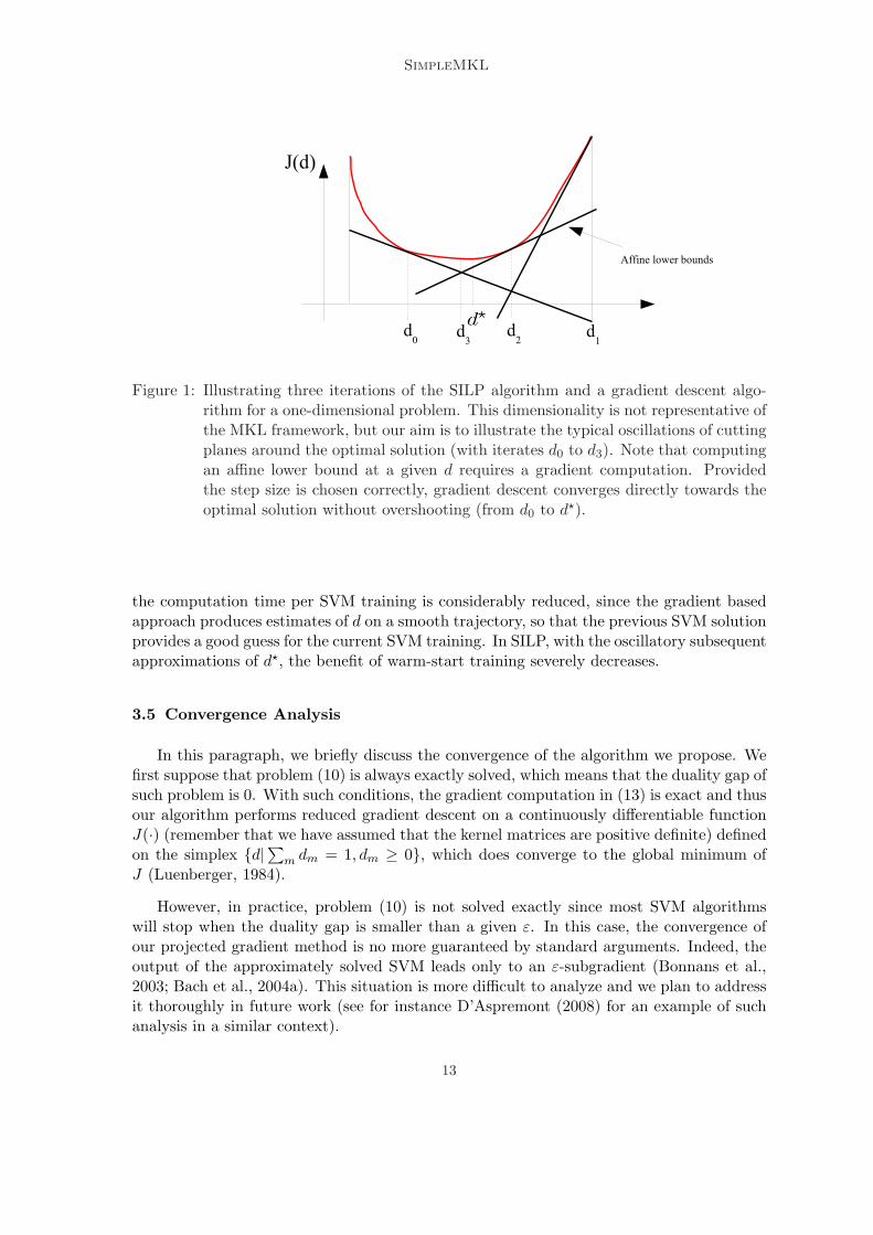
The SILP algorithm of Sonnenburg et al. (2006) is a cutting plane method to minimize Jwith respect to d. For each value of d, the best α is found and leads to an affine lower boundon J(d). The number of lower bounding affine functions increases as more (d, α) pairs arecomputed, and the next candidate vector d is the minimizer of the current lower bound onJ(d), that is, the maximum over all the affine functions. Cutting planes method do convergebut they are known for their instability, notably when the number of lower-bounding affinefunctions is small: the approximation of the objective function is then loose and the iteratesmay oscillate (Bonnans et al., 2003). Our steepest descent approach, with the proposed linesearch, does not suffer from instability since we have a differentiable function to minimize.Figure 1 illustrates the behaviour of both algorithms in a simple case, with oscillations forcutting planes and direct convergence for gradient descent.

Section 5 evaluates how these oscillations impact on the computational time of theSILP algorithm on several examples. These experiments show that our algorithm needsless costly gradient computations. Conversely, the line search in the gradient base approachrequires more SVM retrainings in the process of querying the objective function. However,

12

SimpleMKL

Figure 1: Illustrating three iterations of the SILP algorithm and a gradient descent algo-rithm for a one-dimensional problem. This dimensionality is not representative ofthe MKL framework, but our aim is to illustrate the typical oscillations of cuttingplanes around the optimal solution (with iterates d0 to d3). Note that computingan affine lower bound at a given d requires a gradient computation. Providedthe step size is chosen correctly, gradient descent converges directly towards theoptimal solution without overshooting (from d0 to d?).

the computation time per SVM training is considerably reduced, since the gradient basedapproach produces estimates of d on a smooth trajectory, so that the previous SVM solutionprovides a good guess for the current SVM training. In SILP, with the oscillatory subsequentapproximations of d?, the benefit of warm-start training severely decreases.

3.5 Convergence Analysis

In this paragraph, we briefly discuss the convergence of the algorithm we propose. Wefirst suppose that problem (10) is always exactly solved, which means that the duality gap ofsuch problem is 0. With such conditions, the gradient computation in (13) is exact and thusour algorithm performs reduced gradient descent on a continuously differentiable functionJ(·) (remember that we have assumed that the kernel matrices are positive definite) definedon the simplex {d|∑m dm = 1, dm ≥ 0}, which does converge to the global minimum ofJ (Luenberger, 1984).

However, in practice, problem (10) is not solved exactly since most SVM algorithmswill stop when the duality gap is smaller than a given ε. In this case, the convergence ofour projected gradient method is no more guaranteed by standard arguments. Indeed, theoutput of the approximately solved SVM leads only to an ε-subgradient (Bonnans et al.,2003; Bach et al., 2004a). This situation is more difficult to analyze and we plan to addressit thoroughly in future work (see for instance D’Aspremont (2008) for an example of suchanalysis in a similar context).

13


4. Extensions

In this section, we discuss how the proposed algorithm can be simply extended to otherSVM algorithms such as SVM regression, one-class SVM or pairwise multiclass SVM algo-rithms. More generally, we will discuss other loss functions that can be used within ourMKL algorithms.

4.1 Extensions to other SVM Algorithms

The algorithm we described in the previous section focuses on binary classificationSVMs, but it is worth noting that our MKL algorithm can be extended to other SVMalgorithms with only little changes. For SVM regression with the ε-insensitive loss, or clus-tering with the one-class soft margin loss, the problem only changes in the definition of theobjective function J(d) in (10).

For SVM regression (Vapnik et al., 1997; Scholkopf and Smola, 2001), we have

J(d) =

minfm,b,ξi

12

∑m

1dm‖fm‖2Hm

+ C∑

i

(ξi + ξ∗i )

s.t. yi −∑m

fm(xi)− b ≤ ε+ ξi ∀i∑m

fm(xi) + b− yi ≤ ε+ ξ∗i ∀iξi ≥ 0, ξ∗i ≤ 0 ∀i ,

(16)

and for one-class SVMs (Scholkopf and Smola, 2001), we have:

J(d) =

minfm,b,ξi

12

∑m

1dm‖fm‖2Hm

+1ν`

∑

i

ξi − b

s.t.∑m

fm(xi) ≥ b− ξiξi ≥ 0 .

(17)

Again, J(d) can be defined according to the dual functions of these two optimization prob-lems, which are respectively

J(d) =

maxα,β

∑

i

(βi − αi)yi − ε∑

i

(βi + αi)− 12

∑

i,j

(βi − αi)(βj − αj)∑m

dmKm(xi, xj)

with∑

i

(βi − αi) = 0

0 ≤ αi , βi ≤ C, ∀i ,(18)

and

J(d) =

maxα

−12

∑

i,j

αiαj

∑m

dmKm(xi, xj)

with 0 ≤ αi ≤ 1ν`

∀i∑

i

αi = 1 ,

(19)

14

SimpleMKL

where {αi} and {βi} are Lagrange multipliers.Then, as long as J(d) is differentiable, a property strictly related to the strict concavityof its dual function, our descent algorithm can still be applied. The main effort for theextension of our algorithm is the evaluation of J(d) and the computation of its derivatives.Like for binary classification SVM, J(d) can be computed by means of efficient off-the-shelfSVM solvers and the gradient of J(d) is easily obtained through the dual problems. ForSVM regression, we have:

∂J

∂dm= −1

2

∑

i,j

(β?i − α?

i )(β?j − α?

j )Km(xi, xj) ∀m , (20)

and for one-class SVM, we have:

∂J

∂dm= −1

2

∑

i,j

α?iα

?jKm(xi, xj) ∀m , (21)

where α?i and β?

i are the optimal values of the Lagrange multipliers. These examplesillustrate that extending SimpleMKL to other SVM problems is rather straighforward. Thisobservation is valid for other SVM algorithms (based for instance on the ν parameter, asquared hinge loss or squared-ε tube) that we do not detail here. Again, our algorithmcan be used provided J(d) is differentiable, by plugging in the algorithm the function thatevaluates the objective value J(d) and its gradient. Of course, the duality gap may beconsidered as a stopping criterion if it can be computed.

4.2 Multiclass Multiple Kernel Learning

With SVMs, multiclass problems are customarily solved by combining several binaryclassifiers. The well-known one-against-all and one-against-one approaches are the twomost common ways for building a multiclass decision function based on pairwise decisionfunctions. Multiclass SVM may also be defined right away as the solution of a globaloptimization problem (Weston and Watkins, 1999; Crammer and Singer, 2001), that mayalso be addressed with structured-output SVM (Tsochantaridis et al., 2005). Very recently,an MKL algorithm based on structured-output SVM has been proposed by Zien and Ong(2007). This work extends the work of Sonnenburg et al. (2006) to multiclass problems,with an MKL implementation still based on a QCQP or SILP approach.

Several works have compared the performance of multiclass SVM algorithms (Duan andKeerthi, 2005; Hsu and Lin, 2002; Rifkin and Klautau, 2004). In this subsection, we donot deal with this aspect; we explain how SimpleMKL can be extended to pairwise SVMmulticlass implementations. The problem of applying our algorithm to structured-outputSVM will be briefly discussed later.

Suppose we have a multiclass problem with P classes. For a one-against-all multiclassSVM, we need to train P binary SVM classifiers, where the p-th classifier is trained by con-sidering all examples of class p as positive examples while all other examples are considerednegative. For a one-against-one multiclass problem, P (P − 1)/2 binary SVM classifiers arebuilt from all pairs of distinct classes. Our multiclass MKL extension of SimpleMKL differsfrom the binary version only in the definition of a new cost function J(d). As we now look

15


for the combination of kernels that jointly optimizes all the pairwise decision functions, theobjective function we want to optimize according to the kernel weights {dm} is:

J(d) =∑

p∈PJp(d) ,

where P is the set of all pairs to be considered, and Jp(d) is the binary SVM objective valuefor the classification problem pertaining to pair p.

Once the new objective function is defined, the lines of Algorithm 1 still apply. Thegradient of J(d) is still very simple to obtain, since owing to linearity, we have:

∂J

∂dm= −1

2

∑

p∈P

∑

i,j

α?i,pα

?j,pyiyjKm(xi, xj) ∀m , (22)

where αj,p is the Lagrange multiplier of the j-th example involved in the p-th decisionfunction. Note that those Lagrange multipliers can be obtained independently for eachpair.

The approach described above aims at finding the combination of kernels that jointlyoptimizes all binary classification problems: this one set of features should maximize thesum of margins. Another possible and straightforward approach consists in running inde-pendently SimpleMKL for each classification task. However, this choice is likely to resultin as many combinations of kernels as there are binary classifiers.

4.3 Other loss functions

Multiple kernel learning has been of great interest and since the seminal work of Lanck-riet et al. (2004b), several works on this topic have flourished. For instance, multiple kernellearning has been transposed to least-square fitting and logistic regression (Bach et al.,2004b). Independently, several authors have applied mixed-norm regularization, such asthe additive spline regression model of Grandvalet and Canu (1999). This type of regular-ization, which is now known as the group lasso, may be seen as a linear version of multiplekernel learning (Bach, 2008). Several algorithms have been proposed for solving the grouplasso problem. Some of them are based on projected gradient or on coordinate descentalgorithm. However, they all consider the non-smooth version of the problem.

We previously mentioned that Zien and Ong (2007) have proposed an MKL algorithmbased on structured-output SVMs. For such problem, the loss function, which differs fromthe usual SVM hinge loss, leads to an algorithm based on cutting planes instead of theusual QP approach.

Provided the gradient of the objective value can be obtained, our algorithm can beapplied to group lasso and structured-output SVMs. The key point is whether the theoremof Bonnans et al. (2003) can be applied or not. Although we have not deeply investigatedthis point, we think that many problems comply with this requirement, but we leave thesedevelopments for future work.

4.4 Approximate regularization path

SimpleMKL requires the setting of the usual SVM hyperparameter C, which usuallyneeds to be tuned for the problem at hand. For doing so, a practical and useful technique

16

SimpleMKL

is to compute the so-called regularization path, which describes the set of solutions as Cvaries from 0 to ∞.

Exact path following techniques have been derived for some specific problems like SVMsor the lasso (Hastie et al., 2004; Efron et al., 2004). Besides, regularization paths can besampled by predictor-corrector methods (Rosset, 2004; Bach et al., 2004b).

For model selection purposes, an approximation of the regularization path may be suf-ficient. This approach has been applied for instance by Koh et al. (2007) in regularizedlogistic regression.

Here, we compute an approximate regularization path based on a warm-start technique.Suppose, that for a given value of C, we have computed the optimal (d?, α?) pair; the ideaof a warm-start is to use this solution for initializing another MKL problem with a differentvalue of C. In our case, we iteratively compute the solutions for decreasing values of C(note that α? has to be modified to be a feasible initialization of the more constrained SVMproblem).

5. Numerical experiments

In this experimental section, we essentially aim at illustrating three points. The firstpoint is to show that our gradient descent algorithm is efficient. This is achieved by binaryclassification experiments, where SimpleMKL is compared to the SILP approach of Sonnen-burg et al. (2006). Then, we illustrate the usefulness of a multiple kernel learning approachin the context of regression. The examples we use are based on wavelet-based regression inwhich the multiple kernel learning framework naturally fits. The final experiment aims atevaluating the multiple kernel approach in a model selection problem for some multiclassproblems.

5.1 Computation time

The aim of this first set of experiments is to assess the running times of SimpleMKL. 2

First, we compare with SILP regarding the time required for computing a single solutionof MKL with a given C hyperparameter. Then, we compute an approximate regularizationpath by varying C values. We finally provide hints on the expected complexity of Sim-pleMKL, by measuring the growth of running time as the number of examples or kernelsincreases.

5.1.1 Time needed for reaching a single solution

In this first benchmark, we put SimpleMKL and SILP side by side, for a fixed valueof the hyperparameter C (C = 100). This procedure, which does not take into account aproper model selection procedure, is not representative of the typical use of SVMs. It ishowever relevant for the purpose of comparing algorithmic issues.

The evaluation is made on five datasets from the UCI repository: Liver, Wpbc, Iono-sphere, Pima, Sonar (Blake and Merz, 1998). The candidate kernels are:

2. All the experiments have been run on a Pentium D-3 GHz with 3 GB of RAM.

17


• Gaussian kernels with 10 different bandwidths σ, on all variables and on each singlevariable;

• polynomial kernels of degree 1 to 3, again on all and each single variable.

All kernel matrices have been normalized to unit trace, and are precomputed prior torunning the algorithms.

Both SimpleMKL and SILP wrap an SVM dual solver based on SimpleSVM, an activeconstraints method written in Matlab (Canu et al., 2003). The descent procedure of Sim-pleMKL is also implemented in Matlab, whereas the linear programming involved in SILPis implemented in the publicly available toolbox LPSOLVE (Berkelaar et al., 2004).

For a fair comparison, we use the same stopping criterion for both algorithms. Theyhalt when, either the duality gap is lower than 0.01, or the number of iterations exceeds2000. Quantitatively, the displayed results differ from the preliminary version of this work,where the stopping criterion was based on the stabilization of the weights, but they arequalitatively similar (Rakotomamonjy et al., 2007).

For each dataset, the algorithms were run 20 times with different train and test sets(70% of the examples for training and 30% for testing). Training examples were normalizedto zero mean and unit variance.

In Table 1, we report different performance measures: accuracy, number of selectedkernels and running time. As the latter is mainly spent in querying the SVM solver and incomputing the gradient of J with respect to d, the number of calls to these two routines isalso reported.

Both algorithms are nearly identical in performance accuracy. Their number of selectedkernels are of same magnitude, although SimpleMKL tends to select 10 to 20% more ker-nels. As both algorithms address the same convex optimization problem, with convergentmethods starting from the same initialization, the observed differences are only due to theinaccuracy of the solution when the stopping criterion is met. Hence, the trajectories chosenby each algorithm for reaching the solution, detailed in Section 3.4, explain the differencesin the number of selected kernels. The updates of dm based on the descent algorithm ofSimpleMKL are rather conservative (small steps departing from 1/M for all dm), whereasthe oscillations of cutting planes are likely to favor extreme solutions, hitting the edges ofthe simplex.

This explanation is corroborated by Figure 2, which compares the behavior of the dm

coefficients through time. The instability of SILP is clearly visible, with very high oscilla-tions in the first iterations and a noticeable residual noise in the long run. In comparison,the trajectories for SimpleSVM are much smoother.

If we now look at the overall difference in computation time reported in Table 1, clearly,on all data sets, SimpleSVM is faster than SILP, with an average gain factor of about 5.Furthermore, the larger the number of kernels is, the larger the speed gain we achieve.Looking at the last column of Table 1, we see that the main reason for improvement is thatSimpleMKL converges in fewer iterations (that is, gradient computations). It may seemsurprising that this gain is not conterbalanced by the fact that SimpleMKL requires manymore calls to the SVM solver (on average, about 4 times). As we stated in Section 3.4,when the number of kernels is large, computing the gradient may be expensive comparedto SVM retraining with warm-start techniques.

18

SimpleMKL

Table 1: Average performance measures for the two MKL algorithms and a plain gradientdescent algorithm.

Liver ` = 241 M = 91Algorithm # Kernel Accuracy Time (s) # SVM eval # Gradient evalSILP 10.6 ± 1.3 65.9 ± 2.6 47.6 ± 9.8 99.8 ± 20 99.8 ± 20SimpleMKL 11.2 ± 1.2 65.9 ± 2.3 18.9 ± 12.6 522 ± 382 37.0 ± 26Grad. Desc. 11.6 ± 1.3 66.1 ± 2.7 31.3 ± 14.2 972 ± 630 103 ± 27

Pima ` = 538 M = 117Algorithm # Kernel Accuracy Time (s) # SVM eval # Gradient evalSILP 11.6 ± 1.0 76.5 ± 2.3 224 ± 37 95.6 ± 13 95.6 ± 13SimpleMKL 14.7 ± 1.4 76.5 ± 2.6 79.0 ± 13 314 ± 44 24.3 ± 4.8Grad. Desc. 14.8 ± 1.4 75.5 ± 2.5 219 ± 24 873 ± 147 118 ± 8.7

Ionosphere ` = 246 M = 442Algorithm # Kernel Accuracy Time (s) # SVM eval # Gradient evalSILP 21.6 ± 2.2 91.7 ± 2.5 535 ± 105 403 ± 53 403 ± 53SimpleMKL 23.6 ± 2.6 91.5 ± 2.5 123 ± 46 1170 ± 369 64 ± 25Grad. Desc. 22.9 ± 3.2 92.1 ± 2.5 421 ± 61.9 4000 ± 874 478 ± 38

Wpbc ` = 136 M = 442Algorithm # Kernel Accuracy Time (s) # SVM eval # Gradient evalSILP 13.7 ± 2.5 76.8 ± 1.2 88.6 ± 32 157 ± 44 157 ± 44SimpleMKL 15.8 ± 2.4 76.7 ± 1.2 20.6 ± 6.2 618 ± 148 24 ± 10Grad. Desc. 16.8 ± 2.8 76.9 ± 1.5 106 ± 6.1 2620 ± 232 361 ± 16

Sonar ` = 146 M = 793Algorithm # Kernel Accuracy Time (s) # SVM eval # Gradient evalSILP 33.5 ± 3.8 80.5 ± 5.1 2290± 864 903 ± 187 903 ± 187SimpleMKL 36.7 ± 5.1 80.6 ± 5.1 163 ± 93 2770 ± 1560 115 ± 66Grad. Desc. 35.7 ± 3.9 80.2 ± 4.7 469 ± 90 7630 ± 2600 836 ± 99

19


0 2 4 6 8 10 120

0.1

0.2

0.3

0.4d k S

impl

eMK

L

0 20 40 60 80 100 1200

0.1

0.2

0.3

0.4

Iterations

d k SIL

P

0 10 20 30 40 50 60 700

0.1

0.2

0.3

0.4

d k Sim

pleM

KL

0 50 100 150 200 250 300 3500

0.1

0.2

0.3

0.4

Iterations

d k SIL

P

Pima Ionosphere

Figure 2: Evolution of the five largest weights dm for SimpleMKL and SILP; left row: Pima;right row: Ionosphere.

To understand why, with this large number of calls to the SVM solver, SimpleMKL isstill much faster than SILP, we have to look back at Figure 2. On the one hand, the largevariations in subsequents dm values for SILP, entail that subsequent SVM problems are notlikely to have similar solutions: a warm-start call to the SVM solver does not help much.On the other hand, with the smooth trajectories of dm in SimpleMKL, the previous SVMsolution is often a good guess for the current problem: a warm-start call to the SVM solverresults in much less computation than a call from scratch.

Table 1 also shows the results obtained when replacing the update scheme describedin Algorithm 1 by a usual reduced gradient update, which, at each iteration, modifies dby computing the optimal step size on the descent direction D (14). The training of thisvariant is considerably slower than SimpleMKL and is only slightly better than SILP. Wesee that the gradient descent updates require many more calls to the SVM solver and anumber of gradient computations comparable with SILP. Note that, compared to SILP, thenumerous additional calls to the SVM solver have not a drastic effect on running time. Thegradient updates are stable, so that they can benefit from warm-start contrary to SILP.

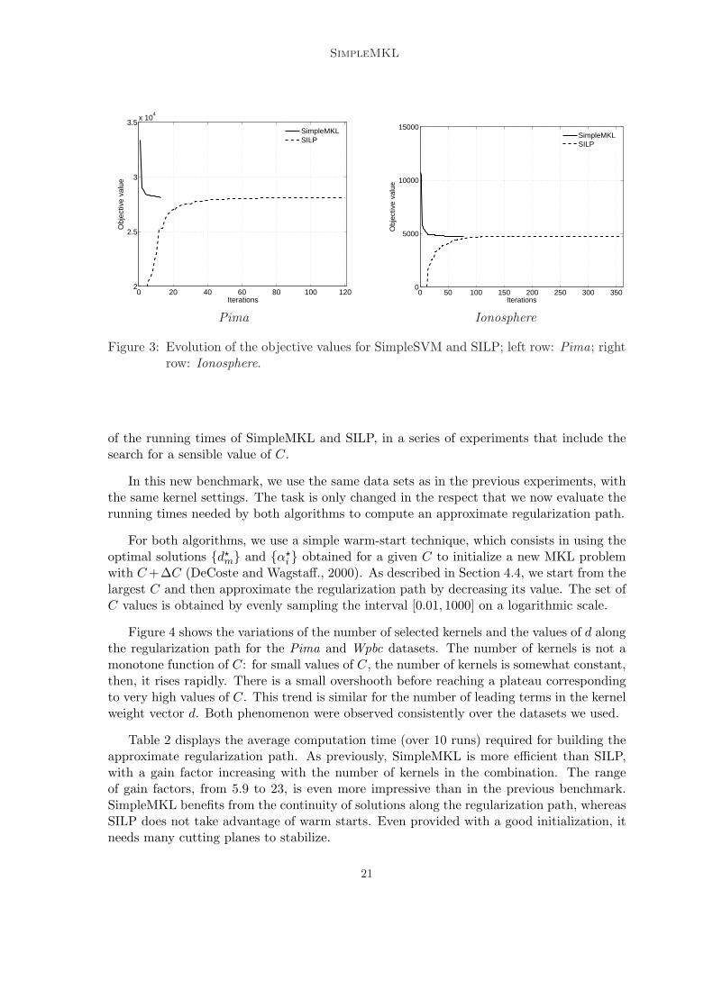
To end this first series of experiments, Figure 3 depicts the evolution of the objectivefunction for the data sets that were used in Figure 2. Besides the fact that SILP needs moreiterations for achieving a good approximation of the final solution, it is worth noting thatthe objective values rapidly reach their steady state while still being far from convergence,when dm values are far from being settled. Thus, monitoring objective values is not suitableto assess convergence.

5.1.2 Time needed for getting an approximate regularization path

In practice, the optimal value of C is unknown, and one has to solve several SVM prob-lems, spanning a wide range of C values, before choosing a solution according to some modelselection criterion like the cross-validation error. Here, we further pursue the comparison

20

SimpleMKL

0 20 40 60 80 100 1202

2.5

3

3.5x 10

4O

bjec

tive

valu

e

Iterations

SimpleMKLSILP

0 50 100 150 200 250 300 3500

5000

10000

15000

Obj

ectiv

e va

lue

Iterations

SimpleMKLSILP

Pima Ionosphere

Figure 3: Evolution of the objective values for SimpleSVM and SILP; left row: Pima; rightrow: Ionosphere.

of the running times of SimpleMKL and SILP, in a series of experiments that include thesearch for a sensible value of C.

In this new benchmark, we use the same data sets as in the previous experiments, withthe same kernel settings. The task is only changed in the respect that we now evaluate therunning times needed by both algorithms to compute an approximate regularization path.

For both algorithms, we use a simple warm-start technique, which consists in using theoptimal solutions {d?

m} and {α?i } obtained for a given C to initialize a new MKL problem

with C+∆C (DeCoste and Wagstaff., 2000). As described in Section 4.4, we start from thelargest C and then approximate the regularization path by decreasing its value. The set ofC values is obtained by evenly sampling the interval [0.01, 1000] on a logarithmic scale.

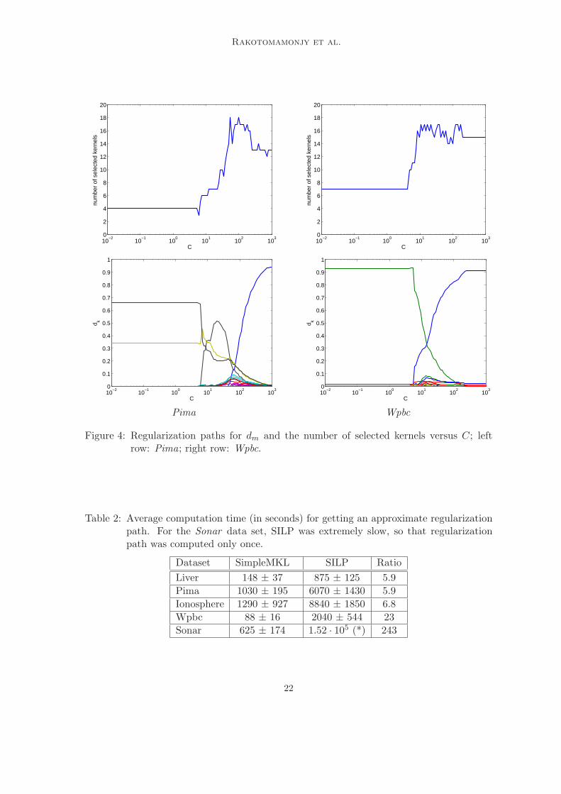
Figure 4 shows the variations of the number of selected kernels and the values of d alongthe regularization path for the Pima and Wpbc datasets. The number of kernels is not amonotone function of C: for small values of C, the number of kernels is somewhat constant,then, it rises rapidly. There is a small overshooth before reaching a plateau correspondingto very high values of C. This trend is similar for the number of leading terms in the kernelweight vector d. Both phenomenon were observed consistently over the datasets we used.

Table 2 displays the average computation time (over 10 runs) required for building theapproximate regularization path. As previously, SimpleMKL is more efficient than SILP,with a gain factor increasing with the number of kernels in the combination. The rangeof gain factors, from 5.9 to 23, is even more impressive than in the previous benchmark.SimpleMKL benefits from the continuity of solutions along the regularization path, whereasSILP does not take advantage of warm starts. Even provided with a good initialization, itneeds many cutting planes to stabilize.

21


10−2

10−1

100

101

102

103

0

2

4

6

8

10

12

14

16

18

20

C

num

ber

of s

elec

ted

kern

els

10−2

10−1

100

101

102

103

0

2

4

6

8

10

12

14

16

18

20

C

num

ber

of s

elec

ted

kern

els

10−2

10−1

100

101

102

103

0

0.1

0.2

0.3

0.4

0.5

0.6

0.7

0.8

0.9

1

C

d k

10−2

10−1

100

101

102

103

0

0.1

0.2

0.3

0.4

0.5

0.6

0.7

0.8

0.9

1

C

d k

Pima Wpbc

Figure 4: Regularization paths for dm and the number of selected kernels versus C; leftrow: Pima; right row: Wpbc.

Table 2: Average computation time (in seconds) for getting an approximate regularizationpath. For the Sonar data set, SILP was extremely slow, so that regularizationpath was computed only once.

Dataset SimpleMKL SILP RatioLiver 148 ± 37 875 ± 125 5.9Pima 1030 ± 195 6070 ± 1430 5.9Ionosphere 1290 ± 927 8840 ± 1850 6.8Wpbc 88 ± 16 2040 ± 544 23Sonar 625 ± 174 1.52 · 105 (*) 243

22

SimpleMKL

5.1.3 More on SimpleMKL running times

Here, we provide an empirical assessment of the expected complexity of SimpleMKLon different data sets from the UCI repository. We first look at the situation where kernelmatrices can be pre-computed and stored in memory, before reporting experiments wherethe memory are too high, leading to repeated kernel evaluations.

In a first set of experiments, we use Gaussian kernels, computed on random subsets ofvariables and with random width. These kernels are precomputed and stored in memory,and we report the average CPU running times obtained from 20 runs differing in the randomdraw of training examples. The stopping criterion is the same as in the previous section: arelative duality gap less than ε = 0.01.

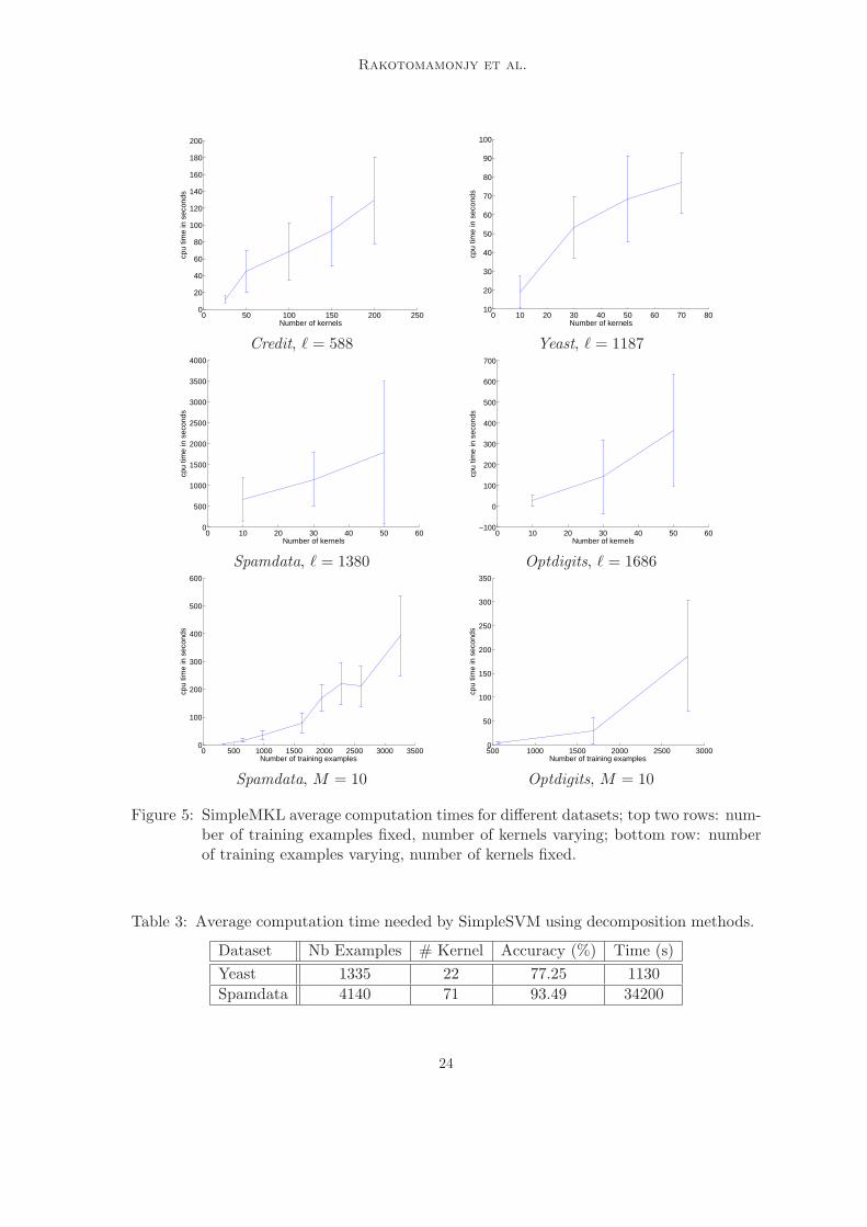
The first two rows of Figure 5 depicts the growth of computation time as the num-ber of kernel increases. We observe a nearly linear trend for the four learning problems.This growth rate could be expected considering the linear convergence property of gradienttechniques, but the absence of overhead is valuable.

The last row of Figure 5 depicts the growth of computation time as the number ofexamples increases. Here, the number of kernels is set to 10. In these plots, the observedtrend is clearly superlinear. Again, this trend could be expected, considering that SVMexpected training times are superlinear in the number of training examples. As we alreadymentioned, the complexity of SimpleMKL is tightly linked to the one of SVM training (forsome examples of single kernel SVM running time, one can refer to the work of Loosli andCanu (2007)).

When all the kernels used for MKL cannot be stored in memory, one can resort to adecomposition method. Table 3 reports the average computation times, over 10 runs, in thismore difficult situation. The large-scale SVM scheme of Joachims (1999) has been imple-mented, with basis kernels recomputed whenever needed. This approach is computationallyexpensive but goes with no memory limit. For these experiments, the stopping criterion isbased on the variation of the weights dm. As shown in Figure 2, the kernel weights rapidlyreach a steady state and many iterations are spent for fine tuning the weight and reach theduality gap tolerance. Here, we trade the optimality guarantees provided by the dualitygap for substantial computational time savings. The algorithm terminates when the kernelweights variation is lower than 0.001.

Results reported in Table 3 just aim at showing that medium and large-scale situationscan be handled by SimpleMKL. Note that Sonnenburg et al. (2006) have run a modifiedversion of their SILP algorithm on a larger scale datasets. However, for such experiments,they have taken advantage of some specific feature map properties. And, as they stated,for general cases where kernel matrices are dense, they have to rely on the SILP algorithmwe used in this section for efficiency comparison .

5.2 Multiple kernel regression examples

Several research papers have already claimed that using multiple kernel learning canlead to better generalization performances in some classification problems (Lanckriet et al.,2004a; Zien and Ong, 2007; Harchaoui and Bach, 2007). This next experiment aims atillustrating this point but in the context of regression. The problem we deal with is aclassical univariate regression problem where the design points are irregular (D’Amato et al.,

23


0 50 100 150 200 2500

20

40

60

80

100

120

140

160

180

200

Number of kernels

cpu

time

in s

econ

ds

0 10 20 30 40 50 60 70 8010

20

30

40

50

60

70

80

90

100

Number of kernels

cpu

time

in s

econ

ds

Credit, ` = 588 Yeast, ` = 1187

0 10 20 30 40 50 600

500

1000

1500

2000

2500

3000

3500

4000

Number of kernels

cpu

time

in s

econ

ds

0 10 20 30 40 50 60−100

0

100

200

300

400

500

600

700

Number of kernels

cpu

time

in s

econ

ds

Spamdata, ` = 1380 Optdigits, ` = 1686

0 500 1000 1500 2000 2500 3000 35000

100

200

300

400

500

600

Number of training examples

cpu

time

in s

econ

ds

500 1000 1500 2000 2500 30000

50

100

150

200

250

300

350

Number of training examples

cpu

time

in s

econ

ds

Spamdata, M = 10 Optdigits, M = 10

Figure 5: SimpleMKL average computation times for different datasets; top two rows: num-ber of training examples fixed, number of kernels varying; bottom row: numberof training examples varying, number of kernels fixed.

Table 3: Average computation time needed by SimpleSVM using decomposition methods.

Dataset Nb Examples # Kernel Accuracy (%) Time (s)Yeast 1335 22 77.25 1130Spamdata 4140 71 93.49 34200

24

SimpleMKL

2006). Furthermore, according to equation (16), we look for the regression function f(x)as a linear combination of functions each belonging to a wavelet based reproducing kernelHilbert space.

The algorithm we use is a classical SVM regression algorithm with multiple kernels whereeach kernel is built from a set of wavelets. These kernels have been obtained according tothe expression:

K(x, x′) =∑

j

∑s

12jψj,s(x)ψj,s(x′)

where ψ(·) is a mother wavelet and j,s are respectively the dilation and translation pa-rameters of the wavelet ψj,s(·). The theoretical details on how such kernels can been builtare available in D’Amato et al. (2006); Rakotomamonjy and Canu (2005); Rakotomamonjyet al. (2005).

Our hope when using multiple kernel learning in this context is to capture the multiscalestructure of the target function. Hence, each kernel involved in the combination should beweighted accordingly to its correlation to the target function. Furthermore, such a kernelhas to be built according to the multiscale structure we wish to capture. In this experiment,we have used three different choices of multiple kernels setting. Suppose we have a set ofwavelets with j ∈ [jmin, jmax] and s ∈∈ [smin, smax].

First of all, we have build a single kernel from all the wavelets according to the aboveequation. Then we have created kernels from all wavelets of a given scale (dilation)

KDil,J(x, x′) =smax∑

s=smin

12jψJ,s(x)ψJ,s(x′) ∀J ∈ [jmin, jmax]

and lastly, we have a set of kernels, where each kernel is built from wavelets located at agiven scale and given time-location:

KDil−Trans,J,S(x, x′) =∑

s=S

12jψJ,s(x)ψJ,s(x′) ∀J ∈ [jmin, jmax]

where S is a given set of translation parameter. These sets are built by splitting the fulltranslation parameters index in contiguous and non-overlapping index. The mother waveletwe used is a Symmlet Daubechies wavelet with 6 vanishing moments. The resolution levelsof the wavelet goes from jmin = −3 to jmin = 6. According to these settings, we have 10dilation kernels and 48 dilation-translation kernels.

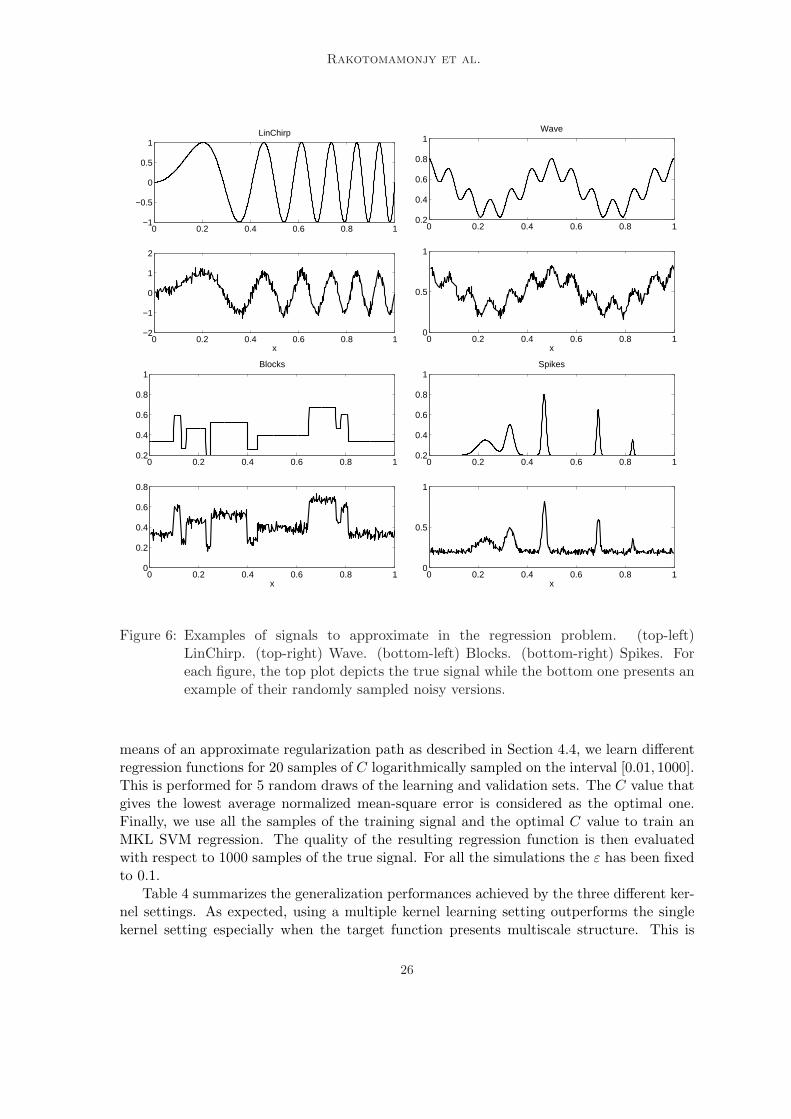
We applied this MKL SVM regression algorithm to simulated datasets which are well-known functions in the wavelet literature (Antoniadis and Fan, 2001). Each signal length is512 and a Gaussian independent random has been added to each signal so that the signal tonoise ratio is equal to 5. Examples of the true signals and their noisy versions are displayedin Figure 6. Note that the LinChirp and Wave signals present some multiscale featuresthat should suit well to an MKL approach.

Performance of the different multiple kernel settings have been compared accordingto the following experimental setting. For each training signal, we have estimated theregularization parameter C of the MKL SVM regression by means of a validation procedure.The 512 samples have been randomly separated in a learning and a validation sets. Then, by

25


0 0.2 0.4 0.6 0.8 1−1

−0.5

0

0.5

1LinChirp

0 0.2 0.4 0.6 0.8 1−2

−1

0

1

2

x

0 0.2 0.4 0.6 0.8 10.2

0.4

0.6

0.8

1Wave

0 0.2 0.4 0.6 0.8 10

0.5

1

x

0 0.2 0.4 0.6 0.8 10.2

0.4

0.6

0.8

1Blocks

0 0.2 0.4 0.6 0.8 10

0.2

0.4

0.6

0.8

x

0 0.2 0.4 0.6 0.8 10.2

0.4

0.6

0.8

1Spikes

0 0.2 0.4 0.6 0.8 10

0.5

1

x

Figure 6: Examples of signals to approximate in the regression problem. (top-left)LinChirp. (top-right) Wave. (bottom-left) Blocks. (bottom-right) Spikes. Foreach figure, the top plot depicts the true signal while the bottom one presents anexample of their randomly sampled noisy versions.

means of an approximate regularization path as described in Section 4.4, we learn differentregression functions for 20 samples of C logarithmically sampled on the interval [0.01, 1000].This is performed for 5 random draws of the learning and validation sets. The C value thatgives the lowest average normalized mean-square error is considered as the optimal one.Finally, we use all the samples of the training signal and the optimal C value to train anMKL SVM regression. The quality of the resulting regression function is then evaluatedwith respect to 1000 samples of the true signal. For all the simulations the ε has been fixedto 0.1.

Table 4 summarizes the generalization performances achieved by the three different ker-nel settings. As expected, using a multiple kernel learning setting outperforms the singlekernel setting especially when the target function presents multiscale structure. This is

26

SimpleMKL

Table 4: Normalized Mean Square error for the data described in Figure 6. The results areaveraged over 20 runs. The first column give the performance of a SVM regressionusing a single kernel which is the average sum of all the kernels used for the twoother results. Results corresponding to the columns Kernel Dil and Kernel Dil-Trans are related to MKL SVM regression with multiple kernels. # Kernel denotesthe number of kernels selected by SimpleMKL.

Single Kernel Kernel Dil Kernel Dil-TransDataset Norm. MSE (%) #Kernel Norm. MSE #Kernel Norm. MSELinChirp 1.46 ± 0.28 7.0 1.00 ± 0.15 21.5 0.92 ± 0.20

Wave 0.98 ± 0.06 5.5 0.73 ± 0.10 20.6 0.79 ± 0.07Blocks 1.96 ± 0.14 6.0 2.11 ± 0.12 19.4 1.94 ± 0.13Spike 6.85 ± 0.68 6.1 6.97 ± 0.84 12.8 5.58 ± 0.84

noticeable for the LinChirp and Wave dataset. Interestingly, for these two signals, perfor-mances of the multiple kernel settings also depend on the signal structure. Indeed, Wavepresents a frequency located structure while LinChirp has a time and frequency locatedstructure. Therefore, it is natural that the Dilation set of kernels performs better than theDilation-Translation ones for Wave. Figure 7 depicts an example of multiscale regressionfunction obtained when using the Dilation set of kernels. These plots show how the kernelweights adapt themselves to the function to estimate. For the same reason of adaptivityto the signal, the Dilation-Translation set of kernels achieves better performances for Waveand Spikes. We also notice that for the Blocks signal using multiple kernels only slightlyimproves performance compared to a single kernel.

5.3 Multiclass problem

For selecting the kernel and regularization parameter of a SVM, one usually tries allpairs of parameters and picks the couple that achieves the best cross-validation performance.Using an MKL approach, one can instead let the algorithm combine all available kernels(obtained by sampling the parameter) and just selects the regularization parameter bycross-validation. This last experiment aims at comparing on several multi-class datasetsproblem, these two model selection approaches (using MKL and CV) for choosing thekernel. Thus, we evaluate the two methods on some multiclass datasets taken from theUCI collection: dna, waveform, image segmentation and abe a subset problem of the Letterdataset corresponding to the classes A, B and E. Some information about the dataset aregiven in Table 5. For each dataset, we divide the whole data into a training set and atest set. This random splitting has been performed 20 times. For ease of comparisonwith previous works, we have used the splitting proposed by Duan and Keerthi (2005) andavailable at http://www.keerthis.com/multiclass.html. Then we have just computedthe performance of SimpleMKL and report their results for the CV approach.

27


0 0.2 0.4 0.6 0.8 11

2

3

4

5

6

7

8

9

10

11

x

Est

imat

ion

at a

giv

en le

vel

0 0.2 0.4 0.6 0.8 11

2

3

4

5

6

7

8

9

10

11

x

Est

imat

ion

at a

giv

en le

vel

Figure 7: Examples of multiscale analysis of the LinChirp signal (left) and the Wave signal(right) when using Dilation based multiple kernels. The plots show how eachfunction fm(·) of the estimation focuses on a particular scale of the target function.The y-axis denotes the scale j of the wavelet used for building the kernel. Wecan see that some low resolution space are not useful for the target estimation.

Table 5: Summary of the multiclass datasets and the training set size used.

Training Set SizeDataset #Classes # examples Medium LargeABE 3 2323 560 1120DNA 3 3186 500 1000SEG 7 2310 500 1000WAV 3 5000 300 600

In our MKL one-against-all approach, we have used a polynomial kernel of degree 1to 3 and Gaussian kernel for which σ belongs to [0.5, 1, 2, 5, 7, 10, 12, 15, 17, 20]. For theregularization parameter C, we have 10 samples over the interval [0.01, 10000]. Note thatDuan and Keerthi (2005) have used a more sophisticated sampling strategy based on acoarse sampling of σ and C and followed by fine-tuned sampling procedure. They alsoselect the same couple of C and σ over all pairwise decision functions. Similarly to Duanand Keerthi (2005), the best hyperparameter C has been tuned according to a five-foldcross-validation. According to this best C, we have learned an MKL all the full training setand evaluated the resulting decision function on the test set.

The comparison results are summarized on Table 6. We can see that the generaliza-tion performances of an MKL approach is either similar or better than the performanceobtained when selecting the kernel through cross-validation, even though we have roughlysearched the kernel and regularization parameter space. Hence, we can deduce that MKL

28

SimpleMKL

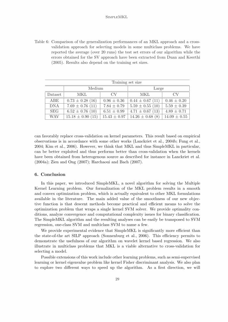
Table 6: Comparison of the generalization performances of an MKL approach and a cross-validation approach for selecting models in some multiclass problems. We havereported the average (over 20 runs) the test set errors of our algorithm while theerrors obtained for the SV approach have been extracted from Duan and Keerthi(2005). Results also depend on the training set sizes.

Training set sizeMedium Large

Dataset MKL CV MKL CVABE 0.73 ± 0.28 (16) 0.96 ± 0.36 0.44 ± 0.67 (11) 0.46 ± 0.20DNA 7.69 ± 0.76 (11) 7.84 ± 0.79 5.59 ± 0.55 (10) 5.59 ± 0.39SEG 6.52 ± 0.76 (10) 6.51 ± 0.99 4.71 ± 0.67 (13) 4.89 ± 0.71WAV 15.18 ± 0.90 (15) 15.43 ± 0.97 14.26 ± 0.68 (8) 14.09 ± 0.55

can favorably replace cross-validation on kernel parameters. This result based on empiricalobservations is in accordance with some other works (Lanckriet et al., 2004b; Fung et al.,2004; Kim et al., 2006). However, we think that MKL and thus SimpleMKL in particular,can be better exploited and thus performs better than cross-validation when the kernelshave been obtained from heterogenous source as described for instance in Lanckriet et al.(2004a); Zien and Ong (2007); Harchaoui and Bach (2007).

6. Conclusion

In this paper, we introduced SimpleMKL, a novel algorithm for solving the MultipleKernel Learning problem. Our formalization of the MKL problem results in a smoothand convex optimization problem, which is actually equivalent to other MKL formulationsavailable in the literature. The main added value of the smoothness of our new objec-tive function is that descent methods become practical and efficient means to solve theoptimization problem that wraps a single kernel SVM solver. We provide optimality con-ditions, analyze convergence and computational complexity issues for binary classification.The SimpleMKL algorithm and the resulting analyses can be easily be transposed to SVMregression, one-class SVM and multiclass SVM to name a few.

We provide experimental evidence that SimpleMKL is significantly more efficient thanthe state-of-the art SILP approach (Sonnenburg et al., 2006). This efficiency permits todemonstrate the usefulness of our algorithm on wavelet kernel based regression. We alsoillustrate in multiclass problems that MKL is a viable alternative to cross-validation forselecting a model.

Possible extensions of this work include other learning problems, such as semi-supervisedlearning or kernel eigenvalue problem like kernel Fisher discriminant analysis. We also planto explore two different ways to speed up the algorithm. As a first direction, we will

29


investigate ways to obtain a better the descent direction, for example with second-ordermethods. Note however that computing the Hessian needs the derivative of the dual variablewith respects to the weights d. This operation requires solving a linear system (Chapelleet al., 2002) and thus may produce some computational overhead. The second direction ismotivated by the observation that most of the computational load is to the computation ofthe kernel combination. Hence, coordinate-wise optimizers may provide promising routesfor improvements.

Acknowlegments

We would like to thank the anonymous reviewers for their useful comments. This workwas supported in part by the IST Program of the European Community, under the PAS-CAL Network of Excellence, IST-2002-506778. Alain Rakotomamonjy, Francis Bach andStephane Canu were also supported by French grants from the Agence Nationale de laRecherche (KernSig for AR and SC, MGA for FB).

References

A. Antoniadis and J. Fan. Regularization by Wavelet Approximations. J. American Sta-tistical Association, 96:939–967, 2001.

A. Argyriou, T. Evgeniou, and M. Pontil. Convex multi-task feature learning. MachineLearning, to appear, 2008.

N. Aronszajn. Theory of reproducing kernels. Trans. Am. Math. Soc., (68):337–404, 1950.

F. Bach. Consistency of the group Lasso and multiple kernel learning. Journal of MachineLearning Research, 9:1179–1225, 2008.

F. Bach, G. Lanckriet, and M. Jordan. Multiple kernel learning, conic duality, and the SMOalgorithm. In Proceedings of the 21st International Conference on Machine Learning,pages 41–48, 2004a.

F. Bach, R. Thibaux, and M. Jordan. Computing regularization paths for learning multiplekernels. In Advances in Neural Information Processing Systems, volume 17, pages 41–48,2004b.

M. Berkelaar, K. Eikland, and P. Notebaert. Lpsolve, Version 5.1.0.0, 2004. URL http://lpsolve.sourceforge.net/5.5/.

D. Bertsekas. Nonlinear programming. Athena scientific, 1999.

C. Blake and C. Merz. UCI repository of machine learning databases. University ofCalifornia, Irvine, Dept. of Information and Computer Sciences, 1998. URL http://www.ics.uci.edu/∼mlearn/MLRepository.html.

F. Bonnans. Optimisation continue. Dunod, 2006.

30

SimpleMKL

J.F. Bonnans and A. Shapiro. Optimization problems with pertubation : A guided tour.SIAM Review, 40(2):202–227, 1998.

J.F. Bonnans, J.C Gilbert, C. Lemarechal, and C.A Sagastizbal. Numerical OptimizationTheoretical and Practical Aspects. Springer, 2003.

S. Boyd and L. Vandenberghe. Convex Optimization. Cambridge University Press, 2004.

S. Canu, Y. Grandvalet, V. Guigue, and A. Rakotomamonjy. SVM and kernel methodsMatlab toolbox. LITIS EA4108, INSA de Rouen, Rouen, France, 2003. URL http://asi.insa-rouen.fr/enseignants/∼arakotom/toolbox/index.html.

C-C. Chang and C-J. Lin. LIBSVM: a library for support vector machines, 2001. Softwareavailable at http://www.csie.ntu.edu.tw/∼cjlin/libsvm.

O. Chapelle, V. Vapnik, O. Bousquet, and S. Mukerjhee. Choosing multiple parameters forSVM. Machine Learning, 46(1-3):131–159, 2002.

K. Crammer and Y. Singer. On the Algorithmic Implementation of Multiclass Kernel-basedVector Machines. Journal of Machine Learning Research, 2:265–292, 2001.

A. D’Amato, A. Antoniadis, and M. Pensky. Wavelet kernel penalized estimation for non-equispaced design regression. Statistics and Computing, 16:37–56, 2006.

A. D’Aspremont. Smooth Optimization with Approximate Gradient. SIAM Journal onOptimization, To appear, 2008.

D. DeCoste and K. Wagstaff. Alpha seeding for support vector machines. In InternationalConference on Knowledge Discovery and Data Mining, 2000.

K. Duan and S. Keerthi. Which Is the Best Multiclass SVM Method? An Empirical Study.In Multiple Classifier Systems, pages 278–285, 2005. URL http://www.keerthis.com/multiclass.html.

B. Efron, T. Hastie, I. Johnstone, and R. Tibshirani. Least angle regression (with discus-sion). Annals of statistics, 32(2):407–499, 2004.

G. Fung, M. Dundar, J. Bi, and B. Rao. a fast iterative algorithm for Fisher discriminantusing heterogeneous kernels. In Proceeedins of the 21th International Conference onMachine Learning, 2004.

Y. Grandvalet. Least absolute shrinkage is equivalent to quadratic penalization. In L. Niklas-son, M. Boden, and T. Ziemske, editors, ICANN’98, volume 1 of Perspectives in NeuralComputing, pages 201–206. Springer, 1998.

Y. Grandvalet and S. Canu. Adaptive scaling for feature selection in svms. In Advances inNeural Information Processing Systems, volume 15. MIT Press, 2003.

Y. Grandvalet and S. Canu. Outcomes of the equivalence of adaptive ridge with least absoluteshrinkage. MIT Press, 1999.

31


Z. Harchaoui and F. Bach. Image classification with segmentation graph kernels. In IEEEComputer Society Conference on Computer Vision and Pattern Recognition, 2007.

T. Hastie, S. Rosset, R. Tibshirani, and J. Zhu. The entire regularization path for thesupport vector machine. Journal of Machine Learning Research, 5:1391–1415, 2004.

C.-W. Hsu and C.-J. Lin. A comparison of methods for multi-class support vector machines.IEEE Transactions on Neural Networks, 13:415–425, 2002.

T. Joachims. Making large-scale SVM learning practical. In B. Scholkopf, C. Burges, andA. Smola, editors, Advanced in Kernel Methods - Support Vector Learning, pages 169–184.MIT Press, 1999.

S.-J. Kim, A. Magnani, and S. Boyd. Optimal kernel selection in kernel Fisher discrimi-nant analysis. In Proceedings of the 23rd International Conference on Machine Learning(ICML), 2006.

K. Koh, S.-J. Kim, and S. Boyd. An interior-point method for large-scale `1-regularizedlogistic regression. Journal of Machine Learning Research, 8:1519–1555, 2007.

G. Lanckriet, T. De Bie, N. Cristianini, M. Jordan, and W. Noble. A statistical frameworkfor genomic data fusion. Bioinformatics, 20:2626–2635, 2004a.

G. Lanckriet, N. Cristianini, L. El Ghaoui, P. Bartlett, and M. Jordan. Learning the kernelmatrix with semi-definite programming. Journal of Machine Learning Research, 5:27–72,2004b.

C. Lemarechal and C. Sagastizabal. Practical aspects of moreau-yosida regularization :theoretical preliminaries. SIAM Journal of Optimization, 7:867–895, 1997.

G. Loosli and S. Canu. Comments on the ”Core Vector Machines: Fast SVM Trainingon Very Large Data Sets”. Journal of Machine Learning Research, 8:291–301, February2007.

G. Loosli, S. Canu, S. Vishwanathan, A. Smola, and M. Chattopadhyay. Boıte a outilsSVM simple et rapide. Revue d’Intelligence Artificielle, 19(4-5):741–767, 2005.

D. Luenberger. Linear and Nonlinear Programming. Addison-Wesley, 1984.

C. Micchelli and M. Pontil. Learning the kernel function via regularization. Journal ofMachine Learning Research, 6:1099–1125, 2005.

A. Rakotomamonjy and S. Canu. Frames, reproducing kernels, regularization and learning.Journal of Machine Learning Research, 6:1485–1515, 2005.

A. Rakotomamonjy, X. Mary, and S. Canu. Non parametric regression with wavelet kernels.Applied Stochastics Model for Business and Industry, 21(2):153–163, 2005.

A. Rakotomamonjy, F. Bach, S. Canu, and Y. Grandvalet. More efficiency in multiple kernellearning. In Zoubin Ghahramani, editor, Proceedings of the 24th Annual InternationalConference on Machine Learning (ICML 2007), pages 775–782. Omnipress, 2007.

32

SimpleMKL

R. Rifkin and A. Klautau. In Defense of One-Vs-All Classification. Journal of MachineLearning Research, 5:101–141, 2004.

S. Rosset. Tracking Curved Regularized Optimization Solution Paths. In Advances inNeural Information Processing Systems, 2004.

B. Scholkopf and A. Smola. Learning with Kernels. MIT Press, 2001.

S. Sonnenburg, G. Ratsch, and C. Schafer. A general and efficient algorithm for multiplekernel learning. In Advances in Neural Information Processing Systems, volume 17, pages1–8, 2005.

S. Sonnenburg, G. Ratsch, C. Schafer, and B. Scholkopf. Large scale multiple kernel learning.Journal of Machine Learning Research, 7(1):1531–1565, 2006.

I. Tsochantaridis, T. Joachims, T. Hofmann, and Y. Altun. Large Margin Methods forStructured and Interdependent Output Variables. Journal of Machine Learning Research,6:1453–1484, 2005.

V. Vapnik, S. Golowich, and A. Smola. Support Vector Method for function estimation,Regression estimation and Signal processing, volume Vol. 9. MIT Press, Cambridge, MA,neural information processing systems, edition, 1997.

S. V. N. Vishwanathan, A. J. Smola, and M. Murty. SimpleSVM. In International Confer-ence on Machine Learning, 2003.

G. Wahba. Spline Models for Observational Data. Series in Applied Mathematics, Vol. 59,SIAM, 1990.

J. Weston and C. Watkins. Multiclass support vector machines. In Proceedings of ESANN99,Brussels. D. Facto Press, 1999.

A. Zien and C.S. Ong. Multiclass Multiple Kernel Learning. In Proceedings of the 24thInternational Conference on Machine Learning (ICML 2007), pages 1191–1198, 2007.

Appendix

Proof of convexity of the weighted squared norm MKL formulation

The convexity of the MKL problem (2) introduced in section 2.2 will be established ifwe prove the convexity of

J(f, t) =1t〈f, f〉H where f ∈ H and t ∈ R∗+

Since J(f, t) is differentiable with respects to its arguments, we only have to make surethat the first order conditions for convexity are verified. As the convexity of the domain ofJ is trivial, we verify that, for any (f, t) and (g, s) ∈ H × R∗+, the following holds:

J(g, s) ≥ J(f, t) + 〈∇fJ, g − f〉H + (s− t)∇tJ .

33


As ∇fJ = 2t f and ∇tJ = − 1

t2〈f, f〉H, this inequality can be written as

1s〈g, g〉H ≥ 2

t〈f, g〉H − s

t2〈f, f〉H ,

⇔ 〈t g − s f, t g − s f〉H ≥ 0 ,

where we used that s and t are positive. The above inequality holds since the scalar producton the left-hand-side is a norm. Hence problem (2) minimizes the sum of convex functionson a convex set; it is thus convex. Note that whenH is a finite dimension space, the functionJ(f, t) is known as the perspective of f , whose convexity is proven in textbooks (Boyd andVandenberghe, 2004).

Differentiability of optimal value function

The algorithm we propose for solving the MKL problem heavily relies on the differ-entiability of the optimal value of the primal SVM objective function. For the sake ofself-containedness, we reproduce here a theorem due to Bonnans and Shapiro (1998) thatallows us to compute the derivatives of J(d) defined in (10).

Theorem 1 (Bonnans and Shapiro, 1998) Let X be a metric space and U be a normedspace. Suppose that for all x ∈ X the function f(x, ·) is differentiable, that f(x, u) andDuf(x, u) the derivative of f(x, ·) are continuous on X × U and let Φ be a compact subsetof X. Let define the optimal value function as v(u) = infx∈Φ f(x, u). The optimal valuefunction is directionally differentiable. Furthermore, if for u0 ∈ U , f(·, u0) has a uniqueminimizer x0 over Φ then v(u) is differentiable at u0 and Dv(u0) = Duf(x0, u0).

34

SimpleMKL - Idiap Research Institute

Documents

Transcript of SimpleMKL - Idiap Research Institute