PR

IFY

SG

OL

BA

NG

OR

/ B

AN

GO

R U

NIV

ER

SIT

Y

Significance Testing Needs a Taxonomy

Bradley, Michael T.; Brand, Andrew

Psychological Reports

DOI:10.1177/0033294116662659

Published: 01/10/2016

Peer reviewed version

Cyswllt i'r cyhoeddiad / Link to publication

Dyfyniad o'r fersiwn a gyhoeddwyd / Citation for published version (APA):Bradley, M. T., & Brand, A. (2016). Significance Testing Needs a Taxonomy: Or How the Fisher,Neyman-Pearson Controversy Resulted in the Inferential Tail Wagging the Measurement Dog.Psychological Reports, 119(2), 487-504. https://doi.org/10.1177/0033294116662659

Hawliau Cyffredinol / General rightsCopyright and moral rights for the publications made accessible in the public portal are retained by the authors and/orother copyright owners and it is a condition of accessing publications that users recognise and abide by the legalrequirements associated with these rights.

• Users may download and print one copy of any publication from the public portal for the purpose of privatestudy or research. • You may not further distribute the material or use it for any profit-making activity or commercial gain • You may freely distribute the URL identifying the publication in the public portal ?

Take down policyIf you believe that this document breaches copyright please contact us providing details, and we will remove access tothe work immediately and investigate your claim.

18. Mar. 2020

Fisher, Neyman and Pearson Controversy 1

RUNNING HEAD: TAXONOMY RESOLVES THE FISHER, NEYMAN PEARSON

CONTROVERSY

Significance testing needs a taxonomy: or how the Fisher, Neyman-Pearson controversy resulted

in the inferential tail wagging the measurement dog.

Fisher, Neyman and Pearson Controversy 2

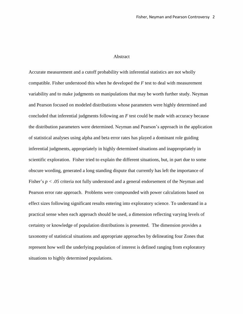
Abstract

Accurate measurement and a cutoff probability with inferential statistics are not wholly

compatible. Fisher understood this when he developed the F test to deal with measurement

variability and to make judgments on manipulations that may be worth further study. Neyman

and Pearson focused on modeled distributions whose parameters were highly determined and

concluded that inferential judgments following an F test could be made with accuracy because

the distribution parameters were determined. Neyman and Pearson’s approach in the application

of statistical analyses using alpha and beta error rates has played a dominant role guiding

inferential judgments, appropriately in highly determined situations and inappropriately in

scientific exploration. Fisher tried to explain the different situations, but, in part due to some

obscure wording, generated a long standing dispute that currently has left the importance of

Fisher’s p < .05 criteria not fully understood and a general endorsement of the Neyman and

Pearson error rate approach. Problems were compounded with power calculations based on

effect sizes following significant results entering into exploratory science. To understand in a

practical sense when each approach should be used, a dimension reflecting varying levels of

certainty or knowledge of population distributions is presented. The dimension provides a

taxonomy of statistical situations and appropriate approaches by delineating four Zones that

represent how well the underlying population of interest is defined ranging from exploratory

situations to highly determined populations.

Fisher, Neyman and Pearson Controversy 3

Significance testing needs taxonomy: or how the Fisher, Neyman-Pearson controversy resulted

in the inferential tail wagging the measurement dog?

A hallmark of science is measurement and measurement is characterized by accuracy and

precision. Probability estimates involve greater or lesser degrees of uncertainty, but statistical

procedures associated with inferential statistics for some characterize the scientific approach in

psychology (Babbie, 2001, p 452). These procedures have been extensively developed and are

influential in reporting the results of applied and behavioral studies. Great attention has been

paid to the correct mechanics of calculation, but somehow questions about the meaning of

significant results following of inferential tests while discussed by many (for examples, Cohen,

1994, Rosenthal, 1979, Sterling, 1959) have taken some time to have an impact. That impact has

possibly arrived with the American Statistical Association’s statements on p values (Wasserstein

and Lazar, 2016). Such papers, at the least, prime the field to ascertain how well probability

results reflect measurement accuracy.

Fisher recognized that results following an inferential test are the lowest level of

scientific inference (Box, 1978, pages 447-448). He distinguished different situations for the

judgment of results: 1) research involving exploratory scientific endeavors, and 2) statistics

associated with production processes and quality control. Exploratory research involves

inductive reasoning, and going from “consequences to causes” page 3, Fisher, 1942). Box

(1978, p 448) points out that statisticians looking for a single general solution and favoring

deductive reasoning were not satisfied with Fisher’s approach. Fisher offered a variety of

inferential approaches appropriate to some but not all problems. This was evident in the way

Fisher, Neyman and Pearson Controversy 4

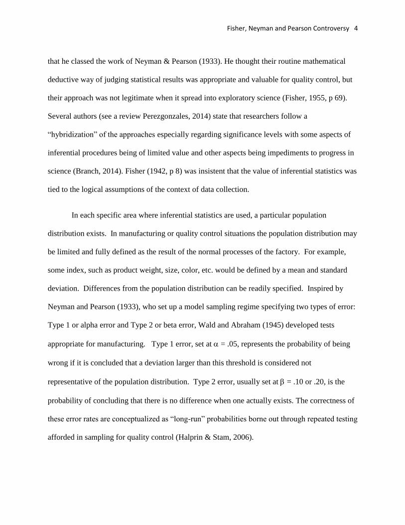
that he classed the work of Neyman & Pearson (1933). He thought their routine mathematical

deductive way of judging statistical results was appropriate and valuable for quality control, but

their approach was not legitimate when it spread into exploratory science (Fisher, 1955, p 69).

Several authors (see a review Perezgonzales, 2014) state that researchers follow a

“hybridization” of the approaches especially regarding significance levels with some aspects of

inferential procedures being of limited value and other aspects being impediments to progress in

science (Branch, 2014). Fisher (1942, p 8) was insistent that the value of inferential statistics was

tied to the logical assumptions of the context of data collection.

In each specific area where inferential statistics are used, a particular population

distribution exists. In manufacturing or quality control situations the population distribution may

be limited and fully defined as the result of the normal processes of the factory. For example,

some index, such as product weight, size, color, etc. would be defined by a mean and standard

deviation. Differences from the population distribution can be readily specified. Inspired by

Neyman and Pearson (1933), who set up a model sampling regime specifying two types of error:

Type 1 or alpha error and Type 2 or beta error, Wald and Abraham (1945) developed tests

appropriate for manufacturing. Type 1 error, set at = .05, represents the probability of being

wrong if it is concluded that a deviation larger than this threshold is considered not

representative of the population distribution. Type 2 error, usually set at = .10 or .20, is the

probability of concluding that there is no difference when one actually exists. The correctness of

these error rates are conceptualized as “long-run” probabilities borne out through repeated testing

afforded in sampling for quality control (Halprin & Stam, 2006).

Fisher, Neyman and Pearson Controversy 5

Fisher (1973) points out that the manufacturing situation contrasts with scientific

exploration. He states “… to identify a test of significance as used in the natural sciences with a

test for acceptance, one of the deepest dissimilarities lies in the population …used for making

statements of probability.(p 81)”. The true population distribution in science, at least at the outset

of exploration, is not known, and this contrasts with a well-described Neyman and Pearson type

of population. As a consequence with the exploratory population, one cannot with any certainty

suggest error rates in terms of alpha (Type 1) and beta (Type 2) probabilities. In other words, a

researcher divides a sample of the unknown larger population into groups some or one of which

is/are treated, and in that context the most legitimate judgment is categorical, depending upon the

probability level, in that groups are either like or unlike each other. Usually this is assessed by

mean differences, although other distribution qualities could be relevant (Bradley, Brand &

MacNeill, 2012, 2013; Tukey, 1977). That judgement for Fisher would be against the null

hypothesis if the probability was p ≤ .05. That such a treatment might work in another

circumstance is in all likelihood reasonable and all the more reasonable as the probability gets

smaller. It does not, however, yield something as definite as an error rate. If one does not know

the true population distribution, it is misleading to set error rates based on exploratory studies

and imply they have validity. Fisher made it clear that “… tests of significance which make a

dichotomy between hypotheses that are discredited by the data and those that are not…” are, as

mentioned earlier, the lowest level of scientific inference (Box, 1978, pages 447-448).

All samples of interest are a subset of the population distribution, and of course in that

sense the sample estimates approximate the parameters of population distribution. As Fisher put

it, sample values provide estimates of population parameters (Fisher, 1973, p 54).The sample,

however, (for example a particular University class) that any researcher may select could be

Fisher, Neyman and Pearson Controversy 6

substantially different from the more general population distribution of interest to the researcher

to begin with. For example, Sharpe and Poets (2015) reviewed the literature noting the paucity of

males in psychology experiments. Neyman and Pearson (1933) solved the sample - population

difference problem by making their population distribution the very one from which they were

sampling and resampling (Fisher, 1955). Thus, they could specify errors from their known

population. Fisher (1973, p 81) labeled them acceptance procedures for a product.

Fisher (1973, p 54-55) had, early in his career, introduced a fiducial approach to be

appropriate when no other information was available. This approach, borrowed from astronomy

and land surveying, establishes a reference point from which measurements are made (Stigler,

1986, p 101). The insight was that probability statements could be calculated within the data set

or sample at hand in just the same way that a path or acre could be measured off a fiducial point

in land survey. The limits, however, are two. In land survey the scale of measurement is of the

highest order, ratio scale (Stevens, 1946), whereas for Fisher the measurement in SD units is only

relevant to the sample, and the categorization of mean differences is dependent on probabilities

calculated on standard error (se) units. Thus the SD as a representative estimate is only as good

as the sample, and the se essentially supplies an increment that is the equivalent to a rubber ruler

that varies with the n. Thus, Fisher (1935) could only make categorical statements such as the

treated half of the sample is probably not like the untreated half of the sample. His probability

statements based on estimates from his initial sample were not exact to the population

parameters, but were predictive of future tests on samples of the same topic. In fact, Fisher

(1973) stated that “…the only populations that can be referred to in a test of significance have no

objective reality, being the product of the statistician’s imagination…(p 81)”. In other words, the

Fisher, Neyman and Pearson Controversy 7

researcher has no a priori knowledge of the center and shape of the imagined distribution. What

Fisher can conclude following a significance test “…of a small P-value is that something very

unlikely has happened or the null is false …” (Keuzenkamp and Magnus, 1995, p 18). Neyman

and Pearson believed they had defined a stable population distribution through repeated

sampling, whereas Fisher estimated the parameters of a fundamentally undefined population

distribution from the sample.

The argument is that the Neyman and Pearson model does not work in science. In

science the population parameters are not known, and the sample values are estimates of the

population imagined by the researcher. For Fisher (1973) differentiating between two groups in

a sample was valuable, but the most primitive form of measurement (p 46 …it is more primitive,

or elemental…). It has the status of furthering the inductive reasoning process but is not

definitive when trying to generalize to all members of a class or population. To make the

difference less abstract, consider the research concerns of Fisher such as manure on crops, or the

deterioration of food in storage (Fisher, 1973, p 79). With data, he could not say a program of

manure would be exactly as successful in a following year, but depending on the probability

levels, he could make a reasoned statement that this program is worth doing the following year.

With more research he could decide to look at different varieties of a crop, but until the

population is completely defined only probabilities, not error rates, can be reported. Fisher

(1973, 112-113) noted that a research scientist was dealing with inductive reasoning “…to

improve our understanding of the systems from which these observations are drawn”. Fisher

(1955, p 69) repeated this in an article on scientific induction as a major advantage to his and

Gosset’s approach (Student, 1908) in the introductory paragraph. Once the population

distribution is fully identified and specified then it is possible to apply the deductive approach

Fisher, Neyman and Pearson Controversy 8

favored by Neyman and Pearson (1933) with error rates (5% chance of Type 1 and a 10% or

20% chance of Type 2 error). Until then, however, the control sample is unspecified in its

approximation to the population distribution, and a specification of Neyman and Pearson errors

at this stage would refer only to the difference between the control and manipulated sample(s).

Error rates imply accuracy and precision that is unwarranted if someone applied the results to

another group from a different but as yet unknown sector of the population. With Fisher’s (1973,

p128) recommendation the report is of a result improbable by chance exactly between the groups

sampled and tested and in the early stages of research no more than that. Another researcher may

get a smaller or larger p, and over replications the extent of the difference and the likelihood of

that difference becomes known, maybe to the point with many samples where the Neyman and

Pearson’s approach applies. By then, Fisher (1973, p 80-81) would classify this as a use of

statistics valuable as “acceptance procedures” but not for scientific exploration.

In general, Fisher (1973, pages 80-81) described the difference between situations

(acceptance procedures) where an error approach referencing a known population distribution is

appropriate and where a probability approach identifying a difference between two distributions

is appropriate. This distinction anticipates a classification such that statistical approaches can be

placed on a dimension. This dimension classifies broad areas in which a researcher could make

a case for adopting particular form of judgment, error versus probability, appropriate for her/his

investigation. It is argued that an approach that differentiates various areas under study resolves

much of the controversy between Fisher and Neyman-Pearson. There are a variety of situations

in which probabilities are appropriate, but the choice of judging the meaning of the resultant

probabilities depends on what the researcher is examining.

Fisher, Neyman and Pearson Controversy 9

Fisher (1973, p 61) favored reporting exact p values that were calculated from specific

data sets being analyzed. He suggested distributions differed from each other when the

probability was less than .10 or .05 and became more confident that the distributions differed

with a lower p value such as .01 with the provision that “…no scientific worker has a fixed

level… (p 45)” for rejection. At higher levels of probability, he would simply withhold

judgment regarding whether the experimental variable failed to have an effect since “the null

hypothesis is never proved or established, but possibly disproved…” (Fisher, 1942, p 16).

Neyman and Pearson (1933) saw Fisher’s “no judgment possible” with regards to supporting the

null as unnecessarily limited.

Neyman and Pearson (1933) did not advocate reporting exact probabilities. Rather, they

suggested that that once the .05 level is crossed a decision to reject the null hypothesis will be

erroneous only one time in twenty. “In making decisions (a) or (b) we shall sometimes be in

error, for problems are rarely presented in such a form that we can discriminate with certainty

between the true and the false hypothesis. These errors will be of two kinds: (I) we reject Ho

when it is true, (II) we accept Ho when some alternative Hi is true. The problem before us is to

consider how these errors may be. In a reciprocal fashion, if the beta error rate is low, .10 or

less, then the acceptance of the null hypothesis through a failure to find significance would result

in an error only 1 in ten times” (page 493).

In sum inferential statistics can be used either for monitoring or for research, but which

depends upon whether the results are judged by error rates or probabilities. A researcher can

reason from probability judgements as to whether there is enough evidence to pursue a

phenomenon of potential interest and are not designed for accurate and precise measurement

Fisher, Neyman and Pearson Controversy 10

(Fisher, 1955, p 73). A small probability simply says that two or more samples differ to such a

degree that one or more samples is/are not like the reference sample. Any particular effect size

calculated to reflect differences between the distributions could be accurate, but in general the

average calculation of a set of effect sizes following inferential statistics will not be accurate if

power is less than an impossible 100% with the standard criterion of p ≤ .05 applied as a cutoff

value. Accuracy is the closeness of a measured result to the true underlying value and to the

degree that a significant result is inaccurate effect size measures will be inaccurate through

exaggeration.

Precision or imprecision is a little more difficult to gauge. Underpowered studies, if

published under .05 alpha constraints, inherently produce inaccurate estimates if effect sizes are

calculated (for examples of discussion, Bakan 1966, Brand, Bradley, Best, and Stoica, 2008,

Cohen, 1994, Gigerenzer, 1993, Kline, 2013). Even under the best of circumstances (90% power,

a normal distribution), Bradley and Brand (2016) showed with Monte Carlo results that the

probability estimates from inferential statistics are 6% larger than the actual value tested.

Further and pertinent to precision, these estimates would probabilistically be around the .05 level

and could appear deceptively precise if the studies had approximately the same sample size. Of

course, if there were a variety sample sizes in underpowered studies, the estimates would vary.

Currently the publication manual of the American Psychological Association helps remedy this

problem by suggesting the calculation of effect sizes and CIs associated with non-significant

results (APA manual 6th ed, 2010, p 33). There has been a definitive change as the 4th edition

only encouraged effect size reporting, and the 5th edition indicted that a fuller understanding of

the results would be conveyed if the effect sizes were reported (APA manual 4th & 5th eds, 1999,

2002). If the suggestions of the 6th edition are followed, which include even non-significant

Fisher, Neyman and Pearson Controversy 11

effect size reporting, the CIs would be more legitimate reflections of the set of effect sizes. If,

however, the bias towards focusing on effect sizes calculated after significance remains, then the

CIs for generally underpowered studies would be particularly distorted if the sample sizes in the

set of studies varied substantially (Bradley & Stoica, 2004, Brand & Bradley, 2016). Of course

once the probability screening criteria is dropped, it is no longer inference but becomes

measurement.

Fisher saw inferential tests and particularly the F test as useful but the most rudimentary

of measurement tools (Box, 1978, pages 447-448). . They simply allowed the basic judgment of

whether a new sample conformed to or deviated from the reference or null distribution. He and

any researcher could state this in probability terms, as had been done previously by others using

the term probable error (Cowles, & Davis, 1982). Initially, he was fairly casual about the famous

p ≤ .05 level. In fact, he said that those who insisted on the .05 level did not know statistics:

“…significance… is more primitive, or elemental than, and does not justify, any exact

probability statement about the proposition (Fisher, 1973, p 46).” The quote is key to the

controversy, because Neyman and Pearson (1933) were making exact statements. Fisher

entertained a variety of potential significance levels depending upon the experimental

circumstance, sample sizes, and distribution moments. He gave prominence to the .05 level, but

it was mentioned in the context where .10 could be of interest depending on the circumstance.

He did balance his thoughts by mentioning p < .01 as a hard criteria to meet and strongly

suggestive of support for a phenomenon, and then came back to .05 as worthwhile to promote

further investigation. Perhaps Fisher succinctly phrased it with “…no scientific worker has a

fixed level of significance at which from year to year, and in all circumstances, he rejects

hypotheses; he rather gives his mind to each particular case in the light of the evidence and his

Fisher, Neyman and Pearson Controversy 12

ideals.” (Fisher, 1973, p 45). In specific regards to non-significance Fisher (1955) said, “The

deviation is in the direction expected…and to this extent my suspicion has been confirmed…the

data available….is not … sufficient to demonstrate their reality.” p73). As an area is known then

“…a properly designed experiment rarely fails to give this level of significance…” (Fisher 1926,

p 504, original author emphasis). It is notable that Fisher wanted the exact level of p reported for

each replication attempt, assuming a somewhat consistent and reasonable sample size for each

experiment, and by reasonable we mean a sample size likely to yield statistically significance

results. Fisher’s views are harmonious with current APA (2010) recommendations.

In 1935 Neyman orally presented a paper with Fisher in the audience meant to “…rectify

the deficiencies of Fisher’s thought” (Box, 1978, p263). Fisher (1955) said that Neyman “denies

the existence of inductive reasoning” (p 74) and thought in terms of deductive reasoning. He

with Pearson meant to sharpen the accuracy of Fisher’s technique by considering situations

where the populations of interest were limited and could be specified with exactitude. As

mentioned Wald and Abrahamson (1945) applied the reasoning to quality control situations

where inputs can be standardized and controlled. A context such as that comes pretty close to

meeting scientific criteria for measurement. Thus, Neyman and Pearson’s approach has been

appropriately applied to production lines, because the production process determines with

exactitude the input, and the physical or qualitative aspects of the final product can be specified

in measureable terms (Lenhard, 2006). In addition, production processes involve reiteration or

multiple opportunities for replication. With such knowledge, a sampling routine with

probabilistic expectations of finding deviations from the expected product can be set up. The

issue in this context is to discover a sample size that could in turn discover deviations with only a

5% chance that any particular deviation of that magnitude did not represent some problem with

Fisher, Neyman and Pearson Controversy 13

the production process and an 80% or 90% chance of discovering the deviation that reflected the

problem. Of course, these values represent alpha or Type 1 error rates and the 10% or 20%

(power, 100% - 90% or 80%) reflects the beta or Type 2 error rate. With several tests a number

reflecting “normal” production processes deviations from normal could be derived such that a

decision to 1) continue or 2) check the process could be made. A production process involves a

well determined model with known properties. It is an appropriate application of technology. It

is not the generation of new facts or “an intelligent attempt to understand the experimental

situation.” (Fisher, 1955, p77, original author emphasis). The reason it is not “exploratory

science” is that Neyman and Pearson’s distribution is limited to a distribution that can be

completely known. Importantly, that distribution does not pertain to all distributions of that type,

because if, for example, a new manufacturing process were set up a new distribution associated

with indices of the product would have to be explored.

The Neyman and Pearson approach of specification of Type 1 and Type 2 error rates can

be done legitimately if virtually all aspects of the data gathering situation are determined. What

Neyman and Pearson are really assuming is that a priori they know all about or enough about the

reference distribution that they can, with small probabilities of error, suggest when a measured

distribution deviates from or remains within the parameters of that distribution. In such

circumstances, inferential statistics may become unnecessary and tolerance numbers derived

from exact estimates of effect size may indicate the soundness of a process. For example, if a

product should have a certain weight, a certain number of deviations from that weight may

reflect a production problem.

Fisher, Neyman and Pearson Controversy 14

When the population distribution from which the sample is drawn are unknown it is not

possible to specify population probabilities as error rates. Fisher (1973) put it clearly many times

“…the evidence available concerns one population only, and tells us nothing more of the parent

population that might lie behind it…(1973, p 124, for example)” The model of the reference

distribution only emerges after the data has been collected, and it is only possible to infer if a

difference between the reference distribution and a particular comparison distribution is

improbable enough to make the pursuit of further investigation potentially worthwhile. David

and Edwards (2001, p 188) also stated Fisher’s notion clearly “…a probability statement about a

parameter based on a fiducial distribution has the same inductive content as if the parameter had

been drawn at random from a conventional probability distribution of identical form…” What

makes the Neyman-Pearson testing situation so different is the assumption that the distribution

sampled from is always the same known distribution, which is true in the context of product

testing, but specifically not in exploratory situations. Fisher’s problem was how to make

“…inferences from the particular to general…” from variable data (Box, 1978, p 447). He was

unsettled that advocates of the Neyman and Pearson approach did not seem to make a distinction

between technical measurement and scientific exploration. If a distribution is defined

beforehand “Nothing essentially new can be discovered…” (Fisher, 1973, p 112). This was

unsettling because in his early surmise of his contribution Fisher (1922, p323) had noted “…the

number and variety of the new results the method discloses…”).

Fisher’s choice of words to describe his points could result in problems. He used

“imaginary” and “fiduciary”. “Imaginary” referred to the underlying population that the

researcher had in mind for generalization (Fisher, 1955, p71). A researcher can only sample from

Fisher, Neyman and Pearson Controversy 15

the population in mind with the particular portion of the population at hand. This leads to

“fiduciary” probabilities or probabilities in reference to the sample being analyzed (Fisher,

1935). A researcher does not have an entire defined population. She/he has only a particular part

of the population to sample from, in Fisher’s case, a particular wheat field in England. The

estimates from the sample serve as reference or fiducial points and may or may not adequately

generalize to the “imagined” population (all wheat fields in England, the world?). An

experiment is an instance to be generalized, but “The governing characteristic of inductive

reasoning is that it is always used to arrive at statements of uncertainty… (Fisher 1973, p113).

Fisher could agree that the generalization may be reasonable depending on a p value following a

manipulation, but Fisher would never agree that error probabilities had been legitimately

specified with respect to the abstract population to which a researcher “imagined” the results

pertained.

Fisher tried to explain the difference between his approach and that of Neyman and

Pearson. P values are not error rates, rather they indicate the probability that data after a

treatment are like data from an untreated sample. The smaller the p the more likely the treated

sample is different than the untreated or null sample. Fisher (1973, p81) made it clear that

identifying significance testing in science with an acceptance test in production fails to recognize

the deep dissimilarity “…in the population, or reference set, available for making statements of

probability …”. Fisher complained that Neyman and Pearson had been insulated from natural

science (Fisher, 1955, p 70), and thus they failed to understand the tentative or exploratory nature

of the few samples obtained in any given area.

Fisher, Neyman and Pearson Controversy 16

Perezgonzales (2014) is one of many who have noted that there is a danger in using a

hybrid conception of inferential statistical testing. There are problems, Perezgonzales noted, if

probabilities are treated as error rates: effect sizes are calculated, confidence intervals reported,

and power is calculated all from a small set or even a singular exploratory study. All of these

practices can only be justified on the bases of positing a stable reference distribution and cannot

be justified on the basis of a “fiduciary” or a benchmark reference distribution. Brand, Bradley,

Best, and Stoica, (2008) reported that exaggerated results may be published. Improbable

significant findings represent some of the literature, whereas the unpublished failures comprise

the now famous/infamous “file drawer” (Rosenthal, 1979).

Publishing practice in psychology as recommended by American Psychological

Association (APA) manuals from the 1940s until the 1990ties directed researchers to indicate

significance at the .05, .01, or .001 level without discussing whether these values were error rates

or probabilities. Following Fisher’s probability model a researcher would report an exact

probability with the implication that smaller probabilities are better. Fisher was not stating that

he “knew” all the characteristics of the reference distribution. Rather the sample was merely a

sample that more or less approximated the population distribution, and, as such, it would be

inappropriate to calculate an effect size if the inferential test is underpowered and involves a

“fiduciary” or “convenient benchmark” distribution. Following the practice of reporting effect

sizes in such circumstances, results in unstable (imprecise) estimates that are likely to be

exaggerations (inaccurate) in the published literature.

The APA manual (2010) suggests reporting Confidence Intervals (CIs). CI calculations

involve an inferential approach since the calculation of CIs is based on the standard error. Thus

Fisher, Neyman and Pearson Controversy 17

NHST and CIs depend upon the sample size in any particular area, and since sample sizes can

vary, it is analogous to using an elastic band as a ruler. Thus, significance comes and goes, and

worse, in some areas the only calculations of effect sizes may come from misestimates of mean

differences, variability, or a combination of both. An additional problem is that confidence

intervals are often huge and exceed the magnitude of the effect size they are meant to bracket

(Brand and Bradley, 2016). This results in a peculiar problem. If replication involves obtaining

a value less than alpha, it is difficult to obtain results. If replication involves fitting in the

confidence interval, it is difficult to fail to replicate (Brand & Bradley, 2016).

The Fisher, Neyman and Pearson controversy can be portrayed as part of a larger

dimension of probability testing. This dimension includes classical probability, well defined

distributions, and exploratory science. Between exploratory science and well defined

distributions there is a transition zone where shared characteristics of both exploration and

knowledge co-exist. The dimension is multifaceted ranging from substantial but not perfect

certainty to great uncertainty; deductive reasoning to inductive reasoning; described probabilities

to estimated probabilities. Zone 1, or the approximate certainty end of the dimension, is

characterized by classical probability; Zone 2 is best related to technological processes; Zone 3 is

a middle ground with some but not complete knowledge; and Zone 4 involves exploratory

science. Zone 3 follows Hulbert and Lombardi (2009). In this middle ground, researchers have

some knowledge but they do not know the exact size of an effect or whether they have an

adequately sized population to test an effect. In such cases, a researcher could allow a more

liberal p value to continue work or to entice others to contribute more data. Bradley and Brand

(2013) published a set of tables with small, medium and large effects, varying levels of power,

and varying Ns to show the alpha level that is expected given those parameters. If the theory is

Fisher, Neyman and Pearson Controversy 18

dealing primarily with an established effect, but there are other potential effects of interest, then

more liberal alphas levels could allow the entry of this less conclusive but possibly important

subsidiary data into a field. We should point that other fields are working along similar lines.

Mudge, Baker, Edge, and Houlahan (2012) combined Type 1 and Type 2 error rates to arrive at

an optimal alpha both retrospectively for completed studies and prospectively for “to be

conducted” work. If either or both of these approaches become widely accepted, they will

reduce the volume of studies in the “file drawer” and increase the availability of more accurate

effect size estimates. In addition, it can be argued that both Fisher and Neyman and Pearson had

a nascent appreciation of this middle ground we call Zone 3. Neyman and Pearson clearly

indicated that at times avoiding a type 2 error was more important than guarding against a type 1

error. Fisher suggested that “sometimes” depending on the subject and context a more liberal

alpha probability indicating a difference was acceptable.

With a dimension and zones a user of inferential statistics can identify which zone they

are working in. If you can control production processes to the point that you control even the

materials fed into the process, you are working in the Neyman-Pearson area or Zone 2. You may

design such a stable production process that a criteria set by a particular number of errors may

obviate the need for statistical testing. This is because the characteristics of the reference

distribution are controlled entirely by the process. For deductive reasoning, an error-based

decision is valuable in this context. If the quality assessment is within a certain range, then it is

reasonable to continue on producing. If it is out of the range, the “behavior’ would be to shut

production down with a 5% chance of error. Such decisions can only be achieved if the

population distribution is thoroughly known, as it would be in a particular factory with a

Fisher, Neyman and Pearson Controversy 19

particular product. Fisher (1955, p 69) himself recognized the value of “acceptance” procedures

reflecting upon his air travel, but he rejected these same procedures for science.

If you don’t have much knowledge or only a hypothesis as to what the input or outcome

of a study will be you are at the Fisher extreme or Zone 4. The key is that not only do you not

control the population distribution you do not even have much knowledge about its

characteristics. As such, you can take samples from it, and these samples, of course, are part of

the larger population, but it is not known which part. These samples, of course, converge on an

actual population distribution, but they only represent that distribution in a probabilistic way.

Thus, the local population distribution is likely the one that is convenient but not necessarily

universal. The uncertainty about distributional qualities allows the conclusion that a

manipulation alters a sample so that it no longer looks like the unmanipulated distribution. It

does not specify the difference in terms of the universal population distribution which may not

exist.

A researcher may to move into middle ground or Zone 3 after several experiments, but

that happens only after enough attempts to estimate parameters of a distribution are conducted.

Once a researcher has gained enough knowledge to move into the middle zone, judgments about

distributional characteristics should be made with more accuracy.

From our understanding, neither Fisher’s or Neyman and Pearson’s approach fit well into

Zone 3. Fisher did, as mentioned, suggest a liberal p is possible to accept for investigation, but

in the main with a multitude of potential hypotheses, his interest at the time was in pursuing

something that was likely obvious in a probabilistic sense. We had placed Neyman and Pearson

firmly in Zone 2 with the specification of a distribution gained through control and verified

through reiterated samples. This procedure allows the estimation of probabilities of Type 1 and

Fisher, Neyman and Pearson Controversy 20

Type 2 errors for making decisions about a sample, but as we argued earlier Neyman and

Pearson encroach upon Zone 3 with the recognition that for errors sometimes “… it will be more

important to avoid the first, in others the second” (Neyman and Pearson, 1933, p 296). In

general, however, they made strong statements that Type 1 errors were more problematic “…an

error of the first kind is more important to avoid than an error of the second kind…” (Neyman,

1950, p 265).

Theory and measurement are primary. An inference (the use of inferential statistics on

measured values) about measurement is secondary. That inference may, in the absence of other

information, signal something about the probability of the results, but replication with the

admission of all legitimate attempts to replicate is the most reasonable way to establish and

understand a finding. However, we also accept that inferential statistics can facilitate judgment if

used properly. The dimension of “zones” to portray a model that guides researchers towards the

correct application of inferential statistics.

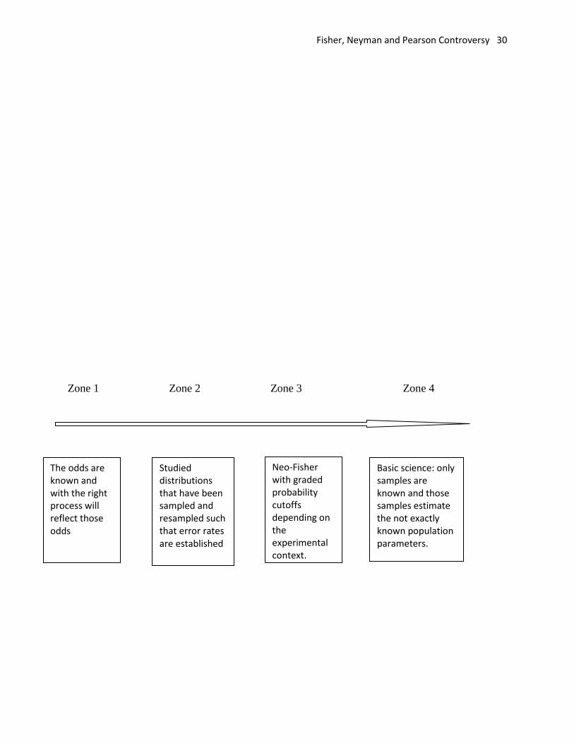
The diagram represents four zones along a dimension of certainty, where certainty refers

to the degree to which the inferential evaluative situation is fully defined. The zones are not

mutually exclusive and it would take some experience or knowledge of an area to make some

distinctions at the borderlines.

-------------------------------------------------------------------------------------

Figure 1 about here

--------------------------------------------------------------------------------------

Fisher, Neyman and Pearson Controversy 21

Zone 1 consists of classic probability. Essentially the data is categorical and certainty is

virtually assured in the long run. There is, of course, some uncertainty related to improbable

outcomes until a final outcome is achieved.

Zone 2 consists of Neyman and Pearson’s attempt to create a situation in which virtually

everything about the reference distribution is known. Production is perhaps the easiest example

since virtually every variable such as the input materials, the length of the process, the

temperatures, and the skill of the labor is controlled. Depending on the complexity of the

process, inferential tests at various levels in the process reveal problems that may arise. The

complexity of potential questions is substantial. As mentioned, Fisher said inferential statistics

are the most primitive form of measurement. As more is known about the area more

sophisticated forms of measurement can be brought to bear. He argued that for production lines

Neyman and Pearson were following an appropriate model, but, as we agree, that model creates

problems for the conduct of science (Fisher, 1955, p 69).

Zone 3 will be discussed after zone 4 because some of the conceptual orientation comes

from zone 4.

Fisher described and designed statistics for Zone 4. He wanted to make a rough and ready

distinction between those areas that were worth pursuing and those which were more ambiguous.

Fisher developed his ideas prior to modern calculators and computers, where analyses were

laborious. Allocating his time to various problems was a real decision. He studied wheat, which

could vary each year depending upon wind, rain, sun and temperature as well as soil and disease

infestations. Thus, his reference distribution varied, and the question is: did the comparison

distribution also vary enough from the reference to suggest that one type of wheat was

Fisher, Neyman and Pearson Controversy 22

superior/inferior to another? On the one hand, he had to make a decision so he had in mind some

criteria such as p < .05 or less, but, on the other hand, there could be circumstances in any given

year that would allow a more liberal cutoff such as p < .10. He advocated the use of judgment in

making these decisions. A researcher does not have an idea until the data are collected of the

form of the distributions and the measure of central tendency. Ceiling or floor effects reflected

in skewness could be operative and be taken into account by a researcher. His idea of reporting

exact p values reflected an attempt to gauge precision. Hubbard and Bayyarri (2003) point out

that Fisher had a conception of the true population distribution of which he only had a sample,

and then the question becomes whether the manipulated distribution was compatible or not with

that null. The more the samples differ the greater the probability they will differ again even in a

new context, and over time with consistent low p values a fact might be established.

Zone 3 emphasizes the use of judgment depending upon what one is studying. An

estimate of harm potential has been a factor in clinical drug tests. For example, Bendtsen, Bigal,

Cerbo, Diener, Holroyd, Lampl, Mitsikostas, Steiner and felt-Hansen (2009) suggest a great

many factors from drug interactions, functional impairment, to toxicity that need to be monitored

and reported numerically and possibly a liberal p value to be alert for harm. If undiscovered in

initial testing, they may become obvious in larger clinical samples. If a more liberal p value

pertained in the initial tests, a researcher could have an awareness of potential side effects.

Fisher argued that his samples were only a sample of the possible/hypothetical

population. His particular wheat fields in England belong to a limited population of wheat fields.

He wanted his data to generalize to wheat all over England. A substantial difference between his

reference sample and his tested sample, reflected in a lower p value, is more likely to generalize.

Fisher, Neyman and Pearson Controversy 23

From the perspective of pre-computer or early computational aids and a limited number of

statistical tests, it is reasonable to look for phenomena that have substantial effects. Fisher

recognized the unknown nature of his actual population.

Neyman and Pearson (1933) were correct for recognizing that Fisher’s procedures could,

both in theory and empirically in very limited situations, model a situation in which the distance

between means are described not only with very little chance of error but almost with exact

specification of potential error. They also are correct since quality testing had long ago emerged

(Student, 1908), for the clear applicability of their error decision model.

The current application of inferential statistics involve a hybrid model of NHST practice

(Gigerenzer, 1993). Computing power and a massive numbers of research projects (Bradley &

Gupta, 1997) using inferential statistics in what Gigerenzer termed a “ritualistic” manner have

created problems for psychology. We have no evidence that Fisher in setting low p values

anticipated 125,000 Psychologists in North America, plus some large number of Psychologists

around the world who also have graduate and honors students, plus professors of Business,

Biology, Education, Pharmacology, Nursing, etc, plus all of their students. Brand, Bradley, Best

and Stoica (2008) showed with a small effect size tested with typical sample size would be

significant yielding a Type 1 error once in seven tests and thus have an opportunity for

publication. For every million researchers, roughly 140,000 papers of dubious value could be

generated, and with a 10 to 20% percent acceptance rate as many as 28,000 papers could show

up across the various disciplines. Our scenario only portrays a limited sample of the potential

magnitude of the problem. Add to these erroneous findings as Gigerenzer points out, a feeling of

confidence emanating from abuse of the Neyman and Pearson model. That is with power

Fisher, Neyman and Pearson Controversy 24

calculations based on previous exaggerated estimates, a statistically rare (Type 1) phenomena

seems supported. The illusion of a supportable finding occurs because of ‘the file drawer effect

and the number of industrious participants most of whom file away their non-significant results

while the fewer Type 1errors are published. A researcher, reader and editor could have false

confidence in an apparently low probability event with seemingly adequate power to find it.

It is unfortunate that neither Fisher or Neyman and Pearson could anticipate the

popularity of their methods and the mechanistic ways of application. Fisher had mapped clearly

two of our zones and would clearly support the use of Neyman and Pearson methods in Zone 2

while insisting on the application of his approach in Zone 4. Neyman and Pearson definitely

were successful in defining Zone 2 and showed signs of thinking about Zone 3 with a more

liberal alpha when power was not optimal. Both Fisher and Neyman and Pearson have been

victims of their own success.

Fisher, Neyman and Pearson Controversy 25

References

American Psychological Association. (1999). Publication manual of the American Psychological

Association (4th ed.). Washington, DC: Author.

American Psychological Association. (2002). Publication manual of the American Psychological

Association (5th ed.). Washington, DC: Author.

American Psychological Association. (2010). Publication manual of the American Psychological

Association (6th ed.). Washington, DC: Author.

Babbie, E. R. (2001). The practice of social research. (9th ed.) Wadsworth: Belmont Ca.

Bakan, D. (1966). The test of significance in psychological research. Psychological Bulletin,

66, 423–437.

Bendtsen, L., Bigal, M. E., Cerbo, R., Diener, H. C., Holroyd, K., Lampl, C., Mitsikostas, D.D.,

Steiner, T.J. & Tfelt-Hansen, P. (2009) Guidelines for controlled trials of drugs in

tension-type headache: Second edition. Cephalalgia 30(1) 1–16

Box, J. F. (1978). R. A. Fisher: the life of a scientist. John Wiley

Bradley, M. T. & Brand, A. (2013). Alpha values as a function of sample size, effect size, and

power: accuracy over inference. Psychological Reports: Measures & Statistics, 112, 3, 1-

10.

Bradley, M.T. & Brand, A. (2016). Accuracy when inferential statistics are used as

measurement tools. BMC Research Notes20169:241. DOI: 10.1186/s13104-016-2045-z

Bradley, M. T., Brand, A., & MacNeill, A. L. (2012). Interpreting effect size estimates through

graphic analysis of raw data distributions. In Cox, P. Rodgers, P. & Plimmer, B. (Eds)

Diagrams. 117-123. Springer-Verlag: Berlin.

Fisher, Neyman and Pearson Controversy 26

Bradley, M. T., Brand A., & MacNeill, A. L. (2013, June). Effect size reporting reveals the

weakness Fisher believed inherent in the Neyman-Pearson approach to statistical

analysis. Poster presented at the annual meeting of the Canadian Psychological

Association. Quebec City, Quebec

Bradley, M. T. & Gupta, R. D. (1997). Estimating the effect of the file drawer problem in meta-

analysis. Perceptual & Motor Skills, 85, 719-722.

Bradley, M. T. & Stoica, G. (2004). Diagnosing estimate distortion due to significance testing in

literature on the detection of deception. Perceptual and Motor Skills, 98(3), 827–839. doi:

10.2466/Pms.98.3.827–839

Branch, M. (2014). Malignant side effects of null-hypothesis significance testing. Theory &

Psychology, 24, 256-277.

Brand, A., Bradley, M. T., Best, L., & Stoica, G. (2008) Accuracy of effect size estimates from

published psychological research. Perceptual & Motor Skills, 106, 645- 649.

Brand, A., & Bradley, M. T. (2016) The Precision of Effect Size Estimation From Published

Psychological Research Surveying Confidence Intervals. Psychological Reports 118,

1 154-170. doi: 10.1177/0033294115625265

Cohen, J. (1994). The earth is round (p < .05). American Psychologist, 49, 997–1003.

Cowles, M. & Davis, C. (1982). On the Origins of the .05 Level of Statistical Significance.

American Psychologist. 37, 5, 553-558

David, H. A. and Edwards, A. W. F. (2001). Annotated Readings in the History of Statistics.

Springer, New York.

Fisher, R. A. (1922). On the Mathematical Foundations of Theoretical Statistics. Philosophical

Fisher, Neyman and Pearson Controversy 27

Transactions of the Royal Society of London 222, 309-368.

Fisher, R. A. (1925). Statistical methods for research workers. Oliver & Boyd: Edinburgh.

Fisher, R. A. (1926). The arrangement of field experiments. Journal of the Ministry of

Agriculture, 33, 503-513.

Fisher, R. A. (1935). Statistical Tests. Nature, 136, 474.

Fisher, R. A. (1942). The design of experiments. (3rd ed.) Oliver & Boyd: London.

Fisher, R. A. (1955). Statistical methods and scientific induction. Journal of the Royal Statistical

Society. Series B (Methodological) 17, 1, 69-78.

Fisher, R. A. (1973). Statistical methods and scientific inference. (3rd ed.) Hafner Press: New

York.

Gigerenzer, G. (1993). The superego, the ego, and the id in statistical reasoning. In G. Keren, &

Lewis. (Eds.), A Handbook for Data Analysis in the Behavioral Sciences:Methodological

Issues (pp. 311-339). Hillsdale, New York: Lawrence Erlbaum Associates.

Halprin, P. F. & Stam, H. J. (2006). Inductive inference or inductive behavior: Fisher and

Neyman-Person approaches to statistical testing in psychological research (1940-1960).

The American Journal of Psychology, 119, 625-653.

Hubbard, R. & Bayarri, M. J. (2003). Confusion over measures of evidence (p’s) versus errors

(a) in classical statistical testing. The American Statistician, 57, 171-182.

Fisher, Neyman and Pearson Controversy 28

Hurlbert, S. H. & Lombardi, C. M. (2009). Final collapse of the Neyman-Pearson decision

theoretic framework and the rise of the neoFisherian. Annales Zoologic Fennici, 46, 311-

349.

H.A. Keuzenknmp, H. A, & Magnus, J.R. (1995) Journa1 of Econometrics 67, 5-24.

Kline, R. B. (2013). Beyond significance testing: Statistics reform in the behavioral sciences

(2nd ed.). Washington, DC: American Psychological Association.

Lenhard, J. (2006). Models and Statistical Inference: The Controversy Between Fisher and

Neyman–Pearson. British Journal for the Philosophy of Science 57 (1):69-91. doi:

10.1093/bjps/axi152

Mudge, J. F., Baker, L. F. Edge, C. B., Houlahan, J. E. (2012). Setting an optimal α that

minimizes errors in null hypothesis significance tests. PLoS One;7:e32734

Neyman, J. & Pearson, E. S. (1933). On the Problem of the Most Efficient Tests of Statistical

Hypotheses. Philosophical Transactions of the Royal Society A: Mathematical, Physical

and Engineering Sciences 231 (694–706): 289–337. doi:10.1098/rsta.1933.0009

Neyman, J. (1937). Outline of a theory of statistical estimation based on the classical theory of

probability. Philosophical Transactions of the Royal Society A 236: 333–380.

Neyman, J. (1950). First Course in Probability and Statistics. New York: Henry Holt.

Perezgonzales, J. D. (2014) A reconceptualization of significance testing. Theory &

Psychology, 24: 852-859, doi:10.1177/0959354314546157

Rosenthal, R. (1979). "The "File Drawer Problem" and the Tolerance for Null Results",

Psychological Bulletin 86 (3): 638–641, doi:10.1037/0033-2909.86.3.638

Fisher, Neyman and Pearson Controversy 29

Salsburg, D. (2001) The Lady Tasting Tea: How Statistics Revolutionized Science In The

Twentieth Century Henry Holt and Co., New York.

Sharp, D. & Poets, S. (2015, June) Where Are the Boys? Statistical Implications of the Absence

Of Men from Psychology Participant Pools. Presented at the annual meeting of the

Canadian Psychological Association. Ottawa, Ontario.

Sterling, T. D. (1959), Publication decision and the possible effects drawn from tests of

significance - or Vice Versa. Journal of the American Statistical Association, 54, 30-34.

Stevens, S. S. (1946) On the theory of scales of measurement Science 103 (2684): 677–

680. doi:10.1126/science.

Stigler, S. M. (1986) The history of statistics: The measurement of uncertainty before 1900

Belknap Press, London England.

‘Student’ (1908). The probable error of a mean. Biometrica, 6, 1-25.

Tukey, J. W. (1977). Exploratory data analysis. Reading, Mass.: Addison-Wesley

Wald and Abraham (1945). Sequential Tests of Statistical Hypotheses. Annals of Mathematical

Statistics. 16 (2): 117–186. doi:10.1214/aoms/1177731118

Wasserstein, R. L. & Lazar, N. A. (2016): The ASA's statement on p-values: context, process,

and purpose, The American Statistician, DOI: 10.1080/00031305.2016.1154108

Fisher, Neyman and Pearson Controversy 30

Zone 1 Zone 2 Zone 3 Zone 4

Studied distributions that have been sampled and resampled such that error rates are established

The odds are known and with the right process will reflect those odds

Neo-Fisher with graded probability cutoffs depending on the experimental context.

Basic science: only samples are known and those samples estimate the not exactly known population parameters.