Semiclassical Analysis of Schr6dinger-type...

VLSI DESIGN1999, Vol. 9, No. 4, pp. 397-413Reprints available directly from the publisherPhotocopying permitted by license only

(C) 1999 OPA (Overseas Publishers Association) N.V.Published by license under

the Gordon and Breach Science

Publishers imprint.Printed in Malaysia.

Semiclassical Analysis of Discretizationsof Schr6dinger-type Equations

PETER A. MARKOWICH a’*, PAOLA PIETRAb’t and CARSTEN POHLa’*

Johannes Kepler Universitiit Linz, InstitutJ’r Analysis und Numerik, Abtl. Differentialgleichungen, Altenberger Str. 69, A-4040 Linz,Austria; b Istituto di Analisi Numerica del C. N. R., Via Abbiategrasso 209, 1-27100 Pavia, Italy

(Received 13 August 1997," In finalform 1 December 1998)

We apply Wigner-transform techniques to the analysis of difference methods forSchr6dinger-type equations in the case of a small Planck constant. In this way we areable to obtain sharp conditions on the spatial-temporal grid which guarantee con-vergence for average values of observables as the Planck constant tends to zero. Thetheory developed in this paper is not based on local and global error estimates and doesnot depend on whether caustics develop or not.

Numerical examples are presented to help interpret the theory.

Keywords." Discretization of Schr6dinger equation, Wigner transform

1. INTRODUCTION

Many problems of solid-state physics require the

(numerical) solution of the Schr6dinger equationin the case of a small (scaled) Planck constant c"

C2euet i--f Au + iV(x)u O, xm t

0) (x) x (1.1b)

Here V is a given electrostatic potential, 0 < e <<and u= u(x, t) is the wave function. By classical

quantum physics [10] the wave function is an auxil-iary quantity used to compute the primary phy-sical quantities, which are quadratic function(al)sof u(t), e.g., the position density

n (x, t) ]u (x, t)[2, (1.2a)

the current density

J(x,t) Im(u(x,t)Vu(x,t)), (1.2b)

(where "-" denotes complex conjugation). It iswell known that the Eq. (1.1a) propagates oscilla-tions of wave length e, which inhibit u from con-verging strongly in, say, L (L 2x). Clearly, the weak

*Tel.: +43 (0)732-2468 9190, e-mail: [email protected]." +39 0 382 529600, e-mail: [email protected] author. Tel." +43 (0) 732-2468 9187, e-mail: [email protected]

397

398 P.A. MARKOWICH et al.

convergence of u is, for example, not sufficient forpassing to the limit in the macroscopic densities(1.2), which implies that the analysis of the so-called semi-classical limit is a mathematically rathercomplex issue.

Recently, much progress has been made in thisarea, particularly by the introduction of tools frommicrolocal analysis (defect measures [5], H-mea-sures [19] and Wigner measures [6, 11, 13, 7]). Thesetechniques, which go far beyond classical WKB-methods, have shown the right way to exploit prop-erties of the Schr6dinger equation which, despitethe oscillatory nature, allow the passage to the limite 0 in the macroscopic densities by revealing anunderlying kinetic structure.

Exactly the same problem, i.e., the highlyoscillatory nature of the solutions, has to be copedwith when the Schr6dinger equation with small cis solved numerically. Even for stable discretiza-tion schemes (or under mesh size restrictionswhich guarantee stability) the oscillations mayvery well pollute the solution in such a way thatthe quadratic macroscopic quantities (1.2) andother physical observables come out completelywrong when the scaled Planck constant is small.

For the linear Schr6dinger equation classicalnumerical analysis methods (like the stability-consistency concept) are sufficient to derive mesh-ing strategies for discretizations which guarantee(locally) strong convergence of the discrete wavefunctions to u when c > 0 is fixed (cf. [21, 1- 3]).Extensions to nonlinear Schr6dinger equationscan be found in [4, 20, 16, 18].

However, the classical strategies cannot beemployed to analyze properties of discretizationschemes for e-+ 0.

In this paper we adapt the microlocal techniquesused to analyze the semi-classical limit for the IVP(1.1) to the analysis of finite difference discretiza-tions. We choose a sample of time discretizations:the Crank-Nicolson scheme and the Leap-Frogscheme (both belonging to the set of mostly usedmethods for the Schr6dinger equation). Corre-sponding spatial discretizations are general arbi-trary-order symmetric schemes. For these methods

we identify the semiclassieal Wigner measure (onthe scale ) for all (sensible) combinations of e andof the time and space mesh sizes. We clearly haveconvergence for the average values of all (regular)observables in those cases, for which the Wignermeasure of the numerical scheme is identical to theWigner measure of the Schr6dinger equation it-self. Thus, from this theory we obtain sharp (i.e.,necessary and sufficient) conditions on the meshsizes which guarantee good approximation qualityof all (smooth) observables for e small. We remarkthat the approach is sharp because we do not uselocal and global error estimates.The theory and the presented test calculations

clearly show the big risk in doing Schr6dingercalculations for small Planck constant. Even highlystable schemes might produce completely wrongobservables under seemingly reasonable meshingstrategies (i.e., asymptotic resolution of the oscilla-tion is not always enough). Worse enough, in thesecases there is no warning from the scheme (likeblow-up) that something went wrong (since localerror control cannot be used anyway). It seems thatthe only safety anchor here lies in the analysisand, for more difficult problems than the linearSchr6dinger equation, in physical insight.The paper is organized as follows. In Section 2

we present the basic analytical tools (e.g., Wignertransforms) needed to carry out the program onthe discretization schemes, Section 3 is concernedwith formulating the finite difference schemes inthe language of pseudo-differential calculus andSection 4 contains the identification of the Wignermeasures of the discretizations. Numerical samplecomputations and interpretations of the theory aregiven in Section 5.

2. SCHRDINGER-TYPE EQUATIONS,OBSERVABLES AND WIGNERTRANSFORMS

We consider the following scalar IVP

cu + iQ(x, eD)Wue O, x E Nm, tE (2.1a)

DISCRETE SCHRDINGER EQUATIONS 399

ue(x, t-- 0) u(x), x E [m. (2.1b)

Here e E (0, e0], e0 > 0, is a small parameter (e.g.,the scaled Planck-constant), Q(., eD)w is the Weyl-operator associated to the symbol Q(x, e):

Q(x, D)W99(x)

(27r) 7 2

(2.2)

For the following we assume that the symbolQ Q(x, ) is polynomial in with C-coefficients:

e(x, ) e(x), (2.)Iklg

where k (k km) Nm denotes a multiindex,K is the order of the differential operator (2.2) andkl "-k +... + km the order of the multiindex k.The DO (2.2) can now be written as

e(x,)(x)

Iklg2 y=x

We denoted D -iOn.The convenience in the Weyl-calculus lies in the

fact that a Weyl-operator is formally selfadjoint iffit has a real valued symbol (@ [8]).

Since we are interested in generalizations of theSchr6dinger-equation we assume for the following

(i) Q is real valued for 0 Ik K,(ii) Vk, a N with Ikl KCk, > o. (A1)

IOQ(x)l c,xm.This implies in particular that Q(x, sD)w is

selfadjoint on L 2(Nm).By Stone’s Theorem exp(-i(t/s)Q(.,sD) w) is a

strongly continuous group of unitary operatorson L2(Nm). Thus we conclude the Ll(Nm)-conser-vation in time of the so-called position-density,(x, 0 I(x, t)l:,, n(x, t) dx n (x) dx Vt N, (2.5)

where we set n "-ul2.

In quantum mechanics the wave functionuc= uc(x, t) (i.e., the solution of the Schr6dinger-equation) is usually considered an auxiliaryquantity. It facilitates the calculation of physicalobservables of the system under consideration [10]corresponding to actual measurements. An obser-vable A, which depends on the position variable xand on the momentum operator eD, is given by theWeyl-operator

A a(., eD)w (2.6)

with the real valued symbol a(x, s(). Of particularphysical interest is the average value of the ob-servable A in the state uC(t) (i.e., the mean value ofthe performed measurement) given by:

Ea(t) (a(’,eD)Wue(t),ue(t)). (2.7)

Here (.,.) stands for the L2(Nm)-scalar productand, of course, it is assumed that u(t) lies in thedomain of a(., eD) w.A good framework for manipulating quantities

which are quadratic in the wave function (e.g. (2.7)),is given by the Wigner-transform [7, 22]. For givenfunctions f, g ,9’ (m) and a given scale e (0, 0]we define the Wigner-transform (on the scale ) by

we(f,g)(x, C)

(2.8)

For fixed e this defines a bilinear continuousmapping from $,([m) x $,(Nm)into $’(N x N).By a simple calculation we have

(we (f, g), a) @, a(., eD)wf >. (2.9)

Here we assume a $(Nxm x [) and denote by(., .) the duality bracket between $’ and $ (linearin both arguments). Obviously, (2.9) implies

(t)E a w (ue (t), ue (t))(x, )a(x, )dxd

(2.10)


The proof of the following theorem can be foundin [15].

THEOREM 2.1 Let Q CC(’ x ) satisfy forsome M >_ 0, Ca >_ 0:

Oxa,Q(x,)l _< co(1 + I 1)mV N x NO (2.11)

and assume that the initial datum u of (2.1)satisfies

u; (5 L2(IRm) uniformly as e --+ O. (A2)

Then there exists w L([t; A/l+ (xm x n))(where All+ stands for the cone of positive Borel-measures) such that after selection of a subsequence

We

W0 in LO(t;AA+([xm x ))weak-,

(2.12)

and w satisfies the transport equation

after selection of a subsequence. Since the limitprocess (2.12) is actually locally uniform in [7],the convergence (2.14) takes place in Cloc(Nt).

Easy calculations give for the position density

ft) / w (x, t)d. (2.15)

Additional assumptions on the initial datum uhave to be imposed in order to be able to pass tothe limit e --, 0 in (2.15) (note that (2.14) cannot beapplied directly since n corresponds to a momen-tum independent observable, whose symbol is notin S(xm x )). A complete account of this is givenin [7]. Here we only remark that

f

ne---n [ w (x, d, t) (2.16)

holds if u is e-oscillatory, i.e.,

lim f Iu-()12d-- 0 (2.17)e0 Jll->

0 w0 w0Oi +{Q’ } --0, m

subject to the initial condition

(2.13a)

for every continuous, compactly supported func-tion . The assumption (2.17) says that u oscil-lates with wavelength at least O(e).

In order to avoid taking subsequences we shallassume for the following

w(t 0) w,.- w (2.13b) w/ is the unique Wigner-measure of u. (A3)

In (2.13a) {., .} denotes the Poisson bracket:

{f g} Of Oxg Oxf Og. 3. FINITE DIFFERENCE SCHEMES

Note that the convergence (2.12) holds for thewhole sequence we if w/ is the unique Wigner-measure ofu (i.e., independent of the subscaleThe unique solution of (2.13) then allows the

calculation of the limit e --, 0 of the average valueof an observable A determined by a symbola a(x, ) $ in the state u (cf. (2.7) and (2.10)).We obtain

Let F {# llal +’" + lmam ljG 7/for _<j_< m}[m be the lattice generated by the linearly

independent vectors al,..., am m. For a multi-index k N’ we construct a discretization of theorder N of the operator O k as follows:

0 (3.)9(x) E a,kg(x + h#).

Ea -- gOa f a(x, )w(dx, d, t) (2.14) Here h6(0, ho] is the mesh-size, FkGF is thefinite set of discretization points and a,k [ are


coefficients satisfying

a#,klZ1- (51,kk!, 0 _< [1 _< U + k[- (D1)

where 61,k if k and 0 otherwise. It is an easyexercise to show that the local discretization errorof (3.1) is O(hN) for all smooth functions if (D1)holds. For a detailed discussion of the linear prob-lem (D1) (i.e., possible choices of the coefficients

a,k) we refer to [14].Given the discretization (3.1) for 0 < Ik < K we

now define the corresponding finite differencediscretization of Q(., cD)w by applying (3.1) (with0 iD) directly to (2.4).

Denoting

au,ke Qk(x),

we obtain the finite difference discretization of (2.4)in the form

Qh,e(x, cD)Wg(x)

oikl(--O ’k’ ZaMQk(x +?)(x + h#).Ikl<_K peFk

(3.3)

Since Qh,e(x,D)w is a bounded operator on

L 2(m), it is selfadjoint if

i11 au,keiU. is real valued for 0 <_ Ikl K. (D2)

As temporal discretizations we consider the one-step schemes with time step At > 0:

eun+lAt- un + iQh#(x, eD)W(aun+ + flun) (3.4a)0, n-- 0, 1,2,...

u; u (3.4b)

with a>_0, fl>_0, a+fl= 1. Here (and in thesequel) we denote the vector of small parametersby cr (, h, At). u is the obtained approximation

of u(&) where t nAt, n E No. In this paper wewill restrict ourselves to the analysis of the Crank-Nicolson scheme (a fl (1/2)). The (non time-reversible and non mass-conserving) implicit/explicit Euler schemes are not investigated herebut the interested reader may find the analysis in[15].

Also we shall analyze the Leap-Frog method

2At + iQh’e(x’eD)WU+l (3.5a)=0, n--0,1,2,...

(3.5b)b/0 b/i U b/1

The choice of will be discussed later on.Note that the selfadjointness of Qh,(x, eD)w

implies that the operator Id+iwQ,(x, eD)w isboundedly invertible onL2() for all w . There-fore also the scheme (3.4) for > 0 gives well-

for n=l 2. ifdefined approximations uu L2(). Moreover we remark that it is suffici-ent to evaluate (3.4) and, resp., (3.5) at x hP inorder to obtain discrete equations for {u(h>)l> P}. Clearly, artificial ’far out’ boundary condi-tions have to be imposed for practical computa-tions. Their impact will not be taken into account inthe subsequent analysis.We now collect properties of the finite difference

schemes. We start with the spatial discretization:

LEMMA 3.1 Let (A1), (D1), (D2) hold and assume

= we havethat S( x ). ForhO

e,hO mOh, Q in S(N x N ). (3.6)

Proof see [1 5].Choosing h such that p (e/h) corre-

sponds to asymptotically resolving the oscillationsof wave-length O(h) of the solution u(t) of (2.1).In the case const. (i.e., ’placing a fixed numberof gridpoints per oscillation’) the symbol Qh,e(x, )is independent of h and e:

Qh, (x, Qo(x,

lkl a,k(_i)lklei(/o)Qk(x).Iklg

(3.7)

n+2 Rn


In the case ,ho/__+ 0 (which corresponds to notresolving the oscillations asymptotically) we have

h,e0

#cF0

and, thus, Qh,(x, eD)w does not approximateQ(x, eD) w. Therefore, we cannot expect reason-able numerical results in this case (which will notbe investigated further).

The Crank-Nicolson scheme is unconditionallystable. The Leap-Frog scheme is stable if

hK

At < deK + h (3.8)

for some d > 0 sufficiently small.

4. CONVERGENCE OF WIGNERMEASURES

The consistency-stability concept of classical nu-merical analysis provides a framework for theconvergence analysis of finite difference discretiza-tions of linear partial differential equations. Thus,for > 0 fixed it is easy to prove that the schemes(3.4) and, resp., (3.5) (with an appropriate choiceof fi) are convergent of order N in space andorder 2 in time if the solution u is sufficientlysmooth and if the stability constraints on the mesh-sizes At and h ofLemma 3.1 are taken into account.Therefore, again for fixed > 0 we concludeconvergence of the same order for averages ofthe observables defined in (2.7) assuming that ais smooth. Due to the oscillatory nature of thesolutions of (2.1) the local discretization error ofthe finite difference schemes and, consequently,also the global discretization error, generally tendto infinity as e tends to 0. The situation is stillcomplicated by the fact that again due to theoccurrence of O(e)-wavelength oscillations thesolution u of (2.1) and their discrete approxima-tions u, which solve (3.4) or, resp., (3.5), generallyonly converge weakly in L 2(m) as ---+ 0 and, resp.,

a 0. The limit processes - 0, a 0 do notcommute with the quadratically nonlinear opera-tion which has to be carried out to compute theaverage values of observables. In practice one isinterested in finding (mild) conditions on the meshsizes h and At, in dependence of and the useddiscretization such that the average values of theobservables in the discrete state converge (for e

small) to E given by (2.7).Let us set for n E , tn nat:

E(t)’-- a(.,eD)Wu,u. (4. la)

The function E(t),tE +, then is defined bypiecewise linear interpolation of the values E(t).We want to find conditions on h, At (in the form,

say, cr B

_R3) such that for all a $([R x N)"

limE’(t) E(t) (4 lb)-,0 acB

locally uniformly in t. Denoting

w(t,) w(u,u) (4.2)

and again defining w(t), [, by piecewise linearinterpolation of the values (4.2), we conclude from(2.10) that (4.1 b) is equivalent to proving

liw(t)- w(t) in S’(xm x [?), (4.3)crGB

locally uniformly in t, where w w(u, u) is theWigner-transform of the solution u of (2.1). Notethat w(tn) denotes the Wigner-transform of thefinite difference solution u on the scale e.

In this Section we shall compute the accumula-tion points of w as cr --+ 0. We shall see that the setof Wigner-measures of the difference schemes

{wl subsequence (,)ofA(4.4)

W 0 lim w’ "depends decisively on the discretization methodand on the relative sizes of e,h and At. In thosecases, in which W w( lim0w) holds, (4.3)follows for rl B, while (4.3) does not hold if themeasures W and w are different.


We start with the Crank-Nicolson scheme

TIEOREM 4.1 Let a =/3 (1/2) and assume that(A1), (A2), (A3), (D1), (D2) hold. Then the fol-lowing cases occur for the unique Wigner-measureW E A of (3.4):

Case 1 hie -- 0 (6 -- x).(i) (At/e) -- O. Then W satisfies:

0 o oozw+{O,w }-o, w (t-O)-w

(4.5)

(ii) (At/e) -- w R+. W solves the IVP:

the following cases occur for the solution of theLeap-Frog scheme (3.5):

Case l (h/e) O (6 x). ThenWigner-measure W A satisfies:

the unique

00W + {Q’Z} 0, W(t- O) wi (4.9a)

0otZ + {Q, w) 0, z(t O) z. (4.9b)

w(- o) w,, z(z- o) z, (4.9c)

O--t W + arctan - Q W -0,

w(-o)-,(4.6)

(iii) (At/e)-- cx. If there exists D > 0 such that:

IQ(x, )1 >_ D Vx, Rm (4.7a)

then W & constant in time

W (x, , t) w (x, ). (4.7b)

Case 2 (h/e) -- (1/6) g+.

(i) (At/e)-- O. Then the assertion of (1) remains

true if Q is replaced by Qe in (4.9).(ii) (At/e) -- +. Then every Wigner-measureW A satisfies:

0 o(1-wZQZ)--W+{Q,Z }-0,

w(-o)-, (4.10a)

Case 2 (h/e) -- (1/6) +. Then the assertions (i),(ii), (iii) hold true, if Q is replaced by Qe in (4.5),(4.6), (4.7a).

We recall that Qe is defined in (3.7).

0Ot--Z+{Q,w}-0, Z(t-O)-zi (4.10b)

w(t- o) w,, z(t- o) z, (4.Oc)

COROLLARY 4.1 In addition to the assumptions ofTheorem 4.1 assume that u is e-oscillatory. Thenwe have

dNo W (x, d, t) (4.8)

Now we state the result for the Leap-Frogscheme:

THEOREM 4.2 Let (A1), (A2), (A3), (D1), (D2)hold and let the stability condition (3.8) be satis-

fied. Also let ft be uniformly bounded in L2(Nxm)and assume that lim__,owc f({ u exists in

$’(Em x ). Set zi "--Relim__,owC(t[,u). Then

If fi is chosen such that z- wi (e.g., setting

fi- u) then (4.9) gives Z- W and the trans-

port equation

00--- W + {Q’ W} 0, w(t- O) w

follows in Theorem 4.2, Case (1). Again, for (2) (i)we have to replace Q by Qo.We remark that the convergence of w to W o is

locally uniform in in Theorem 4.1, Theorem 4.2,Cases (1) and (2) (i) while it is only in L(Rt, $’)weak-, in the Case (2) (ii) of Theorem 4.2. Inthe latter case we cannot generally exclude the


occurrence of more than one accumulation pointof w.The two Theorems give necessary and sufficient

conditions for

a- {w w[u]}i.e., for the property of the difference schemes thattheir Wigner-measures are equal to the Wigner-measure associated to the IVP (2.1). Summarizing,these conditions are:

(1) Crank-Nicolson scheme: (At/e) -- O, (h/e) -+ O.(2) Leap-Frog scheme: (h/e) 0 and At <_ d((chK)/

(:+ hK)) for some d > 0 sufficiently small.

In all other cases there are initial data u forwhich either instabilities occur or such that theWigner-measure ofthe difference scheme under con-sideration is different from the Wigner-measure ofthe Schr6dinger-type IVP.

2 2It can be shown that the term 1-w Q(appearing in (4.10a)) is strictly positive if thestability condition (3.8) is satisfied.The proofs of the Theorems can be found in [15].

5. EXAMPLES AND NUMERICAL RESULTS

We consider the linear Schr6dinger equation(already in scaled form) which describes the trans-port of a charged particle under the influence of anelectrostatic potential V(x)E C o(Rm) with uni-formly bounded derivatives

c2eu -i-Au + iV(x)ue --0, x Rm, . (5.1a)

u(x, t-- 0) u(x), x [m. (5.1b)

Here e is the scaled Planck constant. In this casethe symbol Q is simply

2O(x, ) - Il + V(x). (5.2)

The initial condition (5.1 b) is chosen in WKB form

u(x) v/ni(x) exp ( x [m, (5.3)

with tti(X) and Si(x) independent of c, real valued,regular and with nl(x) decaying to zero sufficientlyfast as [xl---, oc.

As already pointed out, the main goal whensolving the Schr6dinger equation is to computemacroscopic quantities associated to the wavefunction u. The most important macroscopicquantities are the position density n and thecurrent density J:

n (x, t) lu (x, t)12,

Je(x, t)"- Im (ue(x, t)Vue(x, t)).The (weak) limits as e- 0 of n and Je can becompletely characterized using the Wigner mea-sure theory ([11, 12, 7]). The Wigner measure of thewave function u(t) is the solution of the Liouvilleequation (see (2.13a) with Q(x, ) given by (5.2)),

o w0(x t) + V w(x, t)

VV(x). VwO(x,,t) O, (5.4a)

subject to the initial condition (obtained from (5.3)by a simple computation)

w, (x, ,,(x) vs,(x)). (5.4b)

Then, conservation of charge gives

--+no [ w(x, t), (5.5a)

and conservation of energy implies

j___jo [ wO(x,d,t). (5.5b)

Details on proving (5.5) can be found in [7].The test problem (5.1) is considered in the one

dimensional case and it is discretized in space withthe usual three-point symmetric scheme, and intime with the Crank-Nicolson scheme given by(3.4) or with the Leap-Frog scheme given by (3.5).


The finite difference operator is

Qh,e(x, eD)W9(x)e2 (x- h) 2(x) + (x + h)2 h2 +

(5.6)

with symbol

Qh,c(x,) -5 1--cos-- + V(x). (5.7)

The space discretization is consistent of order 2(i.e., (D1) is satisfied with N 2) and has a realvalued symbol (thus (D2) is fulfilled). We recallthat condition (D2) is a condition on the symmetryof the discretization. It implies that the Weyloperator is selfadjoint.We denote by u, the approximation of u

(x#,tn), where t nAt, x# =jh is a given meshpoint and cr (e, h, At). We recall the definition ofthe discrete position density and current density

J+(xj, t,) e Im ... u]+l’n j,n

j,n h

n O, 1,. ,xj c P.(5.8b)

We want to investigate in which situations thecomputed quantities n and J converge (weakly) tono and j0, as cr 0. Therefore, in the pictures pre-sented in the following n and J are plotted andcompared with no and j0. As an example, Fig-ures 4-6 show a sequence of n and Ja convergingto no and j0. Most of the other figures illustratecases where the sequence does not converge to no

and j0. The answer is (partially) given by Theorems4.1 and 4.2. They give conditions on the mesh sizes hand At to guarantee that the Wigner measure of thediscrete scheme W (defined in (4.4)) coincides withthe Wigner measure of the continuous problem w(defined in (5.4)). As a direct consequence, all theobservables of the finite difference scheme underconsideration converge to the exact observables.

Cases where W does not converge to w, but n

converges to no are possible. In the continuous case,no and j0 are recovered as moments of the Wignermeasure (see (5.5)). In the discrete case the situationis more delicate. For the Crank-Nicolson scheme,Corollary 4.1 states that n---v :=

(x,d(,t) if the initial datum u s e-oscillatory.As already mentioned, the WKB initial datum(5.3) implies the e-oscillatory property, so if Wcoincides with w, then convergence of n to no isguaranteed, otherwise n can converge to somethingelse. The main ingredient to prove Corollary 4.1 isthat the e-oscillatory property ofthe initial datum ispreserved by the scheme (and for Crank-Nicolsonthis follows from the L2-conservation). For theLeap-Frog scheme the e-oscillatory property isnot preserved in general, because of the lack ofL2-conservation. However, in the case of constantcoefficient operators the c-oscillatory property ofthe solution is preserved in time. Thus, an analogousresult as in Corollary 4.1 holds true in this casefor all the time discretization schemes consideredhere. Moreover, for constant coefficient operators a

complete characterization of the convergence ofthe current density is possible. (see [12])

In all the numerical tests presented here, the com-putations are carried out in the interval [0, 1] andperiodic boundary conditions are used. The poten-tial V- 0 is chosen, unless otherwise specified.

In Figures 1-18 the initial condition (5.3) istaken with

nz(x) (exp(25(x 0.5)2)) 2d (5.9)-xSZ(X) tanh(5(x 0.5))

(see [9]). The initial condition is plotted in Fig-ure 1. Due to the compressive initial velocityVz(X) (d/dx)Si(x), no and j0 are Loc functionswith singularities on the caustics that develop attime 0.2 (for a more detailed describtion see

[15]). The weak limits n(x,t) and J(x,t) are

plotted in Figures 2 and 3 for 0.15 (beforethe caustics develop) and 0.54 (after the caus-tics develop). For e > 0, n and Je oscillate with


position density velocity

FIGURE Initial condition, hi(X) and ui(x) OxS(x).

t3density density

FIGURE 2 Weak limits n(x, 0.15) and J(x, 0.15).

density density

FIGURE 3 Weak limits n(x, 0.54) and J(x, 0.54).

wavelength O() (see [9]) in the region between thecaustics.

All the pictures presented in the following shown and J at time 0.54 (after caustics havedeveloped). The reference no and jo are the onesof Figure 3.

Crank-Nieolson The first set of tests refers tothe Crank-Nicolson time discretization (3.4) witha =/3 0.5. The Crank-Nicolson scheme is oneof the most widely used finite difference schemesfor the discretization of the Schr6dinger equation.The main reason lies in its conservation properties:


density density

FIGURE 4 Crank-Nicolson, e 2.10-3, At el.5 h 1.2 V= 0.

density

00

density

FIGURE5 Crank-Nicolson, e= 10-3 At=el5 h=e12 V=0.

Position density

00

density

FIGURE 6 Crank-Nicolson, e 0.5.10-3, At el.5 h el.2 V 0.

the position density and the total energy ((c2/2)f Vx u’(x, tn) lZdx +f V(x) lu’(x, tn)l2 dx)are pre-served. These conservation properties are impor-tant, but by far not enough to guarantee goodconvergence for small c.

Figures 4-6 show n and no (J" and j0, resp.)with h gl.2, At el.5 and e 2.10-3, e l0-3,c 0.5.10-3. The discretization parameters hand At satisfy the hypotheses (1) (i) of Theorem4.1, therefore the Wigner measure of the numerical


density density

FIGURE 7 Crank-Nicolson, e 10-3, At c5, h c, V 0.

density density

FIGURE8 Crank-Nicolson, e=0.5.10-3 At=e15 h=e, V=0.

density density

FIGURE 9 Crank-Nicolson, e 0.5.10-3, At 3c, h 1.2, V 0.

scheme verifies (4.5) and consequently the transportequation (2.13) (see also (5.4)) of the continuousWigner measure. The functions n and J’ oscillateabout no and j0 (resp.) with wave length e. It isevident that when e is halved, also the wave length ishalved. The amplitude of the oscillations does not

grow as e becomes smaller, except the first and thelast one which increase with c. Thus, the picturesindicate that the sequences {n} and {J} convergeweakly to no and j0. We can also say that n andJ" in Figures 4-6 are very good approximationsof n and J for the selected e’s.


density density

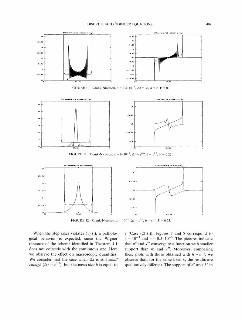
FIGURE 10 Crank-Nicolson, e 0.5.10-3, At 3e, h e, V 0.

density density

FIGURE 11 Crank-Nicolson, e 8.10-3, At c0"6, h c.2, V 0.25.

density density

FIGURE 12 Crank-Nicolson, e 10-3, At e0"6, h e 12, V 0.25.

When the step sizes violates (1) (i), a patholo-gical behavior is expected, since the Wignermeasure of the scheme identified in Theorem 4.1does not coincide with the continuous one. Herewe observe the effect on macroscopic quantities.We consider first the case when At is still smallenough (At e5), but the mesh size h is equal to

e (Case (2) (i)). Figures 7 and 8 correspond toe 10-3 and e 0.5.10-3. The pictures indicatethat n and J converge to a function with smallersupport than n and j0. Moreover, comparingthese plots with those obtained with h e.2, weobserve that, for the same fixed e, the results arequalitatively different. The support of n and J in


density density

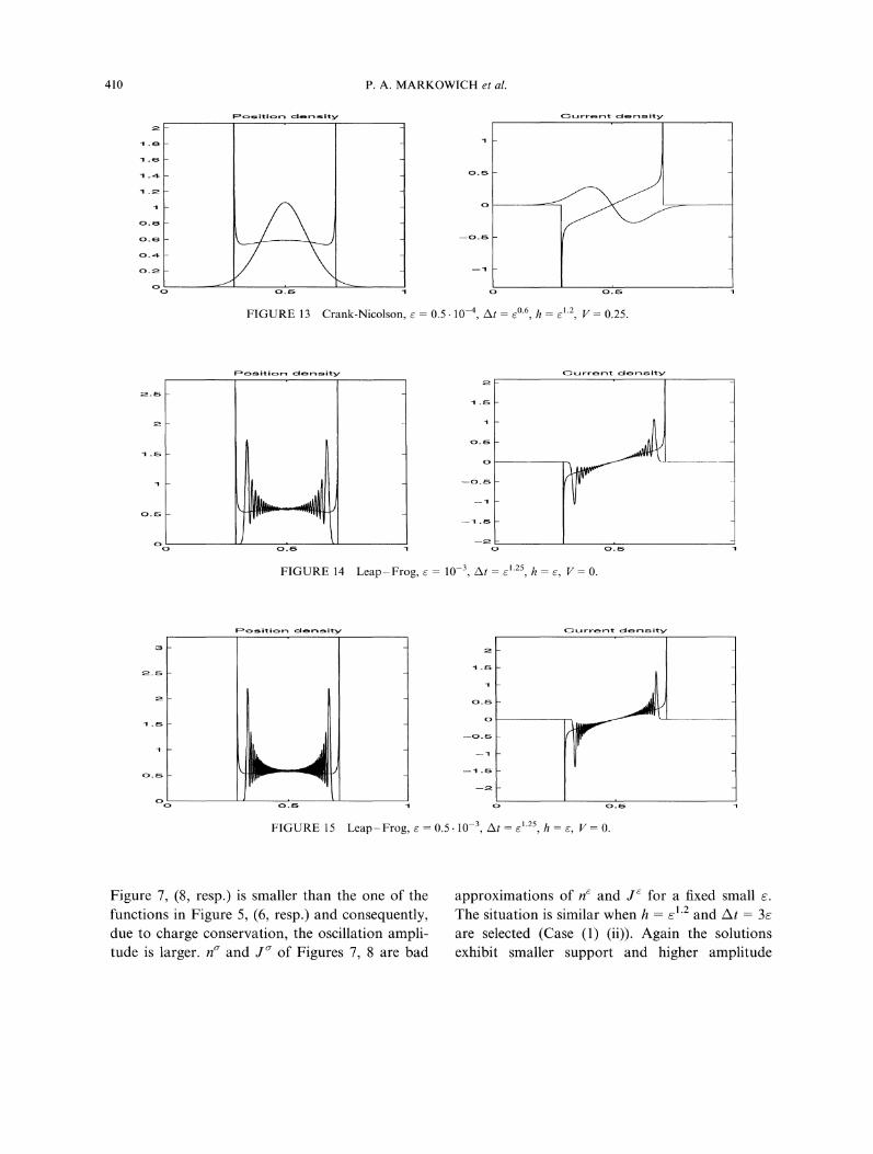
FIGURE 13 Crank-Nicolson, e 0.5.10-4, At 0.6, h .2, V= 0.25.

density density

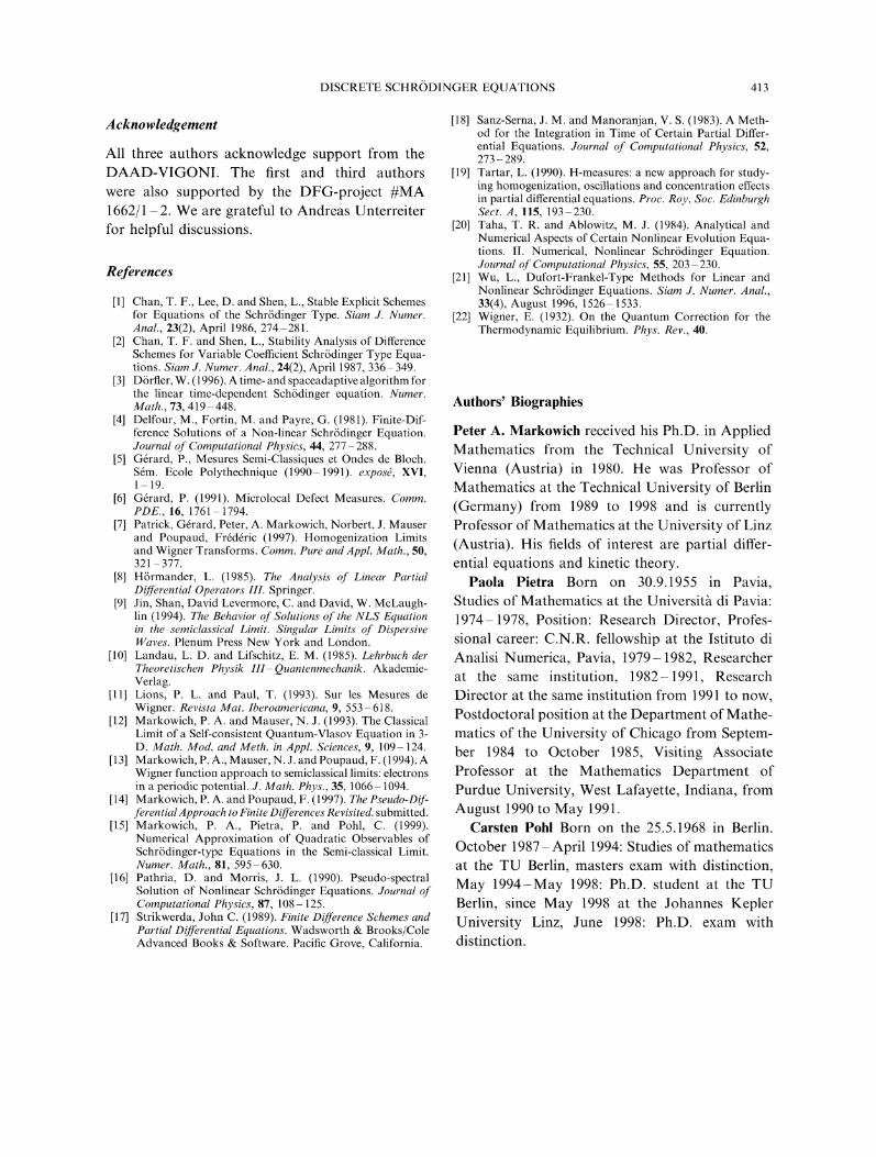
FIGURE 14 Leap-Frog, 10-3, At E1.25, h , V 0.

density density

FIGURE 15 Leap-Frog, e=0.5.10-3 At=25, h=, V =0.

Figure 7, (8, resp.) is smaller than the one of thefunctions in Figure 5, (6, resp.) and consequently,due to charge conservation, the oscillation ampli-tude is larger, n and J of Figures 7, 8 are bad

approximations of n and JC for a fixed small e.The situation is similar when h e 1"2 and At 3eare selected (Case (1) (ii)). Again the solutionsexhibit smaller support and higher amplitude

density density

FIGURE 16 Leap-Frog, e 10-3, At 0.4e, h e, V 0.

Position density density

FIGURE 17 Leap-Frog, e=0.5.10-3, At= 0.4e, h= e, V =0.

1.5

00.1

0 0.2

FIGURE 18 Leap-Frog, e 10-3, At (1/30)e, h e, V 10, 0.2 < x < 0.8, 0 < < 0.1.

0.8


oscillations (see Fig. 9, for e- 0.5.10-3). Theeffect is amplified when both h and At are too

large. Figure 10 illustrates case (2) (ii) with h e,At 3e, for e 0.5.10-3. In order to illustratecase (1) (iii), condition (4.6a) must be fulfilled. Aconstant potential V > 0 is considered, so that Qis bounded away from zero. Figures 11-13 showthe results when V 0.25, h e2, At e6, fora sequence of e’s. When e is large, (the plotfor e 8.10-3 is presented in Fig. 11) it is evidentthat n and J are far away from the correctsolution, but the pictures do not suggest what thelimit of the sequence is. As e becomes smaller, ndoes not exhibit oscillations and its maximumdecreases with e (see Fig. 12) which refers to acomputation with e- 10-3. Figure 13 displays(for e- 0.5.10-4) n and J very close to theinitial value n1 and J:=n(d/dx)Si, in agreementwith the theoretical result W wi.Leap-Frog The Leap-Frog scheme (3.5) has

some interesting properties when being applied toSchr6dinger type equations. It is an explicit scheme,but with a not too restrictive stability condition.For the Schr6dinger equation the sharp stabilitybound is

At h2

< (5e 2 e2 + 0.5Vmaxh 2’

where gma maxx IV(x) I. Moreover, although it isnot a conservative scheme it has similar properties:

’Charge conservation’:

Re (u(x, tn+l)bla(X, tn))dx const

’Energy conservation"

2 Re(VxU(X’tn)VxU(X’tn+l))dx+

V(x)Re (u(x, tn)u(x, tn+l))dx const.

All the tests presented here are carried out with

-u- u, so that z/ w/ (see Theorem 4.2).

Let us discuss case (1) ofTheorem 4.2 first. Only acondition on h is stated, since the stability condition

(5.10) implies that (At/e) goes to zero in this case.For instance, if V 0 is selected, then the stabilitycondition forces (At/e)< 0.5(h2/e2). For h e 1"2

and At 0.49eTM the stability condition is satis-fied and the results for e 2.10-3, e 10-3 e0.5.10-3 are very similar to those of Figures 4-6(obtained with the Crank-Nicolson scheme) andare not reported. Note that in this case the stabilitycondition allows a At very close to At e5 usedin the tests with the Crank-Nicolson scheme. Ofcourse, if h is much smaller than e, (5.10) requires amuch smaller At than the one requested bycondition (i) of Theorem 4.1 for Crank-Nicolson.

All the pathological situations are possible forh O(e). As in the Crank-Nicolson case, when Qpappears in the transport Eq. (4.9) (case (2) (i)), nand J exhibit smaller support and higher oscilla-tions than in the case when the exact Q is present.Figures 14 and 15 show the results for h e,/t e 1"25 with e 10.3 and e 0.5.10-3. Com-paring Figure 15 and Figure 8, which correspondsto case (2) (i) for Crank-Nicolson, no difference isobserved.

In the case (2) (ii), we remark that the term

cd2Q],e in (4.10a), with c At/e, is always posi-tive when the stability condition (5.10) is satisfied.

Figures 16 and 17 show results with e 10-3

and e 0.5.10-3 for At 0.4e, h e and V 0which are very similar to those of Figures 14and 15, since in this case 1- co2g12 is almosth,eInstead, when this coefficient is small, Z and Ware significantly different and they evolve accord-ing to two different laws. The effect on themacroscopic quantities is weird. If, for example,e= 10-3,At=(1/30)e,h=eand V= 10thenthemaximum of n oscillates almost every time step.Figure 18 shows the evolution of n’(x,t) for0_< < 0.1. Although the density n is smooth inthis time intervall (we recall that caustics developat time 0.2) the wave function u (solution ofthe Schr6dinger equation) has oscillations in thephase. A choice of the discretization parametersthat does not take care of this fact can give thewrong results. Actually, Theorems 4.1 and 4.2apply regardless of the occurance of caustics.

DISCRETE SCHRODINGER EQUATIONS 413

Acknowledgement

All three authors acknowledge support from theDAAD-VIGONI. The first and third authorswere also supported by the DFG-project #MA1662/1- 2. We are grateful to Andreas Unterreiterfor helpful discussions.

References

[1] Chan, T. F., Lee, D. and Shen, L., Stable Explicit Schemesfor Equations of the Schr6dinger Type. Siam J. Numer.Anal., 23(2), April 1986, 274-281.

[2] Chan, T. F. and Shen, L., Stability Analysis of DifferenceSchemes for Variable Coefficient Schr6dinger Type Equa-tions. Siam J. Numer. Anal., 24(2), April 1987, 336- 349.

[3] D6rfler, W. (1996). A time- and spaceadaptive algorithm forthe linear time-dependent Sch6dinger equation. Numer.Math., 73, 419-448.

[4] Delfour, M., Fortin, M. and Payre, G. (1981). Finite-Dif-ference Solutions of a Non-linear Schr6dinger Equation.Journal of Computational Physics, 44, 277-288.

[5] G6rard, P., Mesures Semi-Classiques et Ondes de Bloch.Sdm. Ecole Polythechnique (1990-1991). exposd, XVI,1-19.

[6] Gdrard, P. (1991). Microlocal Defect Measures. Comm.PDE., 16, 1761-1794.

[7] Patrick, Gdrard, Peter, A. Markowich, Norbert, J. Mauserand Poupaud, Fr6d6ric (1997). Homogenization Limitsand Wigner Transforms. Comm. Pure and Appl. Math., 50,321-377.

[8] H6rmander, L. (1985). The Analysis of Linear PartialDifferential Operators IlL Springer.

[9] Jin, Shan, David Levermore, C. and David, W. McLaugh-lin (1994). The Behavior of Solutions of the NLS Equationin the semiclassical Limit. Singular Limits of DispersiveWaves. Plenum Press New York and London.

[10] Landau, L. D. and Lifschitz, E. M. (1985). Lehrbuch derTheoretischen Physik III-Quantenmechanik. Akademie-Verlag.

[11] Lions, P. L. and Paul, T. (1993). Sur les Mesures deWigner. Revista Mat. Iberoamericana, 9, 553-618.

[12] Markowich, P. A. and Mauser, N. J. (1993). The ClassicalLimit of a Self-consistent Quantum-Vlasov Equation in 3-D. Math. Mod. and Meth. in Appl. Sciences, 9, 109-124.

[13] Markowich, P. A., Mauser, N. J. and Poupaud, F. (1994). AWigner function approach to semiclassical limits: electronsin a periodic potential. J. Math. Phys., 35, 1066-1094.

14] Markowich, P. A. and Poupaud, F. (1997). The Pseudo-Dif-ferentialApproach to Finite Differences Revisited. submitted.

[15] Markowich, P. A., Pietra, P. and Pohl, C. (1999).Numerical Approximation of Quadratic Observables ofSchr6dinger-type Equations in the Semi-classical Limit.Numer. Math., 81, 595-630.

[16] Pathria, D. and Morris, J. L. (1990). Pseudo-spectralSolution of Nonlinear Schr6dinger Equations. Journal ofComputational Physics, 87, 108-125.

[17] Strikwerda, John C. (1989). Finite Difference Schemes andPartial Differential Equations. Wadsworth & Brooks/ColeAdvanced Books & Software. Pacific Grove, California.

[18] Sanz-Serna, J. M. and Manoranjan, V. S. (1983). A Meth-od for the Integration in Time of Certain Partial Differ-ential Equations. Journal of Computational Physics, 52,273-289.

[19] Tartar, L. (1990). H-measures: a new approach for study-ing homogenization, oscillations and concentration effectsin partial differential equations. Proc. Roy. Soc. EdinburghSect. A, 115, 193-230.

[20] Taha, T. R. and Ablowitz, M. J. (1984). Analytical andNumerical Aspects of Certain Nonlinear Evolution Equa-tions. II. Numerical, Nonlinear Schr6dinger Equation.Journal of Computational Physics, 55, 203-230.

[21] Wu, L., Dufort-Frankel-Type Methods for Linear andNonlinear Schr6dinger Equations. Siam J. Numer. Anal.,33(4), August 1996, 1526-1533.

[22] Wigner, E. (1932). On the Quantum Correction for theThermodynamic Equilibrium. Phys. Rev., 40.

Authors’ Biographies

Peter A. Markowich received his Ph.D. in AppliedMathematics from the Technical University ofVienna (Austria) in 1980. He was Professor ofMathematics at the Technical University of Berlin(Germany) from 1989 to 1998 and is currentlyProfessor of Mathematics at the University of Linz(Austria). His fields of interest are partial differ-ential equations and kinetic theory.

Paola Pietra Born on 30.9.1955 in Pavia,Studies of Mathematics at the Universitt di Pavia:1974-1978, Position: Research Director, Profes-sional career: C.N.R. fellowship at the Istituto diAnalisi Numerica, Pavia, 1979-1982, Researcherat the same institution, 1982-1991, ResearchDirector at the same institution from 1991 to now,Postdoctoral position at the Department of Mathe-matics of the University of Chicago from Septem-ber 1984 to October 1985, Visiting AssociateProfessor at the Mathematics Department ofPurdue University, West Lafayette, Indiana, fromAugust 1990 to May 1991.

Carsten Pohl Born on the 25.5.1968 in Berlin.October 1987-April 1994: Studies of mathematicsat the TU Berlin, masters exam with distinction,May 1994-May 1998: Ph.D. student at the TUBerlin, since May 1998 at the Johannes KeplerUniversity Linz, June 1998: Ph.D. exam withdistinction.

International Journal of

AerospaceEngineeringHindawi Publishing Corporationhttp://www.hindawi.com Volume 2010

RoboticsJournal of

Hindawi Publishing Corporationhttp://www.hindawi.com Volume 2014


Active and Passive Electronic Components

Control Scienceand Engineering

Journal of



RotatingMachinery


Hindawi Publishing Corporation http://www.hindawi.com

Journal ofEngineeringVolume 2014

Submit your manuscripts athttp://www.hindawi.com

VLSI Design



Shock and Vibration


Civil EngineeringAdvances in

Acoustics and VibrationAdvances in



Electrical and Computer Engineering

Journal of

Advances inOptoElectronics

Hindawi Publishing Corporation http://www.hindawi.com

Volume 2014

The Scientific World JournalHindawi Publishing Corporation http://www.hindawi.com Volume 2014

SensorsJournal of


Modelling & Simulation in EngineeringHindawi Publishing Corporation http://www.hindawi.com Volume 2014


Chemical EngineeringInternational Journal of Antennas and

Propagation




Navigation and Observation



DistributedSensor Networks


Semiclassical Analysis of Schr6dinger-type...

Documents

Transcript of Semiclassical Analysis of Schr6dinger-type...