Seeing Through Computation and Artificial Intelligence

Heung‐No Lee, Ph.D.Professor, GIST, KOREA

2016.09.22

1

Agenda Seeing Through Computation 기술과 AI StC 기술 센서지능화 기술

2

강의 요지 및 방향

Seeing through Computation (StC)?

Artificial Intelligence

3

■ 분광기 ■ 레이더

Seeing through Computation (StC) ■ 카메라

빛의성질Ernst Abbe (1840 ~ 1905)

Diffraction Limit

2d

Optical Device

Optical Device

Optical Device

2d

1~10 μm

0.5~5 μm

20~300 nm

0.1 nm

~ 10 μm

VisibleRadioWavelength(meters)

Frequency(Hz)

10

Viruses

BacteriaFrog

Fine DustHumans

Oryong-hall Cell Atoms

Protein

Atomic nucles

3

10 4 10 8 10 12 10 15 10 16 10 18 10 20

10-2

10 -5 10 -8 10 -10 10 -125X10 -6

Infrared Visible Ultraviolet X-ray Gamma RayMicrowave

수학을이용한해상도제고방법

1.01.0

1.0 1.0 1.01.0 1.0 1.0

1.0

0 0 0 00 0 0 0 0

0 0 00 0 0

0 0 0 00 0 01.0

=

= y I x

0.8 0.10.8 0.8 0.10.1 0.8 0.8 0.1

0.1 0.8 0.8 0.10.1 0.8 0.1 0.8

0.1 0.8 0.1

0.1 1.0 00.9 1.0 01.8 1.0 1.01.8 1.0 1.00.9 00.1 0

=

1 = y A x

12

1

1

min s. t. =

T T

x y Ax

x A A A y

Interference free Interfered optics

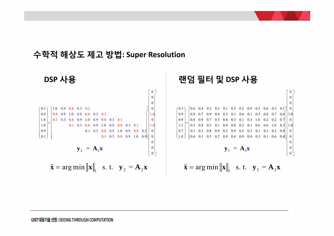
수학적 해상도 제고 방법: Super Resolution

0.8 0.10.1

0.1 0.8 0.8 0.0.8 0.8 1.0

0.1 0.8

0.9 0.30.9 0.9 0.30.3 0.9 0.9 0.3

0.3 0.9 0.9 0.30.3 0.

000

0.1 1.0 00.9 1.0

10.8 0.1

0.8 0.80.1

1.8 1.0 01.8 1.00.9 0.1 1.00.1

1

0.9 0.9 0.3

0.3 0 1.. 0098 .9

.000000

2 21arg min s. t. = x x y A x

0.3 0.6 0.4 0.2 0.3 0.1 0.5 0.2 0.9 0.2 0.6 0.3 0.10.9 0.9 0.7 0.9 0.4 0.3 0.1 0.6 0.1 0.5 0.6 0.7 0.60.9 0.8 0.9 0.7 0.5 0.8 0.3 0.1 0.3 1.0 0.2 0.2 0.71.2 0.3 0.8 0.3 0.1 0.9 0.8 0.3 0.1 0.6 0.6 1.0 0.30.7 0.1 0.3 0.8 0.9 0.2 0.1.8

0000

1.00

1.09 0.5 0.3 0.1 0.1 0.3 0.9 0

0.6 0.1 0.3 0.2 0.9 0.4 0.9 0.8 0.3 0.1 0.6 0.4 0000

3 31arg min s. t. = x x y A x

2 2 = y A x 3 3 = y A x

DSP 사용 랜덤 필터 및 DSP 사용

최근4년간성과

Artificial Intelligence

지능이란?‐ 주어진 상황을 인지하고 목표를 효과적으로 달성하는 결정, 임무 수행 (한정된 자원하에) 

Machine learning– Supervised Learning– Unsupervised Learning– Reinforcement Learning (RL)– Deep Neural Network

9

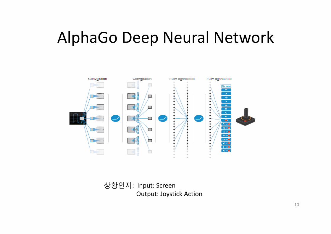
AlphaGo Deep Neural Network

10

상황인지:  Input: ScreenOutput: Joystick Action

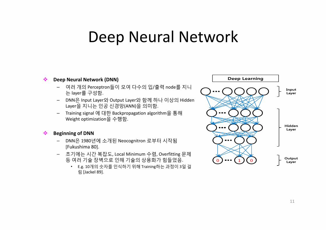
Deep Neural Network

Deep Neural Network (DNN)– 여러 개의 Perceptron들이 모여 다수의 입/출력 node를 지니

는 layer를 구성함.– DNN은 Input Layer와 Output Layer와 함께 하나 이상의 Hidden 

Layer을 지니는 인공 신경망(ANN)을 의미함.– Training signal 에 대한 Backpropagation algorithm을 통해

Weight optimization을 수행함.

Beginning of DNN– DNN은 1980년에 소개된 Neocognitron 로부터 시작됨

[Fukushima 80].– 초기에는 시간 복잡도, Local Minimum 수렴, Overfitting 문제

등 여러 기술 장벽으로 인해 기술의 상용화가 힘들었음. • E.g. 10개의 숫자를 인식하기 위해 Training하는 과정이 3일 걸

림 [Jackel 89].

11

AlphaGo Tree Search

12

AlphaGo

Tree Search  Supervised (human 

players), Reinforced learning (Self‐play 학습)

Trim the possibilities with Deep Neural Network (총action의 가지 수를 줄임)

Breadth Search Depth Search Aim to make the best 

decision among sequences of actions, rather than single actions

13

RL 및 기보 학습의 결과

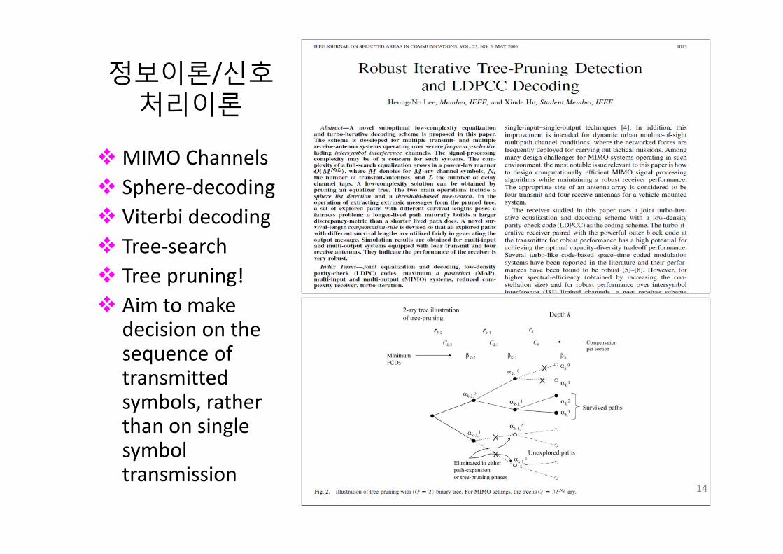
정보이론/신호처리이론

MIMO Channels Sphere‐decoding Viterbi decoding Tree‐search Tree pruning! Aim to make 

decision on the sequence of transmitted symbols, rather than on single symbol transmission  

14

Seeing Through Computation기술은

눈, 코, 귀, 촉각, 뇌파 등을 측정하는 센서를 DSP기술을 통해 그 성능을 향상 시키는 것에 초점을 맟추어왔읍니다.

최근 인공지능의 발전은, 시스템을 한 번에 최적화하려 하기 보다는, 스스로 학습할 수 있게 만들어 스스로 상황에 맟추어 개선할 수 있게 만드는 것이 더좋다는 것을 시사 합니다.

이에, 센서가 스스로 학습을 통하여 성능을 개선 시키는 시스템으로 StC기술을 개발 하고자 목표 합니다. 

15

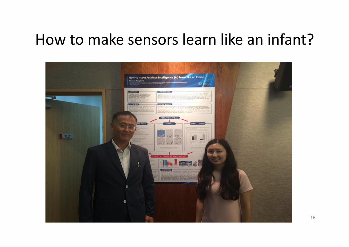
How to make sensors learn like an infant?

16

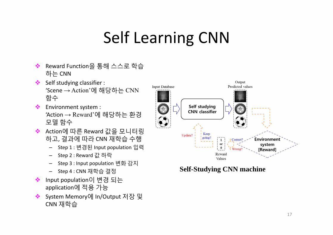
Self Learning CNN Reward Function을 통해 스스로 학습

하는 CNN Self studying classifier : 

‘Scene → Action’에 해당하는 CNN 함수

Environment system : ‘Action → Reward’에 해당하는 환경모델 함수

Action에 따른 Reward 값을 모니터링하고, 결과에 따라 CNN 재학습 수행

– Step 1 : 변경된 Input population 입력– Step 2 : Reward 값 하락– Step 3 : Input population 변화 감지– Step 4 : CNN 재학습 결정

Input population이 변경 되는application에 적용 가능

System Memory에 In/Output 저장 및CNN 재학습

17

Self-Studying CNN machine

Self Learning CNN

18

Input Output Reward Optimized Weight

1

1

‐1

→

1

1

Input Population

<Phase 1>

12

12

<Phase 2>

12

14

14

Expected Reward values (Calculation)

Re

12 1

12 1 1

Re

12 1

14 1

14 1

12

Focus Areas in this talk

19

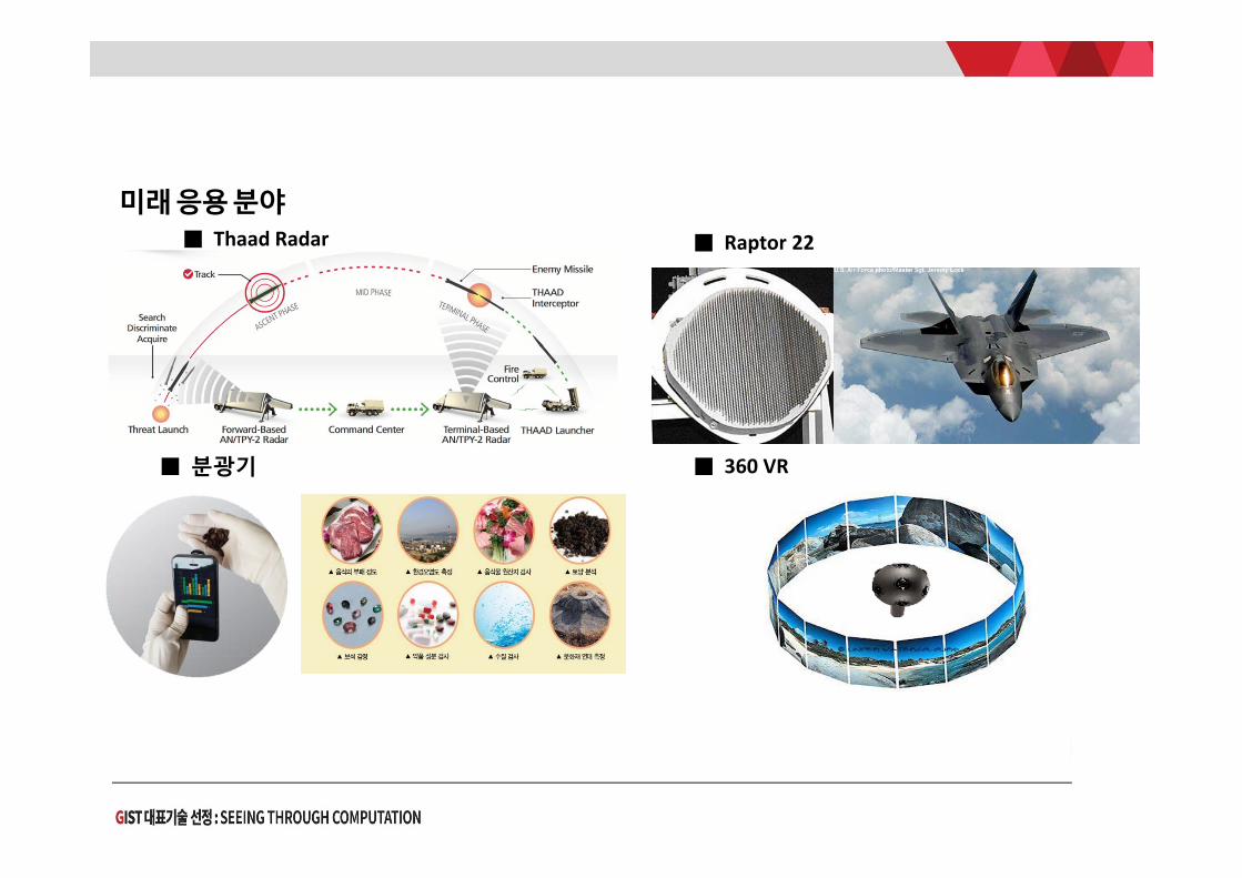
■ 분광기 ■ 360 VR

미래응용분야■ Raptor 22■ Thaad Radar

Compressed sensing (CS) – New signal acquisition techniques [Donoho06], 

cited >4000 times.

– MIT 2007 Tech Review, “Top 10 Emerging Technologies”

CS is to find sparse solution from an under‐determined linear system.

– Real, complex field

Many application areas: Cameras, Medical Scanners, ADCs, Radars, …

22

Background

MyM NF

Nx

1ˆ arg min subject to

xx x F x y

y Fx=

M N

Have you seen this before?

We can draw a graph for y = Fx, shown above.  Yes!!! Channel codes—Syndrome decoding!

Two applications:– Compressed measurement y and recovery of uncompressed data x– Super‐resolution of hidden x from limited measurement y

+ + + + + +

y1 y2 y3 y4 y5 y6

x1 x2 x3 x4 x5 x6 x7 x8 x9 x10 x11 x12

전세계적 연구 동향 (압축센싱이란) 2006년 정보이론과 신호처리 분야에 소개된 압축센싱이론은

응용 측면에서 한 마디로 요약하면 ‘영상 및 음성 등의 자연신호를 압축적으로센싱(Encoding) 할 수 있으며, 그렇게 했을 때 적은 량의 측정샘플 만으로도 신호를 복원(Decoding)할 수 있다’ 정도로 표현 할 수 있음. – 2008 Rice대학 Single‐Pixel Camera, 단 한 개의 포토센서로 영상을 압축하고

복원할 수 있음 시연하고 이론의 실제성 입증.

압축적 샘플링(Encoding)과 신호 복원(Decoding) 문제는 하나의 간단한 연립방정식 y = Ax 으로 표현 가능함. – A ~ M x N 측정행렬이라 칭함. – M<N 일 때 압축이 일어남. 

신호복원은 측정행렬 A를 알고 있는 상황에서, y 로부터 x를 찾아내는, 즉 역문제를 푸는 문제임.

이 역문제가 잘 풀리는 경우는? 24

혁신 기술 출현 (혁신기술 출현) 압축센싱은 또한 “적은 수의 센서로도” 혹은

“짧은 시간 동안의 측정으로도” 신호를 높은 해상도로 복원하는데에도 응용 가능함이 밝혀졌음.

레이더, fMRI, 현미경등 영상장치들은 신호가 센서에 도달하기까지 어떻게 변화하는지를 나타내는 광물리학적 전달 함수가 잘 알려져 있는데, 이 점을 사용하여 Decoding에 필요한측정행렬 A를 만들어내고, Diffraction Limit등을 돌파하는 초고해상도 신호복원이 가능함이 알려짐.

이런 응용연구 결과의 발표는, 2010년 전후로부터 현재까지지속적으로 이루어지고 있으며, 초 고해상도 레이더, 초 광대역 신호 측정, 촬영시간이 크게 단축된 fMRI 머신, 초 고해상도 현미경 등의 혁신 기술의 출현을 가능케 하고 있음.

25

Sparse Representation 압축센싱분야에서 개발된 Decoder 알고리즘은 또한 신호를 희소하게

표현 하는 방법 (Sparse Representation) 으로도 응용되어 왔음. 

즉, 신호의 고유정보를 잃지 않고 신호의 Dimensionality를 크게Reduction 하는 방법으로 쓰이고 있음.

나아가, 신호를 알려진 몇 가지의 클래스로 구분하는데 뛰어난 성능을보임이 보고됨. 

CCTV 카메라에 찍힌 사람의 이상 행동 양식 구분, 사람의 얼굴 검색 등Big Data 처리 및 분석 등에도 Sparse Representation Classification이라는이름으로 응용되고 있음. 

한 예로, 사용자의 뇌파 신호를 구분하여 컴퓨터 명령을 내릴 수 있는Brain‐Computer Interface 용 분류알고리즘을 들 수 있음.

26

Encoding 연구의 혁신성압축센싱의 Encoding 문제는 아날로그 신호 x(t)를 아날

로그 도메인 상에서 압축적으로 샘플링하여 디지털 샘플 벡터 y를 얻는 전기/전자/재료 공학적 장치를 만들어내야하는 문제임. 

다시 말해, 압축센싱이론 논문에서 흔히 다루는, 이미 디지털 샘플링이 완료된 신호 벡터 x를 측정행렬 A와 곱하여 y를 얻는 것은 Encoding 문제가 아님. 

아날로그 도메인에서 연속적인 신호 x(t)를 랜덤한 반응패턴을 가진 함수와 곱하고, 그 결과를 더해서 샘플을 취하는 장치를 만드는 연구 및 실제 구현이 혁신적 성과를내기 위해 꼭 필요함. 

27

Decoding 연구 지속의 중요성

많은 Decoder가 현재 개발 되었음– Gaussian, FFT, Bernoulli 센싱등 문제가 수학적으

로 잘 알려진 형태 일 때

특정 문제에 특화된 Decoder 개발 필요 함– Photonics, Spectrometers, Electronic Eyes, …– Non negative signal sensing– No general sensing matrices

28

Compressive Spectrometers for Super Resolution

State‐of‐the art portable spectrometers

Spectrometer: Used to find the spectrum of an optical signal

It takes in the light, breaks it into its spectral components, and displays them in a portable device such as smart phones.

The ability of the spectrometer in revealing fine information is determined by its “Resolution”

Problem: Resolution is limited by the number of filters

Air quality monitoring in oil spillsAir quality monitoring in oil spills Biomedical DNA detectionBiomedical DNA detection

Applications

Analysis of Behavior of ChemicalsAnalysis of Behavior of Chemicals

29

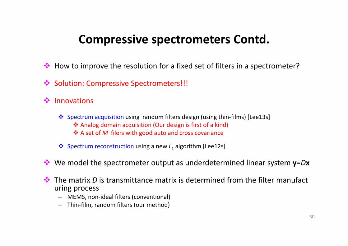
Compressive spectrometers Contd.

How to improve the resolution for a fixed set of filters in a spectrometer?

Solution: Compressive Spectrometers!!! 

Innovations

Spectrum acquisition using  random filters design (using thin‐films) [Lee13s] Analog domain acquisition (Our design is first of a kind) A set of M filers with good auto and cross covariance

Spectrum reconstruction using a new L1 algorithm [Lee12s]

We model the spectrometer output as underdetermined linear system y=Dx

The matrix D is transmittance matrix is determined from the filter manufacturing process 

– MEMS, non‐ideal filters (conventional)– Thin‐film, random filters (our method)

30

Various Transmittance Functions

31

300 400 500 600 7000

0.5

1

Wavelength (nm)

Tra

nsm

ittan

ce

300 400 500 600 7000

0.5

1

Wavelength (nm)

Tra

nsm

ittan

ce

300 400 500 600 7000

0.5

1

Wavelength (nm)(a)

Tra

nsm

ittan

ce

StopbandPassband

Filter − 5

Filter − 20

Filter − 34

300 350 400 450 500 550 600 650 7000

0.5

1

Wavelength (nm)

Tra

nsm

ittan

ce

300 350 400 450 500 550 600 650 7000

0.5

1

Wavelength (nm)

Tra

nsm

ittan

ce

300 350 400 450 500 550 600 650 7000

0.5

1

Wavelength (nm)(b)

Tra

nsm

ittan

ce

Filter − 5

Filter − 20

Filter − 34

300 350 400 450 500 550 600 650 7000

0.5

1

Wavelength (nm)

Tra

nsm

ittance

300 350 400 450 500 550 600 650 7000

0.5

1

Wavelength (nm)

Tra

nsm

ittance

300 350 400 450 500 550 600 650 7000

0.5

1

Wavelength (nm)(a)

Tra

nsm

ittance Filter−34

Filter−20

Filter−5

Conventional Design

1. Stringent filter design

2. Local sampling

Our approach

1. Ease of filter design 

2. Holistic sampling

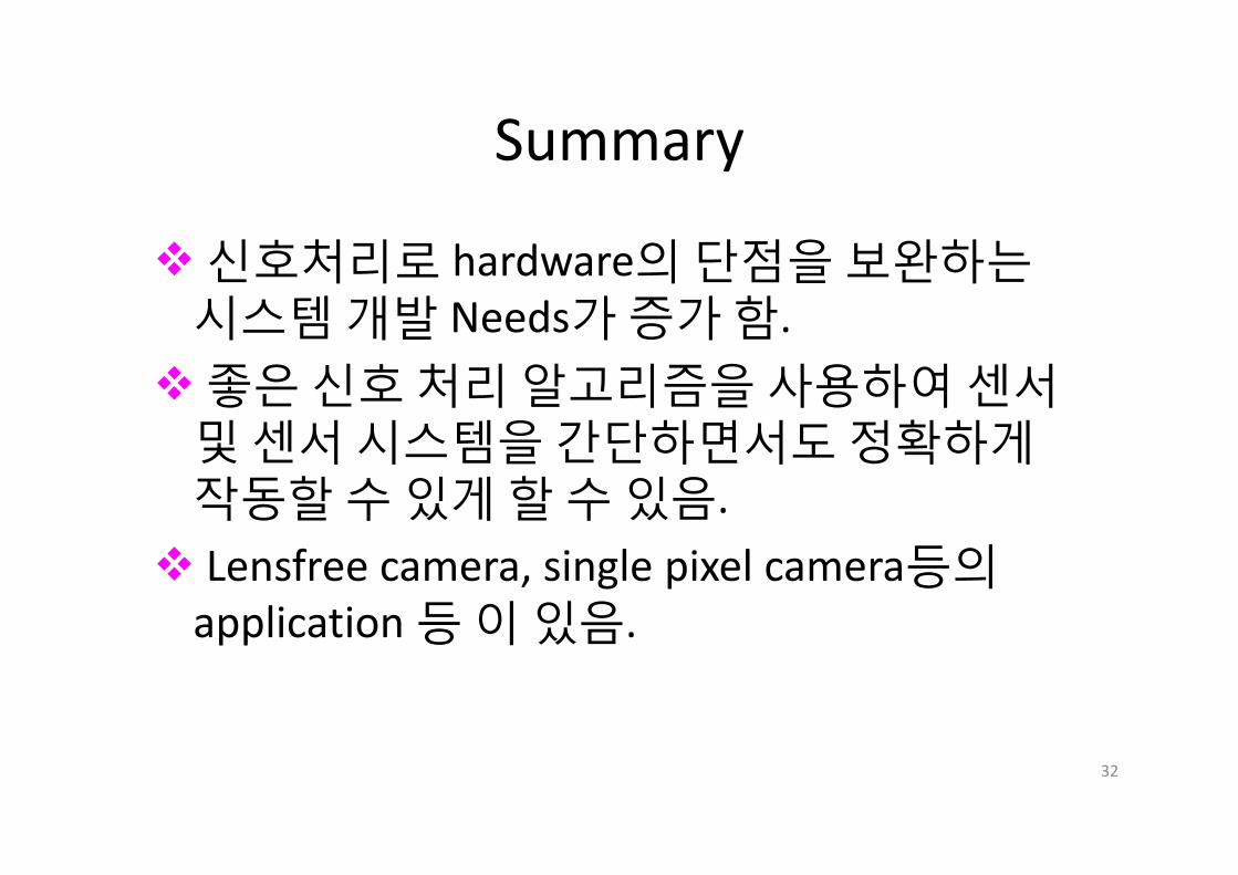
Summary

신호처리로 hardware의 단점을 보완하는시스템 개발 Needs가 증가 함.좋은 신호 처리 알고리즘을 사용하여 센서

및 센서 시스템을 간단하면서도 정확하게작동할 수 있게 할 수 있음. Lensfree camera, single pixel camera등의application 등 이 있음.

32

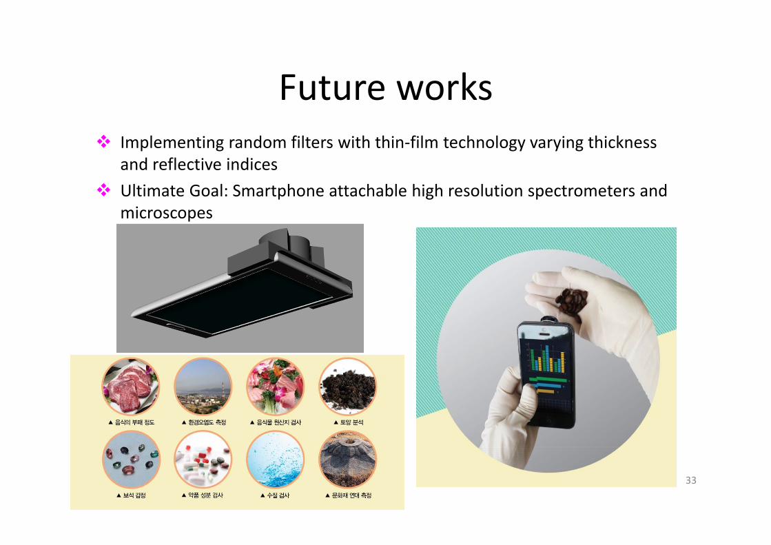
Future works Implementing random filters with thin‐film technology varying thickness 

and reflective indices Ultimate Goal: Smartphone attachable high resolution spectrometers and

microscopes

33

COMPutational Compound EYE (COMP‐EYE) imaging system

34

Hemispherical Apposition Compound Eyes

Implemented by stretchable microlens array and photodiodes

Limitation: 180 pixels (16x16 photo diodes)

35

Computational Compound EYE imaging system Eyes in nature

– Camera-type eye vs. Compound eye

Due to diffraction limit and low density of photoreceptors, the resolution of compound eyes is limited.

36

- Single lens system- High resolution- Pattern recognition

- Multi-lens system- Wide field of view (FOV),

Infinite depth of field (DOF)- Motion detection

Camera-type Eye Compound Eye

Computational Compound EYE imaging system COMP-EYE

– We aim to improve the resolution of the compound eye imaging system by designing larger acceptance angles of ommatidia and using a digital signal processing (DSP) technique

– Larger acceptance angles enable each ommatidium to observe multiple pieces of information all at once.

– Each piece of information is observed multiple times by multiple ommatida each with different perspectives.

– By exploiting this, the DSP technique recovers the object image with high resolution.

37

Conventional System Computational Compound Eye

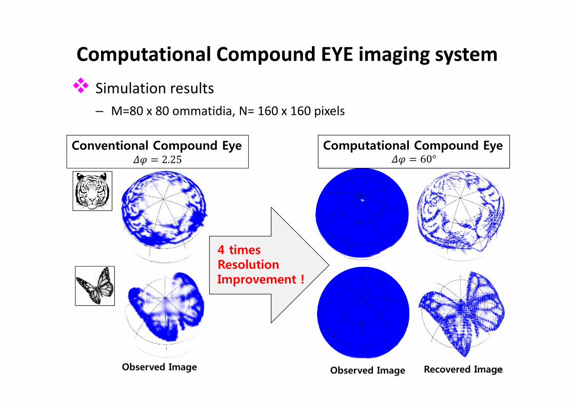
Computational Compound EYE imaging system Simulation results

– M=80 x 80 ommatidia, N= 160 x 160 pixels

38

Conventional Compound Eye2.25

Recovered Image

Computational Compound Eye60°

Observed ImageObserved Image

4 timesResolution Improvement !

3D 영상센서와 초소형 라이다(LiDAR)를 결합한차세대 3D인식 복합센서모듈 기술개발

• 최종 연구 목표 차세대 3D 인식 복합센서 및 장애물 충돌 회피 알고리즘 개발

3D 광영상 센서와 초소형 LiDAR를결합한 복합센서 개발• 3 Lows: 무게, 부피, 소비전력

복합영상처리 알고리즘 및 최적 경로결정 알고리즘 개발• 탑재 가능 영상/신호 처리 알고리즘

장애물 충돌회피 알고리즘 개발 소형 드론 테스트베드 개발

39

복합영상센서 개요

60o

20o

측정 거리

광각(FOV*)

3D 광센서

MEMS LiDAR

*Field of view

두 가지 센서 융합하여장단점을 상호보완 !!

40

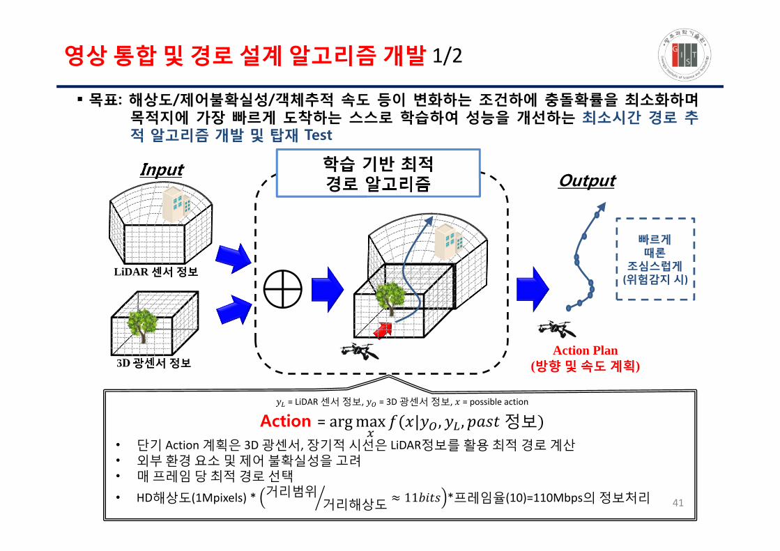
목표: 해상도/제어불확실성/객체추적 속도 등이 변화하는 조건하에 충돌확률을 최소화하며목적지에 가장 빠르게 도착하는 스스로 학습하여 성능을 개선하는 최소시간 경로 추적 알고리즘 개발 및 탑재 Test

= LiDAR 센서 정보,  = 3D 광센서 정보, = possible action

Action = argmax | , , 정보• 단기 Action 계획은 3D 광센서, 장기적 시선은 LiDAR정보를 활용 최적 경로 계산• 외부 환경 요소 및 제어 불확실성을 고려• 매 프레임 당 최적 경로 선택

• HD해상도(1Mpixels) *  거리범위거리해상도 11 *프레임율(10)=110Mbps의 정보처리

영상 통합 및 경로 설계 알고리즘 개발 1/2

학습 기반 최적경로 알고리즘 Output

Action Plan(방향 및 속도 계획)

Input

3D 광센서 정보

LiDAR 센서 정보

빠르게때론

조심스럽게(위험감지 시) 

41

Tree Search 주행 경로 탐색 알고리즘

Tree search 문제 모델링• 위치( ), 동작( ), 충돌 확률( )

Breadth 감소 방법 개발 (3D 광센서)• 가능한 동작 제한 → Breadth 복잡도 감소

Depth 감소 방법 개발 (MEMS LiDAR)• 충돌 확률 Regression → Depth 복잡도 감소

영상 통합 및 경로 설계 알고리즘 개발 2/2

D

근거리Tree

searching

충돌 원거리Regression

t=1

t=0

t=2

t=10

1 2 4 8 5

884

8

충돌

제한된 컴퓨팅 자원 및 외부 방해 요소 하에서경로안정성 유지

Reinforcement Learning (RL)

주행 경로 탐색 알고리즘 upgrade

SERVER

무인 이동체 운용

알고리즘탑재

운용데이터및 결과

주행 경로 탐색 알고리즘 예제 Tree search 예제

42