RIT “Stochastic Dynamics:

Models, Analysis and Numerics”

Lecture 2: Problems and challenges in stochastic dynamics

Maria Cameron

Why do we use the Brownian Motion?

dxj =pjmj

dt

dpj = (−∇V (x) − γmj−1pj )dt + 2β−1γ dwj ,

j = 1...M N

dxidt

=pimi

dpidt

= −∇V (x)

i = 1...N

Two main effects:- slowing down

-random change of the direction of motion

Alanine-Dipeptide in the water(by Maddalena Venturoli (U. Rome, Italy))

Are there other mathematically-tractable

options?Gaussian Process with Correlation in time

Levy Flights

Difference of two Poisson processes

A process with heavy tails (e.g. with Student’s pdf)

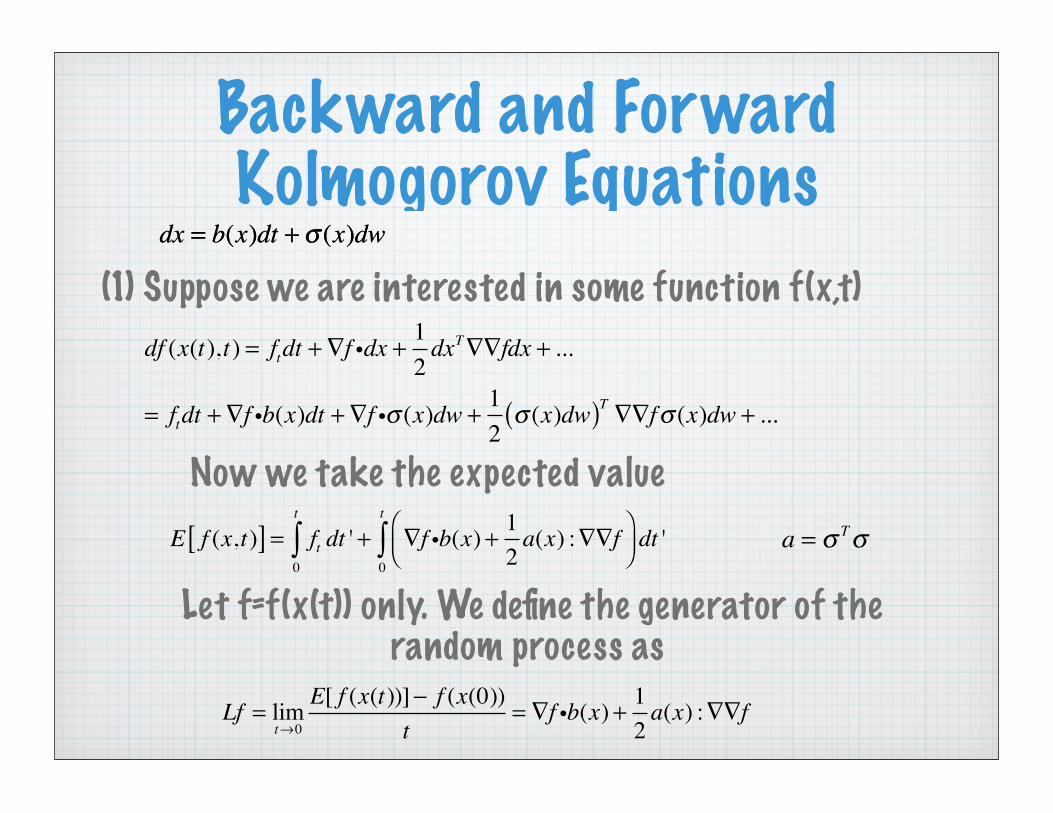
Backward and Forward Kolmogorov Equations

dx = b(x)dt +σ (x)dw

(1) Suppose we are interested in some function f(x,t)

df (x(t),t) = ftdt +∇f idx +12dxT∇∇fdx + ...

= ftdt +∇f ib(x)dt +∇f iσ (x)dw +12

σ (x)dw( )T ∇∇fσ (x)dw + ...

Now we take the expected value

E f (x,t)[ ] = ft dt '0

t

∫ + ∇f ib(x) + 12a(x) :∇∇f⎛

⎝⎜⎞⎠⎟dt '

0

t

∫

Let f=f(x(t)) only. We define the generator of the random process as

Lf = limt→0

E[ f (x(t))]− f (x(0))t

= ∇f ib(x) + 12a(x) :∇∇f

a = σ Tσ

dx = b(x)dt +σ (x)dw

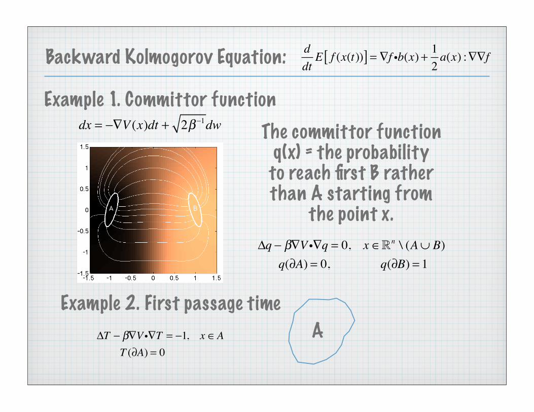
Example 1. Committor functiondx = −∇V (x)dt + 2β−1dw The committor function

q(x) = the probabilityto reach first B rather than A starting from

the point x.

Δq − β∇V i∇q = 0, x ∈n \ (A∪ B)q(∂A) = 0, q(∂B) = 1

Example 2. First passage time

ΔT − β∇V i∇T = −1, x ∈AT (∂A) = 0

A

Backward Kolmogorov Equation:

ddtE f (x(t))[ ] = ∇f ib(x) + 1

2a(x) :∇∇f

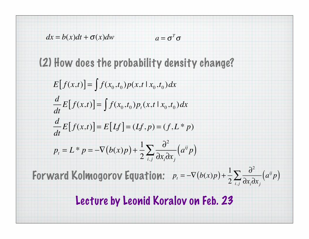
(2) How does the probability density change?

E f (x,t)[ ] = f (x0 ,t0 )p(x,t | x0 ,t0 )dx∫ddtE f (x,t)[ ] = f (x0 ,t0 )pt (x,t | x0 ,t0 )dx∫

ddtE f (x,t)[ ] = E Lf[ ] = (Lf , p) = ( f ,L * p)

pt = L * p = −∇ b(x)p( ) + 12

∂2

∂xi∂x ji, j∑ aij p( )

a = σ Tσdx = b(x)dt +σ (x)dw

Forward Kolmogorov Equation: pt = −∇ b(x)p( ) + 12

∂2

∂xi∂x ji, j∑ aij p( )

Lecture by Leonid Koralov on Feb. 23

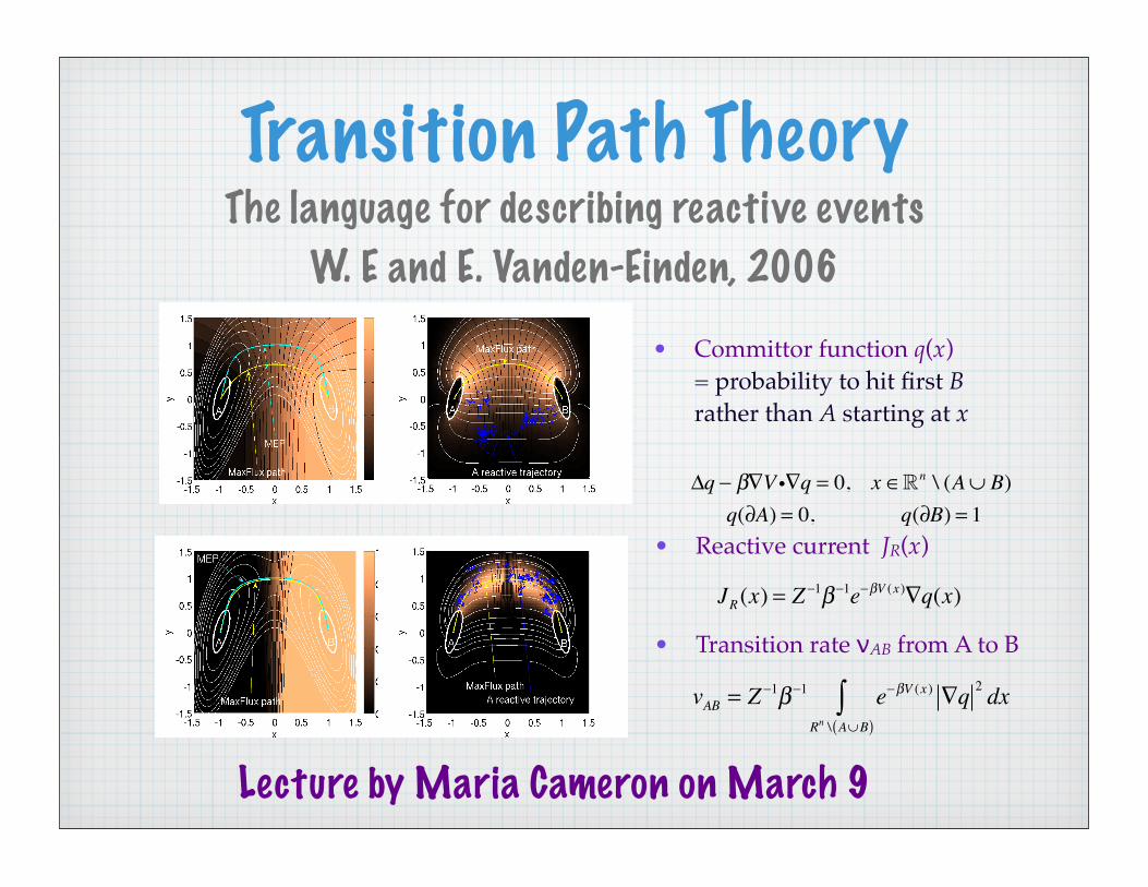
Transition Path TheoryThe language for describing reactive events

W. E and E. Vanden-Einden, 2006

• Committor function q(x) = probability to hit first B rather than A starting at x

Δq − β∇V i∇q = 0, x ∈n \ (A∪ B)q(∂A) = 0, q(∂B) = 1

• Reactive current JR(x)

JR (x) = Z−1β−1e−βV (x )∇q(x)

vAB = Z−1β−1 e−βV (x ) ∇q 2 dx

Rn \ A∪B( )∫

• Transition rate νAB from A to B

Lecture by Maria Cameron on March 9

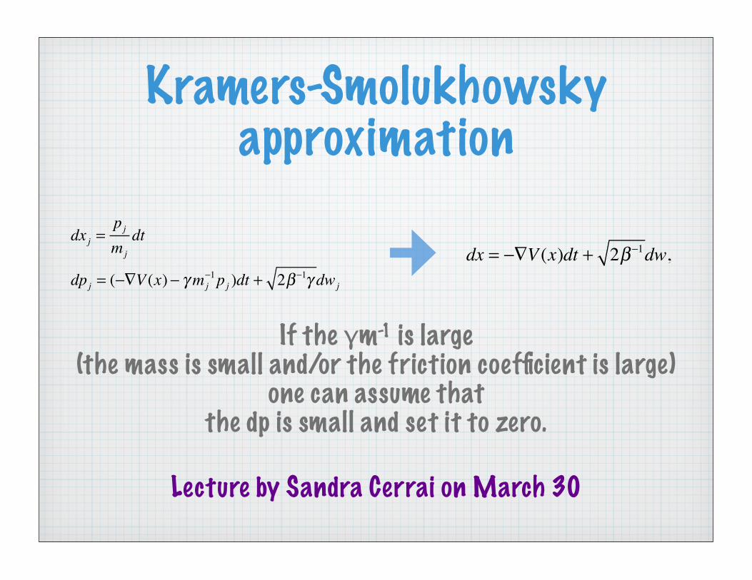
Kramers-Smolukhowsky approximation

dx = −∇V (x)dt + 2β−1dw,

If the γm-1 is large (the mass is small and/or the friction coefficient is large)

one can assume that the dp is small and set it to zero.

Lecture by Sandra Cerrai on March 30

dxj =pjmj

dt

dpj = (−∇V (x) − γmj−1pj )dt + 2β−1γ dwj

Illustration on theDouble-Well potential V(x)=x4-2x2

β=∞β=10γ=1

β=10γ=3

dxj = vjdt

dvj = (−∇V (x) − γmj−1vj )dt + 2β−1γmj

−1dwj

What if mass and/or temperature are not small ?

β=1 γ=1

β=3 γ=1

β=1 γ=0.3

β=3 γ=0.3

β=10 γ=0.3

Difficulty

We can solve the Backward and Forward Kolmogorov Equations only if

the dimension of the phase space is low

the entries of the matrix preceding dw are not too small

Another approach: direct simulations

Monte-Carlo(1) Propose a move.

E.g. pick a spin and flip it.

(2) Calculate the quantity

e-βH(new state)/e -βH(old state) = e -β∆H

(3) if e -β∆H > 1 do the proposed moveotherwise do it with probability e -β∆H

and remain in the old state with probability 1 - e -β∆H.

Monte-Carlo allows to calculate average values using the ergodicity. Important feature: One does not need to know the normalization constant for the pdf.

Problems: (1) There can be high rate of rejectance of the proposed states(2) Equilibration might not happen for very long time due to correlation

Lecture by Jonathan Weare (U. Chicago) on April 6

2D Ising model

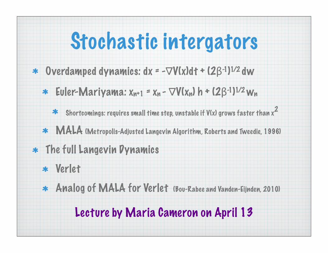
Stochastic intergatorsOverdamped dynamics: dx = -∇V(x)dt + (2β-1)1/2 dw

Euler-Mariyama: xn+1 = xn - ∇V(xn) h + (2β-1)1/2 wn

Shortcomings: requires small time step, unstable if V(x) grows faster than x2

MALA (Metropolis-Adjusted Langevin Algorithm, Roberts and Tweedie, 1996)

The full Langevin Dynamics

Verlet

Analog of MALA for Verlet (Bou-Rabee and Vanden-Eijnden, 2010)

Lecture by Maria Cameron on April 13

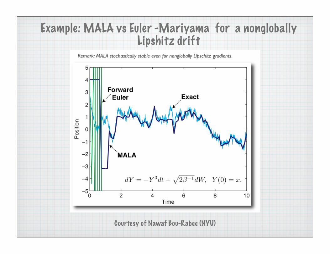
Courtesy of Nawaf Bou-Rabee (NYU)

Example: MALA vs Euler -Mariyama for a nonglobally Lipshitz drift

Analytical tools for the case of small

noise

Large Deviation Theory

• SDE

• F.-W. action functional

• Transition probability along the path

• If two minima are separated by a single mountain pass then the path that satisfies is the MEP, and the minimum is achieved in the limit of infinite time

Freidlin and Wentzell, 1979, 1998

dx = −∇V (x)dt + 2β−1dw

ST (ϕ) = ϕ t +∇V (ϕ(t)) 2 dt0

T

∫∝ e−βST

minT ,ϕ (t )

ST (ϕ )

Lecture by Sandra Cerrai on March 2

Methods for finding transitions paths

• Methods for computing transition paths at zero temperature limit:

• String method (E, Ren and V.-E., 2002)

• Nudged elastic band method (Jonsson et al, 1998)

• MaxFlux functional (Cameron and V.-E., 2010)

• Methods for finding saddle points:

• Dimer method (Henkelman and Jonsson, 1999)

• Activation-relaxation technique (Barkema, Mousseau, 2001 )

• Methods for computing rare events at finite temperature:

• Finite temperature string method (E, Ren and V.-E., 2005)

• MaxFlux Functional (Berkowitz, 1983; Huo and Straub, 1997)

Lecture by Maria Cameron

on March 16

Challengies

High dimensionality of the phase space

Complex and expensive-to-evaluate potential

Multiple transition paths

Example. LJ38

V = 4 rij−12 − rij

−6( )i< j∑

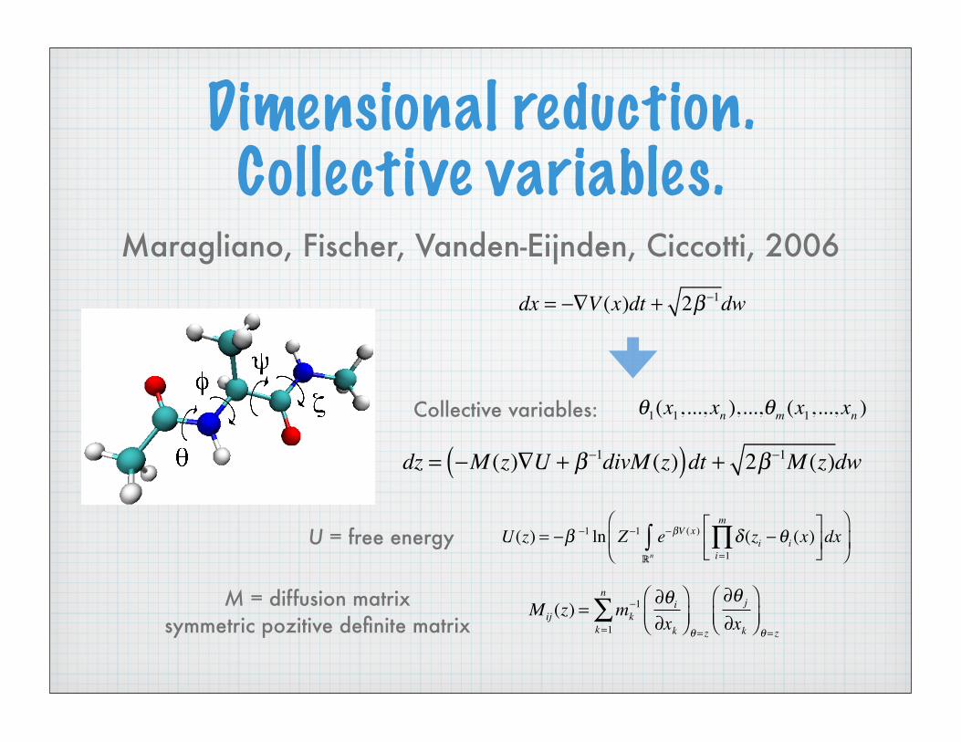
Dimensional reduction.Collective variables.

dx = −∇V (x)dt + 2β−1dw

dz = −M (z)∇U + β−1divM (z)( )dt + 2β−1M (z)dw

M = diffusion matrixsymmetric pozitive definite matrix

Maragliano, Fischer, Vanden-Eijnden, Ciccotti, 2006

Mij (z) = mk−1 ∂θi

∂xk

⎛⎝⎜

⎞⎠⎟k=1

n

∑θ= z

∂θ j

∂xk

⎛⎝⎜

⎞⎠⎟θ= z

θ1(x1,..., xn ),...,θm (x1,..., xn )Collective variables:

U(z) = −β −1 ln Z −1 e−βV (x ) δ (zi −θi (x)

i=1

m

∏⎡⎣⎢

⎤⎦⎥dx

Rn∫

⎛

⎝⎜

⎞

⎠⎟U = free energy

April 20. Dionisios MargetisProblems in materials science:

Interfaces and crystal surfaces

April 20. Dionisios MargetisA taste of mathematical physics:

Mori-Zvanzig formalism