RADAR PRINCIPLES

I Introduction

Radar is a general technique, willcli has a wide range of \, ariability depending o11 the type

of targets to be measured. A radar can be designed to IlTeasure a bullet, \\, bile another

may observe a planet. The radio frequency spectrum employed also spreads out overinariv decades.

The target of radars described here is the earth's atmosphere. Ivlore precisely, it

is so called clear air echoes from the earth's atmosphere produced by fluctuations of

atmospheric index of refraction. we will refer this kind of radar as the atmospheric radar

here. There is also a catego^, of radar' called weather radar, \vincli observes precipitation

as its principal target. Althougli much is common, in principle, to the weather radar andthe atmospheric radar, \\, e do not discuss the former here. Those who are interested in

weather radars are referred to standard text books such as Battan (1973) or Doviak and

Z", IC (1984).

It is possible for powerful weather radars to observe the clear-air echoes. Actually,

the name clear-air echo is given in the history of development of the weather radar to

classify echoes fron} unknown targets. Above mentioned text books also discuss about

the clear-air echoes in some details, but the major difference between their approacli and

ours is simply that we discuss radars specially designed to observe the clear-air echoes.

As we will see later, this difference affects the choice of frequency, requirement on the

sensitivity, and the way data are processed. As a consequence, these two types of radars

often look surprisingIy different.

\\'eather radar usually use frequencies of SHF ba. rid (3-30 GHz), while atmospheric

rodars make use of mad" lower HF (3-30 Min), VHF (30-300 Min), or UHF (300 Min-

3 GHz) bands. Antenna size of weather radarsis a few to about ten metersin diameter, but

an} atmospheric radar in^, require a diameter of more than a hundred meters, depending

Radio Atmospheric Science Center

Kyoto University, Uji, 1<yot0 6/1, Japan

Torn Sato

"

"

2-I

on its target region. Operational atmospheric radars have antennas witli dialneter of 10-300 in. Weather radars cover a wide horizontal area of TIP to several hundred kilometers in

radius by scanning their antenna with low elevation angle. Most of atmospheric radars,in contrast, observe narrow angular range around the zenith, but with larger verticalcoverage than the weather radars. The hardware of atmospheric radars is examined indetail in a separate chapter.

It should be noted that the atmospheric Tartars can, at least in principle, and often

in reality, also observe precipitation echoes, which is one of important applications of theatmospheric Tartars.

Atmospheres of other planets can be, in principle, observed by a similar way as thosediscussed here. However, the extremely large distance between the radar and the target

will cause many problems peculiar to such an application. It is also possible to design aradar to observe clear-air echo on board the vehicles such as ships, airplanes, and satellites.

Additional Doppler shifts due to motion of the vehicles will be one of major problems, aswell as the problem of size limitations, in sricli cases.

In the following sections, basic characteristics of echoes arc examined, and importantconcepts concerning techniques of the atmospheric radar are introduced.

\

2-2

2 The Target

One of important features which make the atmospheric radar unique and different fromother kinds of radars is that it observes basically transparent earth s atmosphere. \\eexamine here the nature of the atmosphere as a target of radar

2.1. Vertical Structure of the Atmosphere

The target of the atmospheric radars is the entire earth's atmosphere \vhicli extends fromthe ground (or ocean surface) to the upper boundary of the atmosphere \vliicl} is usuallydefined as the highest region rotating together with the earth, \\, hose I}eight ranges from20,000 km to 40,000 kin. Of course, this upper bounda^, has not yet I>Gen observedby n}eaus of radar, and only a few of existing radars call observe the atmospheric region

The lowest observableabove 1,000 knT height, most of others witli Innch poorer sensitivityheight, which is usually Iin}ited by the switching speed from transn}is SIoii to reception,ranges from a few nundred meters to several kilometers.

The atmosphere shows a significant variation in its nature even within this limitedheight range of 0-1,000 km. The largest distinction is between neutral and ionized atino-spheres, which are roughly separated by a height of around 100 kin. Below this neight,the atmosphere is treated as a neutral fluid, while ionized plusii}a plays an inIPOrtantrole above it. These two regions had long been studied independently, and it was widelyunderstood only recently that botli can be studied with the sanie principle

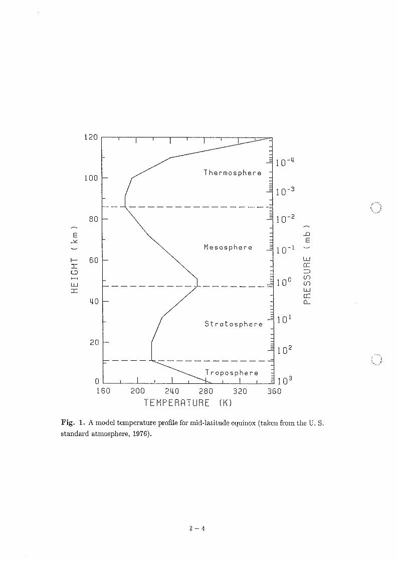
The other common way of dividing regions is the one based o11 the \, ertical structure ofatmospheric temperature. Figure I shows a typical temperature profile, \\, hich is a modelprofile of InId-latitude equinox taken from the U. S. standard atIn OSphere (1976). Theright ordinate shows the atmospheric pressure in millibars. The atmosphere is classifiedinto 4 regions of troposphere, stratosphere, meSOSphere, and the rinosphere in ascendingorder of height

The troposphere is cliaracterized by a constant decrease ill tell}perature witli neight.The lapse rate of the model is 6.5 K km~'. The nT. atn neat source for' this region is thesolar radiation absorbed by the surface of the ear'th. Tel}Tperature ceases to decreaseat 10-15 kin, at the tropopause. The height of the tropopause liar a clear Iatitudinalvariation, being highest in the equatorial region and decreasing witli increasing latitude

The stratosphere is the region in which temperature increases with height. The stablestratification of the air due to positive temperature gradient accounts for the origin of thename of this region. Temperature reaches its maximuin of about 270 K around 50 kinat the stratopause height. The heat source for this maximum is the absorption of solar

2-3

120

100

,-~

E-><

80

^,

I-

^CD

LLl

:Z

50

I^. I

Thermos phere

LID

20

I O ~'

Me SOS phere

2L!O 280

TEMPERi:;TURE (1<)

Fig. I . A model temperature profile for Irud-latitude equinox (taken from the U. Sstandard atmosphere, 1976)

I 0 ~3

I 0 ~2

o

IGO 200

10~'

Strotosphere

,-~

D

E

100

LLl

IT:.

co

(1)

L.

C.L

Troposphere

101

320

102

1.3360

2-4

4

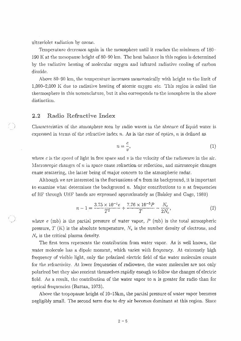
ultra^101et radiation by ozone.

Temperature decreases again in the meSOSphere until it reaclies the minimum of 180-

190 K at the mesopause height of 80-90 kil}. The heat balance in this region is deterIntried

by the radiative heating of molecular oxygen and infrared radiative cooling of carbondioxide.

Above 80-90 kn}, the temperature increases monotonically, \\, it 11 neight to the limit of

1,000-2,000 K due to radiative heating of atomic oxygen etc. This region is called the

thermosphere in this nomenclature, but it also corresponds to the ionosphere in the abovedistinction.

2.2

Characteristics of the atmosphere seen by radio waves in the ajisence of liquid \\, ater is

expressed in terms of the refractive index n. As is the case of optics, n is defined as

Radio Refractive Index

where c is the speed of light in free space and u is the velocity of the radiowa\, e in the air.

Macroscopic changes of n in space cause refraction or reflection, and n\ICroscopic changes

cause scattering, the latter being of major concern to the at In OSpheric radar.

Although we are interested in the fluctuations of n from its background, it is important

to examine what deterTrimes the background n. I\Iaior contributions to n at frequencies

of HE throngli UHF bands are expressed approximately as (Balsley, and Cage, 1980)

3.75 x 10~'e 7.76 x 10~'P N,2N. '

^, here e (Inb) is the partial pressure of water vapor, P (rub) is the total atmospheiic

pressure, T (K) is the absolute temperature, N, is the number density of electrons, andN. is the critical plasma density.

The first term represents the contribution from water vapor. As is well known, the

water molecule has a dipole moment, which varies with frequency. At extremely 111gh

frequency of visible light, only the polarized electric field of the water molecules counts

for the refractivity. At lower frequencies of radiowave, the water molecules are not only

polarized but they also reorient themselves rapidly enough to follow the changes of electric

field. As a result, the contribution of the water vapor to n is greater for radio than for

optical frequencies (Battan, 1973).

Above the tropopause height of 10-15km, the partial pressure of water vapor becomes

negligibly small. The second term due to dry air becomes dominant at this region. Since

C

n=-,U

n-I=T2

+T

(1)

(2)

2-5

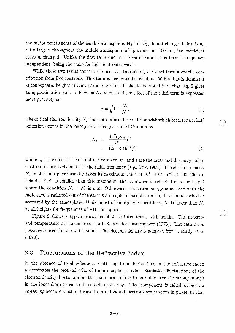
the major constituents of the earth's atmosphere, N2 and 02, do not change their mixingratio largely throughout the middle atmosphere of up to around 100 kin, the coefficientstays unchanged. Unlike the first term due to the water vapor, this term is frequencyindependent, being the same for light and radio waves.

While these two terms concern the neutral atmosphere, the third term gives the con-tribution from free electrons. This term is negligible below about 50 kin, but is dominant

at ionospheric heights of above around 80 kin. It should be noted here that Eq. 2 givesan approximation valid only when N. > N, , and the effect of the third term is expressedmore precisely as

(3)

The critical electron density N, thus determines the condition with whirli total (or perfect)reflection occurs in the ionosphere. It is given in MKS units by

47r e, me 2e2

1.24 x 10~212, (4)

where e. is the dielectric constant in free space, in, and e are the Inass and the charge of anelectron, respectively, and I is the radar frequency (e. 9. , Stix, 1962). The electron densityN, in the ionosphere usually takes its maximum value of 10''-10'' In~' at 200-400 1</11

height. If A', is smaller than this maximum, the radiowa\, e is reflected at solne Ilei 'lit

where the condition N, = N, is met. Otherwise, the entire energy associated witli theradiowave is radiated out of the earth's atmosphere except for a tiny, fractioi} absorbed orscattered by the atmosphere. Under most of ionospheric conditions, N is larger than A1at all heights for frequencies of VHF or higher.

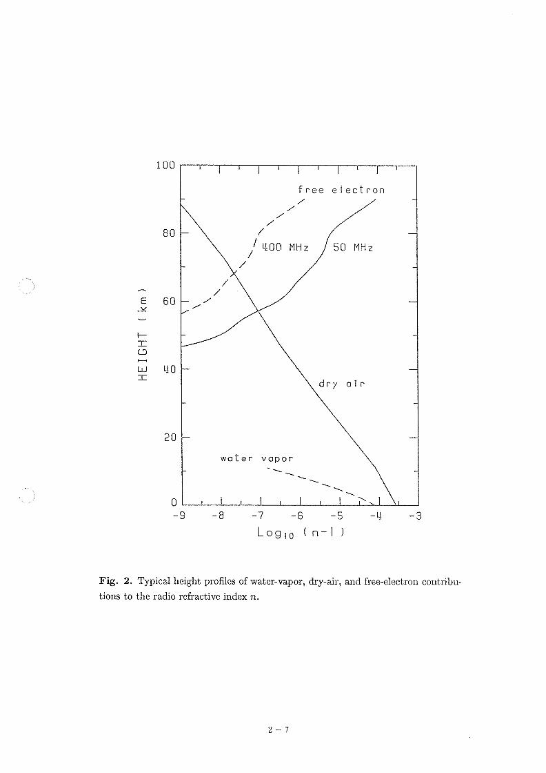
Figure 2 shows a typical variation of these three terms witlL height. The pressureand temperature are taken from the U. S. standard atmosphere (1976). The saturationpressure is used for the water vapor. The electron density is adopted fron} Allechtly at o1.(1972).

N,n= I-=

N'

N

2.3

In the absence of total reflection, scattering from fluctuations in the refractive indexn dominates the received echo of the atmospheric radar. Statistical fluctuations of the

electron density due to random thermal motion of electrons and ions call be strong enou, ,I^in the ionosphere to cause detectable scattering. This component is called incohe?. entscatterin9 because scattered wave from individual electrons are random in phase, so that

Fluctuations of the Refractive Index

2-6

100

80

^

E_>C

~-,

60

I-

ITECD

LLl

:E

free electronI

1100 MHzI

IIII

I

,^I

I

I

II

L!O

50 MHz

20

o

woter

Fig. 2. Typical height profiles of water-vapor, dryair, and free-electron contribu-tions to the radio refractive index n

-9

dry

vopor

-8

GIF

^^

-7 -S -5

Logjo I n-I ,

^...\

~\^

\.

\

- 11 -3

2-7

they add up incoherently. Received echo power is then proportional to the number ofelectrons illuminated by the radar.

Fluctuations due to atmospheric turbulence is known to be the major source of scat-termg in the lower and the middle atmosphere. This component is often called cohe?. Grit

scatterin9 in contrast to the incoherent scattering in the ionosphere. The main difference

of the coherent scattering from the incoherent scattering is that the fluctuation of n iscaused by macroscopic motion of air parcels, each of whicli contains a large number ofmolecules and/or electrons whicli contribute to the scattered electric field coherently illphase. As a result, the scattered echo power is roughly proportional to the square of tilenumber density of scatterers instead of the linear proportionality of the incoherent scatter-

ing. This substantial enhancement in the echo power is the basis for the MsT (Me SOSphereStratosphere Troposphere) radars being able to observe the neutral atnTospliere witli arelatively small system compared to powerful incoherent-scatter radars.

A large difference of the atmosphere from other targets of radars is its distributednature. while usual targets as airplanes, ships, cars, or missiles, \vhicli are referred

to as hard taroets based on their physical nature, have clear boundary \vhicli enablesidentification of the target, it is usually absent in spatial distribution of the echo fromthe atmosphere. It is thus necessary to distinguish parts of the atmosphere by 1110ans ofspatial coordinates of direction and range. This type of target is often called as the softtaroet.

A direct consequence of this limitation, for example, is the fact that decreasing thesize of identified volume in order to improve spatial resolution results in a decrease ill the

echo power, and thus a decrease in sensitivity. On the other hand, the rate of decrease

of the echo power with increasing range to the target is inncli slower witli the soft targetthan with the hard target, because the volume, and thus the size of the scatterer, usuallyincreases with increasing range in case of the soft target.

Mathematical relations which determine the strength of the echo are derived in thefollowing section.

2-8

J

3 The Radar Equation

In designing a radar system, we first need to know how strong the eclio of interest is. wewill derive a relation between transmitted and received power, called the radar equation,

for \, an ons situations \\, hich concern observations with t. he atmospheric radar.

3.1 The Radar Equation for a Hard Target

Before discussing the scattering from fluctuations in the radio refractive index, let us

first examine a simpler case of the scattering from an isolated liard target located in free

Space. Suppose \\, e transmit radiowave of power P, out of an Qinni-directional antenna

which radiates the power into all directions with uniform strength. The density of the

power Pi passing throngl} a unit area located at a point sufficiently far from the antenna

and perpendicular to the direction of propagation is given by

wliere r is the distance of the point from the transmitting antenna. The antenna used for

a radar usually IRS a strong directivity with whicli a narrow region call be illuminated

selectively. The above equation is thus modified as

P, G,Pi=^,

47rr2

where Gt is the directional 90in, or simply, the gain, of tlie antenna, \\, hicli is a function

of the azimuth and the zenith angles.

we now consider a target located at this point whicli intercepts the po\\, er and scatters

it into various directions. The density of the scattered power P, per unit area at a distance

7' from the target is expressed in ternTs of the scatterin9 cross section o of the target as

P.P, = ^0,

4rr, 2

where o is defined as an effective area of the scatterer, the power illuminating \vliicli area is

scattered isotropically. It should be noted that an alternate parameter of the differential

scotterin9 cross section od EE o14T \\, hith expresses the scattered Do\\, er per unit areaand per unit solid on916 is also used often, and occasionally the difference is not clearlymentioned.

It is known, for example, that a perfectly conducting sphere with a radius much larger

than the \\, ave length of the radar has a scattering cross section equal to its physical cross

sortion (,. 9. , Skol, Ik, 1980).

PtPi=^,

4rr2(5)

(6)

2-9

(7)

If we receive the scattered power with an antenna which has a capability of collectingall power passing through an effectiue area A, , the received power P, is expressed as

(8)P, = P, A, L,

where L is the loss factor which represents various attenuation of the received signal due

to antenna, transmission line, connectors etc. By combining Eqs. 6-8, we obtain

P, G, A, L

This equation gives the received echo power from a given target by a radar, and lience

is called the radar equation. We have so far considered a general case in \vhicli the

transmitting and the receiving antennas are not the sanie. Althougli this type of radar,which is called the histotic radar, or the multi-static radar in case there are more than

one receiving antennas, is used in reality for some applications, it is inucli more common

to use the same antenna both for transmission and reception for simplicity. This type of

radar which uses a single antenna is called the monostotic radar, and we will limit our

discussion below to this type of radars.

The two parameters Gt and A, used in the above equations seenT to indicate, at a

first look, distinct properties of an antenna. There is, however, a useful universal relation

known between the two (Silver, 1951), which is

47rA.G, = ^ (10)

where A = c/I is the radar wavelength. Although A, is a function of direction since Gt isso, it is implicitly assumed that the antenna beam of the radar is pointed to the direction

of the target, so that both Gt and A, take their maximum value.

For a monostatic radar, the radar equation thereby reduces to

"A2LP, = ^9- 0. (11)' ~ 47r)\2r4

This equation gives the basis for radar system design of choosing appropriate transmitter

power Pt and effective antenna area A, for a given target with a scattering cross sectiono at a range r.

The minimum detectable power P, is limited by the noise power P \vhicli contaminates

the received signal from the target. In most cases, the dominant component of the noise is

the white noise which is defined as a random time series of signal witli a uniform frequency

power spectrum within the receiver bandwidth B. The power of white noise produced by

a resistor at a temperature T and for a given bandwidth B is given by (Dicke at o1. , 1946)

(12)P, = kTB

P- O.

(4r"')(4r"")(9)

2 -10

10,000

V'.

\

1,000

"or.,-<or"O_

>"I-

"co

oZ

\\

\

\

100

\

\

\*

\\\

\

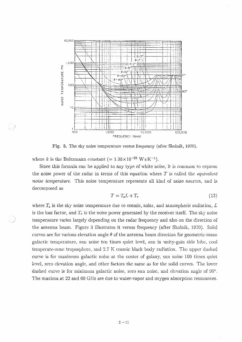
Fig. 3. The sky noise temperature versus frequency (after Skolnik, 1970).

where k is the Boltzmann constant (= 1.38xlO~" WSK~I).Since this formula can be applied to any type of white noise, it is common to express

the noise power of the radar in tern}s of this equation where T is called the eqt, toolent

noise temperature. This noise temperature represents all kind of noise sources, and is

decomposed as

(13)T = T, L + T,

where T, is the sky noise temperature due to cosmic, solar, and atmospheric radiation, L

is the loss factor, and T, is the noise power generated by the receiver itself. The SI<}, noise

temperature varies largely depending on the radar frequency and also on the direction of

the antenna beam. Figure 3 illustrates it versus frequency (after Skolnik, 1970). Solid

curves are for various elevation angle a of the antenna beam direction for geometric-mean

galactic temperature, sun noise ten times quiet level, sun in unity-gain side lobe, cool

temperate-zone troposphere, and 2.7 K cosmic black body radiation. The upper clashed

curve is for maximum galactic noise at the center of galaxy, sun noise 100 times quiet

level, zero elevation angle, and other factors the same as for the solid curves. The 10\\, er

dashed curve is for minimuil} galactic noise, zero sun noise, and elevation angle of 90'.

The maxima at 22 and 60 GHz are due to water vapor and oxygeil absorption resonances

10

I

\!

I 8.1' 1,

;!;

a. 0'

8.90'

~ ~ ~ ~ - - ~U.

8.10

a. 5'

8.30 "

\

2'

\

,

\

\!

.

100

\

\

\

.

,

\

I. 000

FREQUENCY IMHzi

\o'

I

10.000

90'

100,000

2 -11

3.2 The Radar Equation for Distributed Targets

The radar equation derived above applies to a single target. If there are more than one

target in the same volume V of the air observed by a radar, the received electric field is

expressed as the sum of the electric field components caused by individual scatterers. For

a situation where they are random and have no correlation between eacli other, the total

received echo power becomes the sum of the echo power from individual scatter ors. In

this case, the scattering cross section o in Eqs. 7,9, and 11 are simply replaced by :::0. If

the number of scatterers is very large and if scatterers are distributed 11niforn}I^ ill space,

o increases linearly as V increases. It is thereby suitable to define the 001ume reflectiuily

n, or the scattering cross section per unit volume asdo

(14)~ dV'

It should be noted that n has a dimension of jin~'I unlike the ordinary reflectivity, \vhicliis dimensionless.

This situation applies, for example, to the incoherent scattering due to free electrons

in the ionosphere observed \\, ith a sufficiently high frequen^, of above about I GHz, for

which the volume reflectivity is given by

U = N, 0, ,

where o, is the scattering cross section of an electron, \vhicli is given by

47rE;in'c49.98 x 10~" (in').

The condition 'sufficiently higli frequency' is necessary. because otherwise interactions

between electrons and ions througli the Coulomb forces modify significantly the ni. otion

of the electrons reacting to the radar \va\, e field. For a sufficiently low frequency of \/HF

and lower UHF bands, an extra coefficient of 1/2 should be multiplied to the right-hand

side of Eq. 15 (Fejer, 1960-

This type of approacl} based on a microscopic viewpoint is practical only for idealized

situations as discussed above. We need to treat the problem from a more macroscopic

viewpoint of regarding scattering as due to fluctuations in the ref^active index n in order

to discuss the cross section of the neutral atmosphere. Here n is a continuous function of

space, and represents all of the effects caused by scatterers.

The scattered power P, produced by sinall fluctuations of the refractive index All is

expressed formally as ( e. 9. , Doviak and Zrni6, 1984)

Oe

4

(15)

" ' '~';^ 11 An ^,, p(i2k - ")dVl ,

(16)

2 - 12

*

(17)

where k (= 271A) is the radar wavenumber, k is the propagation vector, and r is theradius vector to a point in the scattering \, o1ume. By comparing Eq. 17 \\, it11 Eq. 7, and

applying Eq. 14, we obtain

where () denotes an ensemble average. Although this equation gives a universal expression

for the scattering cross section and the \, online reflectivity, it is not easy, in general, to

perform tile integration to determine C. Specific results will be presented in a separate

chapter

For a uniformly distributed target, V is determined by the spatial resolution of the

radar. Namely, for a radar with a circular antenna, it is expressed in terms of the 11alf-

power beam width of the antenna ah in radians, and the size of the range cell A. r, whichis examined in the next section, as

n

C

k4

T

^^," ^,,,^"', . myI ^

(19)

The beam width of the antenna has a direct relation \\, ith the gain of the antenna Gt

because botli of these paraineters express the degree of concentration of the transnTitted

power of the radar in space. ProbCrt-Jones (1962) expressed the relation as

To 2G* = (-)',

where a is a non-dimensional factor \\, hich concerns the non-uniformity of illumination of

the antenna. Combining this equation with Eq. 10 we obtain

OAa, = - (^ad),

D.

where D, is the effective diameter of the antenna given by 11^:l;. For a circular arrayantenna with uniform excitation for which D, is roughly equal to the physical dialneter

of the antenna, a = I gives a good approximation

With the aid of Eqs. 10,19, and 20, the radar equation Eq. 11 can be rewritten for

distributed targets as

v = r(=)'A"

(18)

64r2

Comparison of this equation with Eq. 11 for a hard target jininediately reveals a

few of interesting features of the scattering from distributed targets. First of all, the

proportionality of the received echo power on the range r is to the square, not to the

P, =PtA. To2ArL

(20)

n

(21)

2 -13

(22)

forth power as is the case for a hard target. This means that the echo power decreases

relatively slowly with increasing r, as mentioned in the preceding section.

Secondly, P, depends only linearly on the effective antenna aperture A. . While the A'factor in Eq. 11 counts for the antenna gain both for transmission and reception, the linear

dependence in Eq. 22 can be interpreted that all of the radiated power is intercepted by the

distributed scatterers, and thus the antenna gain does not count during transmission. It

should also be noted that Eq. 22 does not contain any factor which contains a dependency

on the radar frequency. These properties makes the power aperture product PtA. a good

indication of the sensitivity of an atmospheric radar.

Finally, the ,^. r term in Eq. 22, which does not appear in Eq. 11 means that any

attempt to improve the range resolution of an atmospheric radar should be made at an

expense of reduced sensitivity.

3.3 The Radar Equation for Specular Echoes

We have so far considered two extreme cases of a single target and uniformly distribute(I

target. Although it is not the purpose of this chapter to get into details of \!an ons

scattering mechanisms, let us examine a few more cases for which the radar' equationtakes alternate forms.

The first example is the F1,68nel (or partial) reflection induced by a horizontal layer

which has a slightly different refractive index from that of surrounding air and extends

over a sufficiently wide area. This layer can be treated like a planar mirror, but with

a small reflectivity p for incident electric field (Friend, 1949). Note that p here is thereflectivity in an ordinary sense which has no dimension, and 11as a complex \, alue of

IPI ^ I.The derivation of the radar equation for this case is rather SIInple, because \\, e can

consider the case to be transmission from an antenna to its n}irror 1/1Lagea one-way

located at a distance 2r, with an extra power loss factor of IPI'. Figure 4 shows thesituation schematically. The received power is thus given by

PtGt 2" ' 4, ,(2, )^ A. LIPj

PtA2L 2L, ^,- IPI'";^~IPI (23)

Although the echo power depends on the range by 7' like the case of distributed targets, itis proportional to A'/)\' like that of a hard target. One of important aspects of the Fresnelreflection is its aspect sensitivity. The above equation assumes that the antenna beam is

directed perpendicular to the layer, for which the received echo takes its maximum value.

2 -14

\

mirror ImageI, \

t-. - - - - - ^

IPI' *

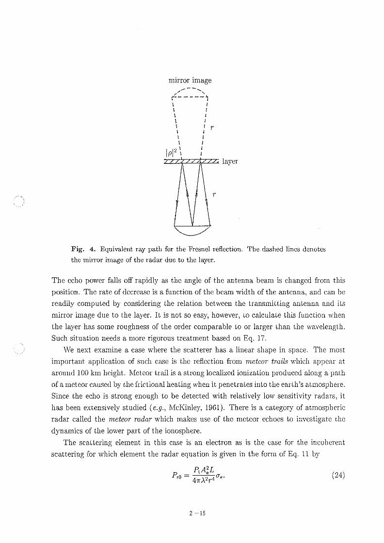
Fig. 4. Equivalent ray path for the F1'esnel reflection. The dashed lines denotes

the mirror image of the radar due to the layer.

The echo power falls off rapidly as the angle of the antenna beam is changed from this

position. The rate of decrease is a function of the beam width of the antenna, and cal} be

readily computed by considering the relation between the transmitting antenna and its

mirror image due to the layer. It is not so easy, however, to calculate this function when

the layer has some roughness of the order coinparable to or larger than the \\, avelengtli.

Such situation needs a more rigorous treatinent based on Eq. 17.

\\Ie next examine a case \\, here the scatterer has a linear shape in space. Tli0 1110st

important application of sricli case is the reflection from meteor trails \\, 111cli appear at

around 100 km height. Meteor trail is a strong localized ionization produced along a path

of a meteor caused by the frictional heating when it penetrates into the earth's atmosphere.

Since the echo is strong enough to be detected with relatively low sensitivity radars, it

has been extensively studied (6.9. , MCKinley, 1960. There is a category of atmospheric

radar called the nieteor radar which makes use of the meteor echoes to investigate the

dynamics of the lower part of the ionosphere.

The scattering element in this case is an electron as is the case for the incoherent

scattering for winch element the radar equation is given in the form of EQ. 11 by

"A2L,0 ~ 4rA2r4 ,.

r

layer

r

2 -15

(24)

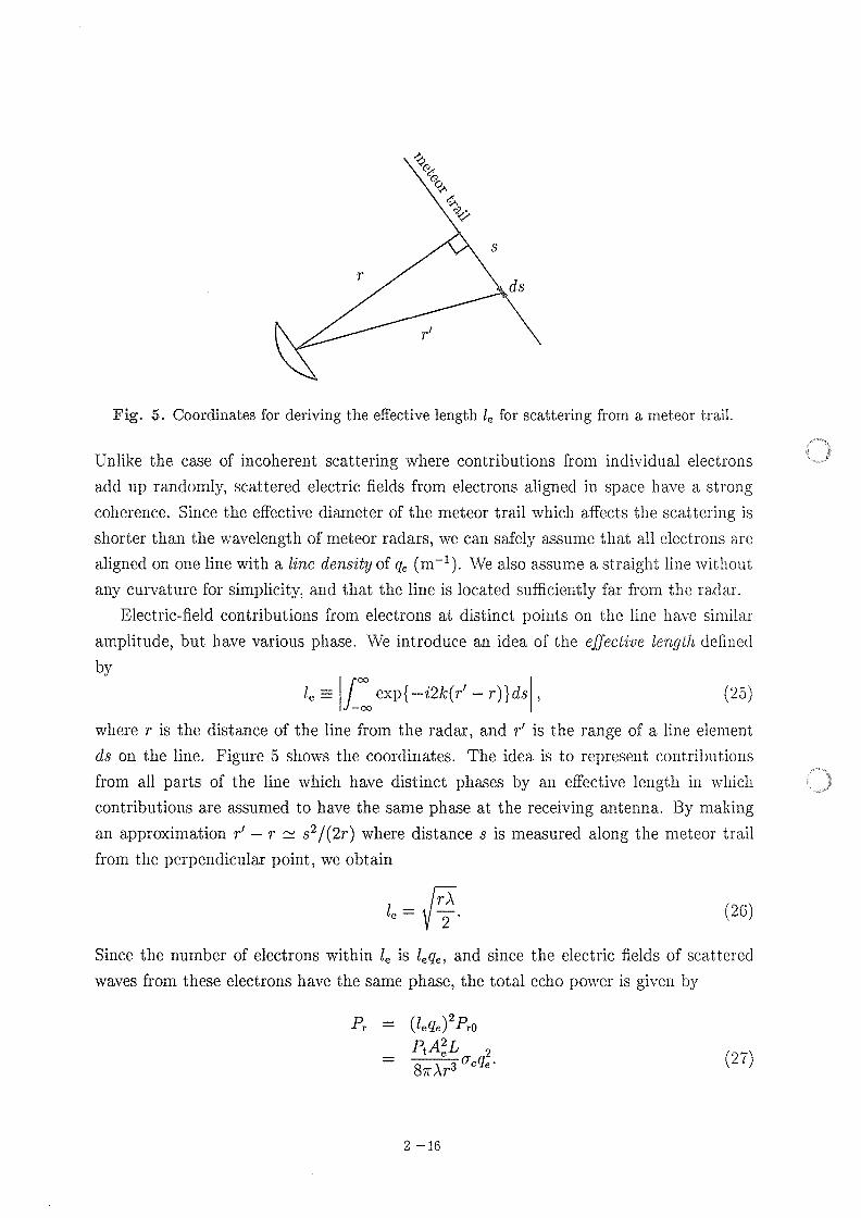
Fig. 5. Coordinates for deriving the effective length I, for scattering from a meteor trail.

Unlike the case of incoherent scattering where contributions from individual electrons

add up randoinly, scattered electric fields from electrons aligned 11} space nave a strontr

coherence. Since the effective diameter of the nTeteor trail \vhicli affects the scattering is

shorter than the wavelength of meteor radars, we can safely assunTe that all electrons an. e

aligned on one line with a line density of q, (in~'). \\'e also assuii}e a straight line \\, itholitany curvature for simplicity, and that the line is located sufficiently far from the radar.

Electric-field contributions from electrons at distinct points on the line 11a\, e similar

amplitude, but have various phase. We introduce an idea of the effectiue Ien9tli defined

by

(25)

where r is the distance of the line from the radar, and r' is the range of a line element

ds on the line. Figure 5 shows the coordinates. The idea is to represent contributions

from all parts of the line which have distinct phases by an effective Iengtli ill \vhicli

contributions are assumed to have the same phase at the receiving antenna. By making

an approximation I - r c>, 8'1(2r) where distance s is measured along the meteor trailfrom the perpendicular point, we obtain

<^,

I

r

I

4>

S

,1

ds

'. I amI-,^^,^", - "^+,, I ,

(26)

Since the number of electrons within I. is I. q, , and since the electric fields of scattered

waves from these electrons have the same phase, the total echo power is given by

P, = (I, q, )'Pro"A2L^-- 0, q, .87rAr3 , ,.

rA^

2 -16

(27)

This equation has a range dependence of r~' which lies between the cases of a hard targetand distributed targets.

3.4

In deriving these radar equations, we have assumed that the target is located at a point

'sufficiently far' from the radar without giving any explicit reason or quantitative limit

for it. Here we examine how large should be the range r in order that equations \\, e havederived are valid, and what happens within this limit.

The antenna of an atmosplieric radar is, whether it is an dish antenna as a paraboloid

or an array of Yagi's or half-wave dipoles, designed to form a beani of the transmitted

\^ave as sharp as possible, because it is the condition to n}animize the gain G, and effectivearea A, as shown in Eqs. 20 and 21. In order to make the beam sharp, it is essential to

produce a planar wavefront over the antenna aperture to the extent as wide as nossible.The transmitted wave thereby propagates as a plane wave at a distance near the antenna

without changing its outer boundary whicli keeps the shape of the antenna aperture. As

it propagates further, it gradually spreads out into a conical region and finally forms aspherical wave with its center located at the center of the antenna aperture.

The region where the \va\, e can be regarded as a planar wave is called the near fieldof the antenna, while the region where it is a spherical wave is called the fin' field. Inanother word, the far field is a region from which the antenna can be seen as a point.This condition is stated mathematicalIy that the distance of a target point measured fi'Qinany point on the antenna aperture falls within a difference sufficiently smaller than thewavelength.

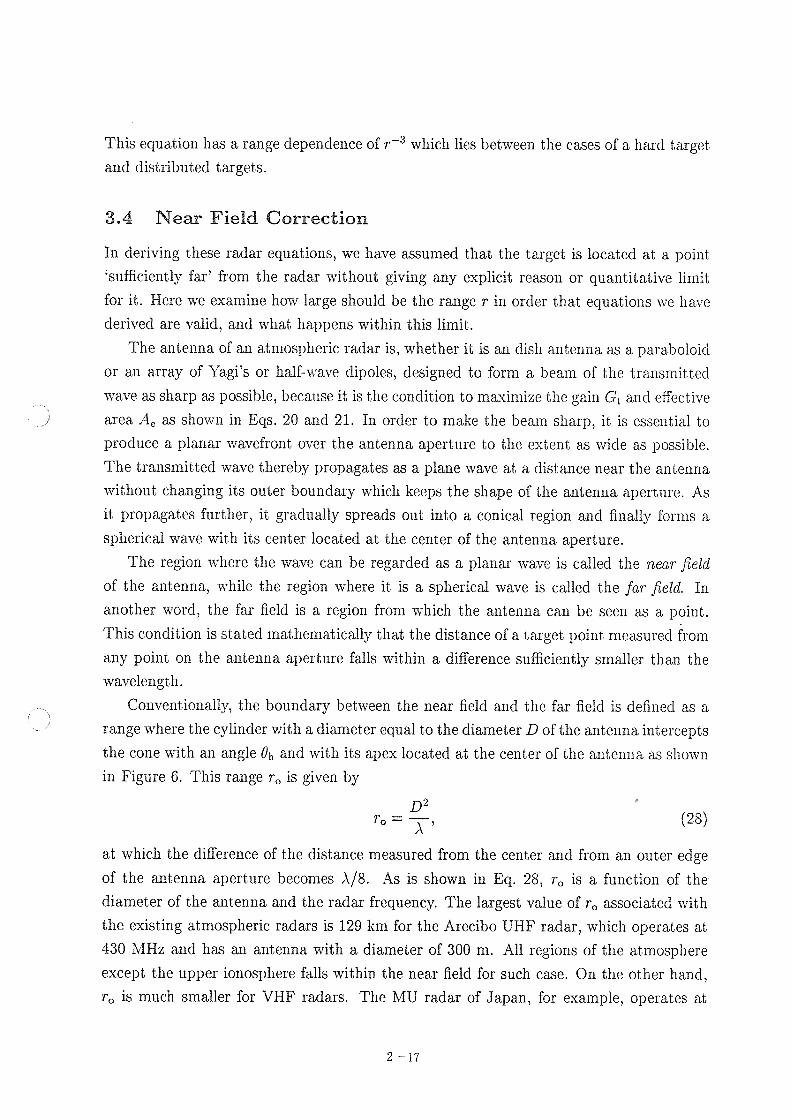
ConventionalIy, the boundary between the near field and the far field is defined as a

range where the cylinder with a diameter equal to the diameter D of the antenna interceptsthe cone with an angle ah and witli its apex located at the center of the antenna as shown

in Figure 6. This range r. is given by

Near Field Correction

h

02(28)A

at which the difference of the distance measured from the center and from an outer ed, re

of the antenna aperture becomes A18. As is shown in Eq. 28, r is a function of the

diameter of the antenna and the radar frequency. The largest value of r associated with

the existing atmospheric radars is 129 kin for the Arecibo UHF radar, which operates at

430 MHz and has an antenna with a diameter of 300 in. All regions of the atmosphere

except the upper ionosphere falls within the near field for such case. On the other hand,

r. is much smaller for VHF radars. The MU radar of Japan, for example, operates at

To '

2 -17

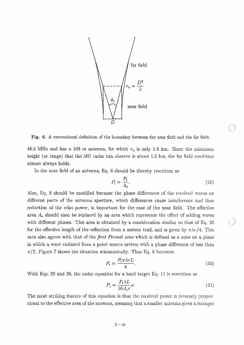
Fig. 6. A conventional definition of the boundary between the near field and the far field.

46.5 MHz and has a 103 in antenna, for which T, is only 1.6 kin. Since the minimunl

height (or range) that the MU radar can observe is about 1.5 kin, the far field condition

almost always holds

In the near field of an antenna, Eq. 6 should be thereby rewritten as

Pt(29)Pi=

A'A,

Also, Eq. 8 should be modified because the phase differences of the received \\, arcs on

different parts of the antenna aperture, which differences cause interference and thus

reduction of the echo power, is important for the case of the near field. The effective

area A. should then be replaced by an area which represents the effect of adding \va\, OS

with different phases. This area is obtained by a consideration similar to that of Eq. 26

for the effective length of the reflection from a meteor trail, and is given by TAT/4. Thisarea also agrees with that of the first F}'esnel zone which is defined as a zone on a plane

in which a wave radiated from a point source arrives with a phase difference of less than

r/2. Figure 7 shows the situation schematically. Thus Eq. 8 becomes

P, TATL

far field

ah

r02

A

D

near field

4

With Eqs. 29 and 30, the radar equation for a hard target EQ. 11 is rewritten as

P, AL(31)P, = -^0.

16A. r

The most striking feature of this equation is that the received power is inversely I)Topor-

tional to the effective area of the antenna, meaning that a smaller antenna gives a stronger

P, =

2 - 18

(30)

echo than a larger one' This is due to the fact that the power density of the transmittedwave is higher for smaller antenna as far as the target is within the near field. It should be

noted, of course, that the upper boundary r. of the near field also decreases as the size of

the antenna is reduced. The other important difference is that the eclio power decreasesonly by r~' with increasing range r in contrast to the very steep r~' decay shown byEQ. 11

Similarly, the radar equation for distributed targets Eq. 22 can be modified for the caseof the near field. Besides the corrections we have made, the scattering volume expressedby Eq. 19 should also be changed as

Fig. 7. Scattering due to a hard target within the antenna near field

C;02CGF,

.-,

=.,

T < To

-first F1'esnel zone

(32)

Applying Eqs. 14 and 32 to Eq. 31, we obtain the radar equation for distributed targetswithin the antenna near field

16r

Note that this equation contains no dependence on the antenna size paran}etcr. \Vliat

EQs. 31 and 33 tells us is that increasing the size of the antenna in order to 111Tj>rove the

sensitivity of the radar works only for targets outside the near field of the antenna

In section 3.3, \\, e also made an implicit assumption that the effective size of the targetfor specular reflections, which is determined by phase coherence of the scattered electric

field, is smaller than the lateral dimension of the beam at that range. It can be shownthat the range at which I. for the meteor trail becomes the same as the beam size is

coincidentally given by r. . The 17 dependence of I. thereby verifies the use of Eq. 27 for

V = A, AT.

P, =P, ATAL

n

2 - 19

(33)

r > T, . A similar condition r > T, /2 can be derived for the validity of Eq. 23 for' Frosnelreflection by considering the condition that the size of the first Fresnel zone of the mirrorimage becomes larger than the size of the antenna.

2 -20

.

.^

4 Basic Techniques

The radar equation derived in the previous section tells us the intensity, of echo, \\, hich

is essential to estimate the necessary transmitter power and the antenna aperture, but

nothing more. In this section, we briefly survey basic techniques used in the atmospheric

radar in determining the range of desired target and also in deriving other inforn}at ion

concerning the target. Details of individual technique will be discussed in following chap-ters

4. L

Ran9in9, or measurement of the range to a target, is one of important functions of radar

we, again, start with the case of observing a hard target. The ranging is made by me a-sunng the time delay of the received echo from the target witli respect to the transmittedsignal

As far as the refractive index n satisfies In - 11 < I, speed of the radio \va\, e can be \\, ellapproximated by that in free space as shown by Eq. I, the error of \vhicli approximation

is given by Eq. 2. In the lower and the middle atmosphere of below about 100 Inn,

In-11 < 10~' as shownin Fig. 2, thence the erroris negligible for allpracticalapplicationsThe error becomes larger, how'ever, ill the ionosphere of above 100 kin depending on thefrequency I and the electron density N, as shown by Eqs. 3 and 4. At a relatively low

frequency of 50 AJIHz, for exainple, the maximum value of n - I during d^, time reaclies~ -0.02 at around the peak neight of F2 region of 200-300 kin. A care n}ust be taken

of tliis error for an accurate ranging of a hard target above the ionospheric neight usinglower VHF band. For oblique beam waves, refraction of the ray patli is not negligibleeither under such condition

Assuming n = I, the range r of a stationary point target is given by

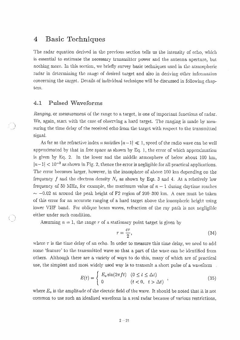
Pulsed Waveforms

(34)

where T is the tinTe delay of an echo. In order to measure this till}e dela^, we need to add

solne feature' to the transmitted wave so that a part of the wa\, e can be identified froin

others' Although there are a variety of ways to do this, many of whicli are of practical

use, the simplest and n}OSt widely used way is to transmit a snort pulse of a \\, aveform

where E, is the amplitude of the electric field of the wave. It should be noted that it is not

common to use such an idealized waveform in a real radar because of various restrictions,

E(t) , I '. Sin(271t) (0 ^; t :^ At'o (t<0, t>,. t)

CT

2 -21

(35)

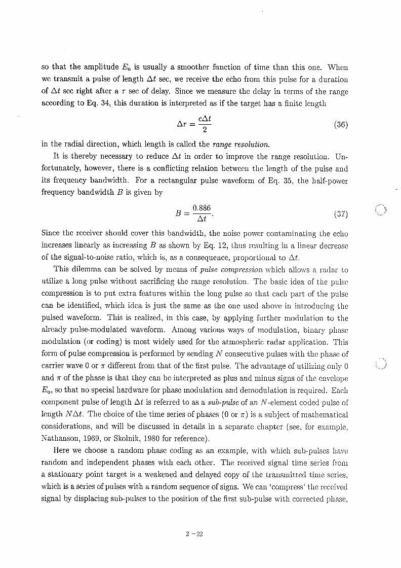
so that the amplitude E. is usually a smoother function of time than this one, When

we transmit a pulse of length At sec, we receive the echo from this pulse for a duration

of At sec right after a r sec of delay. Since we measure the delay in terms of the rangeaccording to Eq. 34, this duration is interpreted as if the target has a finite length

in the radial direction, which length is called the run9e resolution.

It is thereby necessary to reduce At in order to improve the range resolution. Un-fortunately, however, there is a conflicting relation between the length of the pulse andits frequency bandwidth. For a rectangular pulse waveform of Eq. 35, the half-powerfrequency bandwidth B is given by

(37)

Since the receiver should cover this bandwidth, the noise power contaminating the eclioincreases linearly as increasing B as shown by Eq. 12, thus resulting ill a linear decreaseof the signal-to-noise ratio, which is, as a consequence, proportional to At.

This dilemma can be solved by means of pulse compression \vhicli allows a radar to

utilize a long pulse without sacrificing the range resolution. The basic idea of the I}ulsc

compression is to put extra features within the long pulse so that each part of tlie pulse

can be identified, which idea is just the same as the one used above in introducing thepulsed waveform. This is realized, in this case, by applying further modulation to thealready pulse-modulated waveform. Among various ways of modulation, binary phasemodulation (or coding) is most widely used for the atmospheric radar application. Tliisform of pulse compression is performed by sending N consecutive pulses with the phase of

carrier wave O or r different from that of the first pulse. The advantage of utilizing only Oand T of the phase is that they can be interpreted as plus and minus signs of the envelopeE, , so that no special hardware for phase modulation and demodulation is required. Eacli

component pulse of length At is referred to as a sub-pulse of an N-element coded pulse of

length NZ\. t. The choice of the time series of phases (O or r) is a subject of matlieii}atICalconsiderations, and will be discussed in details in a separate cliapter (see, for. exaiilPIG,Nathanson, 1969, or Skolnik, 1980 for reference).

Here we choose a random phase coding as an example, witli whicli sub-pulses 11a\, e

random and independent phases with each other. The received signal time series from

a stationary point target is a weakened and delayed copy of the transmitted time series,

which is a series of pulses with a random sequence of signs. We can 'compress' the received

signal by displacing sub-pulses to the position of the first sub-pulse witli corrected phase,

cAtAr = --

0.886B-

At

(36)

2 -22

r

I\. r

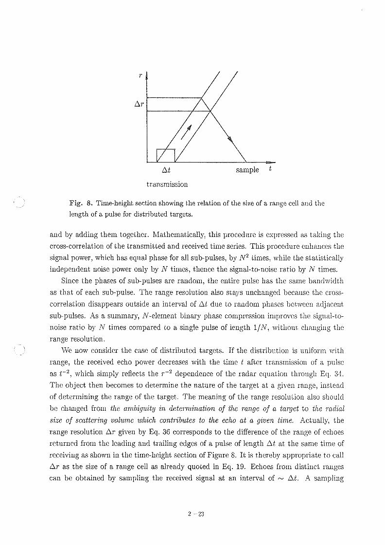
Fig. 8. Time-height section showing the relation of the size of a range cell and the

length of a pulse for distributed targets

and by adding them together. MathematicalIy this procedure is expressed as taking thecross-correlation of the transmitted and received time series. This procedure enhances the

signal power, which has equal phase for all sub-pulses, by N' times, while the statisticalIyindependent noise power only by N times, thence the signal-to-noise ratio by N tin}es

Since the phases of sub-pulses are random, the entire pulse has the same bandwidth

as that of each sub-pulse. The range resolution also stays unchanged because the cross-

correlation disappears outside an interval of At due to random phases between adjacent

sub-pulses. As a summary, A'-element binary phase compression improves the situal-to-

noise ratio by N times compared to a single pulse of Iengtli 11N, without changing tlie

range resolution

we now consider the case of distributed targets. If the distributioi} is uniform with

range, the received echo POW'er decreases with the time t after transmission of a pulse

as t~', which simply reflects the r~' dependence of the radar equation throuoli Eq. 34.The object then becomes to determine the nature of the target at a given range, instead

of determining the range of the target. The meaning of the range resolution also should

be changed from the Qinbi9ttit!I in deterrninotion of the Ton9e of a target to the 70th o1

size of scatterin9 volume which contributes to the echo at a 9iuen time. Actually, the

range resolution ,^. r given by Eq. 36 corresponds to the difference of the range of eclioes

returned from the leading and trailing edges of a pulse of Iengtli At at the sinne tiine of

receiving as shown in the time-height section of Figure 8. It is thereby appropriate to call

A. r as the size of a range cell as already quoted in Eq. 19. Echoes from distinct ranges

can be obtained by sampling the received signal at an interval of ~ z\. t. A sampling

I

transniission

,:^. t sample

2 -23

interval of less than At produces overlapping regions between the samples, \\, hile a spars

sampling results in missing regions. It is therefore common to salnple at all interval justequal to I\. t. The sampled time series provides a range (or usually, neight) profile of theatmosphere. \\Ie should note that the impulsive sampling intended by Fig. 8 does notrepresent a realistic situation where the receiver has a bandwidtli equal to that of the

transmitted pulse. In this case, an instantaneous sample of receiver output contains the

echo spreads over a duration of A, t. Although this effect broadens the range cell froii} arectangular shape of width AT into a triangular one of width 2Ar, the 'half-power' size

of the cell is still given by z\, r.

As we have seen, the signal-to-noise ratio is proportional to the hangtli of pulse Atfor the case of a hard target. For the case of distributed targets, we need to take intothe account the linear proportionality of echo power on AT as shown ill Eq. 22, \\, it ich

represents the nuniber of scatterers in a range cell. The signal-to-noise ratio thus be conies

proportional to At', setting a severe restriction in improving the range resolution. Forexample, dividing a single pulse into A1 sub-pulses with binary phase coding illTprovcs the

range resolution by N times without sacrificing the signal-to-noise ratio of a hard taroot,while the same alteration offers the same improvement only at an expense of a reduction

of the signal-to-noise ratio to 11N for the case of distributed targets.

4.2 The Doppler Principle

we have so far concentrated our attention only to the echo power. Physical 1110aiiingof the echo power is, however, clear only for the case of incoherent scattering froiiT t, heionosphere, for which case it can be interpreted in terms of the electron density. It isdifficult to make use of the echo power from the lower and the middle atmosphere 11} a

quantitative manner in terms of physical parameters of geophysical interests.

The Doppler shift of the echoes, on the other hand, has a great importance for' these

regions as well as for the ionosphere, because it is directly related to the niotioii of the

target, which is wind. The Doppler frequency shift of echoes from a 11Toving target relativeto the radar is given by

Id = ^Ud, (38)

where ud is the line-of-sight component of velocity vector v of the target relative to theradar.

Since the maximum velocity encountered in the atmosphere is on the order of 100 nis~'

If, I < I kH^ for any freqneney I of ness than I GH^. A typical wine of I, f0" 50 MH^ bandis, for example, around 3 Hz, which corresponds to a line-of-sight veloci^, of 10 In s~' .

C

2 -24

t

.

Bandwidth of transmitted pulses is, on the other hand, 100 kHz-I MHz corresponding tothe minimum length of sub-pulses of I-10 IIS. It is thereby very difficult, if not impossible,to detect such small Doppler shift of a pulse relative to its bandwidtli from earn received

pulse.

Instead, the method of time-series analysis is applied to the series of received signalfrom consecutive pulses at the same range. If a stationary target is observed, all receivedpulses should have the same phase relative to the transmitted pulse. It is then interpretedthat the received time series has the DC component only, which means that the Doppler

shift is zero. Next we suppose that the target is moving at a sufficiently slow speed ofud in the radial direction so that it does not move out of a range cell into the next one

within the period of interest. we examine samples of echoes obtained at the same rangecell from adjacent pulses separated by an inter-pulse-period (IPP) of T. Tlieii the phasedifference A4i between the two samples is given by

4rfTA. 4) = 2ndT = ^ud. (39)

This equation can be applied not only to a hard target but also to distributed tartrcts asfar as they move with a mean speed of lid. The phase difference call be determined fron}

a pair of pulses, while the Doppler frequency shift Id can be directly derived by a spectralanalysis of the time series of samples taken from many, pulses.

A limitation of this method arises from the requirement 1,411 < r so that Id can bedetermined without ambiguity, together with the one T > 27 IC \vhicli comes from therestriction that we cannot transmit a new pulse before receivino the echo of the previous

pulse from the longest range rinax of interest. By combining these two requirements, weobtain

(40)

which gives the condition that both the range and the velocity of a target can be de-termined uriambiguously. Since the quantities on the left-hand side of this equation are

limited roughly by 100 in s~' x 100 kin = 10' in's~' this condition is usually satisfied fora frequency of below about I GHz, which is the frequency used for atmospheric radars.

Considerations made above assumes that the echo is perfectly correlated in time, which

assumption is not valid for the case of the atmospheric radar, where echoes nave finite

correlation time T. due principalIy to random motion of scatterers within a scatteringvolume. This correlation time is inversely proportional to the spectral broadening due tothe random motion and other observational effects, and given by

b bcT -^

c of 210, '

C

2

I", hmm, , < -,max 81 '

2 -25

(41)

where of and o, denote the standard deviation of the random motion in terms of Dopplerfrequency and radial velocity, respectively, and b is a numerical coefficient of order unitywhich is determined by the velocity distribution of the random motion. For a Gaussiandistribution, b = 1.18.

The value of o, differs largely depending on the height, since it is the order of meanthermal motion of ions of more than I kms~' in the ionosphere, while it is the meanvelocity of turbulent eddies of the order of I in s~' in the lower and the middle atmosphere.For ionospheric observation, for which o, > ud, the ud term in Eq. 40 should be replacedby o, , which determines spectral width and thus the minimum sampling interval. It iseasily understood that the condition for uriainbigiious sampling is then no more satisfied,meaning that spectral information of the scatterers must be derived within an interval of

order of r. . A special technique called multi-pulse method was developed for ionosphericobservations, and has been widely used (e. 9. , Farley, 1969).

4.3 Velocity Field Measurements

As shown in Eq. 38, velocity of targets measured by a radar with the Doppler techniqueis a line-of-sight velocity, which is the projection of velocity vector to the radial direction.

We will briefly examine here two distinct techniques of determining the three componentsof the velocity vector: the Doppler-Beam-Sum9 (DBS) method and the Spaced-Antenna-D"tit^ (SAD) meth. d.

The DBS method makes use of multiple antenna beams each of \vhicli is oriented to

observes the radial velocity at a different direction. The velocity vector is coinputed froiTithe line-of-sight velocities from these directions. Here we need to make an assumptionthat the velocity field is uniform in space over the volume which contains the range cellsused to compute a velocity vector. In the atmospheric radar application, it is coilTinon

to determine a velocity vector from line-of-sight velocities of range cells witli the sameheight assuming the uniformity only in the horizontal plane, so that a 1101glit I>To fileof the velocity vector can be obtained. This is because the horizontal velocity is IISuallymuch larger than the vertical velocity in the stratified earth's atmosphere, thus Inaking thehorizontal uniformity of the velocity field much better than in the vertical direction. Also,the fact that the zenith angle of antenna beams is usually kept within about 30's up portsthis assumption, in contrast to the case of weather radars, which use almost norizontalbeam directions,

The line-of-sight component of the wind velocity vector v = (u ,u ,I) ) at a given

2 -26

.-

height is expressed as

u, cos a, + U, Cos 0, + 11, cos a, , (42)

where i is a unit vector along the antenna beam direction, and a, , a , and 8 are the anglebetween i and the ", 31, and z axis, respectively. If we measure lid at three beam directions

ii, i2, and i3 which do not constitute a plane, we can obtain an estimate of v as

lid

If we observe more than three directions, then the estimate of v can be determined in

a least-squares manner, with which the residual given by the following is nTinimized :

e, , ^ >:(u, cos a, j + U, cos a, j + 11, cos eat - u, ,)2, (44)

where in is the number of beam directions. The necessary condition for v to give theminimum is that partia. I derivatives of 5' with respect to all three components of v are

062

^ ' 0 (j ' ", 11, ^). (45)

This set of equations can be solved in terms of v as

V. I.

I'"'"2, Cos8,2, cos8,21~ 1/'d2j'V=

zero:

Vn

i=I

V=

>:: cos' 0, ,, >: cos O, jcos 8, j, Z cos a, t cos 8, j Z udi cos 8, I

>: cos art cos eat, ^: cos a, , cos a, ,, >:: cos' 0, , Z lid, cos art

\^here the summations are taken for i = I to in.

A special case of this type of multi-beam measurements called the Velocity-AzimuthDisplay (VAD) method, which uses beam directions with a fixed zenitli angle 8 anduniformly distributed azimuth angles 41j. The lineof-sight velocity ud of Eq. 42 is thenrewritten as

Udj ' Uh Sin a Sin(4^j + ,) + I), Cos a, (47)

where Iih and , are the amplitude and the direction of the horizontal component of r,respectively, and given by

(43)

I)h

,

02 , ,, 2

mm-" (,) .

2 -27

Z

VVd

Vy

V

O 90 180 270 360

'A ( deg )

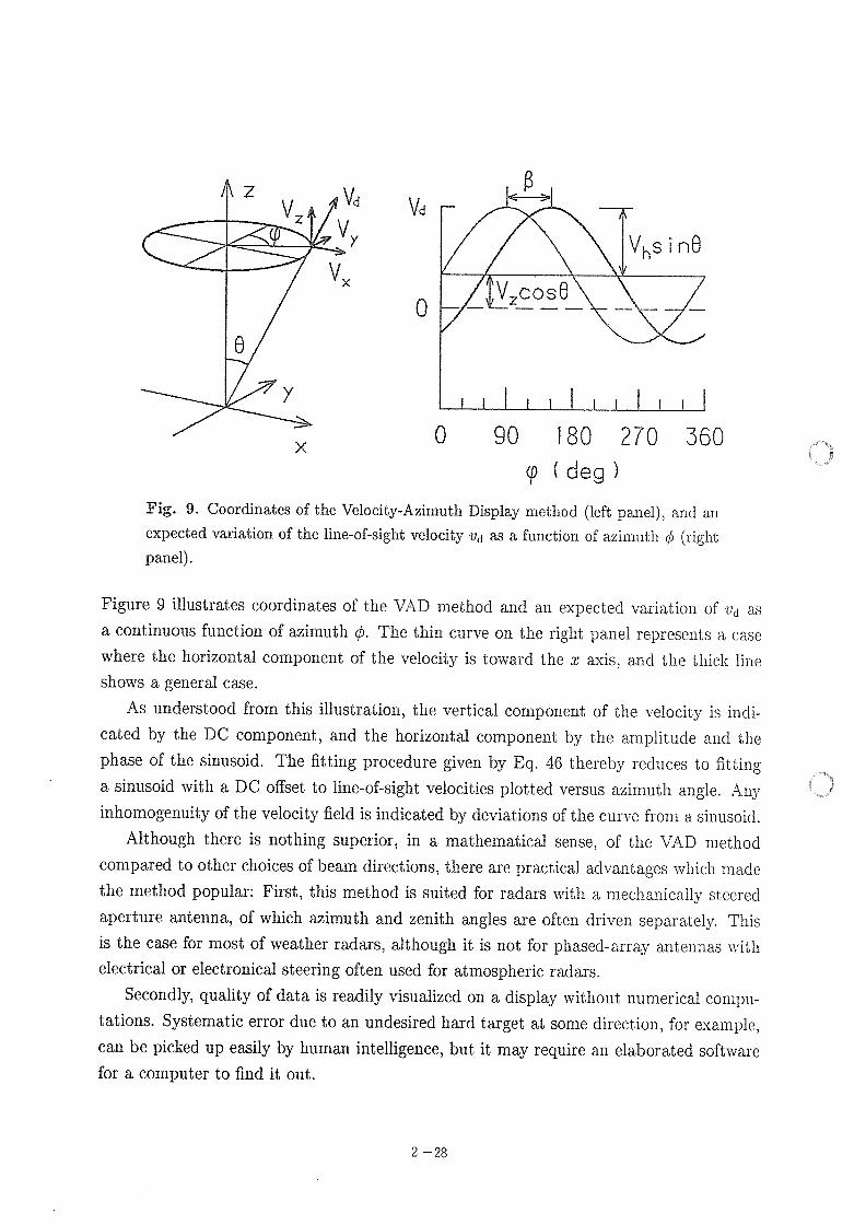
Fig. 9. Coordinates of the Velocity-Azimuth Display method (left panel), aild anexpected variation of the lingof-sight velocity ud as a function of azimut11 4^ (rightpanel).

Figure 9 illustrates coordinates of the VAD method and an expected vanatioiL of u asa continuous function of azimuth (b. The thin curve on the right panel represents a GISowhere the horizontal component of the velocity is toward the r axis, and the thic1< 11/10shows a general case.

As understood from this illustration, the vertical component of the velocit is indi-cated by the DC component, and the horizontal component by the ainplitude and thephase of the sinusoid. The fitting procedure given by Eq. 46 thereby reduces to fittina sinusoid with a DC offset to line-of-sight velocities plotted versus azimuth an Ie. Aninhornogenuity of the velocity field is indicated by deviations of the curve front a sinusoid.

Although there is nothing superior, in a mathematical sense, of the VAD method

compared to other choices of beam directions, there are practical advantages \vhicli Inadethe method popular: First, this method is suited for radars \\, ith a Ineclianically steeredaperture antenna, of which azimuth and zenith angles are often driven separately. Thisis the case for most of weather radars, although it is not for phased-array antennas withelectrical or electronical steering often used for atmospheric radars.

Secondly, quality of data is readily visualized on a display without I}umerical coinpu-tations. Systematic error due to an undesired hard target at some direction, for example,can be picked up easily by human intelligence, but it may require an elaborated softwarefor a computer to find it out.

e

Vd

I

o

X

V, cos^

Vhs i nO

2 -28

.

Thirdly, a systematic error due to specular echoes from the vertical direction call be

avoided with the VAD method by choosing the zenith angle 8 properly. The specular

echoes from horizontally stratified layers often dominate over isotropic scattering fronT

turbulence (Cage and Green, 1978, R6ttger and Liu, 1978), which make the apparent

zenith angle of the antenna beam direction smaller than the physical one for beam di-rections near the vertical direction. This effect is most prominent for lower stratospheric

region, where data from beam directions with small zenith angles n}ust be treated \\, ith

care (Tanda at at. , 1986)This caution applies, of course, to all DBS observations. On the other nand, use of

too large zenith angle makes the assumption of a uniform velocity field unreliable

The alternate technique of the Spaced-Antenna-Drifts n}ethod Inakes efficient use of

this specular echoes in determining norizontal velocities. It was originally developed to

study characteristics of irregularities in the lower ionosphere (6.9. , Ratcliffe, 1956), and

applied to observations of velocities in the middle atmosphere (e. ,., \/incent at o1. , 1977)

and lower atmosphere (8.9. , Rottger and Vincent, 1978). Its principle is to 11}easure a

spatial correlation of received signal patterns from a reflecting layer witli spaced antennas

on the ground.

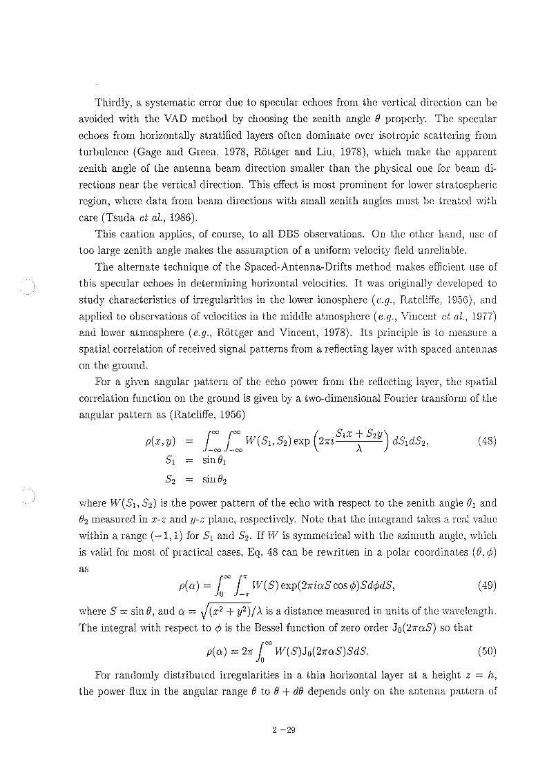
For a given angular pattern of the echo power from the reflecting layer, the spatial

correlation function on the ground is given by a two-dimensional Fourier transform of the

angular pattern as (Ratc}life, 1956)

co co SIT + 8211- 00 - 00

Sin 81

Sin 02

where W(SI, S2) is the power pattern of the echo with respect to the zenitli angle 01 and

82 measured in r-z and 11-z plane, respectively. Note that the integrand takes a rea. I \, aluc

within a range (-I, I) for SI and S2. If W is symmetrical with the azin}utli angle, \\, hich

is valid for' most of practical cases, Eq. 48 can be rewritten in a polar coordinates (a, 4;)

P(", u)

SI

S2

as

P(0) = 100 I TV(S) exp(2"ms cos ^#)Sd4^dS,where S = sin 8, and a = 111^!'11)\ is a distance measured in units of the \\, a\, Glength

p(a) = 2^ 100 W(S)J, (2^OS)SdSThe integral with respect to 41 is the Bessel function of zero order J0(2roS) so that

(50)

For randomly distributed irregularities in a thin horizontal layer at a height z = h,

the power flux in the angular range a to O + d8 depends only on the antenna nattern of

(48)

2 -29

(49)

I- o

\^. ~.\~^ ~.~

08

\\\

p(a)

06

\

\\

\

\

\

\

\

\

DJ

\

\

\

\

\

\

\\\

\

02

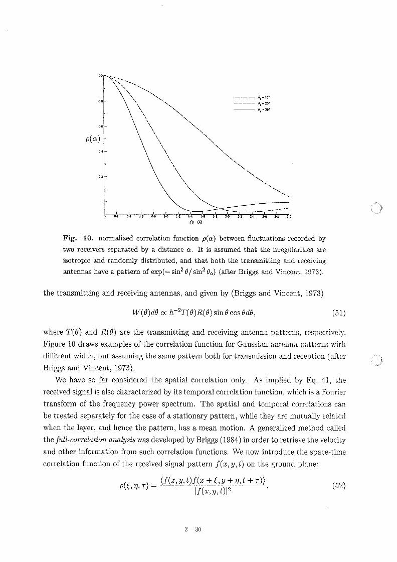
Fig. 10. normalized correlation function p(a) between fluctuations recorded by

two receivers separated by a distance or. It is assumed that the irregularities are

isotropic and randomly distributed, and that both the transmitting and receiving

antennas have a pattern of exp(- sin' 81 sin' a. ) (after Briggs and Vincent, 1973).

the transmitting and receiving antennas, and given by (Briggs and Vincent, 1973)

W(a)d8 or h~'T(0)R(a) sin a cos 8d8, (51)

where T(0) and R(a) are the transmitting and receiving antenna patterns, respectively.Figure 10 draws examples of the correlation function for Gaussian antenna I)at terns with

different width, but assuming the same pattern both for transmission and reception (after

Briggs and Vincent, 1973).

We have so far considered the spatial correlation only. As implied by Eq. 41, the

received signal is also characterized by its temporal correlation function, \vhicli is a Fourier

transform of the frequency power spectrum. The spatial and temporal correlations can

be treated separately for the case of a stationary pattern, while they are mutually related

when the layer, and hence the pattern, has a mean motion. A generalized 11}ethod called

the full-correlation analysis was developed by Briggs (1984) in order to retrieve the velocity

and other information from such correlation functions. We now introduce the space-tnne

correlation function of the received signal pattern I(r, 11, t) on the ground plane:

(A", v, t)I(" + ^, v + n, t + ^))

\

\

\

\

\

\

\\

\

D

\

\

\\

\

o

\

\

\

02

-.-.-. 6. .I0f- --- ,.. 20', a. . 30'

.\

\\

\

04

\

\

\

\

\

us

\

\

\

08

\

\

\\

\

Iu

\

\

\

1.2 14

\

\

\

\

\\

\

alay

\ .~ ~

I6

\\

1.8 2 0 z 2 2.4

~~---

\

\\\\

----------

\\

2.6 2-, 3.0

\

P(^, n, ^) =If (", v, t)I'

2 -30

,

(52)

where () means to take an ensemble average, which is often replaced by a temporal averagein practical applications. This correlation function represents the statistical relations of

the signal pattern at two points with a separation (^, n) on the ground and witli a timedifference of r. We assume that for a stationary pattern, the correlation function 11as aform

P(^, n, ^) = p(A^' + Bn' + K^' + 2H<n). (53)

This assumption implies that the spatial and temporal correlations have the same func-

tional shape, but the shape is arbitrary. Although this is not real in a rigorous sense,it is an acceptable approximation for most of correlation functions at least around their

origin.

We next suppose that the pattern is moving at a velocity V = (V, , V ). If we Inove thecoordinates also at this velocity, then Eq. 53 remain unchanged for the 11Loving coordinates.the expression for the stationary coordinates is therefore obtained after a linear transforiiTof coordinates that

P(^, n, T) = p{A(^ - V, T)' + B(n - V, T)' + Kr' + 2H(^ - V, T)(11- \'!T)I,

which is rewritten as

P(^, n, r) = p(A<' + Bn' + KT' + 2F^r + 2GnT + 2H^n). (55)

If we have two spaced receivers, \\, e ca. n determine the shape of the cross-correlation

as a function of T for a given set of (^, n). Since Eq. 55 is a function of a second-order

polynomial of T, it is possible to determine three unknowns by fitting it to the measuredcross-correlation function. It is thus clear that three spaced receivers, \vhicli provides IIS

two sets of independent cross-correlation functions, is sufficient to determine all coefficients

in Eq. 55. If we have more than three receivers, we can determine the coefficients ill aleast-squares manner as is the case of the DBS method.

Once the coefficients are determined, we can retrieve the velocity, vector V froiii these

coefficients. By comparing Eqs. 54 and 55, we obtain

AV, + HV

By, + HV,

These equation can be readily solved to give (V, , V ). The vertical component of the

velocity vector needs to be determined separately from the Doppler shift of the echo.

An important point which needs to be mentioned is that an apparent velocity V'

calculated from the distance between the receivers and the time delay which gives the

maximum value of the cross-correlation function does not agree witli the true \, o10city

(54)

-F

-G

2 -31

(56)

T

No wind W i F1 d V

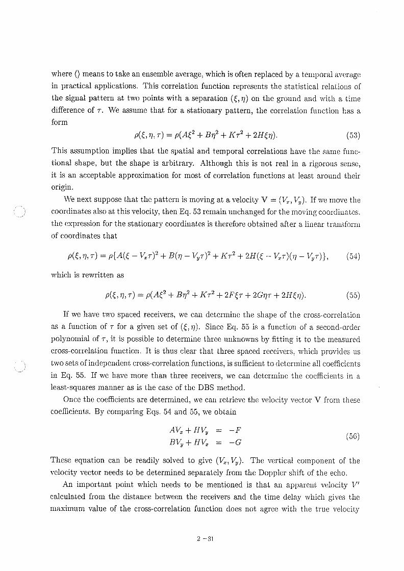
Fig. 11. Contours of equal correlation versus distance ^ and time delay T. Theleft panel shows a case with no mean wind, and the right panel is witl} a uniformwind. The true velocity V estimated with the fun-correlation anal sis is denoted

by the solid line. The dashed line indicates the apparent velocit V' determinedfrom the time delay of maximun} correlation.

V of the pattern, which is correctly estimated with the full-correlation anal SIS. These

two time delays coincide when the temporal correlation of the pattern is perfect, \\, hichmeans that the pattern is drifting without evolving with time, while a finite correlationtime significantly affects the shape of the cross-correlation function.

Figure 11 illustrates this difference schematically. The left panel shows concentric cir-cles which represent contour lines of equal correlation versus distance ^ along the baselineand the time delay T for a case of no mean motion. The abscissa and the ordiiiate arc

normalized by the correlation distance and the correlation time of the pattern, so that thecontours become circles instead of ellipses. If a mean motion of V is added, the contoursdeform into ellipses as shown in the right panel. Note that the solid line \\, hicli indicatesthe true velocity V is drawn by connecting tangential points of the ellipses with norizontallines as implied by Eq. 54.

Since the cross-correlation function with respect to r at a distance ^ is given by thevalues of contours along a line of constant ^ (i. e. , a vertical line), V' obtained fromits maximum has a slope indicated by the dashed line in the figure, \vhicli is drawn b ,connecting tangential points of ellipses with vertical lines. The difference between the true

velocity V and the apparent velocity V' therefore becomes larger as V becomes sriialler.One of reasons that the full-correlation analysis is widely used is that it is free Iron} this

T

I

V

I

II

V

2 -32

-

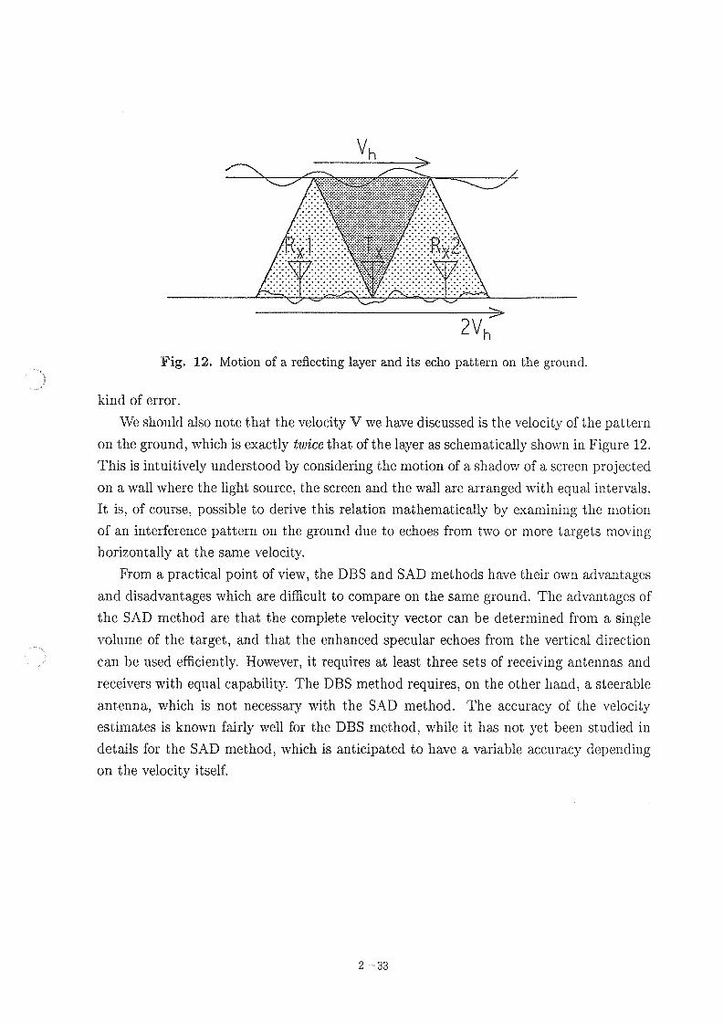
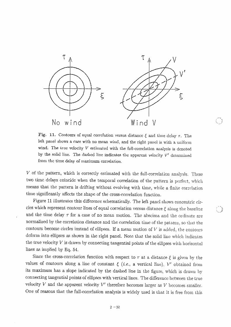
2VhFig. L2. Motion of a reflecting layer and its echo pattern on the ground.

kind of error.

\\/e should also note that the velocity V we have discussed is the velocity of the pattern

on the ground, which is exactly twice that of the layer as schematically shown in Figure 12.

This is intuitively understood by considering the motion of a shadow of a screen projected

on a wall where the light source, the screen and the wall are arranged witli equal intervals.

It is, of course, possible to derive this relation mathematicalIy by examining the n}otion

of an interference pattern on the ground due to echoes from two or more targets nTovinghorizontally at the same velocity.

From a practical point of view, the DBS and SAD methods have their own advantages

and disadvantages which are difficult to compare on the same ground. The advantages of

the SAD method are that the complete velocity vector can be determined from a single

volume of the target, and that the enhanced specular echoes from the vertical direction

can be used efficiently. However, it requires at least three sets of receiving antennas and

receivers with equal capability. The DBS method requires, on the other hand, a steer able

antenna, which is not necessary with the SAD method. The accuracy of the \, elocity

estimates is known fairly well for the DBS method, while it has not yet been studied ill

details for the SAD method, which is anticipated to have a variable accuracy dependingon the velocity itself.

Vh

. . ................................. . .

2 -33

References

Balsley, B. B. , and K. S. Gage, The MsT radar technique: Potential for middle atino-

spheric studies, Pure Appl. Geophys. , 11.8,452-493,1980.

Battan, L. J. , Radar Observation of the Atmosphere, The University of Chicago Press,

Chicago, 1973.

Briggs, B. H. , The analysis of spaced sensor records by correlation technique, Handbook

for MAP, 1.3,166-186, 1984.

Briggs, B. H. , and R. A. Vincent, Some theoretical considerations on remote probing of

weakly scattering irregularities, AUSt. I. Ph!/s. , 26,805-814,1973.

Dicke, R. H. , R. Beringer, R. L. Kyhl, and A. B. Vane, Atmospheric absorption In Gasure-

merits with a microwave radiometer, Ph!/s. Reu. , 70,340-348, 1946

Doviak, R. J. , and D. S. Zrni6, Doppler Radar Grid Weather 068eruotions, ACadeinic

Press, London, 1984.

Earley, D. T. , Multi-pulse incoherent-scatter correlation function measurei}Tents, Radio

Sci. , 4,935-953, 1969

Fejer, J. A. , Scattering of radio waves by an ionized gas in thermal equilibriuin ill the

presence of a uniform magnetic field, Con. I. Ph!!, s. , 39,716-740, 1961

Friend, A. W. , Theory and practice of tropospheric sounding by radar, Proc. Inst. Radio

Bit9. , 37,116-138,1949

Gage, K. S. , and J. L. Green, Evidence for specular reflection from monostatic VHF radar

observations of the stratosphere, Radio Sat. , 13,991-1001,1978

MCKinley, D. W. R. , Meteor Science and En9ineerin9, McGraw-Hill, New York, 1961

Mechtly, E. A. , S. A. Bowhill, K. P. Gibbs, and L. G. Smith, Changes of lower ionosphere

electron concentrations with solar activity, I. Atmos. Terr. Ph!Is. , 34, 1899-1907,1972.

Nathanson, F. E. , Radar Desi9n Principles, McGraw-Hill, New York, 1969

Ratcliffe, J. A. , Some aspects of diffraction theory and their applicatioi} to the ionosphei. e,

Rep. Pro9r. Ph!/s. , 19,188-267,1956

Rottger, J. , and C. H. Liu, Partial reflection and scattering of VHF radar signals from

the clear atmosphere, Geoph!/s. Res. Lett. , 5,357-360, 1978.

R6ttger, J. , and R. A. Vincent, VHF radar studies of tropospheric velocities and irregu-

Ianties using spaced antenna techniques, Geoph!Is. Res. Lett. , 5,917-920,1978

2 -34

Silver, S. , Micrott!one Antenna Theory and Desi9n, McGraw-Hill, New York, 1951.

Sk. link, M. L. (^ditor), Radar Handbook, M, Grow-Hill, Non York, 1970.

Skolnik, M. L. , Introduction to Radar Systems, McGraw-Hill, New York, 1980

Stix, T. H. , The Theory of Plasma ryoues, McGraw-Hill, New York, 1962

Tsuda, T. , T. Sato, K. Hirose, S. F1ikao, and S. Kato, MD radar observations of the aspect

sensitivity of backscattered VHF echo power in the troposphere and lower stratosphere,Radio Sci. , 21,971-980,1986

Vincent, R. A. , T. J. Stubbs, R. H. 0. Pearson, K. H. Lloyd, and C. H. Low, A comparison

of partial reflection drifts with winds determined by rocket techniques - I, I. AtntosTen, . Ph!Is. , 39,813-821,1977.

2 -35