PROGRAMA BIOEN Projeto 2008/56156 0 Use and Agriculture ... · Projeto 2008/56156 ... Simulating...
23
Instituto de Estudos do Comércio e Negociações Internacionais Local: São Paulo, 09/02/2011 Simulating Land Use and Agriculture Expansion in Brazil: Food, Energy, Agro‐industrial and Environmental Impacts PROGRAMA BIOEN Projeto 2008/56156‐0 “Simulating Land Use and Agriculture Expansion in Brazil: Food, Energy, Agro‐industrial and Environmental Impacts” Relatório Científico Final (9 de Fevereiro de 2011) Pesquisador Responsável: André Meloni Nassar Instituição Sede: Instituto de Estudos do Comércio e Negociações Internacionais (ICONE) Equipe de Pesquisa: Leila Harfuch, Pesquisadora ICONE Marcelo M. R. Moreira, Pesquisador ICONE Luciane C. Bachion, Pesquisadora ICONE Laura B. Antoniazzi, Pesquisadora ICONE Rodrigo C. Lima, Pesquisador ICONE Período de Vigência: 01/08/2009 a 31/12/2010
Transcript of PROGRAMA BIOEN Projeto 2008/56156 0 Use and Agriculture ... · Projeto 2008/56156 ... Simulating...

Instituto de Estudos do Comércio e Negociações Internacionais
Local: São Paulo, 09/02/2011
Simulating Land Use and Agriculture Expansion in Brazil: Food, Energy, Agro‐industrial and Environmental Impacts
PROGRAMA BIOEN Projeto 2008/56156‐0
“Simulating Land Use and Agriculture Expansion in Brazil: Food, Energy, Agro‐industrial and Environmental Impacts”
Relatório Científico Final (9 de Fevereiro de 2011)
Pesquisador Responsável: André Meloni Nassar Instituição Sede: Instituto de Estudos do Comércio e Negociações Internacionais (ICONE) Equipe de Pesquisa: Leila Harfuch, Pesquisadora ICONE Marcelo M. R. Moreira, Pesquisador ICONE Luciane C. Bachion, Pesquisadora ICONE Laura B. Antoniazzi, Pesquisadora ICONE Rodrigo C. Lima, Pesquisador ICONE Período de Vigência: 01/08/2009 a 31/12/2010
Instituto de Estudos do Comércio e Negociações Internacionais
Simulating Land Use and Agriculture Expansion in Brazil: Food, Energy, Agro‐industrial and Environmental Impacts 1
Item I: Summary of the Objectives “Simulating Land Use and Agriculture Expansion in Brazil: Food, Energy, Agro‐industrial and
Environmental Impacts”
In the era of searching for energy security and reducing green house gas (GHG) emissions, agricultural‐based biofuels have been considered the alternative energy source. In addition with the growing demand for agricultural commodities, the international debate has been focused on the land use change impacts coming from the increasing demand for biofuels.
As an “emerging agricultural sector”, Brazilian agriculture is expanding and increasing its importance in the world market. Brazil has tremendous potential to be, not only an important supplier of traditional agricultural commodities, but also an important global biofuel supplier, especially of sugarcane ethanol. As exposed in the project proposal, many questions arise regarding land use change effects, specially related to the competition among crops and pasture and also the effects on the agricultural frontier.
The methodologies currently available to assess land use changes due to biofuel and agricultural expansion are incomplete and need to be improved. Economic models and other methodologies fail to capture and replicate empirical evidence about the agricultural sector, land allocation and land use changes dynamics.
The best approach to deal with the uncertainties of measuring GHG savings from agricultural‐based biofuels, in addition to biofuel expansion and its effects on food production and prices (food versus fuel debate), is to calibrate economic parameters based on historical land use changes identified by satellite imagery and remote sensing techniques, along with secondary data.
The main objective of this project is to calibrate parameters in the Brazilian Land Use Model (BLUM) in order to capture and replicate empirical evidence and the dynamics of the agricultural sector from a prospective point of view.
Since the satellite imagery database was available during the development of this project, BLUM parameters were re‐calculated. Combining better available information with cause‐effect method results, it was possible to turn the competition among crops and pasture and the definition of the determinants of total area allocated to agriculture into parameters in the model.
In order to achieve the main objective of this project and to answer the questions raised in the project proposal, the following specific objectives were considered in this study:
(i) Establishment of the individual contribution of agricultural uses in total agricultural land expansion; (ii) Re‐calibration of land supply elasticities for the six regions included in BLUM land use module; (iii) Definition of a new ranking for the competition among agricultural uses with the objective of
increasing the competition between crops and pastures; (iv) Re‐calibration of own and cross competition elasticities for agricultural uses included in BLUM that
compete for land (soybean, rice, cotton, corn first crop, sugarcane, dry beans first crop and pastures);
(v) Sensitive analysis comparing the previous version of the model and the updated one.
For the first specific objective, the individual contribution in total land allocated to agriculture is measured as the share of each product in total land brought into production. This parameter is used in the calculations to establish the re‐calibrated land supply elasticities and own and cross competition elasticities, which were revised using satellite images database combined with secondary database analysis.
Land supply elasticities are the parameters that govern the expansion of total agricultural area as a function of changes in profitability. Since empirical evidences are available to determine the responsibility of each agricultural activity over deforestation, the agricultural area response to average return (land supply elasticities) shall be recalculated.
Instituto de Estudos do Comércio e Negociações Internacionais
Simulating Land Use and Agriculture Expansion in Brazil: Food, Energy, Agro‐industrial and Environmental Impacts 2
For the third item, the competition ranking was used in the calculations of cross competition elasticities. Since there is evidence that crops are displacing pasturelands, the competition among crops and pasture might be higher than among different crops. As so, this evidence needs to be captured by the cross competition elasticities.
The study shows the connections among all the elasticities and the need to recalculate all of them using satellite images database combined with cause‐effect methodology. Own and cross competition elasticities govern area response of individual products to changes in returns. As in land supply elasticities, own and cross elasticities were re‐calibrated by BLUM regions and are presented as competition matrices.
Finally, the last specific objective is to simulate a scenario with ethanol demand shock in order to compare the results of the previous and updated versions of the BLUM. Based on the U.S. Renewable Fuel Standard, the demand shock was, approximately, 9 billion liters of additional ethanol exports (comparing to the baseline scenario).
Through parameters that capture the agricultural sector dynamics, it is possible to make multiple inferences using the model´s results. Capturing the competition among grains, sugarcane and pasture can answer the questions raised in the food versus fuel debate, such as: how biofuel expansion affects food prices and total production; what happens in the agricultural frontier when one activity is displaced by a biofuel feedstock; if there are any change on the regional production dynamics; how different policies affect agricultural dynamics; among many others.

Instituto de Estudos do Comércio e Negociações Internacionais
Simulating Land Use and Agriculture Expansion in Brazil: Food, Energy, Agro‐industrial and Environmental Impacts 1
Item II: Main Achievements “Simulating Land Use and Agriculture Expansion in Brazil: Food, Energy, Agro‐industrial and
Environmental Impacts”
1. Introduction
Since the end of 2007 the Institute for International Trade Negotiations (ICONE) has been working on improving the methodologies used for measuring the impacts of the expansion of the agricultural sector on land use in Brazil. The main purpose of this research agenda is to quantify direct and indirect land use changes (LUC and iLUC) of agricultural‐based biofuels in general and sugarcane ethanol in particular. In a partnership with the Center for Agricultural and Rural Development (CARD, Iowa State University), ICONE´s research team developed an economic model called Brazilian Land Use Model (BLUM) to simulate supply and demand of agricultural products produced in Brazil and its impacts on the demand for land,. Because BLUM is integrated to FAPRI´s world models (FAPRI, 2010)1 it is possible to simulate the responses of the Brazilian agricultural sector to changes in world prices.
Besides economic modeling, ICONE is also working with other methodologies to quantify land use changes as a consequence of the expansion of agricultural‐based biofuels (Nassar et al., 2011a)2. The institute developed a deterministic methodology to estimate GHG land use emissions associated to the expansion of sugarcane (Nassar et al., 2010 3; Nassar et al., 2011b 4).
Economic models require constant updates of data, parameters and assumptions. A key issue regarding ICONE´s research agenda on land use was to improve BLUM´s land allocation and competition section ‐ land use module – incorporating new data, recalibrating parameters and revising assumptions that determine equations used in the model. Through the combination of data generated in the context of the deterministic methodology, remote sensing data assessing Cerrados biome conversion to annual crops and pastures (Ferreira et al., 2011)5, data on Amazon, Cerrados and Atlantic Forest biomes deforestation and data on the agricultural sector´s per hectare profitability listed in BLUM, ICONE was able to update and improve BLUM´s land allocation and competition section.
The improvements accomplished in BLUM´s land use section are discussed and presented in this report as the main achievements of the project “Simulating Land Use and Agriculture Expansion in Brazil: Food, Energy, Agro‐industrial and Environmental Impacts”. This report also presents the results of a set of BLUM simulations comparing the previous structure of the land use module to the new one.
The establishment of parameters and assumptions that govern land allocation for BLUM´s agricultural sectors based on real data is a key methodological contribution of this project. Land supply elasticities (response of total agricultural land to changes in market returns) and cross‐area elasticities (response of the area of a certain agricultural use to changes in the return of another use) were recalculated using historical data of land use changes from satellite images, rather than based on secondary data only. The
1 FAPRI. 2010 U.S. and World Agricultural Outlook. Food and Agricultural Policy Research Institute. FAPRI Staff Report 10‐FSR 1. 2 Nassar, A. M.; Harfuch, L.; Bachion, L. C.; Moreira, M. R. 2011a Biofuels and land‐use changes: searching for the top model. Interface Focus (doi:10.1098/rsfs.2010.0043). This reference is listed in item V as a publication resulting from this project. 3 Nassar, A. M.; Antoniazzi, L. B.; Moreira, M. R.; Chiodi, L.; Harfuch, L. 2010 An Allocation Methodology to Assess GHG Emissions Associated with Land Use Change: Final Report. ICONE (report and detailed spreadsheet available at http://www.iconebrasil.com.br/en/?actA=8&areaID=8&secaoID=73&artigoID=2107). 4 Nassar, A. M.; Moreira, M. R.; Antoniazzi, L. B.; Bachion, L. C.; Harfuch, L. 2011a Indirect land‐use changes for sugarcane ethanol in Brazil: Development of a causal allocation methodology. Energy Policy (submitted but not accepted yet). This reference is listed in item VI as a publication resulting from this project. 5 Ferreira, M. E.; Silva, J. R.; Rocha, G. F.; Antoniazzi, L.; Nassar, A.; Rocha, J. C. S. Caracterização das áreas desmatadas no bioma Cerrado via sensoriamento remoto: uma análise sobre a expansão de culturas agrícolas e pastagens cultivadas. XV Simpósio Brasileiro de Sensoriamento Remoto (submitted and accepted). This reference is listed in item V as a publication resulting from this project.
Instituto de Estudos do Comércio e Negociações Internacionais
Simulating Land Use and Agriculture Expansion in Brazil: Food, Energy, Agro‐industrial and Environmental Impacts 2
assumptions that drive the contribution of individual agricultural sectors to the conversion of the agricultural frontier, as well as those that govern the competition among agricultural uses, were also revised based on evidences from remote sensing data and satellite imagery.
The main achievements of this project are:
(i) Establishment of the individual contribution of agricultural uses in total agricultural land expansion. The individual contribution is measured as the share of each product in total land brought into production (Table 3);
(ii) Re‐calibration of land supply elasticities for the six regions included in BLUM land use module. Land supply elasticities are the parameters that govern the expansion of total agricultural area as a function of changes in profitability (Table 5);
(iii) Definitions of a new ranking for the competition among agricultural uses with the objective of increasing the competition between crops and pastures. The competition ranking was used in the calculations of cross competition elasticities;
(iv) Re‐calibration of own and cross competition elasticities for agricultural uses (soybean, rice, cotton, corn first crop, sugarcane, dry beans first crop and pastures) that compete for land included in BLUM. Own and cross competition elasticities govern area response of individual products to changes in market return. As in land supply elasticities, own and cross elasticities were re‐calibrated according to BLUM region and are presented in competition matrices (Table 6, Table 7, Table 8 to Table 13);
This report is organized as follows. BLUM land allocation is described in the next section. Section 3 discusses the methodological developments of the project in terms of data generation and the theoretical model used. Section 4 is devoted to present the results of estimated parameters and simulations. The final section offers a set of recommendations and points out limitations associated to this project´s results.
2. BLUM Land Allocation Section6
BLUM comprises the following products: soybeans, corn (first and second crop), cotton, rice, dry beans (first and second crop), sugarcane, wheat, barley, dairy, and livestock (beef, broiler, eggs and pork). Commercial forests are considered exogenous projections. Combined, these activities were responsible for 95 percent of total area used for agricultural production in 2008.7 Although second and winter crops, such as corn, dry beans and wheat do not generate additional need for land (they are smaller and planted in the same place as first season crops), their production is accounted for in the national supply.
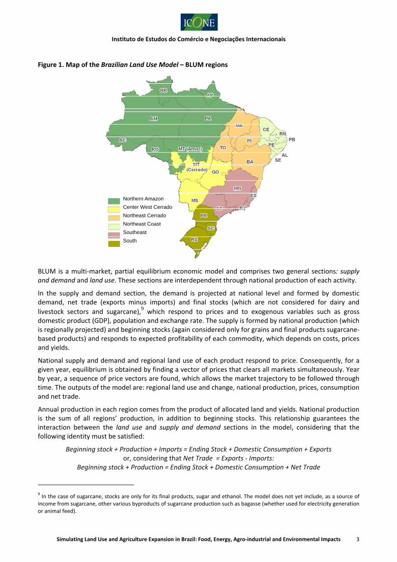
Land allocation for agriculture and livestock is calculated for six regions,8 as showed in Figure 1:
South (states of Paraná, Santa Catarina, and Rio Grande do Sul);
Southeast (states of São Paulo, Rio de Janeiro, Espírito Santo, and Minas Gerais);
Center‐West Cerrado (states of Mato Grosso do Sul, Goiás and part of the state of Mato Grosso inside the biomes Cerrado and Pantanal);
Northern Amazon (part of the state of Mato Grosso inside the Amazon biome, Amazonas, Pará, Acre, Amapá, Rondônia, and Roraima);
Northeast Coast (Alagoas, Ceará, Paraíba, Pernambuco, Rio Grande do Norte, and Sergipe);
Northeast Cerrado (Maranhão, Piauí, Tocantins, and Bahia).
6 This section is focused on the land use section of the model. The structure of the supply and demand section is described in detail in the section 7.3. of the submission of this project to Auxílio à Pesquisa/Projeto Temático. 7 When we refer to agricultural area, we consider annual crops, sugarcane and livestock. 8 The main criteria to divide the regions were agricultural production homogeneity and individualization of biomes with especial relevance for conservation.
Instituto de Estudos do Comércio e Negociações Internacionais
Simulating Land Use and Agriculture Expansion in Brazil: Food, Energy, Agro‐industrial and Environmental Impacts 3
Figure 1. Map of the Brazilian Land Use Model – BLUM regions
BLUM is a multi‐market, partial equilibrium economic model and comprises two general sections: supply and demand and land use. These sections are interdependent through national production of each activity.
In the supply and demand section, the demand is projected at national level and formed by domestic demand, net trade (exports minus imports) and final stocks (which are not considered for dairy and
livestock sectors and sugarcane),9 which respond to prices and to exogenous variables such as gross
domestic product (GDP), population and exchange rate. The supply is formed by national production (which is regionally projected) and beginning stocks (again considered only for grains and final products sugarcane‐based products) and responds to expected profitability of each commodity, which depends on costs, prices and yields.
National supply and demand and regional land use of each product respond to price. Consequently, for a given year, equilibrium is obtained by finding a vector of prices that clears all markets simultaneously. Year by year, a sequence of price vectors are found, which allows the market trajectory to be followed through time. The outputs of the model are: regional land use and change, national production, prices, consumption and net trade.
Annual production in each region comes from the product of allocated land and yields. National production is the sum of all regions’ production, in addition to beginning stocks. This relationship guarantees the interaction between the land use and supply and demand sections in the model, considering that the following identity must be satisfied:
Beginning stock + Production + Imports = Ending Stock + Domestic Consumption + Exports or, considering that Net Trade = Exports ‐ Imports:
Beginning stock + Production = Ending Stock + Domestic Consumption + Net Trade
9 In the case of sugarcane, stocks are only for its final products, sugar and ethanol. The model does not yet include, as a source of income from sugarcane, other various byproducts of sugarcane production such as bagasse (whether used for electricity generation or animal feed).
Northern Amazon
Center West Cerrado
Northeast Cerrado
Northeast Coast
Southeast
South
Instituto de Estudos do Comércio e Negociações Internacionais
Simulating Land Use and Agriculture Expansion in Brazil: Food, Energy, Agro‐industrial and Environmental Impacts 4
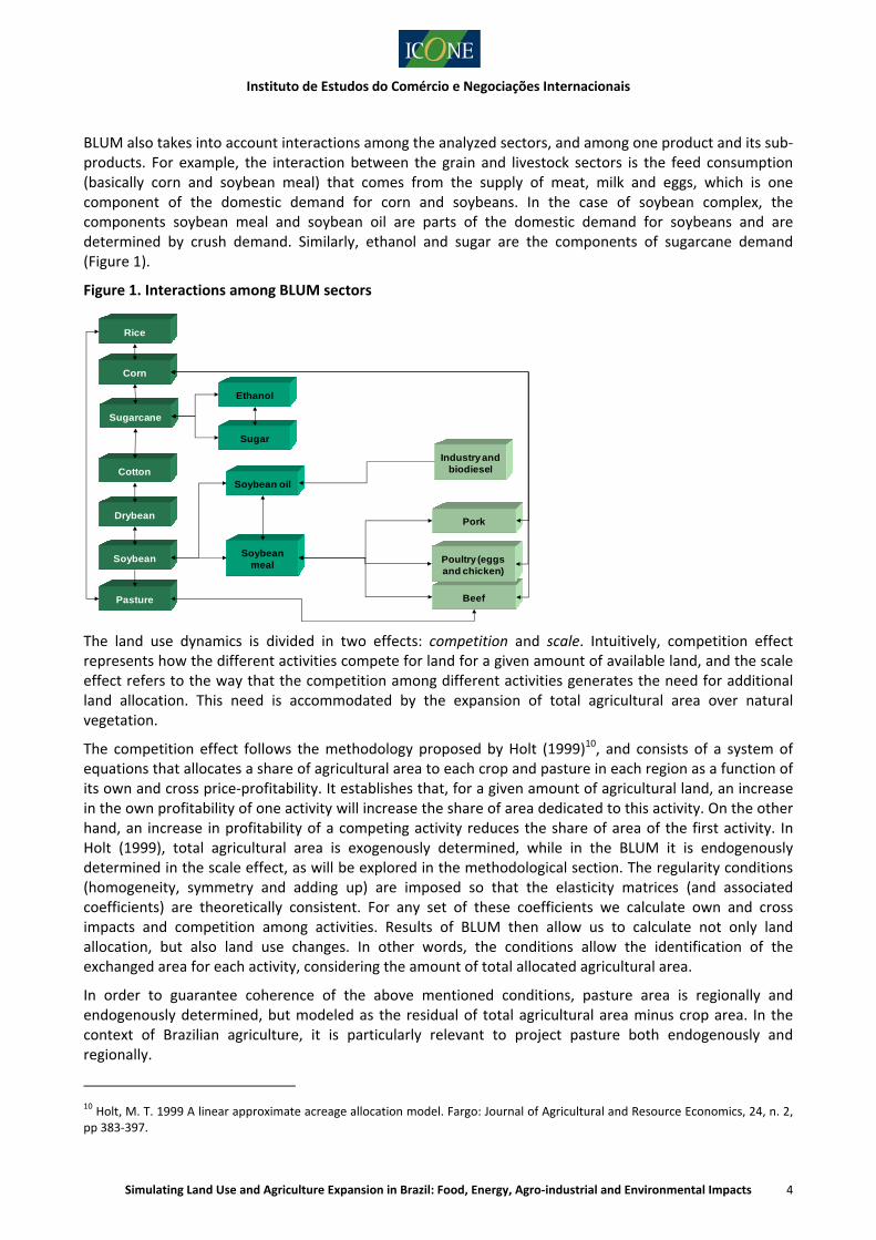
BLUM also takes into account interactions among the analyzed sectors, and among one product and its sub‐products. For example, the interaction between the grain and livestock sectors is the feed consumption (basically corn and soybean meal) that comes from the supply of meat, milk and eggs, which is one component of the domestic demand for corn and soybeans. In the case of soybean complex, the components soybean meal and soybean oil are parts of the domestic demand for soybeans and are determined by crush demand. Similarly, ethanol and sugar are the components of sugarcane demand (Figure 1).
Figure 1. Interactions among BLUM sectors
The land use dynamics is divided in two effects: competition and scale. Intuitively, competition effect represents how the different activities compete for land for a given amount of available land, and the scale effect refers to the way that the competition among different activities generates the need for additional land allocation. This need is accommodated by the expansion of total agricultural area over natural vegetation.
The competition effect follows the methodology proposed by Holt (1999)10, and consists of a system of equations that allocates a share of agricultural area to each crop and pasture in each region as a function of its own and cross price‐profitability. It establishes that, for a given amount of agricultural land, an increase in the own profitability of one activity will increase the share of area dedicated to this activity. On the other hand, an increase in profitability of a competing activity reduces the share of area of the first activity. In Holt (1999), total agricultural area is exogenously determined, while in the BLUM it is endogenously determined in the scale effect, as will be explored in the methodological section. The regularity conditions (homogeneity, symmetry and adding up) are imposed so that the elasticity matrices (and associated coefficients) are theoretically consistent. For any set of these coefficients we calculate own and cross impacts and competition among activities. Results of BLUM then allow us to calculate not only land allocation, but also land use changes. In other words, the conditions allow the identification of the exchanged area for each activity, considering the amount of total allocated agricultural area.
In order to guarantee coherence of the above mentioned conditions, pasture area is regionally and endogenously determined, but modeled as the residual of total agricultural area minus crop area. In the context of Brazilian agriculture, it is particularly relevant to project pasture both endogenously and regionally.
10 Holt, M. T. 1999 A linear approximate acreage allocation model. Fargo: Journal of Agricultural and Resource Economics, 24, n. 2, pp 383‐397.
Cotton
Rice
Drybean
Corn
SoybeanSoybean
meal
Soybean oil
Sugarcane
Ethanol
Sugar
Beef
Pork
Poultry (eggs and chicken)
Pasture
Industry and biodiesel
Instituto de Estudos do Comércio e Negociações Internacionais
Simulating Land Use and Agriculture Expansion in Brazil: Food, Energy, Agro‐industrial and Environmental Impacts 5
Although the competition among activities may represent regions where the agricultural area is sTable and near its available potential, this is an insufficient analysis for Brazil. Recent Brazilian agricultural history shows that crops, commercial forests and pastures combined respond to market incentives by contributing to an expansion of the total area allocated to agriculture. This effect is captured in the scale section of the BLUM. This methodological improvement is essential to adjust the model skills to the specific reality of Brazilian agricultural land use dynamics.
The scale effect refers to equations that define how the returns of agricultural activities determine the total land allocated to agricultural production. More precisely, total land allocated to agriculture is a share of total area available for agriculture, and this share responds to changes in the average return of agriculture. For each region, total land allocated to agricultural production is projected as:
,*Re AturnAvgfAgland
where Agland is total land allocated to agricultural production, turnAvg Re is the average agricultural
return of the region, A is the total available land (that was estimated using geospatial information), .f is
a constant elasticity function with results in the interval [0,1] for reasonable values of average return.
However, scale and competition effects are not independent. In conjunction, they are the two components of the own return elasticities of each activity. Considering a ceteris paribus condition, the increase in profitability of one activity has three effects: increase in total agricultural area (through average return), increase in its own share of agricultural area and, therefore, reduction in the share of agricultural area of other activities. For competing crops, cross effects of profitability on area are negative.
As mentioned previously, the own elasticities of each crop are the sum of competition and scale elasticities. At the same time, regional elasticity of land use with respect to total agricultural returns (total Agland elasticity) is the sum of the scale elasticities of each activity. Therefore, competition elasticities can be calculated directly after total Agland elasticity while total own elasticities were obtained through econometric analysis and literature review. The option to estimate area response to return, instead of price, is supported by several studies.11 The process to obtain proper elasticities was comprehensively discussed by ICONE and CARD/FAPRI staffs until the final values were agreed on.
Own return elasticity was mainly estimated through time series econometric analysis, using official data for area, namely from Brazil’s Agriculture Ministry’s National Supply Agency (CONAB) and the Brazilian Institute of Geography and Statistics (IBGE). Annual profitability was calculated by ICONE. Literature review and experts were also consulted for qualitative ranking of elasticities. Table reports the own area‐return elasticities (averaged by area) used in BLUM for crops and pasture in this paper.
Specific geospatial analysis was conducted in order to estimate total potential land available for agricultural production for each BLUM region, which is included as an input in the scale effect section of the model. Two databases are available: (i) one developed by UFMG in the context of the Brazil Low Carbon Study and integrated to the SIMBRASIL model (de Gouvello, 201012) and (ii) a second one provided by the Agricultural Land Use and Expansion Model – Brazil (AgLUE‐BR, Sparovek et al., 2010a13). For restricting agricultural land use expansion physical (soil, climate and slope) and legal (environmental legislation applicable to private farmland and public conservation parks) conditions were also spatially considered.
11 Bridges, D.; Tenkorang, F. 2009 Agricultural Commodities Acreage Value Elasticity Over Time: Implications for the 2008 Farm Bill. San Diego: American Society of Business and Behavioral Sciences. v.6, n.1. 12 de Gouvello, C. 2010 Brazil Low Carbon Country Case Study. World Bank, Washington, 2010 (available at: http://siteresources.worldbank.org/BRAZILEXTN/Resources/Brazil_LowcarbonStudy.pdf). 13 Sparovek, G.; Berndes, G.; Klug, I. F. L.; Barretto, A. G. O. P. 2010a Brazilian agriculture and environmental legislation: status and
future challenges”. Environmental Science & Technology, vol. 44, 2010, pp. 6046‑53. 13 Sparovek, G.; Barreto, A.; Klug, I.; Papp, L.; Lino, J. 2010b A revisão do Código Florestal brasileiro. Novos Estudos, 88, 181‐205.
Instituto de Estudos do Comércio e Negociações Internacionais
Simulating Land Use and Agriculture Expansion in Brazil: Food, Energy, Agro‐industrial and Environmental Impacts 6
3. Methods
3.1. Data Generation and Collection
This section describes the data that were generated and collected specifically for the improvements on BLUM’s land use module developed in this project.14 Generally speaking, BLUM’s land use module is comprised of two sets of data: economic data (per hectare profitability) and physical data (land availability, substitution among agricultural activities, deforestation rates and conversion of native vegetation land for productive purposes). The generation of physical data results from a combination of secondary data and remote sensing data. Being originated from satellite images, remote sensing data were organized in tabular format by municipalities and aggregated according to BLUM’s 6 regions (Figure 1). Physical data were used for two purposes: (i) calculation of land available for agriculture in each of the 6 regions of the model; (ii) estimation of the advancement of crops and pastures over native vegetation in Cerrado and Amazon biomes based on historical data.
3.1.1. Physical Data
The incorporation of availability of land was implemented in BLUM’s land use section previous to this project. Therefore, the topic is not explored in detail in this report. BLUM uses two sets of data on land availability, both from Sparovek (2010a, op. cit.; 2010b15). The first database considers only low slope areas while the second takes into account soil and climate conditions in the estimation of land availability. BLUM is prepared to run with both databases. Land availability acts as a constraint in BLUM’s land use section as indicated in equation (2) presented in section 3.3.
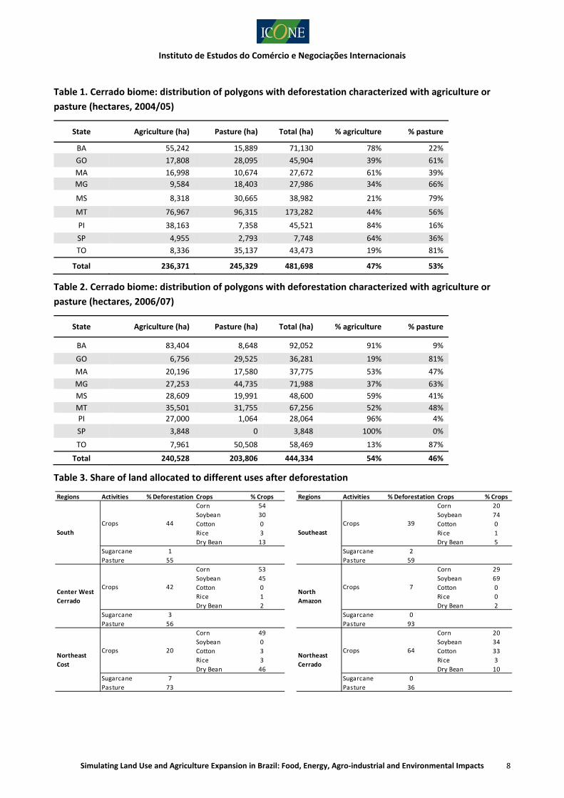
The quantification of the expansion of crops and pastures over native vegetation as presented in Table 3 was calculated in two steps. The first step was to establish the share of annual crops, pastures and sugarcane on the direct conversion of native vegetation (Table 1 and Table 2). The second step was to establish the share of individual crops in total conversion caused by annual crops. The shares in the second step were calculated based on the methodology proposed by Nassar et al. (2010, op. cit.; 2011b, op. cit.).
The approach proposed by Nassar et al. is an allocation methodology where the substitution of productive activities and natural vegetation by other productive activities is calculated from absolute variations observed over a determined period of time. The positive variations are allocated to the negative variations based on assumptions related to land use changes. The allocation assumptions, mainly in the case of natural vegetation substitution, were calibrated by physical data obtained from satellite imaging. The coefficients of competition and advancement of the agricultural frontier were calculated by the combination of secondary data ‐ gathered mostly from Produção Agrícola Municipal (PAM‐Municipal Agricultural Production) of the IBGE ‐ and remote sensing primary data for deforestation rates (Amazon, Atlantic Forest and Cerrado biomes) ‐ gathered from the Instituto Nacional de Pesquisas Espaciais (INPE) and the Laboratório de Processamento de Imagens e Geoprocessamento (LAPIG) of the Universidade Federal de Goiás. The calculations were performed for each IBGE micro‐region (550 approximately) and aggregated to BLUM’s 6 regions.
The approach used in Nassar et al., however, only allows the quantification of the individual contribution of agricultural activities to the conversion of native vegetation as a result of the allocation methodology. Nassar et al. used the variations in planted areas and deforestation rates to allocate positive variations over native vegetation. The approach used in this project is different and is based on observable data from remote sensing. In this project, the land uses in newly deforested areas for Amazon and Cerrado biomes were estimated with satellite imagery. The share of pastures, annual crops and sugarcane in conversion of
14 A detailed description of all data included in BLUM supply and demand module is described in the section 7.3. of the submission of this project to Auxílio à Pesquisa/Projeto Temático. 15 Sparovek, G.; Barreto, A.; Klug, I.; Papp, L.; Lino, J. 2010b A revisão do Código Florestal brasileiro. Novos Estudos, 88, 181‐205.

Instituto de Estudos do Comércio e Negociações Internacionais
Simulating Land Use and Agriculture Expansion in Brazil: Food, Energy, Agro‐industrial and Environmental Impacts 7
native vegetation (first step), therefore, was established with observable data from satellite imagery16. Due to limitations regarding the methodologies to interpret satellite images visually, it was not possible to separate annual crops. Such limitation gave rise to the need to take the second step: to split land use class annual crops into individual crops.
The expansion of crops and pastures over native vegetation in the Amazon biome was estimated through data from the Soybean Moratorium initiative (Rudorff et al., 2011)17. Excluding non productive uses such as burning and natural forest recovery in newly deforested areas, the observed shares of pastures and crops for the year 2007/08 were 93% and 7% respectively.. This share was used in BLUM Northern Amazon region (Table 3).
In the case of the Cerrado biome, a specific methodology was developed by LAPIG18 and its results were incorporated in this project. LAPIG is responsible for the Sistema Integrado de Alerta de Desmatamentos (SIAD), which monitors deforestation in the Cerrado biome (comprising the states of Goiás, Distrito Federal, Bahia, Tocantins, Mato Grosso, Mato Grosso do Sul, Maranhão, Piauí, São Paulo and Minas Gerais) on a yearly basis. Detailed descriptions of the methodology used for detection of deforestation can be found in Ferreira et al. (2007), Ferreira et al. (2009, op. cit.) and Rocha et al. (2010)19. The methodology developed by LAPIG for this project can be found in Ferreira et al. (2011, op. cit.).
The main purpose of LAPIG’s research was to assess the first occupation of the land once it had been cleared. Three classes of productive uses were defined: annual crops (agriculture), pastures and sugarcane. The deforested polygons analyzed for this project refer to the following period: 2004/05 and 2006/07. The results of this research that are relevant to this project are described in Table 1 and Table 2. For the 2004/05 period, newly cleared Cerrado occupation share was 47% with agriculture and 53% with pastures, while in 2006/07 the share of agriculture increased to 54%. The distribution is not homogeneous among states.
The main contribution of LAPIG to this project was to evaluate the advancement of annual crops and pastures over the Cerrado. A similar analysis was developed for sugarcane but it was based on CANASAT maps (Rudorff et al., 2010 20) rather than SIAD maps. The share of sugarcane in the conversion of native vegetation presented in Table 3, therefore, is based on CANASAT maps.
16 Given that the evaluation of the occupation of newly deforested areas by agricultural uses through satellite imagery is available only for Amazon and Cerrados biomes (comprising BLUM regions Southeast, Center‐West Cerrados, Northeast Cerrados and Nothern Amazon), direct advancement of agricultural activities over native vegetation for BLUM regions South and Northeast Coast was fully accessed based on Nassar et al. (2010, 2011b). 17 Rudorff, B. F. T.; Adami, M.; Aguiar, D. A.; Moreira, M. A.; Mello, M. P.; Fabiani, L.; Amaral, D. F.; Pires, B. M. 2011 The Soy Moratorium in the Amazon Biome Monitored by Remote Sensing Images. Remote Sensing, 3(1), 185‐202 (doi:10.3390/rs3010185). 18 This project funded LAPIG work. The main results of the research can be found in Ferreira et al. (op. cit.). 19 Ferreira, N.C.; Ferreira Junior, L.G.; Huete, A.R.; Ferreira, M.E. An operational deforestation mapping system using MODIS data and spatial context analysis. International Journal of Remote Sensing, v. 28, p. 47‐62, 2007. Ferreira, M.E.; Garcia, F.N.; Fernandes, G. Validação do Sistema Integrado de Alerta de Desmatamentos para a região de savanas no Brasil. In: Simpósio Brasileiro de Sensoriamento Remoto, 2009, Natal. Anais do XIV SBSR. São José dos Campos: INPE, 2009. Rocha, G.F.; Ferreira, N.C.; Ferreira JR., L.G.; Ferreira, M.E. Deteção de desmatamentos no bioma Cerrado entre 2002 e 2009: padrões, tendências e impactos. Revista Brasileira de Cartografia, 2010 (to be published). 20 Rudorff, B.F.T; Aguiar, D. A.; Silva, W. F.; Sugawara, L. M.; Adami, M; Moreira, M. A. 2010 Studies on the Rapid Expansion of Sugarcane for Ethanol Production in São Paulo State (Brazil) Using Landsat Data. Remote Sensing, 2, 1057‐1076.
Instituto de Estudos do Comércio e Negociações Internacionais
Simulating Land Use and Agriculture Expansion in Brazil: Food, Energy, Agro‐industrial and Environmental Impacts 8
Table 1. Cerrado biome: distribution of polygons with deforestation characterized with agriculture or
pasture (hectares, 2004/05)
State Agriculture (ha) Pasture (ha) Total (ha) % agriculture % pasture
BA 55,242 15,889 71,130 78% 22%
GO 17,808 28,095 45,904 39% 61%
MA 16,998 10,674 27,672 61% 39%
MG 9,584 18,403 27,986 34% 66%
MS 8,318 30,665 38,982 21% 79%
MT 76,967 96,315 173,282 44% 56%
PI 38,163 7,358 45,521 84% 16%
SP 4,955 2,793 7,748 64% 36%
TO 8,336 35,137 43,473 19% 81%
Total 236,371 245,329 481,698 47% 53%
Table 2. Cerrado biome: distribution of polygons with deforestation characterized with agriculture or
pasture (hectares, 2006/07)
State Agriculture (ha) Pasture (ha) Total (ha) % agriculture % pasture
BA 83,404 8,648 92,052 91% 9%
GO 6,756 29,525 36,281 19% 81%
MA 20,196 17,580 37,775 53% 47%
MG 27,253 44,735 71,988 37% 63%
MS 28,609 19,991 48,600 59% 41%
MT 35,501 31,755 67,256 52% 48%
PI 27,000 1,064 28,064 96% 4%
SP 3,848 0 3,848 100% 0%
TO 7,961 50,508 58,469 13% 87%
Total 240,528 203,806 444,334 54% 46%
Table 3. Share of land allocated to different uses after deforestation
Regions Activities % Deforestation Crops % Crops Regions Activities % Deforestation Crops % Crops
Corn 54 Corn 20
Soybean 30 Soybean 74
Cotton 0 Cotton 0
Rice 3 Rice 1
Dry Bean 13 Dry Bean 5
Sugarcane 1 Sugarcane 2
Pasture 55 Pasture 59
Corn 53 Corn 29
Soybean 45 Soybean 69
Cotton 0 Cotton 0
Rice 1 Rice 0
Dry Bean 2 Dry Bean 2
Sugarcane 3 Sugarcane 0
Pasture 56 Pasture 93
Corn 49 Corn 20
Soybean 0 Soybean 34
Cotton 3 Cotton 33
Rice 3 Rice 3
Dry Bean 46 Dry Bean 10
Sugarcane 7 Sugarcane 0
Pasture 73 Pasture 36
39
Crops 7
Crops 64Northeast
Cost
Crops 20Northeast
Cerrado
44
North
Amazon
Crops
South Southeast
Center West
Cerrado
Crops 42
Crops
Instituto de Estudos do Comércio e Negociações Internacionais
Simulating Land Use and Agriculture Expansion in Brazil: Food, Energy, Agro‐industrial and Environmental Impacts 9
3.1.2. Economic Data
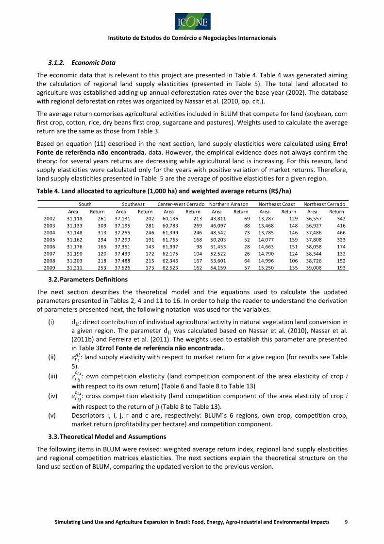
The economic data that is relevant to this project are presented in Table 4. Table 4 was generated aiming the calculation of regional land supply elasticities (presented in Table 5). The total land allocated to agriculture was established adding up annual deforestation rates over the base year (2002). The database with regional deforestation rates was organized by Nassar et al. (2010, op. cit.).
The average return comprises agricultural activities included in BLUM that compete for land (soybean, corn first crop, cotton, rice, dry beans first crop, sugarcane and pastures). Weights used to calculate the average return are the same as those from Table 3.
Based on equation (11) described in the next section, land supply elasticities were calculated using Erro! Fonte de referência não encontrada. data. However, the empirical evidence does not always confirm the theory: for several years returns are decreasing while agricultural land is increasing. For this reason, land supply elasticities were calculated only for the years with positive variation of market returns. Therefore, land supply elasticities presented in Table 5 are the average of positive elasticities for a given region.
Table 4. Land allocated to agriculture (1,000 ha) and weighted average returns (R$/ha)
3.2. Parameters Definitions
The next section describes the theoretical model and the equations used to calculate the updated parameters presented in Tables 2, 4 and 11 to 16. In order to help the reader to understand the derivation of parameters presented next, the following notation was used for the variables:
(i) d : direct contribution of individual agricultural activity in natural vegetation land conversion in a given region. The parameter d was calculated based on Nassar et al. (2010), Nassar et al. (2011b) and Ferreira et al. (2011). The weights used to establish this parameter are presented in Table 3Erro! Fonte de referência não encontrada..
(ii) : land supply elasticity with respect to market return for a give region (for results see Table
5).
(iii) , : own competition elasticity (land competition component of the area elasticity of crop i
with respect to its own return) (Table 6 and Table 8 to Table 13)
(iv) , : cross competition elasticity (land competition component of the area elasticity of crop i
with respect to the return of j) (Table 8 to Table 13). (v) Descriptors l, i, j, r and c are, respectively: BLUM´s 6 regions, own crop, competition crop,
market return (profitability per hectare) and competition component.
3.3. Theoretical Model and Assumptions
The following items in BLUM were revised: weighted average return index, regional land supply elasticities and regional competition matrices elasticities. The next sections explain the theoretical structure on the land use section of BLUM, comparing the updated version to the previous version.
Area Return Area Return Area Return Area Return Area Return Area Return
2002 31,118 261 37,131 202 60,136 213 43,811 69 13,287 129 36,557 342
2003 31,133 309 37,195 281 60,783 269 46,097 88 13,468 148 36,927 416
2004 31,148 313 37,255 246 61,399 246 48,542 73 13,785 146 37,486 466
2005 31,162 294 37,299 191 61,765 168 50,203 52 14,077 159 37,808 323
2006 31,176 165 37,351 143 61,997 98 51,453 28 14,663 151 38,058 174
2007 31,190 120 37,439 172 62,175 104 52,522 26 14,790 124 38,344 132
2008 31,203 218 37,488 215 62,346 167 53,601 64 14,996 106 38,726 152
2009 31,211 253 37,526 173 62,523 162 54,159 57 15,250 135 39,008 193
Northern Amazon Northeast Coast Northeast CerradoSouth Southeast Center‐West Cerrado
Instituto de Estudos do Comércio e Negociações Internacionais
Simulating Land Use and Agriculture Expansion in Brazil: Food, Energy, Agro‐industrial and Environmental Impacts 10
3.3.1. Previous version of the model
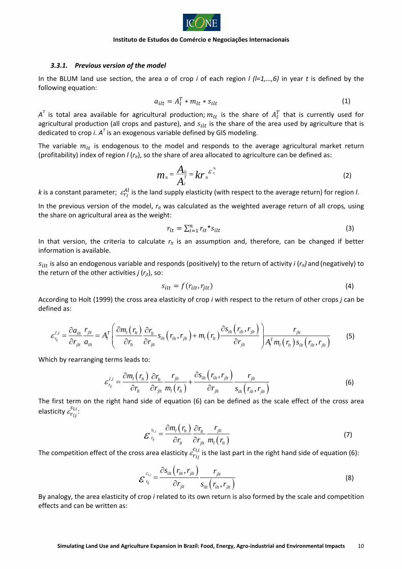
In the BLUM land use section, the area a of crop i of each region l (l=1,…,6) in year t is defined by the following equation:
∗ ∗ (1)
AT is total area available for agricultural production; is the share of that is currently used for agricultural production (all crops and pasture), and is the share of the area used by agriculture that is dedicated to crop i. AT is an exogenous variable defined by GIS modeling.
The variable is endogenous to the model and responds to the average agricultural market return (profitability) index of region l (rlt), so the share of area allocated to agriculture can be defined as:
Alrllt
Tlt lt
l
Am krA
(2)
k is a constant parameter; is the land supply elasticity (with respect to the average return) for region l.
In the previous version of the model, rlt was calculated as the weighted average return of all crops, using the share on agricultural area as the weight:
∑ * (3)
In that version, the criteria to calculate rlt is an assumption and, therefore, can be changed if better information is available.
is also an endogenous variable and responds (positively) to the return of activity i (rit) and (negatively) to the return of the other activities j (rjt), so:
, (4)
According to Holt (1999) the cross area elasticity of crop i with respect to the return of other crops j can be defined as:
,,
,,lj
ilt ilt jltjlt jltl ltl i Tilt ltr l ilt ilt jlt l lt T
jlt ilt lt jlt jlt l l lt ilt ilt jlt
s r rr rm ra rA s r r m r
r a r r r A m r s r r
(5)
Which by rearranging terms leads to:
,,
,lj
ilt ilt jltjlt jltl ltl i ltr
lt jlt l lt jlt ilt ilt jlt
s r rr rm r r
r r m r r s r r
(6)
The first term on the right hand side of equation (6) can be defined as the scale effect of the cross area
elasticity , :
,l i
lj
s jltl lt ltr
lt jlt l lt
rm r r
r r m r
(7)
The competition effect of the cross area elasticity , is the last part in the right hand side of equation (6):
,,
,l i
lj
c ilt ilt jlt jlt
rjlt ilt ilt jlt
s r r r
r s r r
(8)
By analogy, the area elasticity of crop i related to its own return is also formed by the scale and competition effects and can be written as:

Instituto de Estudos do Comércio e Negociações Internacionais
Simulating Land Use and Agriculture Expansion in Brazil: Food, Energy, Agro‐industrial and Environmental Impacts 11
, ,,,
,l i l i
li li li
s cilt ilt jltl ltl i lt ilt iltr r r
lt ilt l lt ilt ilt ilt jlt
s r rm r r r r
r r m r r s r r
(9)
Where , is the scale effect and , is the land competition component of the area elasticity of crop i with
respect to its own return.
The land competition component can then be calculated as:
, ,,l i l i
li lt li
c l i s
r r r (10)
The link between the regional land supply elasticity ( ) and the scale effect of each activity ( , can be
observed. The land supply elasticity can be defined as:
l
l
A l lr
l l
m rr m
(11)
And rearranging:
l
l
A
r ll
ll
mmr r
(12)
The elasticity with respect to the variation in return of a given crop i in region l is:
,l i
li
s l l lir
l li l
m r rr r m
(13)
Which from equation (12) and with some calculation can be rewritten as:
,l i l
li l
s A l lr r
lili
r rr r
(13)
From equation (3), equation (13) can be rewritten as:
,l i l
li l
s A lr r ilt
li
rs r (14)
Using equation (14), if the land supply elasticity is known, the scale effect of activity i can be easily
calculated. As a result, the vector containing all land competition component elasticities , represents the
diagonal of the competition matrix (one for each region l). Along with other restrictions (such as homogeneity, adding up, symmetry and negative cross elasticities) the diagonal terms are then used to obtain the cross elasticities in the competition matrix, as represented in equation (8).
3.3.2. Improvements on BLUM elasticities
Considering data available, the weighted average returns related to area seemed to be the best approach to determine agricultural land expansion. However, deeper literature review showed that some activities (notably pasture and some grains) are especially related to agricultural expansion (scale effect), while others tend to compete only with other activities21. This means that the land use dynamics and the
21 Part of the literature review includes: Ferreira et al. (2009, op.cit.) Ferreira et al. (2011, op.cit.) Rudorff et al. (2011, op. cit.) Morton, D. C.; Defries, R. S.; Shimabukuro, Y. E.; Anderson, L. O.; Arai, E.; Del Bon Espirito‐Santo, F.; Freitas, R.; Morisette, J. 2006 Cropland Expansion Changes Deforestation Dynamics in the Southern Brazilian Amazon. PNAS, 103, no. 39, pp 14,637‐14,641. (DOI 10.1073/pnas.0606377103)
Instituto de Estudos do Comércio e Negociações Internacionais
Simulating Land Use and Agriculture Expansion in Brazil: Food, Energy, Agro‐industrial and Environmental Impacts 12
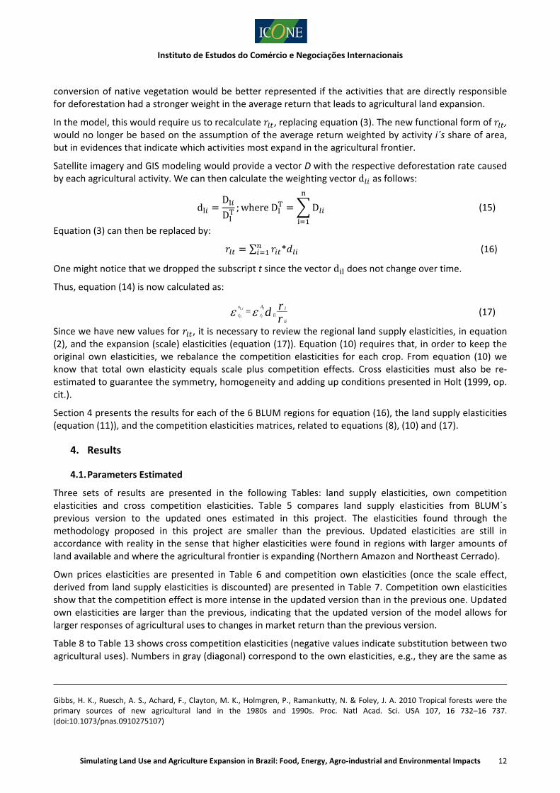
conversion of native vegetation would be better represented if the activities that are directly responsible for deforestation had a stronger weight in the average return that leads to agricultural land expansion.
In the model, this would require us to recalculate , replacing equation (3). The new functional form of , would no longer be based on the assumption of the average return weighted by activity i´s share of area, but in evidences that indicate which activities most expand in the agricultural frontier.
Satellite imagery and GIS modeling would provide a vector D with the respective deforestation rate caused by each agricultural activity. We can then calculate the weighting vector d as follows:
dD
D;where D D (15)
Equation (3) can then be replaced by:
∑ * (16)
One might notice that we dropped the subscript t since the vector d does not change over time.
Thus, equation (14) is now calculated as:
,l i l
li l
s A lr r li
li
rd r (17)
Since we have new values for , it is necessary to review the regional land supply elasticities, in equation (2), and the expansion (scale) elasticities (equation (17)). Equation (10) requires that, in order to keep the original own elasticities, we rebalance the competition elasticities for each crop. From equation (10) we know that total own elasticity equals scale plus competition effects. Cross elasticities must also be re‐estimated to guarantee the symmetry, homogeneity and adding up conditions presented in Holt (1999, op. cit.).
Section 4 presents the results for each of the 6 BLUM regions for equation (16), the land supply elasticities (equation (11)), and the competition elasticities matrices, related to equations (8), (10) and (17).
4. Results
4.1. Parameters Estimated
Three sets of results are presented in the following Tables: land supply elasticities, own competition elasticities and cross competition elasticities. Table 5 compares land supply elasticities from BLUM´s previous version to the updated ones estimated in this project. The elasticities found through the methodology proposed in this project are smaller than the previous. Updated elasticities are still in accordance with reality in the sense that higher elasticities were found in regions with larger amounts of land available and where the agricultural frontier is expanding (Northern Amazon and Northeast Cerrado).
Own prices elasticities are presented in Table 6 and competition own elasticities (once the scale effect, derived from land supply elasticities is discounted) are presented in Table 7. Competition own elasticities show that the competition effect is more intense in the updated version than in the previous one. Updated own elasticities are larger than the previous, indicating that the updated version of the model allows for larger responses of agricultural uses to changes in market return than the previous version.
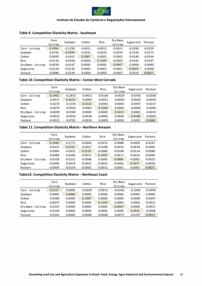
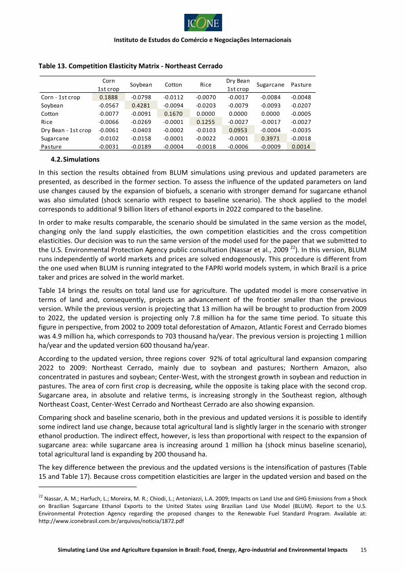
Table 8 to Table 13 shows cross competition elasticities (negative values indicate substitution between two agricultural uses). Numbers in gray (diagonal) correspond to the own elasticities, e.g., they are the same as
Gibbs, H. K., Ruesch, A. S., Achard, F., Clayton, M. K., Holmgren, P., Ramankutty, N. & Foley, J. A. 2010 Tropical forests were the primary sources of new agricultural land in the 1980s and 1990s. Proc. Natl Acad. Sci. USA 107, 16 732–16 737. (doi:10.1073/pnas.0910275107)

Instituto de Estudos do Comércio e Negociações Internacionais
Simulating Land Use and Agriculture Expansion in Brazil: Food, Energy, Agro‐industrial and Environmental Impacts 13
those in Table 7. Crops “i” is in the rows and crops “j” in the columns, which means that for the South region a variation of 10% in the return of soybean will lead soybean to displace 0.572% of corn area.
Table 5. Land Supply Elasticities ( )
Regions Previous Version Updated Version
South 0.057 0.002
Southeast 0.067 0.007
Center West Cerrado 0.180 0.031
Northern Amazon 0.250 0.103
Northeast Coast 0.010 0.056
Northeast Cerrado 0.100 0.066
Table 6. Own elasticities
South Southeast Center West Cerrado
North Amazon Costal
Northeast Northeast Cerrado
Corn ‐ 1st crop 0.18 0.20 0.20 0.20 0.22 0.19 Soybean 0.43 0.43 0.48 0.45 0.00 0.44 Cotton 0.21 0.21 0.25 0.25 0.20 0.22 Rice 0.15 0.12 0.13 0.15 0.13 0.13 Dry Bean ‐ 1st crop
0.09 0.10 0.10 0.09 0.10 0.10
Sugarcane 0.40 0.40 0.43 0.20 0.39 0.40 Pasture 0.03 0.05 0.11 0.24 0.01 0.07
Table 7. Competition effects (from own elasticities) ( , )
South Southeast Center‐West Cerrado
North Amazon Coastal Northeast Northeast Cerrado
Previous Updated Previous Updated Previous Updated Previous Updated Previous Updated Previous Updated
Corn ‐ 1st crop
0.18 0.18 0.20 0.20 0.20 0.20 0.19 0.19 0.22 0.22 0.18 0.19
Soybean 0.40 0.43 0.43 0.43 0.39 0.47 0.40 0.43 0.00 0.00 0.42 0.43 Cotton 0.21 0.21 0.21 0.21 0.25 0.25 0.25 0.25 0.20 0.20 0.20 0.17 Rice 0.15 0.15 0.12 0.12 0.12 0.13 0.13 0.15 0.13 0.13 0.11 0.13 Dry Bean ‐ 1st crop
0.09 0.09 0.09 0.09 0.10 0.10 0.08 0.09 0.10 0.10 0.09 0.10
Sugarcane 0.39 0.40 0.36 0.40 0.40 0.42 0.19 0.20 0.38 0.34 0.39 0.40 Pasture 0.02 0.03 0.04 0.05 0.05 0.11 0.08 0.17 0.01 0.01 0.05 0.07
Table 8. Competition Elasticity Matrix – South ( , and , )
Corn
1st cropSoybean Cotton Rice
Dry Bean
1st cropSugarcane Pasture
Corn 1st crop 0.1838 ‐0.2695 ‐0.0003 ‐0.0095 ‐0.0023 ‐0.0104 ‐0.0058
Soybean ‐0.0572 0.4334 ‐0.0002 ‐0.0052 ‐0.0013 ‐0.0064 ‐0.0261
Cotton ‐0.0164 ‐0.0540 0.2087 ‐0.0015 ‐0.0009 ‐0.0055 ‐0.0093
Rice ‐0.0102 ‐0.0265 0.0000 0.1529 ‐0.0025 ‐0.0060 ‐0.0049
Dry Bean 1st crop ‐0.0188 ‐0.0483 ‐0.0001 ‐0.0185 0.0914 ‐0.0031 ‐0.0104
Sugarcane ‐0.0106 ‐0.0307 ‐0.0001 ‐0.0057 ‐0.0004 0.3998 ‐0.0047
Pasture ‐0.0076 ‐0.1603 ‐0.0002 ‐0.0059 ‐0.0017 ‐0.0061 0.0154
Instituto de Estudos do Comércio e Negociações Internacionais
Simulating Land Use and Agriculture Expansion in Brazil: Food, Energy, Agro‐industrial and Environmental Impacts 14
Table 9. Competition Elasticity Matrix ‐ Southeast
Table 10. Competition Elasticity Matrix – Center‐West Cerrado
Table 11. Competition Elasticity Matrix – Northern Amazon
Table12. Competition Elasticity Matrix – Northeast Coast
Corn
1st cropSoybean Cotton Rice
Dry Bean
1st cropSugarcane Pasture
Corn ‐ 1st crop 0.1994 ‐0.1299 ‐0.0011 ‐0.0012 ‐0.0011 ‐0.2038 ‐0.0259
Soybean ‐0.0782 0.4299 ‐0.0031 ‐0.0024 ‐0.0034 ‐0.1249 ‐0.0273
Cotton ‐0.0093 ‐0.0437 0.2087 ‐0.0001 ‐0.0001 ‐0.0180 ‐0.0146
Rice ‐0.0139 ‐0.0458 ‐0.0002 0.1200 ‐0.0002 ‐0.0181 ‐0.0107
Dry Bean ‐ 1st crop ‐0.0038 ‐0.0187 0.0000 0.0000 0.0947 ‐0.0069 ‐0.0080
Sugarcane ‐0.0134 ‐0.0136 ‐0.0001 ‐0.0001 ‐0.0001 0.4029 ‐0.0068
Pasture ‐0.0080 ‐0.0140 ‐0.0005 ‐0.0003 ‐0.0007 ‐0.0319 0.0047
Corn
1st cropSoybean Cotton Rice
Dry Bean
1st cropSugarcane Pasture
Corn ‐ 1st crop 0.1962 ‐0.2855 ‐0.0452 ‐0.0106 ‐0.0024 ‐0.0783 ‐0.0308
Soybean ‐0.0071 0.4674 ‐0.0064 ‐0.0021 ‐0.0003 ‐0.0049 ‐0.0459
Cotton ‐0.0274 ‐0.1559 0.2532 ‐0.0001 0.0000 ‐0.0597 ‐0.0157
Rice ‐0.0070 ‐0.0563 ‐0.0001 0.1266 0.0000 ‐0.0009 ‐0.0093
Dry Bean ‐ 1st crop ‐0.0038 ‐0.0189 0.0000 0.0000 0.1011 0.0000 ‐0.0019
Sugarcane ‐0.0022 ‐0.0056 ‐0.0028 0.0000 0.0000 0.4168 ‐0.0069
Pasture ‐0.0012 ‐0.0701 ‐0.0010 ‐0.0005 0.0000 ‐0.0092 0.0084
Corn
1st cropSoybean Cotton Rice
Dry Bean
1st cropSugarcane Pasture
Corn ‐ 1st crop 0.1944 ‐0.2771 ‐0.0046 ‐0.0253 ‐0.0088 ‐0.0094 ‐0.0237
Soybean ‐0.0323 0.4252 ‐0.0027 ‐0.0188 ‐0.0022 ‐0.0018 ‐0.0460
Cotton ‐0.0090 ‐0.0452 0.2519 ‐0.0084 ‐0.0108 ‐0.0124 ‐0.0088
Rice ‐0.0089 ‐0.0569 ‐0.0015 0.1459 ‐0.0017 ‐0.0023 ‐0.0096
Dry Bean ‐ 1st crop ‐0.0108 ‐0.0231 ‐0.0068 ‐0.0060 0.0884 ‐0.0005 ‐0.0025
Sugarcane ‐0.0046 ‐0.0076 ‐0.0031 ‐0.0031 ‐0.0002 0.1977 ‐0.0028
Pasture ‐0.0009 ‐0.0154 ‐0.0002 ‐0.0011 ‐0.0001 ‐0.0002 0.0027
Corn
1st cropSoybean Cotton Rice
Dry Bean
1st cropSugarcane Pasture
Corn ‐ 1st crop 0.2157 0.0000 ‐0.0029 ‐0.0015 ‐0.0350 ‐0.1000 ‐0.0099
Soybean 0.0000 0.0000 0.0000 0.0000 0.0000 0.0000 0.0000
Cotton ‐0.0580 0.0000 0.1997 0.0000 0.0000 ‐0.0080 ‐0.0047
Rice ‐0.0075 0.0000 0.0000 0.1250 ‐0.0001 ‐0.0001 ‐0.0011
Dry Bean ‐ 1st crop ‐0.0245 0.0000 0.0000 0.0000 0.0967 0.0000 ‐0.0021
Sugarcane ‐0.0104 0.0000 0.0000 0.0000 0.0000 0.3431 ‐0.0008
Pasture ‐0.0242 0.0000 ‐0.0006 ‐0.0006 ‐0.0073 ‐0.0197 0.0017
Instituto de Estudos do Comércio e Negociações Internacionais
Simulating Land Use and Agriculture Expansion in Brazil: Food, Energy, Agro‐industrial and Environmental Impacts 15
Table 13. Competition Elasticity Matrix ‐ Northeast Cerrado
4.2. Simulations
In this section the results obtained from BLUM simulations using previous and updated parameters are presented, as described in the former section. To assess the influence of the updated parameters on land use changes caused by the expansion of biofuels, a scenario with stronger demand for sugarcane ethanol was also simulated (shock scenario with respect to baseline scenario). The shock applied to the model corresponds to additional 9 billion liters of ethanol exports in 2022 compared to the baseline.
In order to make results comparable, the scenario should be simulated in the same version as the model, changing only the land supply elasticities, the own competition elasticities and the cross competition elasticities. Our decision was to run the same version of the model used for the paper that we submitted to the U.S. Environmental Protection Agency public consultation (Nassar et al., 2009 22). In this version, BLUM runs independently of world markets and prices are solved endogenously. This procedure is different from the one used when BLUM is running integrated to the FAPRI world models system, in which Brazil is a price taker and prices are solved in the world market.
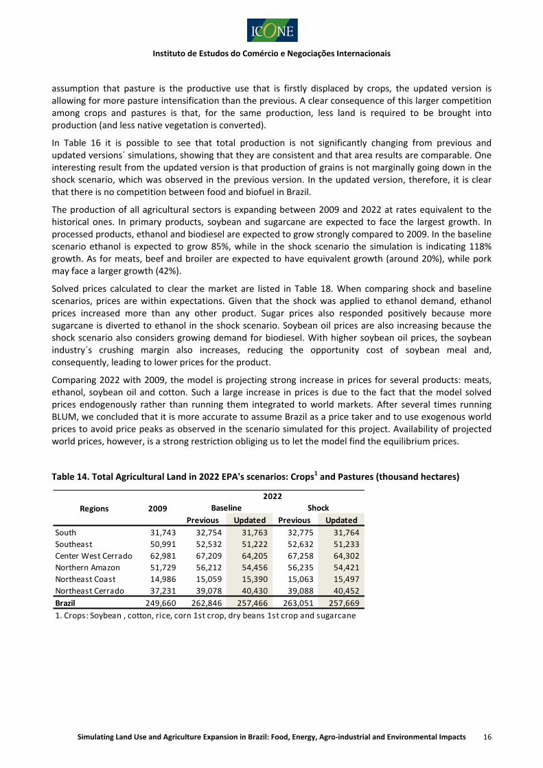
Table 14 brings the results on total land use for agriculture. The updated model is more conservative in terms of land and, consequently, projects an advancement of the frontier smaller than the previous version. While the previous version is projecting that 13 million ha will be brought to production from 2009 to 2022, the updated version is projecting only 7.8 million ha for the same time period. To situate this figure in perspective, from 2002 to 2009 total deforestation of Amazon, Atlantic Forest and Cerrado biomes was 4.9 million ha, which corresponds to 703 thousand ha/year. The previous version is projecting 1 million ha/year and the updated version 600 thousand ha/year.
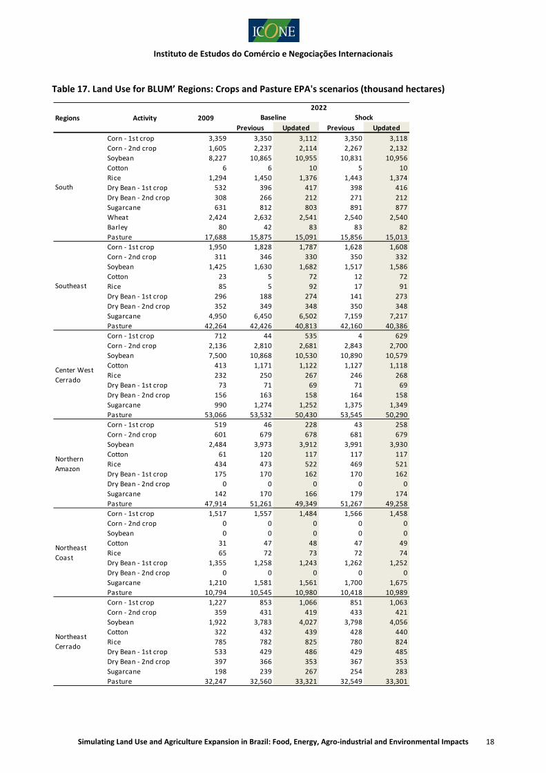
According to the updated version, three regions cover 92% of total agricultural land expansion comparing 2022 to 2009: Northeast Cerrado, mainly due to soybean and pastures; Northern Amazon, also concentrated in pastures and soybean; Center‐West, with the strongest growth in soybean and reduction in pastures. The area of corn first crop is decreasing, while the opposite is taking place with the second crop. Sugarcane area, in absolute and relative terms, is increasing strongly in the Southeast region, although Northeast Coast, Center‐West Cerrado and Northeast Cerrado are also showing expansion.
Comparing shock and baseline scenario, both in the previous and updated versions it is possible to identify some indirect land use change, because total agricultural land is slightly larger in the scenario with stronger ethanol production. The indirect effect, however, is less than proportional with respect to the expansion of sugarcane area: while sugarcane area is increasing around 1 million ha (shock minus baseline scenario), total agricultural land is expanding by 200 thousand ha.
The key difference between the previous and the updated versions is the intensification of pastures (Table 15 and Table 17). Because cross competition elasticities are larger in the updated version and based on the
22 Nassar, A. M.; Harfuch, L.; Moreira, M. R.; Chiodi, L.; Antoniazzi, L.A. 2009; Impacts on Land Use and GHG Emissions from a Shock on Brazilian Sugarcane Ethanol Exports to the United States using Brazilian Land Use Model (BLUM). Report to the U.S. Environmental Protection Agency regarding the proposed changes to the Renewable Fuel Standard Program. Available at: http://www.iconebrasil.com.br/arquivos/noticia/1872.pdf
Corn
1st cropSoybean Cotton Rice
Dry Bean
1st cropSugarcane Pasture
Corn ‐ 1st crop 0.1888 ‐0.0798 ‐0.0112 ‐0.0070 ‐0.0017 ‐0.0084 ‐0.0048
Soybean ‐0.0567 0.4281 ‐0.0094 ‐0.0203 ‐0.0079 ‐0.0093 ‐0.0207
Cotton ‐0.0077 ‐0.0091 0.1670 0.0000 0.0000 0.0000 ‐0.0005
Rice ‐0.0066 ‐0.0269 ‐0.0001 0.1255 ‐0.0027 ‐0.0017 ‐0.0027
Dry Bean ‐ 1st crop ‐0.0061 ‐0.0403 ‐0.0002 ‐0.0103 0.0953 ‐0.0004 ‐0.0035
Sugarcane ‐0.0102 ‐0.0158 ‐0.0001 ‐0.0022 ‐0.0001 0.3971 ‐0.0018
Pasture ‐0.0031 ‐0.0189 ‐0.0004 ‐0.0018 ‐0.0006 ‐0.0009 0.0014
Instituto de Estudos do Comércio e Negociações Internacionais
Simulating Land Use and Agriculture Expansion in Brazil: Food, Energy, Agro‐industrial and Environmental Impacts 16
assumption that pasture is the productive use that is firstly displaced by crops, the updated version is allowing for more pasture intensification than the previous. A clear consequence of this larger competition among crops and pastures is that, for the same production, less land is required to be brought into production (and less native vegetation is converted).
In Table 16 it is possible to see that total production is not significantly changing from previous and updated versions´ simulations, showing that they are consistent and that area results are comparable. One interesting result from the updated version is that production of grains is not marginally going down in the shock scenario, which was observed in the previous version. In the updated version, therefore, it is clear that there is no competition between food and biofuel in Brazil.
The production of all agricultural sectors is expanding between 2009 and 2022 at rates equivalent to the historical ones. In primary products, soybean and sugarcane are expected to face the largest growth. In processed products, ethanol and biodiesel are expected to grow strongly compared to 2009. In the baseline scenario ethanol is expected to grow 85%, while in the shock scenario the simulation is indicating 118% growth. As for meats, beef and broiler are expected to have equivalent growth (around 20%), while pork may face a larger growth (42%).
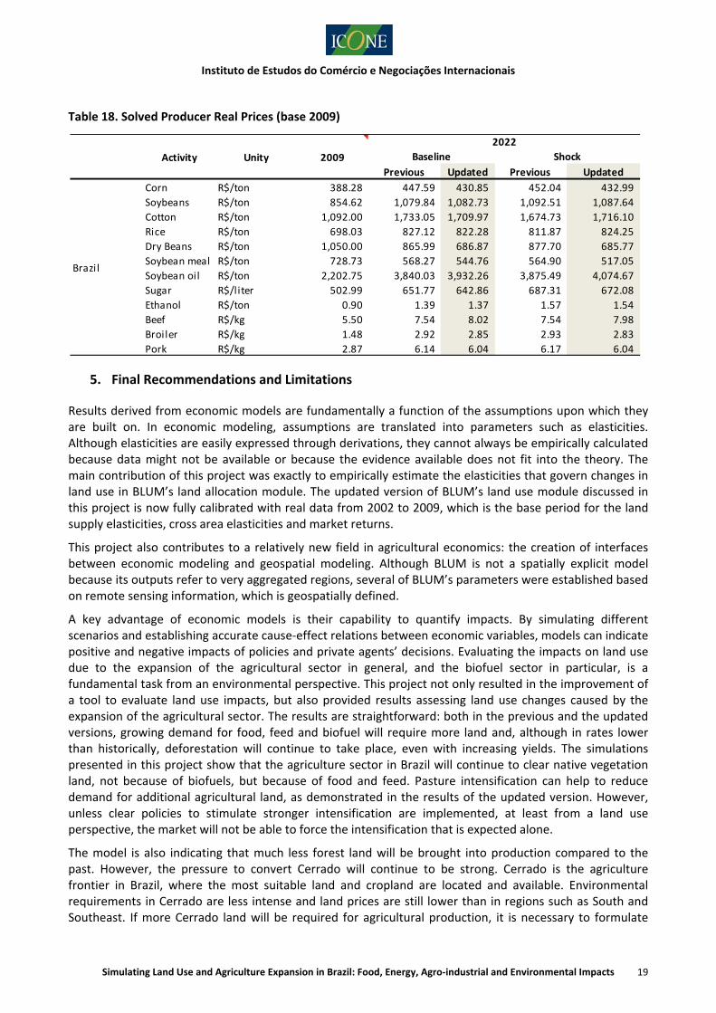
Solved prices calculated to clear the market are listed in Table 18. When comparing shock and baseline scenarios, prices are within expectations. Given that the shock was applied to ethanol demand, ethanol prices increased more than any other product. Sugar prices also responded positively because more sugarcane is diverted to ethanol in the shock scenario. Soybean oil prices are also increasing because the shock scenario also considers growing demand for biodiesel. With higher soybean oil prices, the soybean industry´s crushing margin also increases, reducing the opportunity cost of soybean meal and, consequently, leading to lower prices for the product.
Comparing 2022 with 2009, the model is projecting strong increase in prices for several products: meats, ethanol, soybean oil and cotton. Such a large increase in prices is due to the fact that the model solved prices endogenously rather than running them integrated to world markets. After several times running BLUM, we concluded that it is more accurate to assume Brazil as a price taker and to use exogenous world prices to avoid price peaks as observed in the scenario simulated for this project. Availability of projected world prices, however, is a strong restriction obliging us to let the model find the equilibrium prices.
Table 14. Total Agricultural Land in 2022 EPA's scenarios: Crops1 and Pastures (thousand hectares)
Previous Updated Previous Updated
South 31,743 32,754 31,763 32,775 31,764
Southeast 50,991 52,532 51,222 52,632 51,233
Center West Cerrado 62,981 67,209 64,205 67,258 64,302
Northern Amazon 51,729 56,212 54,456 56,235 54,421
Northeast Coast 14,986 15,059 15,390 15,063 15,497
Northeast Cerrado 37,231 39,078 40,430 39,088 40,452
Brazil 249,660 262,846 257,466 263,051 257,669
1. Crops: Soybean , cotton, rice, corn 1st crop, dry beans 1st crop and sugarcane
Regions 2009
2022
ShockBaseline

Instituto de Estudos do Comércio e Negociações Internacionais
Simulating Land Use and Agriculture Expansion in Brazil: Food, Energy, Agro‐industrial and Environmental Impacts 17
Table 15. Land Use for Brazil: Crops and Pasture EPA's scenarios (thousand hectares)
Table 16. Crops and Pasture: Production in 2022 EPA's scenarios (thousand tons)
Previous Updated Previous Updated
Corn ‐ 1st crop 9,285 7,678 8,214 7,442 8,134
Corn ‐ 2nd crop 5,011 6,503 6,223 6,573 6,264
Soybean 21,557 31,118 31,105 31,026 31,108
Cotton 856 1,782 1,808 1,736 1,806
Rice 2,894 3,033 3,155 3,025 3,153
Dry Bean ‐ 1st crop 2,963 2,511 2,651 2,470 2,657
Dry Bean ‐ 2nd crop 1,212 1,145 1,071 1,151 1,072
Sugarcane 8,120 10,525 10,551 11,558 11,575
Wheat 2,424 2,632 2,541 2,540 2,540
Barley 80 42 83 83 82
Pasture 203,973 206,199 199,982 205,794 199,237
Regions Activity
Brazil
2022
Baseline Shock2009
Previous Updated Previous Updated
Corn ‐ 1st crop 33,129 35,260 37,221 33,826 36,859
Corn ‐ 2nd crop 17,239 31,391 29,259 31,921 29,610
Soybean 57,635 98,174 98,152 97,943 98,220
Cotton 1,244 3,361 3,383 3,275 3,381
Rice 12,519 14,683 14,758 14,638 14,746
Dry Bean ‐ 1st crop 2,165 2,311 2,526 2,223 2,527
Dry Bean ‐ 2nd crop 1,570 2,136 1,984 2,150 1,985
Sugarcane 639,356 969,046 972,087 1,082,989 1,084,699
Wheat 6,031 6,089 6,195 6,087 6,193
Barley 235 150 298 147 295
Biodiesel 1,765 3,167 3,167 3,167 3,167
Soybean oil 6,250 6,601 6,586 6,554 6,596
Soybean meal 24,300 25,666 25,606 25,483 25,647
Sugar 33,096 43,845 43,879 43,767 43,843
Ethanol 29,048 53,646 53,821 63,188 63,229
Beef 10,211 12,493 12,336 12,493 12,339
Pork 3,286 4,631 4,654 4,624 4,653
Broiler 11,004 13,163 13,228 13,156 13,234
2022
Baseline Shock2009Regions Activity
Brazil
Instituto de Estudos do Comércio e Negociações Internacionais
Simulating Land Use and Agriculture Expansion in Brazil: Food, Energy, Agro‐industrial and Environmental Impacts 18
Table 17. Land Use for BLUM’ Regions: Crops and Pasture EPA's scenarios (thousand hectares)
Previous Updated Previous Updated
Corn ‐ 1st crop 3,359 3,350 3,112 3,350 3,118
Corn ‐ 2nd crop 1,605 2,237 2,114 2,267 2,132
Soybean 8,227 10,865 10,955 10,831 10,956
Cotton 6 6 10 5 10
Rice 1,294 1,450 1,376 1,443 1,374
Dry Bean ‐ 1st crop 532 396 417 398 416
Dry Bean ‐ 2nd crop 308 266 212 271 212
Sugarcane 631 812 803 891 877
Wheat 2,424 2,632 2,541 2,540 2,540
Barley 80 42 83 83 82
Pasture 17,688 15,875 15,091 15,856 15,013
Corn ‐ 1st crop 1,950 1,828 1,787 1,628 1,608
Corn ‐ 2nd crop 311 346 330 350 332
Soybean 1,425 1,630 1,682 1,517 1,586
Cotton 23 5 72 12 72
Rice 85 5 92 17 91
Dry Bean ‐ 1st crop 296 188 274 141 273
Dry Bean ‐ 2nd crop 352 349 348 350 348
Sugarcane 4,950 6,450 6,502 7,159 7,217
Pasture 42,264 42,426 40,813 42,160 40,386
Corn ‐ 1st crop 712 44 535 4 629
Corn ‐ 2nd crop 2,136 2,810 2,681 2,843 2,700
Soybean 7,500 10,868 10,530 10,890 10,579
Cotton 413 1,171 1,122 1,127 1,118
Rice 232 250 267 246 268
Dry Bean ‐ 1st crop 73 71 69 71 69
Dry Bean ‐ 2nd crop 156 163 158 164 158
Sugarcane 990 1,274 1,252 1,375 1,349
Pasture 53,066 53,532 50,430 53,545 50,290
Corn ‐ 1st crop 519 46 228 43 258
Corn ‐ 2nd crop 601 679 678 681 679
Soybean 2,484 3,973 3,912 3,991 3,930
Cotton 61 120 117 117 117
Rice 434 473 522 469 521
Dry Bean ‐ 1st crop 175 170 162 170 162
Dry Bean ‐ 2nd crop 0 0 0 0 0
Sugarcane 142 170 166 179 174
Pasture 47,914 51,261 49,349 51,267 49,258
Corn ‐ 1st crop 1,517 1,557 1,484 1,566 1,458
Corn ‐ 2nd crop 0 0 0 0 0
Soybean 0 0 0 0 0
Cotton 31 47 48 47 49
Rice 65 72 73 72 74
Dry Bean ‐ 1st crop 1,355 1,258 1,243 1,262 1,252
Dry Bean ‐ 2nd crop 0 0 0 0 0
Sugarcane 1,210 1,581 1,561 1,700 1,675
Pasture 10,794 10,545 10,980 10,418 10,989
Corn ‐ 1st crop 1,227 853 1,066 851 1,063
Corn ‐ 2nd crop 359 431 419 433 421
Soybean 1,922 3,783 4,027 3,798 4,056
Cotton 322 432 439 428 440
Rice 785 782 825 780 824
Dry Bean ‐ 1st crop 533 429 486 429 485
Dry Bean ‐ 2nd crop 397 366 353 367 353
Sugarcane 198 239 267 254 283
Pasture 32,247 32,560 33,321 32,549 33,301
Center West
Cerrado
Northern
Amazon
Northeast
Coast
Northeast
Cerrado
South
Southeast
Regions Activity
2022
Baseline Shock2009
Instituto de Estudos do Comércio e Negociações Internacionais
Simulating Land Use and Agriculture Expansion in Brazil: Food, Energy, Agro‐industrial and Environmental Impacts 19
Table 18. Solved Producer Real Prices (base 2009)
5. Final Recommendations and Limitations
Results derived from economic models are fundamentally a function of the assumptions upon which they are built on. In economic modeling, assumptions are translated into parameters such as elasticities. Although elasticities are easily expressed through derivations, they cannot always be empirically calculated because data might not be available or because the evidence available does not fit into the theory. The main contribution of this project was exactly to empirically estimate the elasticities that govern changes in land use in BLUM’s land allocation module. The updated version of BLUM’s land use module discussed in this project is now fully calibrated with real data from 2002 to 2009, which is the base period for the land supply elasticities, cross area elasticities and market returns.
This project also contributes to a relatively new field in agricultural economics: the creation of interfaces between economic modeling and geospatial modeling. Although BLUM is not a spatially explicit model because its outputs refer to very aggregated regions, several of BLUM’s parameters were established based on remote sensing information, which is geospatially defined.
A key advantage of economic models is their capability to quantify impacts. By simulating different scenarios and establishing accurate cause‐effect relations between economic variables, models can indicate positive and negative impacts of policies and private agents’ decisions. Evaluating the impacts on land use due to the expansion of the agricultural sector in general, and the biofuel sector in particular, is a fundamental task from an environmental perspective. This project not only resulted in the improvement of a tool to evaluate land use impacts, but also provided results assessing land use changes caused by the expansion of the agricultural sector. The results are straightforward: both in the previous and the updated versions, growing demand for food, feed and biofuel will require more land and, although in rates lower than historically, deforestation will continue to take place, even with increasing yields. The simulations presented in this project show that the agriculture sector in Brazil will continue to clear native vegetation land, not because of biofuels, but because of food and feed. Pasture intensification can help to reduce demand for additional agricultural land, as demonstrated in the results of the updated version. However, unless clear policies to stimulate stronger intensification are implemented, at least from a land use perspective, the market will not be able to force the intensification that is expected alone.
The model is also indicating that much less forest land will be brought into production compared to the past. However, the pressure to convert Cerrado will continue to be strong. Cerrado is the agriculture frontier in Brazil, where the most suitable land and cropland are located and available. Environmental requirements in Cerrado are less intense and land prices are still lower than in regions such as South and Southeast. If more Cerrado land will be required for agricultural production, it is necessary to formulate
Previous Updated Previous Updated
Corn R$/ton 388.28 447.59 430.85 452.04 432.99
Soybeans R$/ton 854.62 1,079.84 1,082.73 1,092.51 1,087.64
Cotton R$/ton 1,092.00 1,733.05 1,709.97 1,674.73 1,716.10
Rice R$/ton 698.03 827.12 822.28 811.87 824.25
Dry Beans R$/ton 1,050.00 865.99 686.87 877.70 685.77
Soybean meal R$/ton 728.73 568.27 544.76 564.90 517.05
Soybean oil R$/ton 2,202.75 3,840.03 3,932.26 3,875.49 4,074.67
Sugar R$/liter 502.99 651.77 642.86 687.31 672.08
Ethanol R$/ton 0.90 1.39 1.37 1.57 1.54
Beef R$/kg 5.50 7.54 8.02 7.54 7.98
Broiler R$/kg 1.48 2.92 2.85 2.93 2.83
Pork R$/kg 2.87 6.14 6.04 6.17 6.04
Brazil
2009
2022
Baseline ShockActivity Unity

Instituto de Estudos do Comércio e Negociações Internacionais
Simulating Land Use and Agriculture Expansion in Brazil: Food, Energy, Agro‐industrial and Environmental Impacts 20
policies that will minimize negative environmental impacts of Cerrado conversion. To guarantee that farmers will comply with the Forest Code is one action, but stronger policies to protect areas that are not suitable for crops, and therefore should not be cleared for any purpose, are also necessary. Rationally, economic land conversion can be accepted but irrationally it must be avoided.
Although we believe that this project has contributed to improve the methodologies to assess land use changes using agro‐economic modeling, several limitations still need to be overcome in the near future. BLUM is not yet prepared to simulate important land use sectors such as commercial forests and palm oil. The model simulates beef production based on one type of production system, although we now that several cattle raising systems are used in reality: extensive systems, semi‐confined systems and feedlots. To simulate different production systems, it is fundamental to evaluate with accuracy the capacity of the livestock sector to intensify when facing higher prices and costs.
The presentation of results is still for the 6 aggregated macro‐regions, which makes it impossible to assess the impacts spatially. To split the results in the 550 IBGE micro‐regions is a priority for this project research team. The model is not prepared to simulate shocks in land availability. Although availability of land is a constraint to the expansion of the agricultural frontier, a new functional form is required (replacing equation (2)) to apply shocks in the model. Making the model prepared to simulate shocks in land availability will lead BLUM to incorporate impacts of policies such as the sugarcane agroecological zoning.
Another constraint that must be incorporated in the model is the amount of pasture suitable for crops. Currently the model allocates crops over pastures without any restrictions.
To incorporate technological routes in biofuels production is also a research frontier for BLUM. Co‐generation of electricity and second generation ethanol are two routes that are not included in BLUM. The ICONE research team is already working on this issue.
Improvements in logistics can improve the competitiveness of the agricultural sector, increasing prices for producers and reducing transportation costs. BLUM is not capable to take those improvements into account.
Integrating BLUM with bio‐physical models is also a research frontier. Yields are exogenously simulated in BLUM assuming historical trends. Yields, however, can be estimated based on physical variables such as soil quality, climate conditions, altitude, etc. There are examples of economic models that have interfaces with bio‐physical models and BLUM can take advantage of them.