PRML 2.3節 - ガウス分布
89
PRML 2.3 Yuki Soma 4/24
-
Upload
yuki-soma -
Category
Technology
-
view
542 -
download
0
Transcript of PRML 2.3節 - ガウス分布

PRML 2.3
Yuki Soma
4/24

• 2.3 The Gaussian Distribution . . . . . . . . . . . . . . . . . . . 78 – 2.3.1 Conditional Gaussian distributions . . . . . . . . . . . . . . 85
– 2.3.2 Marginal Gaussian distributions . . . . . . . . . . . . . . . 88
– 2.3.3 Bayes’ theorem for Gaussian variables . . . . . . . . . . . 90
– 2.3.4 Maximum likelihood for the Gaussian . . . . . . . . . . . . 93
– 2.3.5 Sequential estimation . . . . . . . . . . . . . . . . . . . . . 94
– 2.3.6 Bayesian inference for the Gaussian . . . . . . . . . . . . . 97
– 2.3.7 Student’s t-distribution . . . . . . . . . . . . . . . . . . . . 102
– 2.3.8 Periodic variables . . . . . . . . . . . . . . . . . . . . . . . 105
– 2.3.9 Mixtures of Gaussians . . . . . . . . . . . . . . . . . . . . 110

1.
2.
–
–
3.
4.
– This is “ ” MAP !
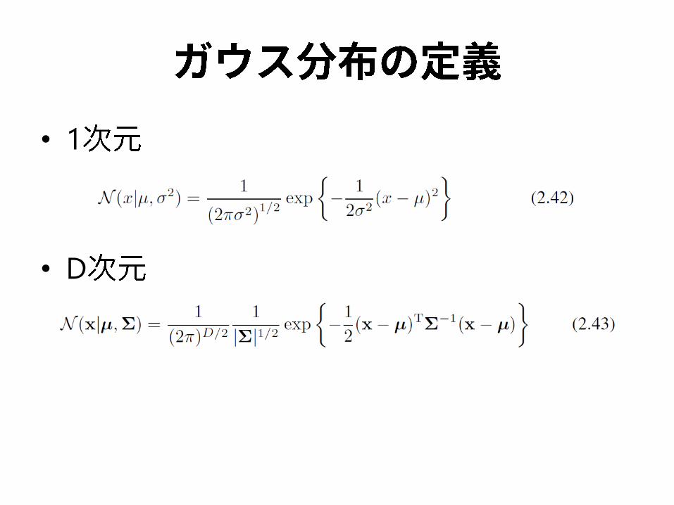
• 1
• D
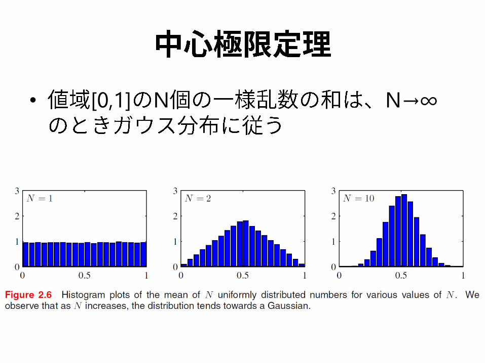
• [0,1] N N→∞
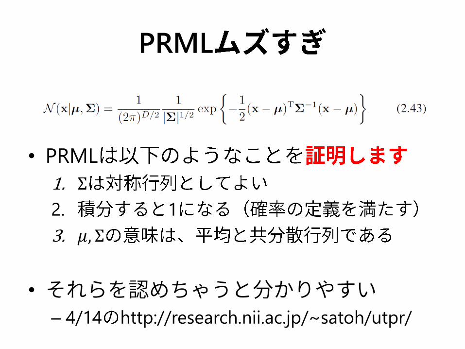
PRML
• PRML
1. Σ
2. 1
3. 𝜇, Σ
•
– 4/14 http://research.nii.ac.jp/~satoh/utpr/
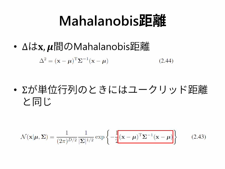
Mahalanobis
• Δ 𝐱, 𝝁 Mahalanobis
• Σ

1. Σ
•
– Exercise 2.17
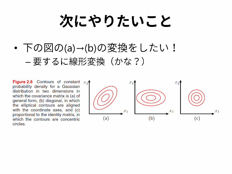
• (a)→(b)
–

(a)→(b)
• Σ
• D …
•
– Exercise 2.18
(a)→(b)
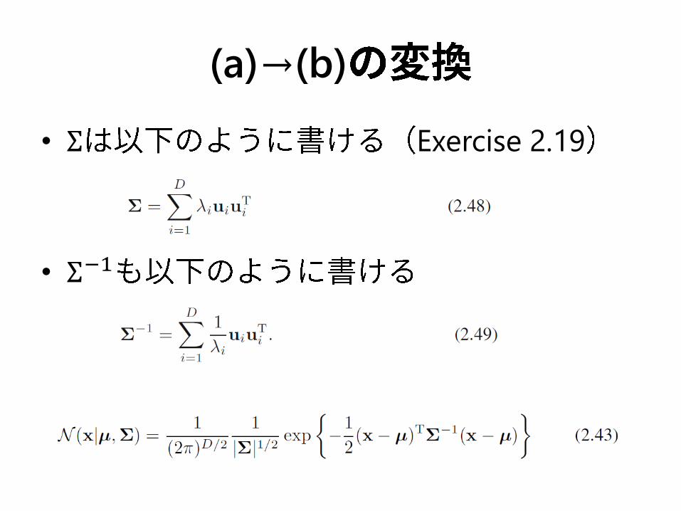
• Σ Exercise 2.19
• Σ−1
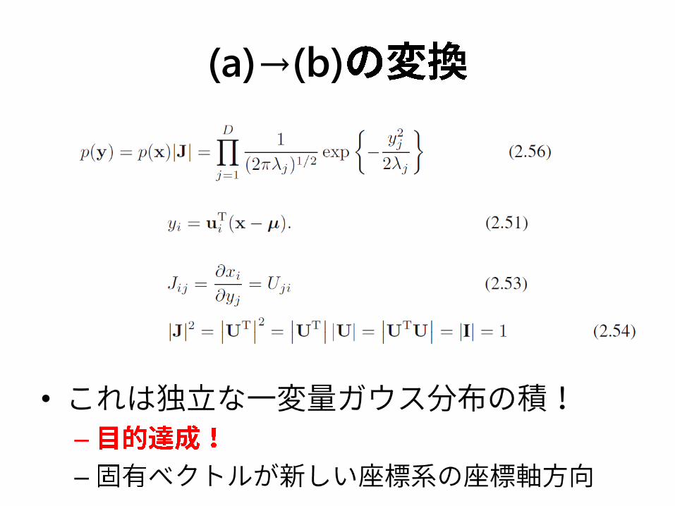
(a)→(b)
•
–
–
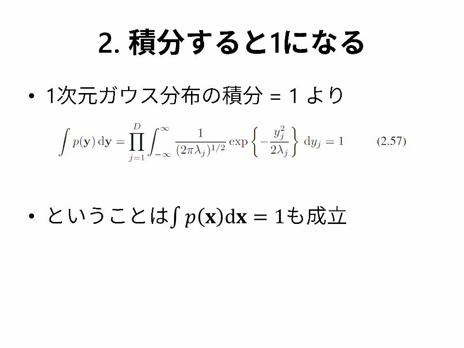
2. 1
• 1 = 1
• 𝑝 𝐱 d𝐱 = 1

3. 𝜇, Σ
0 1
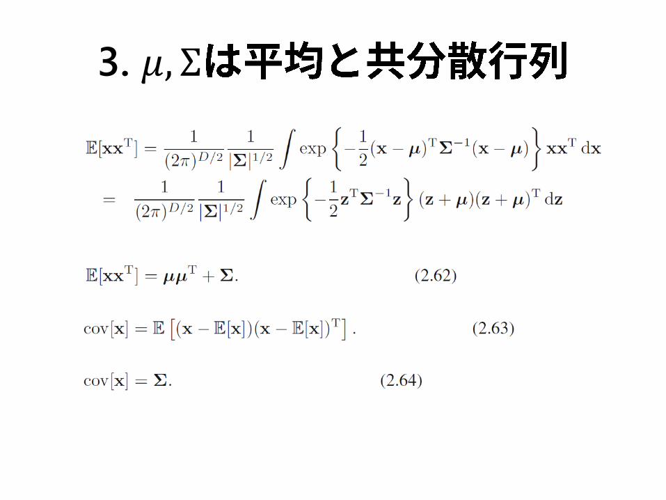
3. 𝜇, Σ
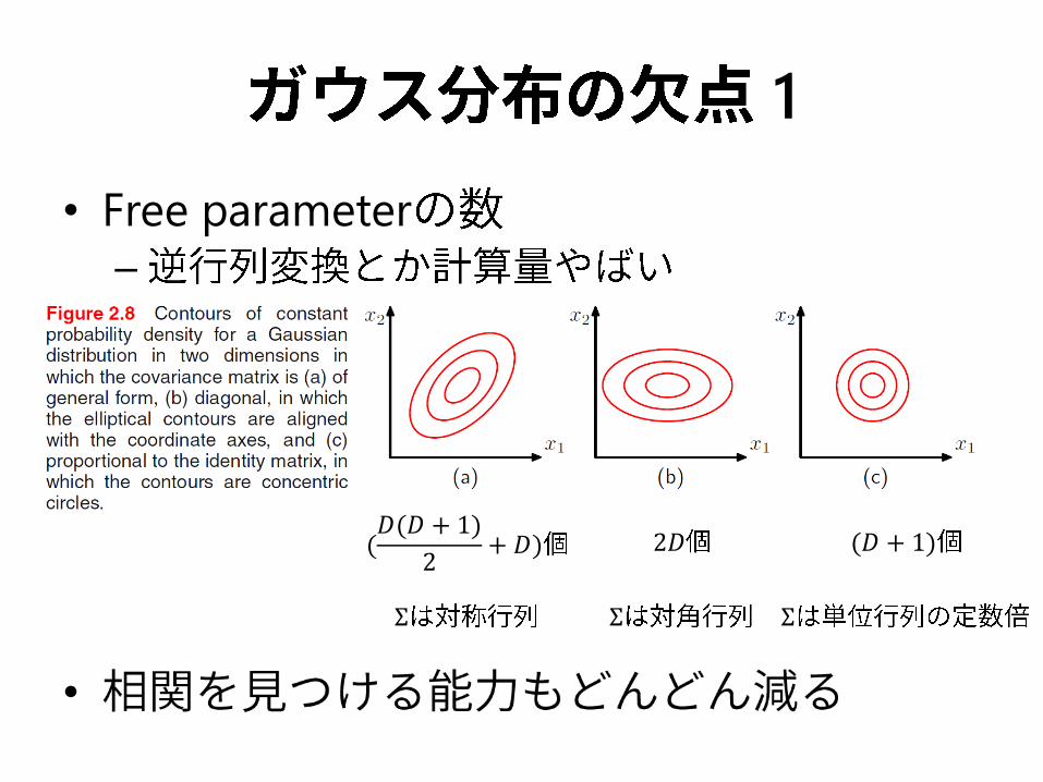
1
• Free parameter
–
•
(𝐷(𝐷 + 1)
2+ 𝐷) 2𝐷 (𝐷 + 1)
Σ Σ Σ
2
• Unimodal i.e.
• Multimodal
• latent variables
1. Section 2.3.9
2. Chapter 12
• Free parameter
• 2 …
– Markov random field Section 8.3
•
– Linear dynamical system Section 13.3
•
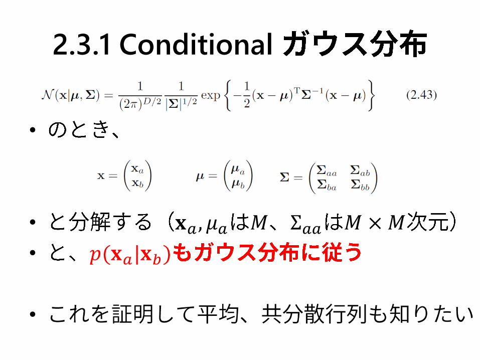
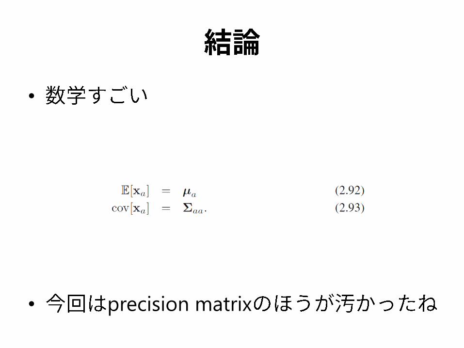
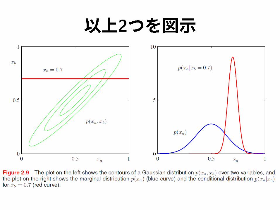
2.3.1 Conditional
•
• 𝐱𝑎 , 𝜇𝑎 𝑀 Σ𝑎𝑎 𝑀 × 𝑀
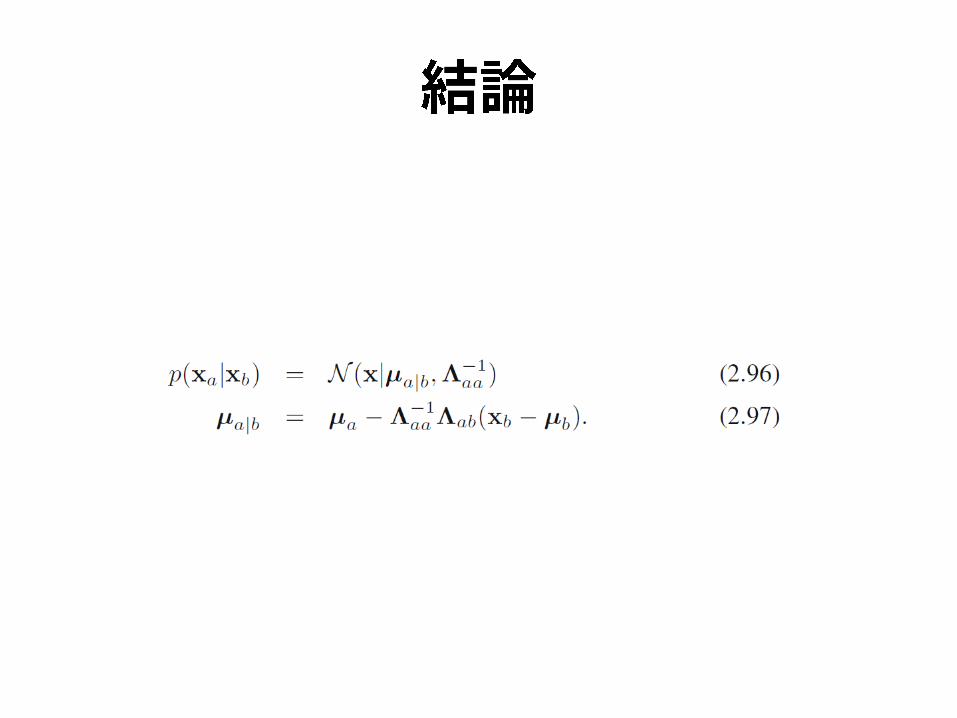
• 𝑝(𝐱𝑎|𝐱𝑏)
•
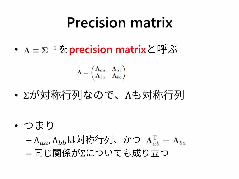
Precision matrix
• precision matrix
• Σ Λ
•
– Λ𝑎𝑎, Λ𝑏𝑏
– Σ
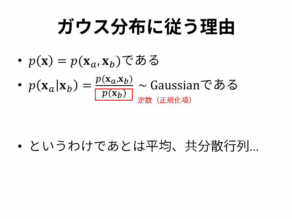
• 𝑝 𝐱 = 𝑝(𝐱𝑎, 𝐱𝑏)
• 𝑝 𝐱𝑎 𝐱𝑏 =𝑝(𝐱𝑎,𝐱𝑏)
𝑝(𝐱𝑏) ~ Gaussian
• …
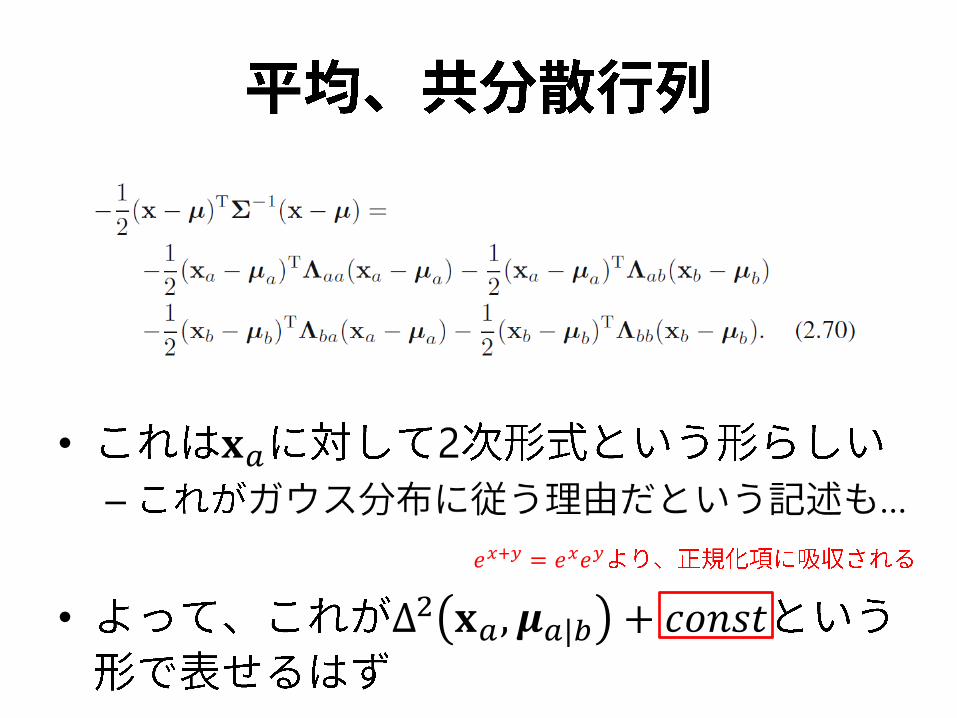
• 𝐱𝑎 2
– …
• Δ2 𝐱𝑎, 𝝁𝑎|𝑏 + 𝑐𝑜𝑛𝑠𝑡
𝑒𝑥+𝑦 = 𝑒𝑥𝑒𝑦
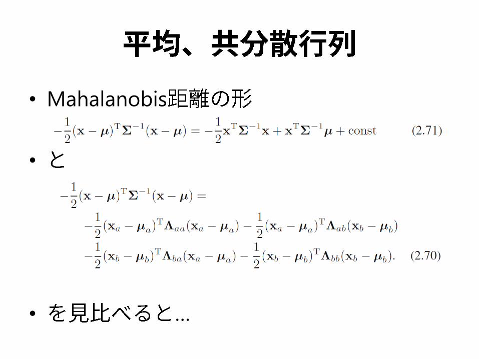
• Mahalanobis
•
• …
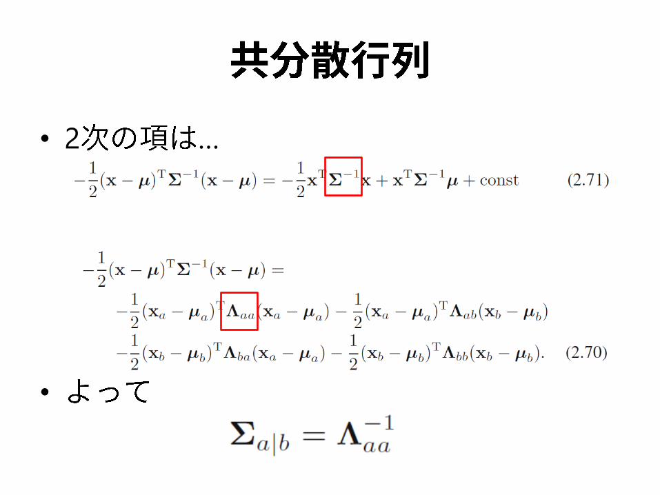
• 2 …
•

• 1 …
• …
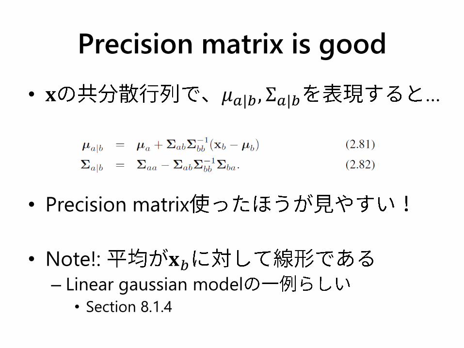
Precision matrix is good
• 𝐱 𝜇𝑎|𝑏, Σ𝑎|𝑏 …
• Precision matrix
• Note!: 𝐱𝑏
– Linear gaussian model
• Section 8.1.4
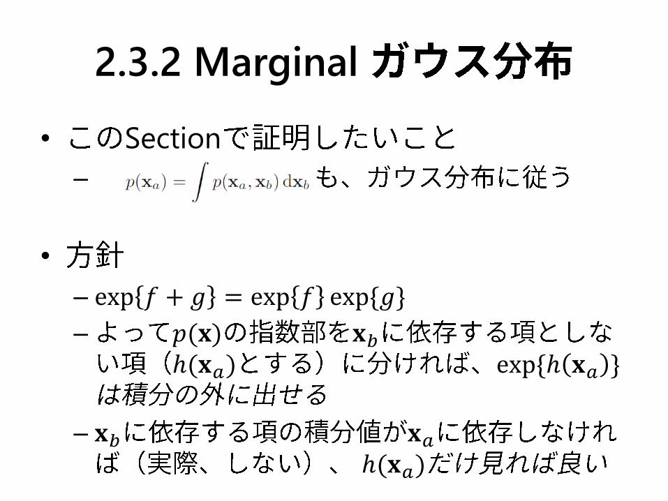
2.3.2 Marginal
• Section
–
•
– exp 𝑓 + 𝑔 = exp 𝑓 exp {𝑔}
– 𝑝(𝐱) 𝐱𝑏
ℎ(𝐱𝑎) exp {ℎ 𝐱𝑎 }
– 𝐱𝑏 𝐱𝑎
ℎ(𝐱𝑎)
𝐱𝑏
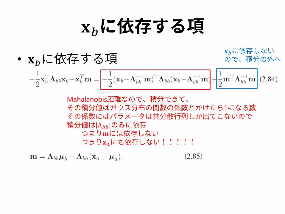
• 𝐱𝑏 𝐱𝑏
Mahalanobis
1
Λ𝑏𝑏
𝐦
𝐱𝑎
𝐱𝑏
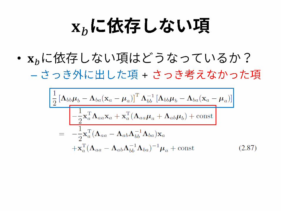
• 𝐱𝑏
– +

• Conditional
•
•

• Conditional
•
• precision matrix
2
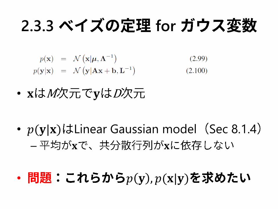
2.3.3 for
• 𝐱 M 𝐲 D
• 𝑝(𝐲|𝐱) Linear Gaussian model Sec 8.1.4
– 𝐱 𝐱
• 𝑝 𝐲 , 𝑝(𝐱|𝐲)
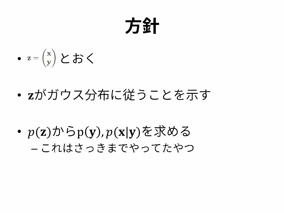
•
• 𝐳
• 𝑝(𝐳) p 𝐲 , 𝑝(𝐱|𝐲)
–
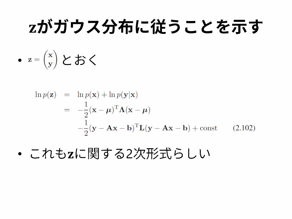
𝐳
•
• 𝐳 2

𝐳
• 2 …

𝐳
• 1 …
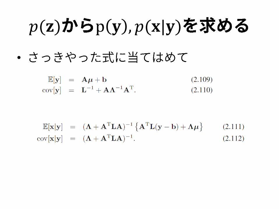
𝑝(𝐳) p 𝐲 , 𝑝(𝐱|𝐲)
•

2.3.4 for
• D N ~𝑁(𝝁, Σ)
• log
• 𝐗 2
sufficient statistics
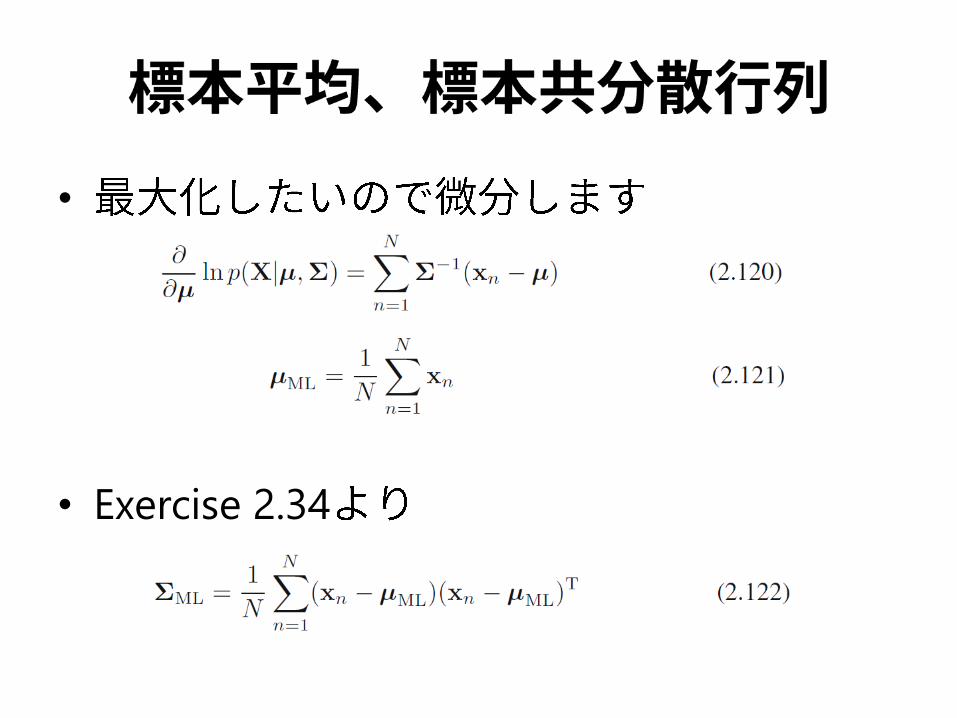
•
• Exercise 2.34
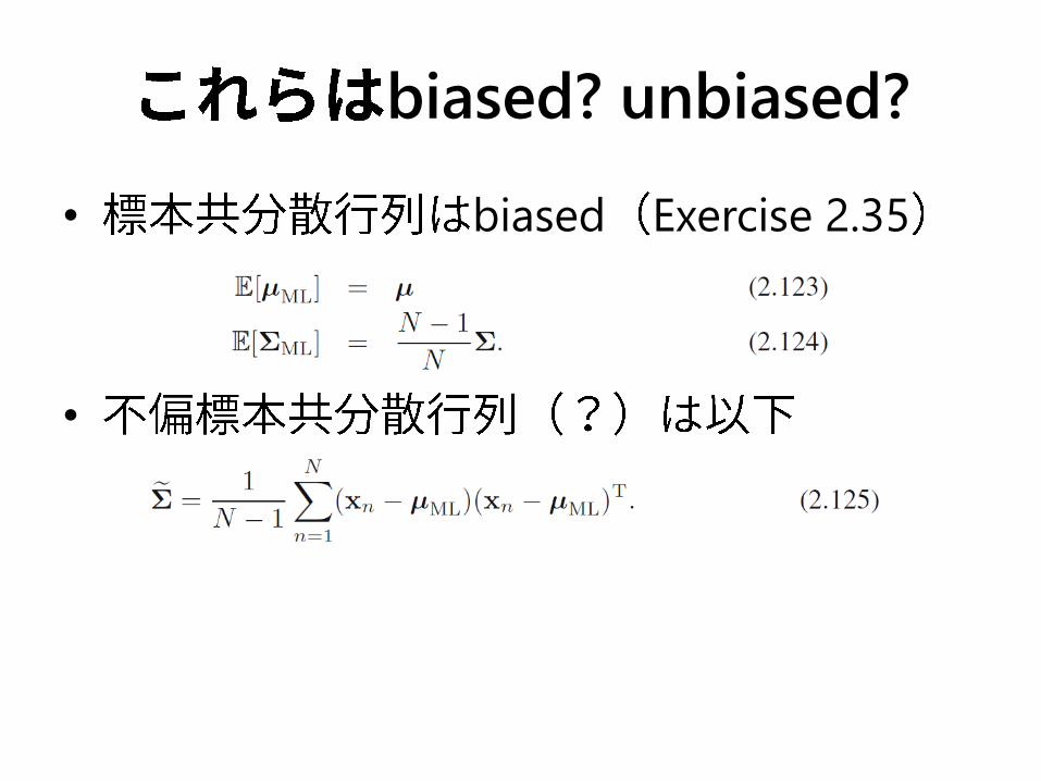
biased? unbiased?
• biased Exercise 2.35
•
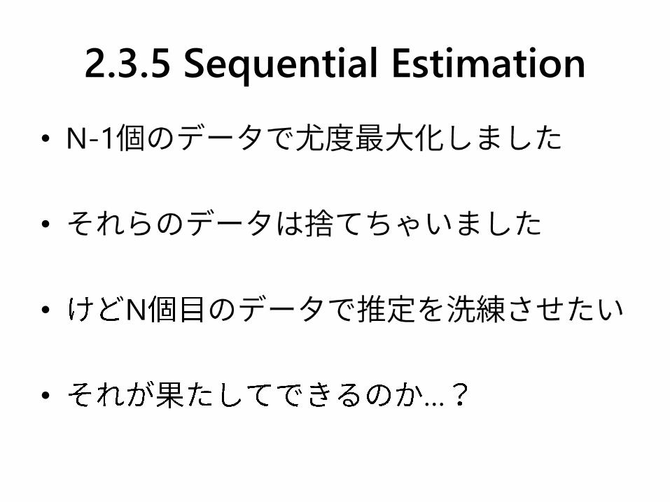
2.3.5 Sequential Estimation
• N-1
•
• N
• …
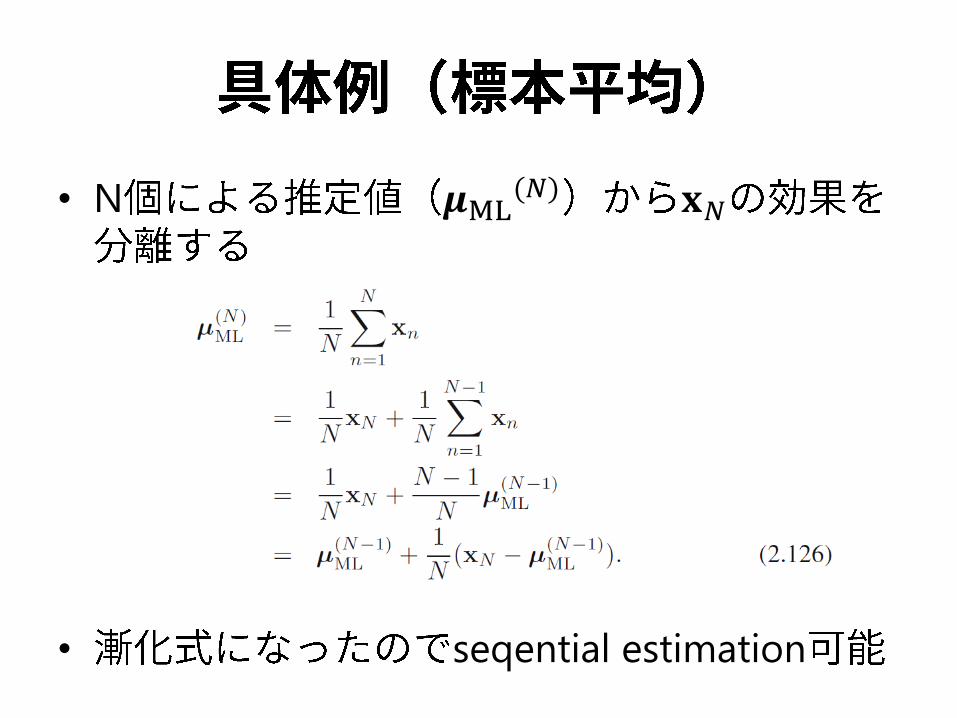
• N 𝝁ML(𝑁) 𝐱𝑁
• seqential estimation
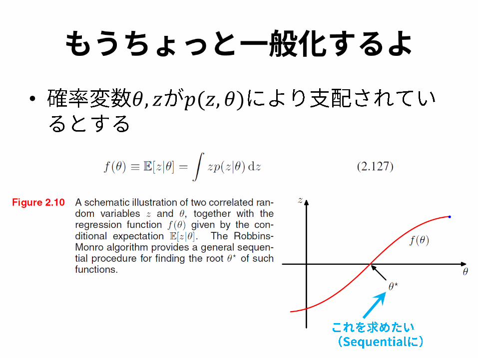
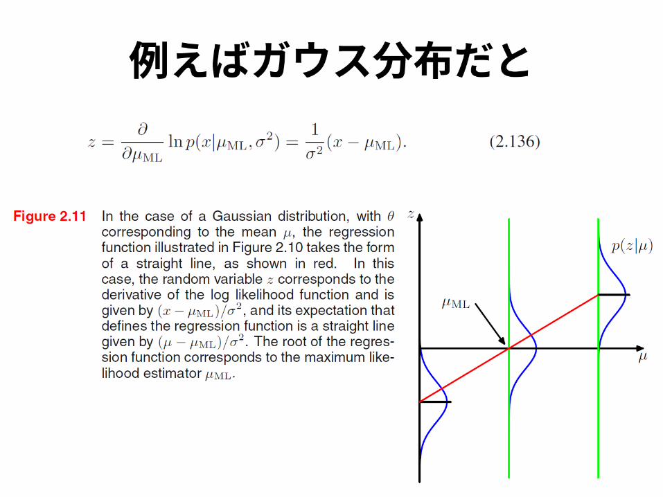
• 𝜃, 𝑧 𝑝(𝑧, 𝜃)

Robbins-Monro
• 1951
•
– z ∞
• 𝑓 𝜃 > 0 ⇒ 𝜃∗ < 𝜃, 𝑓 𝜃 < 0 ⇒ 𝜃 < 𝜃∗
– without loss of generality
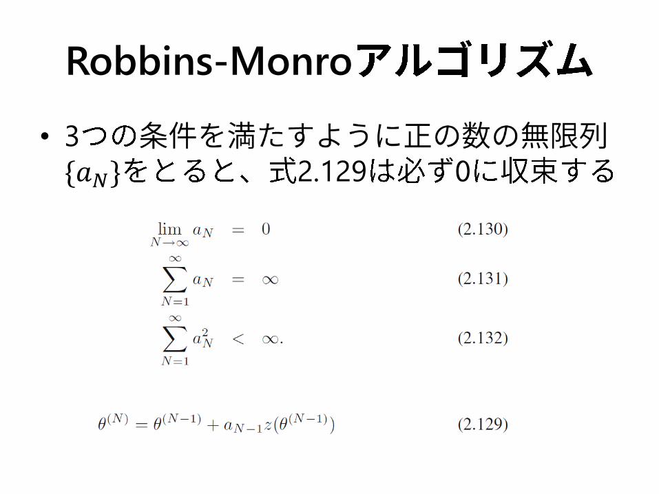
Robbins-Monro
• 3
{𝑎𝑁} 2.129 0


•
[Blum, 1965]

2.3.6 for
•
•
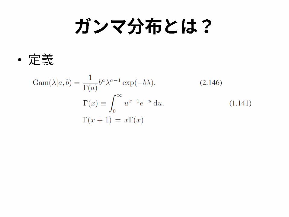
– exp {𝜇 2 }
⇒
⇒
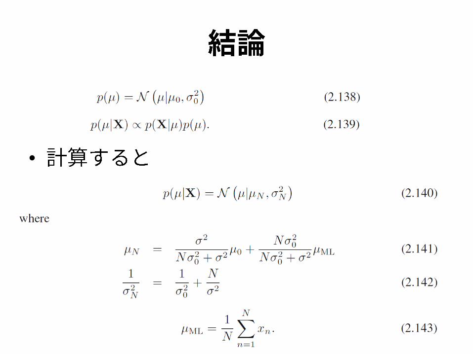
•
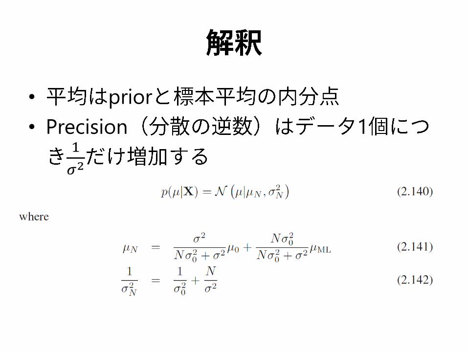
• prior
• Precision 11
𝜎2

•
• D
– Exercise 2.40

Sequential Estimation is easy
•

•
– precision 𝜆 =1
𝜎2
•
– 𝜆𝑛𝑒𝑐𝜆
⇒
⇒
•
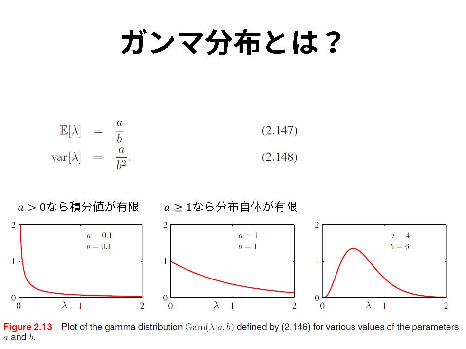
𝑎 > 0 𝑎 ≥ 1
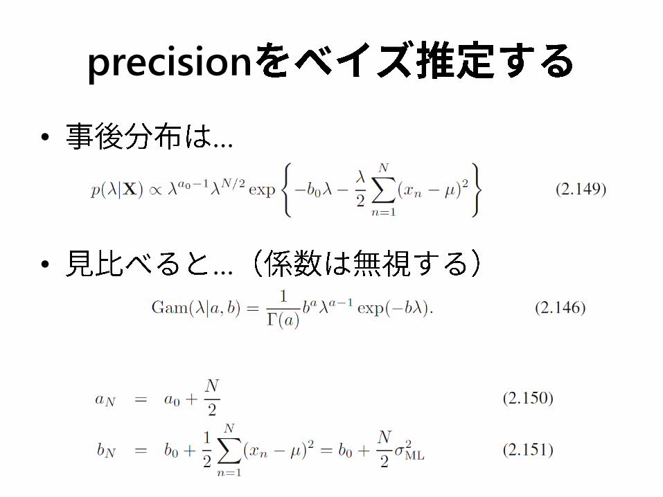
precision
• …
• …

• 𝑎𝑁 N𝑁
2
– 2𝑎0
• 𝑏𝑁 N𝑁
2𝜎ML
2
– =𝑏0
𝑎02𝑎0
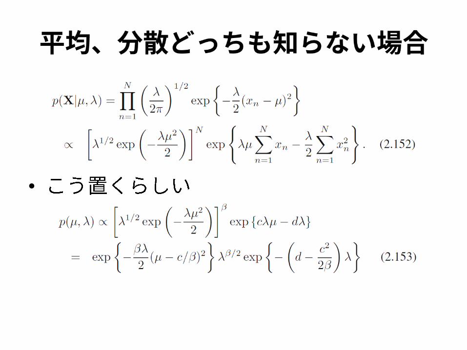
•
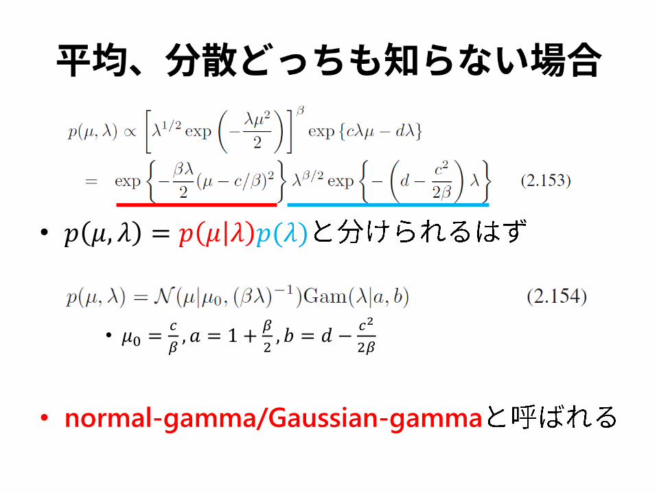
• 𝑝 𝜇, 𝜆 = 𝑝 𝜇 𝜆 𝑝(𝜆)
• 𝜇0 =𝑐
𝛽, 𝑎 = 1 +
𝛽
2, 𝑏 = 𝑑 −
𝑐2
2𝛽
• normal-gamma/Gaussian-gamma
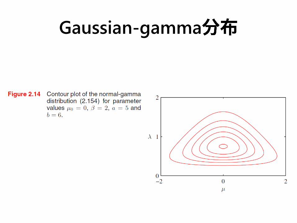
Gaussian-gamma
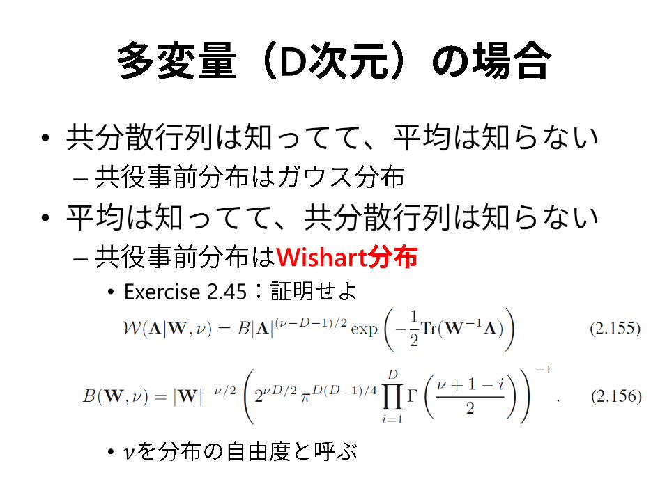
D
•
–
•
– Wishart
• Exercise 2.45
• 𝜈

D
•
– Gaussian-Wishart
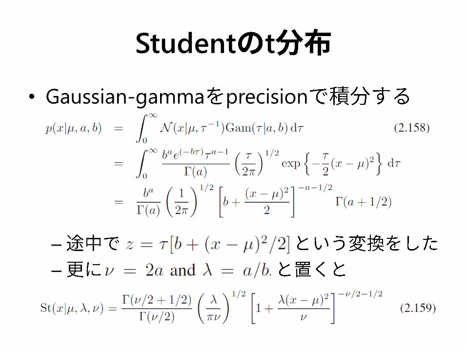
Student t
• Gaussian-gamma precision
–
–
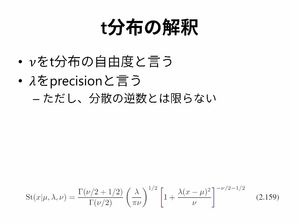
t
• 𝜈 t
• 𝜆 precision
–

t
• 1
• ∞
– Exercise: 2.47:
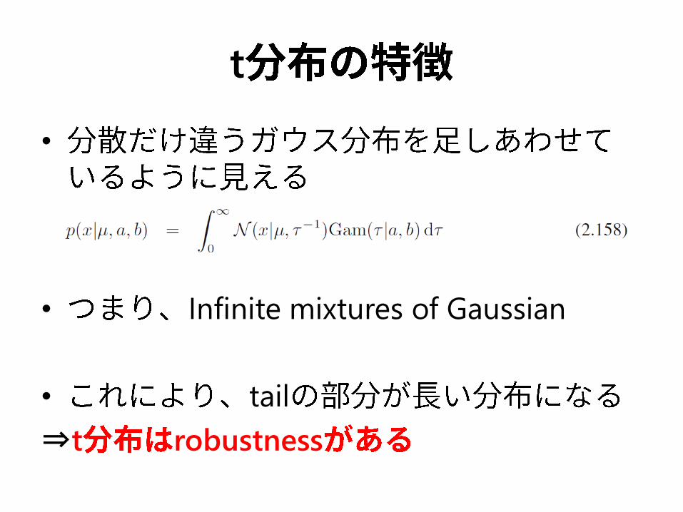
t
•
• Infinite mixtures of Gaussian
• tail
⇒t robustness
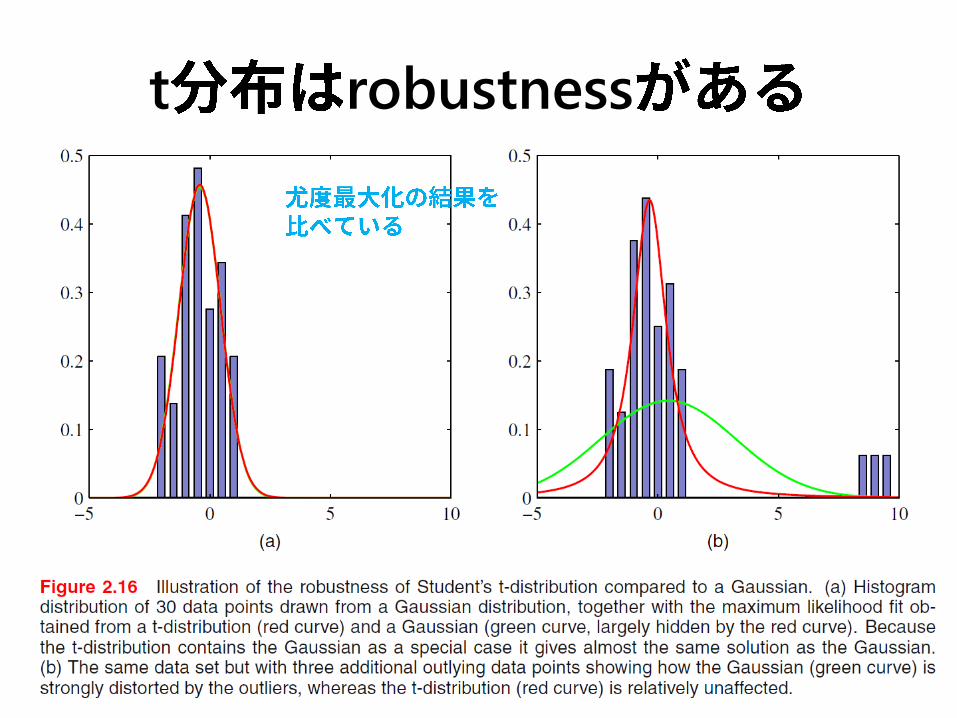
t robustness
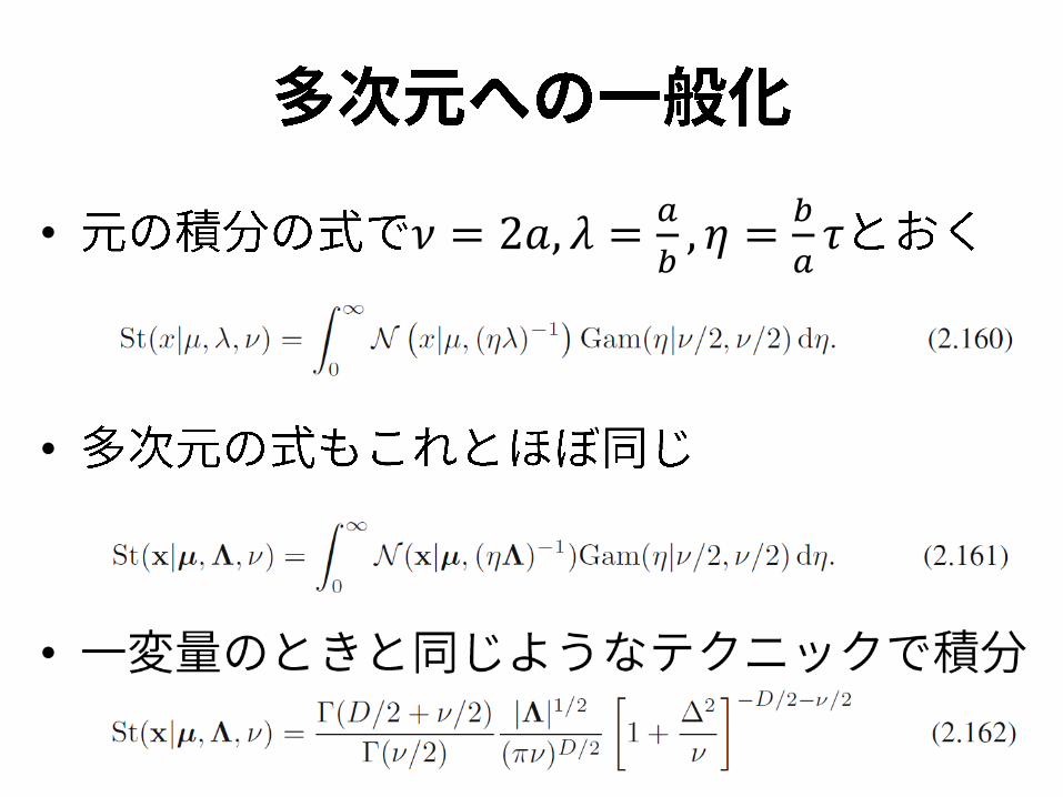
• 𝜈 = 2𝑎, 𝜆 =𝑎
𝑏, 𝜂 =
𝑏
𝑎𝜏
•
•
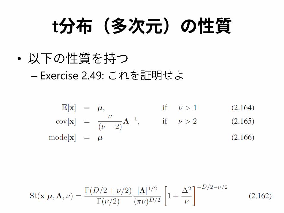
t
•
– Exercise 2.49:

2.3.8
•
– 𝑝 𝑥 = 𝑝 𝑥 + 2𝜋
•
–
•

• PRML
•
Mardia and Jupp (2000)
•
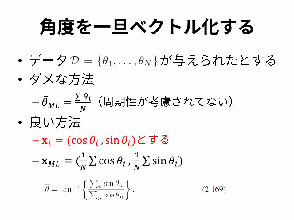
•
– 𝜃 𝑀𝐿 = 𝜃𝑖
𝑁
•
– 𝐱𝑖 = (cos 𝜃𝑖 , sin 𝜃𝑖)
– 𝐱 𝑀𝐿 = (1
𝑁 cos 𝜃𝑖 ,
1
𝑁 sin 𝜃𝑖)
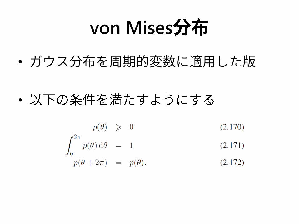
von Mises
•
•
von Mises
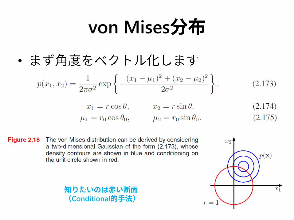
•
Conditional
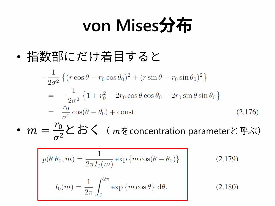
von Mises
•
• 𝑚 =𝑟0
𝜎2 𝑚 concentration parameter

von Mises
• 𝑚
– Exercise 2.52
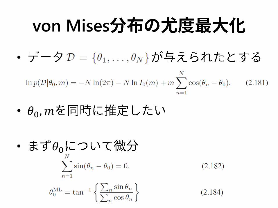
von Mises
•
• 𝜃0, 𝑚
• 𝜃0
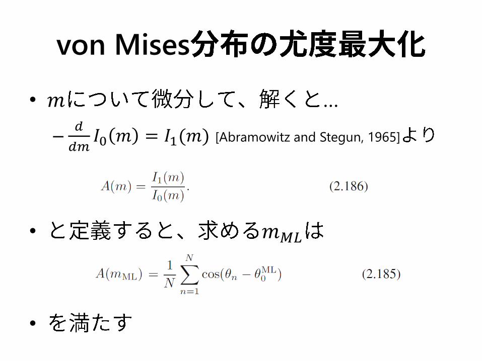
von Mises
• 𝑚 …
–𝑑
𝑑𝑚𝐼0 𝑚 = 𝐼1(𝑚) [Abramowitz and Stegun, 1965]
• 𝑚𝑀𝐿
•
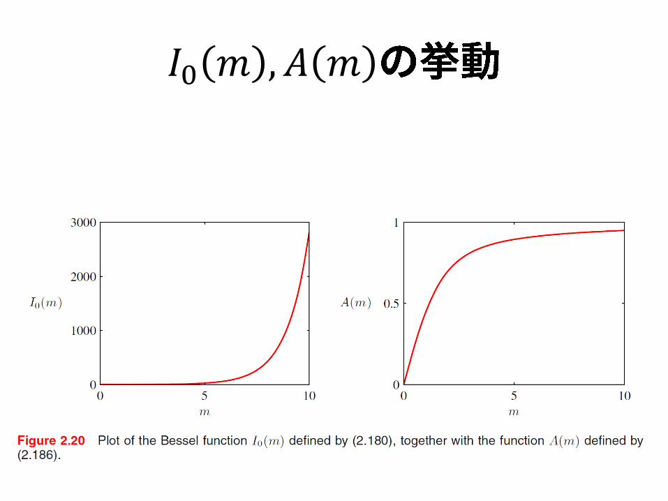
𝐼0 𝑚 ,𝐴 𝑚
•
• Conditional marginal
–
•
• von Mises unimodal
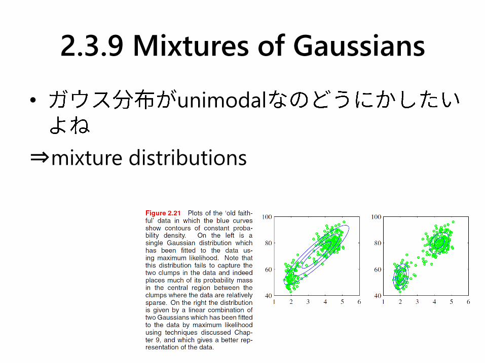
2.3.9 Mixtures of Gaussians
• unimodal
⇒mixture distributions

2.3.9 Mixtures of Gaussians
•
• 1
•
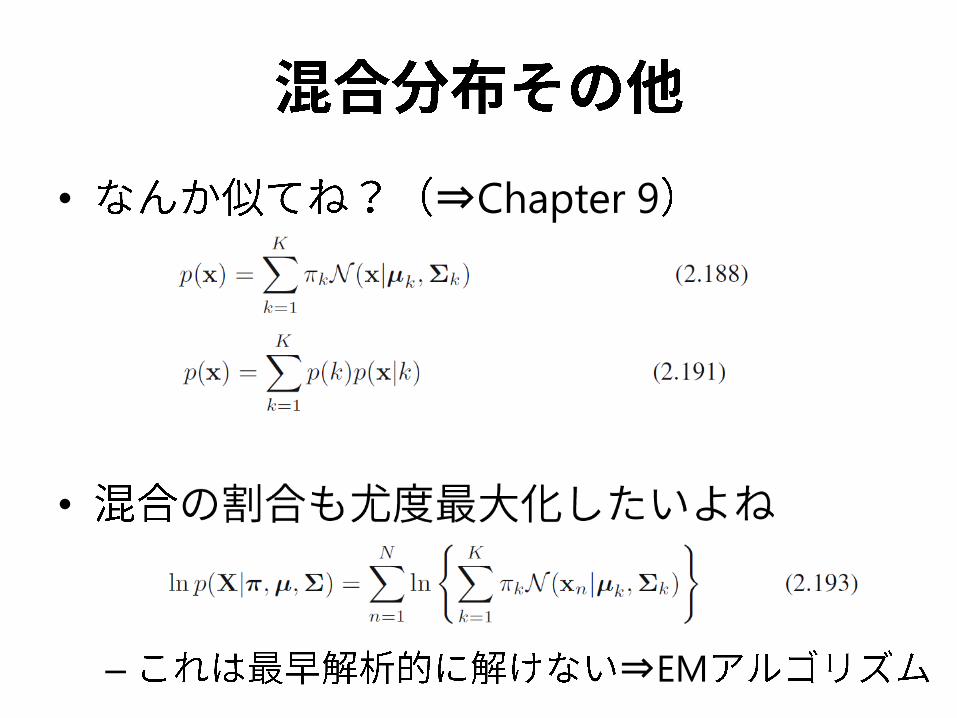
• ⇒Chapter 9
•
– ⇒EM