
Preparation of Papers for Thesis in...
35
석사 학위논문 Master's Thesis 단어를 이용한 트위터 상의 사용자 프로파일 유추에 관한 연구 Inferring user profile using textual content on Twitter 류 경 민 (柳 憬 旻 Ryu, KyoungMin) 웹사이언스공학전공 Division of Web Science Techonology KAIST 2014
Transcript of Preparation of Papers for Thesis in...

석사 학위논문
Master's Thesis
단어를 이용한 트위터 상의 사용자 프로파일
유추에 관한 연구
Inferring user profile using textual content on Twitter
류 경 민 (柳 憬 旻 Ryu, KyoungMin)
웹사이언스공학전공
Division of Web Science Techonology
KAIST
2014

단어를 이용한 트위터 상의 사용자 프로파일
유추에 관한 연구
Inferring user profile using textual content on Twitter

Inferring user profile using textual content on Twit-
ter
Advisor : Professor Moon, Sue Bok
by
Ryu, KyoungMin
Division of Web Science Technology
KAIST
A thesis submitted to the faculty of KAIST in partial fulfillment of the re-quirements for the degree of Master of Science and Engineering in the Division of Web Science Technology. The study was conducted in accordance with Code of Research Ethics1
2014. .
Approved by
Professor Moon, Sue Bok
[Advisor]
1 Declaration of Ethical Conduct in Research: I, as a graduate student of KAIST, hereby declare that I have not committed any acts that may damage the credibility of my research. These include, but are not limited to: falsi-fication, thesis written by someone else, distortion of research findings or plagiarism. I affirm that my thesis contains honest conclusions based on my own careful research under the guidance of my thesis advisor.

단어를 이용한 트위터 상의 사용자 프로파일
유추에 관한 연구
류 경 민
위 논문은 한국과학기술원 석사(박사)학위논문으로
학위논문심사위원회에서 심사 통과하였음.
2014 년 월 일
심사위원장
심사위원
심사위원
문 수 복 (인)
맹 성 현 (인)
차 미 영 (인)

MWST
20124398
류 경 민. Ryu, Kyoung Min. Inferring user profile using textual content on Twitter
. 단어를 이용한 트위터 상의 사용자 프로파일 유추에 관한 연구
. Division of Web Science Technology. 2014. 93 p. Advisor Prof. Moon, Sue Bok.
ABSTRACT
In the past few years online social media have risen as a key venue for communicating with the public
and monitoring public opinions. People talk about movies they watch, restaurants they visit, and views they
enjoy, insinuating their whereabouts. In order to weigh in the public opinions expressed on such social media
as much as traditional poll results or to optimize businesses for specific class of users, the representativeness
of the opinions has to be accounted for. A profile such as age, gender, and location of users is one of the key
factors in the representativeness, but are not available by default in online social networking platform. The
number of users who make their profiles public is relatively small, compared to the huge number of users in
online social networking services and social media platforms. Besides, there are several studies inferring user
profile on various social networking services, but none of them apply their methods on Korean Twitter users.
In this work we propose a new framework to infer a Korean user's main location of activities, age, and gender
in Twitter using their textual contents. Our approach is based on a probabilistic generative model that filters
local words, employs data binning for scalability, and applies a map projection technique for performance in
inferring user’s main location. Also, we use classifier for inferring user’s age and gender and apply feature
selection for filtering relevant features to classes. We evaluate our method with users who have focused GPS-
tagged tweets or with manually annotated users who use profile-relevant words in their description data. For
inferring Korean user’s location, we report that 60% of users are identified within 10km of their locations, a
significant improvement over existing approaches. And for inferring user’s age and gender, we report that
75% and 88% of users are correctly identified.
Keywords: Social Media, profile, data mining
i

Table of Contents
Abstract ································································································ i
Table of Contents ···················································································· iii
List of Tables and Graphs ········································································· vi
List of Diagrams ···················································································· vii
Chapter 1. Introduction
Chapter 2. Related work
2.1 Location ························································································· 2
2.2 Gender ·························································································· 2
2.2 Age ······························································································ 2
Chapter 3. Korean Twitter Dataset
Chapter 4. Method
4.1 Location ························································································· 7
4.1.1 Probabilistic Model ········································································· 7
4.2 Gender and Age ················································································ 8
Chapter 5. Result
5.1 Location ······················································································· 10
5.1.1 Geographic Distribution Inference of Words ·········································· 10
5.1.1 User Location Inference ·································································· 11
5.1.1 Summary of Location Inference Algorithm ············································ 14
5.1.1 Friendship-Based Location Inference ··················································· 18
5.2 Gender and Age ·············································································· 20
Chapter 6. Conclusions
ii

Table of Tables
3.1 Class related words ··········································································· 6
5.1 Top 10 most used words, their α values, latitudes and longitudes ····················· 13
5.2 Words with high α values ··································································· 13
5.3 Word location estimator results ···························································· 13
5.4 Performance of gender and age classifiers ················································ 20
5.5 Words retrieved by feature selection ······················································ 21
iii

Table of Figures
Figure 4.1 Tweet frequency of “story'' and “Busan'' ··········································· 9
Figure 5.1 α versus words ········································································ 14
Figure 5.2 Cumulative distribution of the difference between words' centers and GPS location
from the Google Map ················································································ 14
Figure 5.3 Performance of methods ····························································· 15
Algorithm 1 Find location of users ······························································ 17
Figure 5.4 Performance of inference using friend's words ··································· 19
Figure 5.4 Accuracy per # of words in gender and age classifier ··························· 22
iv

Chapter 1. Introduction
In the past few years online social media have risen as a key venue for communicating with the public
and monitoring public opinions. In order to weigh in the public opinions expressed on such social media as
much as traditional poll results, the representativeness of the opinions has to be accounted for. User profile
is one of the key factors in the representativeness. Yet, most users of online social media do not make their
profile information public. Since Twitter users do not have to enter their profile information on the Twitter
profile, large majority of users do not open their profile to the public. Especially, most of the Twitter users do
not want to provide their location information. Only 34% of Twitter users have meaningful location infor-
mation in their profiles, and less than 1% of Twitter users tag their tweets with GPS locations.
In this work we propose a new approach to infer a Twitter user's gender, age and location. Previous
work has investigated spatial correlation between web resources and user profiles (gender, age and location)
but they have not studied in Korean because of the language characteristics. Inferring user’s gender and age,
we use classifier and implement feature selection to improve performance. Our method estimates over 75%
user’s age and 90% of user’s gender. Inferring user’s location, we use maximum likelihood approach. From
GPS-tagged tweets we extract the spatial correlation between words and GPS locations and refine the city-
level granularity of previous work to 500m distance bins. We use data binning to reduce computational cost.
Also, computing the Euclidian distance from the longitudes and latitudes will cause distortion and we use map
projection to convert between coordinates of longitudes and latitudes and of the 3D Euclidian space. We veri-
fy the accuracy of our approach with large-scale data of Korean Twitter users. Our method estimates 74.9%
of user locations correctly within 10km of their main locations.
The rest of the paper is organized as follows. In Section2 we review related work, and data collection
methodology is in Section 3. Section 4 demonstrates inference methods of location, gender and age. In Sec-
tion 5 we present result of inference. We conclude in Section 9 with a brief discussion for future work.
- 1 -

Chapter 2. Related Work
2.1 Location Geographic locations of users on online social networking services are of paramount importance in
marketing, advertising, and public opinion polling. Yet most users do not specify their towns of residence or
use the GPS tagging feature. From the few users with annotated locations and GPS tagged status updates,
inference techniques mine location information of unknown users [2,3,8,11].
One set of location inference techniques relies on the social network of users. Sadilek et al. examine
the location information and the social network of users with annotated locales and predict the location of
their friends using a dynamic Bayesian network [12]. Jurgens et al. utilize reciprocal relationships on Twitter
and estimate user locations. They report a success ratio of 7% on inferring users' locations on Twitter even
without the textual contents in social media [8]. The authors argue that a user's network in social media is a
pertinent source of information for inferring user location. They also demonstrate that mixing multiple social
media datasets have the potential to improve the accuracy and infer locations on another social network.
Another approach is to take advantage of user-generated contents. Location inference of search en-
gine queries and web pages has produced the idea of power and spread [4,13], and Backstrom et al. refine it to
build a probablistic model for spatial variation [1]. Hecht et al.. produce a descriptive report on Twitter users'
behavior. According to their paper, a low ratio of 34% Twitter users did not enter their actual geographic
information on their profiles. They use a term-frequency-based Multinomial Naive Bayes model on textual
contents and estimate state-level user locations in the US [7]. Cheng et al. propose a probablistic framework
similar to Backstrom's et al. and refine the noisiness in tweet words by a local word classifier. They demon-
strate that by filtering out non-local words, the estimation error is reduced from 1,773 miles to 539 miles.
Also they employ smoothing to address the data sparseness and places ''51% of users within 100 miles of their
actual locations.''
2.2 Gender Inferring gender of Twitter users, most of the researchers use classifier as two classes. Some of the old
sociologic studies classify gender more than two classes, but we can assume that there are only two classes in
Twitter, male and female, biologically.
As other text classification studies have shown, SVM classifier outperforms the other classifiers such
- 2 -
as logistic regression, decision tree, and Naïve Bayes in classifying gender in Twitter [14-19]. Using classifi-
er, the most important factor is controlling features in user vectors. Some studies use specific words that are
decided by authors. Those words are selected because previous socio-linguistic studies say they have power of
discriminating gender. But most of the studies every words or N-gram words as feature [15,17,18]. Rao et al
proposed three models for inferring user gender in Twitter, Socio-linguistic model, Ngram model, and stacked
model [14]. Twitter users use ellipses, emoticons, and other lexical features in their tweets. Socio-linguistic
model uses those lexical features selected by researches in sociolinguistics. The authors compare performance
of those three models and stacked model, which combines socio-linguistic model and Ngram model, shows
best result. Although the result of the Ngram model is better than that of socio-linguistic model, the discrep-
ancy is less than 2%.
Other studies use Ngram words, k-top used words, and emoticons, special letters in users’ tweets.
Bamman says swear words are more related to male, emoticons and special letters are more related to female
[16]. Zamal et al use not only user’s own words but also their friends’ words. The study says that joined clas-
sifiers which combine user’s words and friends’ words shows best result to infer user gender [18].
Name can also be a good feature of inferring gender. Burger et al use user’s first and last name with
tweet and description texts to infer gender. Using name, performance of classifier can be improved more than
10%. Liu et al also use user’s name to infer user gender. They use two different ways. First is using only
names that belong to only one side. Second is setting threshold that distinguish names which have inferring
power [19].
2.3 Age The method of inferring user age in Twitter is similar to inferring user gender in Twitter. Most of the
studies use classifier to infer user age. Features are also similar to the case of inferring user gender. Studies
inferring user age in Twitter use Ngram words, ellipsis, emoticons, and other lexical features [14,18,20]. The
biggest difference between inferring user gender and inferring user age is the number of classes. Inferring
gender, there are only two classes, male and female, but there are various classes in the studies of inferring
age. Rao et al use [30+, 30-] age classes, Zamal et al use [18+, 25+] classes, and Nguyen use [20-, 20-40,40+]
classes [14,18,20]. Since the number of classes affects the performance of classifier, performance of each
study varies in inferring age.
Nguyen et al not only use age classes but also life stage classes. The authors say performance of using
age classes is better than that of life stage [20]. Furthermore, the authors directly infer age using regression,
- 3 -

not divide the classes. Understandably, performance in this case is 20% lower than that of the case using di-
vided classes. The authors also analyze the text of users in classes, and show the number of retweet, link, and
hashtag vary when age classes are changed. The authors say the longer and the more informative the text is,
the older the writer is. Also, younger people talk more about themselves than the elders.
Most of the studies inferring user gender and age in Twitter use English data, especially United States.
But some studies use other countries such as German, Nigeria, and Spain. Though the languages of those
countries are different, discrepancy of classifier performance is less than 5% [17,20].
- 4 -

Chapter 3. Korean Twitter Dataset
We have chosen Korean as the target langauge for this work. Most social media analyses have focused
on English contents, and other languages have received relatively less coverage. As demographics, geogra-
phy, and NLP (Natural Language Processing) tools all differ by the country and the language, we believe this
work is interesting in its own right for designing and evaluating a location inference technique.
In order to find Korean users on Twitter, we used snowball sampling. Starting from two Korean celeb-
rities with more than 100,000 followers, we crawled those celebrities' followers, but limited to those who have
at least one tweet written in Korean among their 200 most recent tweets. Using the Twitter API from June
2010 to April 2011, our crawl resulted in 615 million tweets and 3.3 million Korean user profiles. Our dataset
consists of tweets, user profiles, and following-follower relationships. Twitter provides two types of location
information: the location field in the
user profile and GPS tags of tweets. According to Hecht et al. most users leave the location field blank
or do not write the formal location name [7]. Fewer users turn on the GPS tagging feature on their
smartphones [8]. In our dataset of 614million tweets, only 0.4% or 2.8 million tweets from 140,275 users
have the GPS tags. These users with GPS-tagged tweets form the ground truth in evaluating our tweet-based
location inference.
With the GPS tagging on, a user is associated with multiple locations but a large portion of tweets
come from the user's home or workplace [5]. In order to identify the single location of most representative-
ness to a user, we take the geometric median m, of all the GPS positions calculated as below and label it as the
user's location. It can be the home, workplace, or some other location of frequent visits by the user.
where L is a set of GPS locations of a particular user and distance is the physical distance between the
two points.
In order to filter out those who often have travelled far or who have too few tweets with GPS tags from
the center location, we limit to those who have at least 5 tweets within 15km of their center location as
Jurgens has done in [8]. Also, we sort out 826 social spammers using features as Lee et al. has done in [9].
- 5 -

The final tally is 22,525 users. Of these users' tweets we apply the Korean Morpheme Analyzer KKMA and
extract 801,505 words.
Table 3.1 Class related words
Class Class related words
Gender 남자, 남, 여자, 여, 여자친구, 남자친구, 남친, 여친, 엄마, 아빠, 아줌마
Age 10 대, 85 년생, 04 학번, 30 살, 초, 중, 고, 대학
In order to create the ground truth set of users for inferring user’s age and gender, we first find age or
gender related words to sort out loosely class-related set of users. We count the frequency of words in our
dataset, and manually inspect to find class-related words. Table 1 shows class-related words of each class.
Then we gather users who use at least one class-related word in their description. We found 5145
male-related users, 4191 female related users and 4788 estimated users who are in their 10s, 7588 in 20s, 5134
in 30s and more.
Finally, we manually inspect the users in each class so that we can be sure the user is in the class or
not. We gather 1500 male/female users and 700 10s/20s/30s users.
- 6 -

Chapter 4. Method
4.1 Location
System In this section, we present the basic idea of how we select local words in tweets. We examine
the word's spatial locality in order to determine whether the word can be labeled as local. Words such as
“time'', “story'', or “politics'' do not show clear spatial locality because their use is not limited to a confined
area, but is spread widely. On the other hand, words such as city names, names of local soccer teams, and re-
gional dialects show spatial locality. Figure 1 shows the tweet frequencies of the terms “story'' and “Busan''
in bars of 500x500 m2 grids over the map of Korea. The term “story'' appears with similar frequencies at
many locations, while the term “Busan'' which is the second largest city at a diagonal opposite corner from
Seoul has the peak frequency coinciding with the actual location of the city.
4.1.1 Probabilistic Model Recently, Backstrom et al. have proposed a generative probabilistic model that estimates a search que-
ry's physical location [1]. Their work is based on Yahoo!'s searchquery log. When a user issues a query, the
search engine logs the query along with the user's IP address. If a query is local in nature, the query is likely to
map to a single location near the IP's geolocation. If the query bears no strong relevance to a specific geo-
graphic location, then the query is not easy to be pinned down to a location. Backstrom et al. parameterize the
query's geographic distribution with a focus and a dispersion and estimate them using a maximum likelihood
approach.
Cheng et al. uses Twitter text contents to infer user locations at the city-level granularity [3]. A tweet
is often a sentence or more with multiple words and just as in Backstrom's case not all queries or words have
geographic relevance. Cheng et al. augments Backstrom's approach with classifiers in local word selection
and smoothing.
Below we present a quick sketch of the probabilistic model that underline both approaches. The model
posits that every word has a center, away from which the frequency decays fast. Let Sj and Sj be the set of
tweets that contain the word j (or of queries indexed by j) and its complementary set, respectively. The dis-
tance dij is between the GPS tag of the tweet i and the center of the word j.
Then, the likelihood function f is defined as:
- 7 -

where a constant Cj represents the frequency of the word j at the center, and an exponent value αj de-
termines the dispersion of word j from the center. Backstrom et al. prove that f(C,α) is concave for both C and
α, which guarantees f(C,α) to have exactly one local maximum over its parameter space. A large value of α
determines a quick decay away from the center and thus represents high locality near the center.
4.2 Gender and Age To infer gender and age, we create classifier. First we derive all the Korean words from the tweets in
ground truth user using HAM. Feature set contains these words. We include nouns, verbs, special letters, and
numbers. Though many other studies inferring English user gender and age use Ngram words as features,
HAM already include Ngram-like words in our feature set because some Korean words hard to divide with its
meaning.
We create classifier with those words. We use SVM, Naïve Bayes, decision tree, and logistic regres-
sion. SVM is the most accurate classifier in those four. Decision tree and logistic regression are as good as or
a little bit less accurate and the discrepancy is less than 0.01%. Although SVM is the best, it requires over
twelve hours classifying training set. On the other hand, the running time of logistic regression is less than 10
minute, thus we use logistic regression to classify gender and age.
Next, we use feature selection to refine feature set because some features are more related to classify.
For example, classifying gender, the word “오빠” is used by female mostly. Words like “오빠” have more
part in classifying gender than that of the words like “마을” which is not related to gender. We use mutual
information which is widely used in text classification methods.
Finally, we use words in user description except words such as we used for select ground truth set. The
performance of the classifier is in the next chapter.
Inferring gender, we use name additionally. First we get the member names in boys and girls high
school reunion membership sites because there are only male in boy high school and only female in girl high
school thus we are able to sure that those names are male’s or female’s. We gather 30008 boy names and
15479 girl names. To ensure the name is one gender-sided, we do not use names which are in intersection set
of gender. In the training set, about a half of the users have Korean name in their profile. Before using the
classifier, we infer user gender with those names. We infer user as male if he have male name and female if
she have female name.
- 8 -

(a) story
(b) Busan
Figure 4.1 Two words “story'' and “Busan'' to demonstrate spatial locality of words. The area of the bar
is 500x500m2 and the height represents the tweet frequency.
- 9 -

Chapter 5. Result
5.1 Location
5.1.1 Geographic Distribution Inference of Words At the end of Section 3 we are left with 801,505 words from 22,525 users' tweets for ground-truth
building. First, as the center of a word, we use the center of mass of all the GPS locations of the word's
tweets. Then we use the probabilistic model presented in Section 4.1 and compute the focus and dispersions
of the words. When computing the focus and dispersions, we bin the distance between the GPS coordinates
and the word's center by 500m for computational scalability. In Table 5.1 we list the top 10 most frequently
used words and their α values, latitudes and longitudes. Of the 10 listed words in Table 5.1 only one word,
Gangnam, α greater than 0.1. It refers to a district in Seoul of about 40 km2 with half a million residents.
Yet its geographic locality of use on Twitter is not confined.
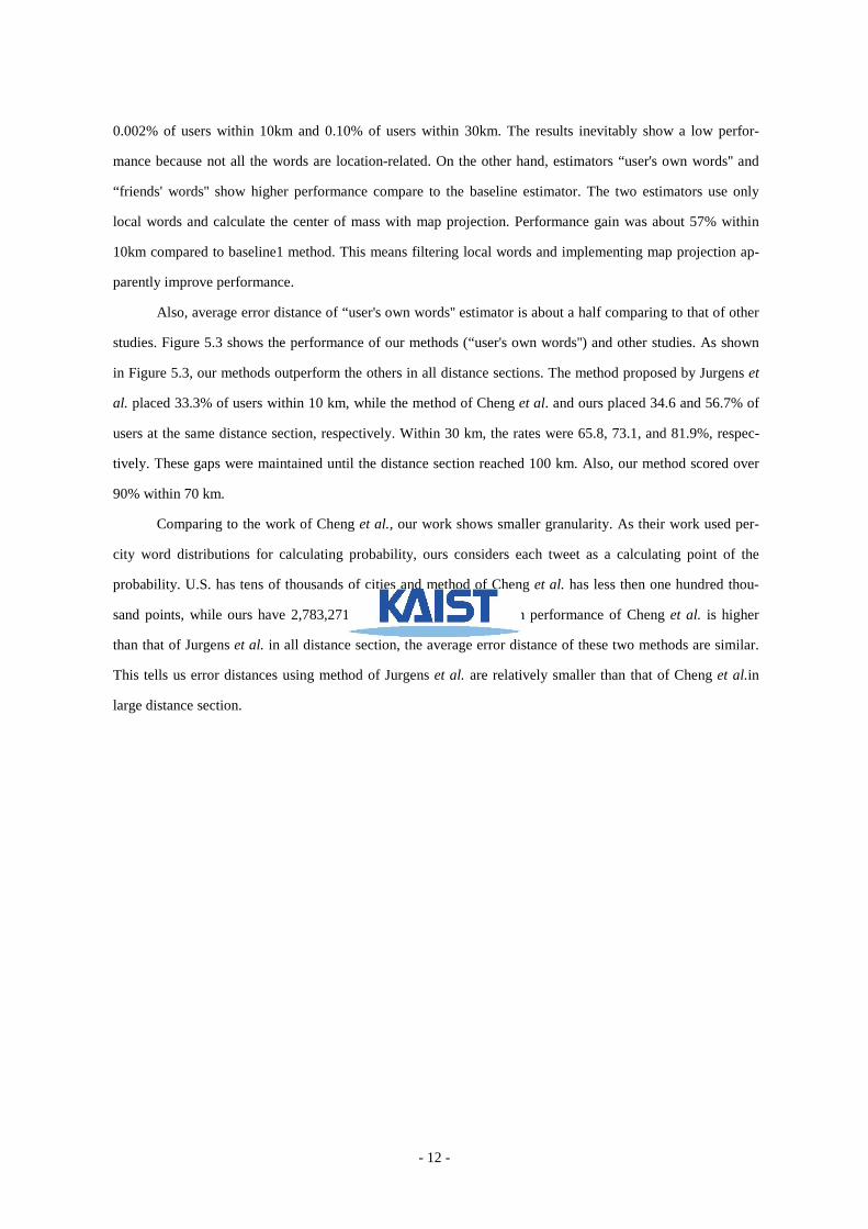
In Figure 5.1 we plot α versus words in decreasing order of α values. About 450 words have α >
0.4. Once α drops below 0.3 beyond 1,000 ranked words, the decline is moderate until the very end.
From the figure we conclude that using the top 1,000 words should provide enough information about spatial
locality of textual contents.
We list the top 10 words with the highest α values and show them in Table 5.2 A quick look gives
us the sense that the words are likely to be very local, as they all refer to cities, station names, and universities,
except for one word “Resource''. The word happens to map to a Korean city by the name of Cheon-an. It
has many companies that deal with scrap metal and recycling and thus the high α is justified. In [1] queries
with a high value of α have shown great locality, while the contribution of C is less pronounced in compari-
son. In [3] they have chosen Bayesian classifiers and identify 3,183 words as local.
In order to evaluate how local they are in our case, we manually inspect the top 1,000 words and pick
712 words easily identifiable to be local. Those words refer to mostly cities, station names, and universities.
For those words, we obtain their GPS coordinates from the Google Map API and compute the difference be-
- 10 -

tween the center from our approach and the Google Map coordinates. Figure 5.2 is the cumulative distribu-
tion of the differences. Among those 712 words, over 70% of the estimated centers fall within 10km of their
actual locations according to the Google Map. As most Korean cities are larger than 20km in width, the ac-
curacy lies at a finer granularity than the city level.
5.1.2 User Location Inference we have used data from all of the 22,525 users in order to evaluate the accuracy of the geographic dis-
tribution inference of words. In this section we use the five-fold approach to build the geographic distribu-
tions of words and evaluate the quality of our user location inference method.
First we begin with the evaluation of our own method, in particular, decisions made at each step.
There are two factors that contribute to the quality of the probabilistic model of local words: the vocabulary
and coordinate transformation. How much accuracy degradation do we see if we use less selective vocabu-
lary of local words? How important is to compute the distance and the center of mass between coordinates
in latitudes and longitudes?
In order to evaluate the importance of local vocabulary, we use the word distributions of all the words
from a user in inferring the user location and call the method Baseline #1. It means we include not only the
top 1,000 words with high α values but all 801,505 words. We state that it is the worst-case scenario for
the case. Next, we use the top 1,000 words for user location inference, but do not employ map project when
computing the user location as the weighted center of mass of words. We label this method Baseline #2.
When computing distance between two pairs of latitudes and longitudes, we use the haversine transformation.
When computing the center of mass among sets of latitudes and longitudes, we have a choice among a
straightforward numerical median (called Manhattan transformation) and the popular Transverse Mercator
transformation, just to name a few. Not including the latter transformation in both baseline methods, we can
evaluate the contribution from the transformation in our method's accuracy.
In order to compare the performance of our method to that of others, we select two studies. we select
studies of Jurgens et al. and Cheng et al. because they are the latest study of a location estimator in Twitter
and the most analogous study to ours, respectively. We apply all of the methods to the same data (Korean
Twitter data that we crawled) and compare our method's performance to that of the others. Table 5.3 shows
average error distance and the performance of word location estimators. “baseline1'' is an estimator calculat-
ing each user's center of mass using all words and not implementing map projection; Also, “baseline2'' is an
estimator using only local words and not implementing map projection. The baseline1 estimator placed only
- 11 -
0.002% of users within 10km and 0.10% of users within 30km. The results inevitably show a low perfor-
mance because not all the words are location-related. On the other hand, estimators “user's own words'' and
“friends' words'' show higher performance compare to the baseline estimator. The two estimators use only
local words and calculate the center of mass with map projection. Performance gain was about 57% within
10km compared to baseline1 method. This means filtering local words and implementing map projection ap-
parently improve performance.
Also, average error distance of “user's own words'' estimator is about a half comparing to that of other
studies. Figure 5.3 shows the performance of our methods (“user's own words'') and other studies. As shown
in Figure 5.3, our methods outperform the others in all distance sections. The method proposed by Jurgens et
al. placed 33.3% of users within 10 km, while the method of Cheng et al. and ours placed 34.6 and 56.7% of
users at the same distance section, respectively. Within 30 km, the rates were 65.8, 73.1, and 81.9%, respec-
tively. These gaps were maintained until the distance section reached 100 km. Also, our method scored over
90% within 70 km.
Comparing to the work of Cheng et al., our work shows smaller granularity. As their work used per-
city word distributions for calculating probability, ours considers each tweet as a calculating point of the
probability. U.S. has tens of thousands of cities and method of Cheng et al. has less then one hundred thou-
sand points, while ours have 2,783,271 points. In addition, although performance of Cheng et al. is higher
than that of Jurgens et al. in all distance section, the average error distance of these two methods are similar.
This tells us error distances using method of Jurgens et al. are relatively smaller than that of Cheng et al.in
large distance section.
- 12 -

Table 5.1 Top 10 most used words, their α values, latitudes and longitudes
Table 5.2 Words with high α values
Table 5.3 word location estimator results
- 13 -
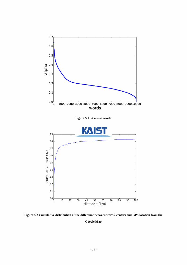
Figure 5.1 αversus words
Figure 5 2 Cumulative distribution of the difference between words' centers and GPS location from the
Google Map
- 14 -

Figure 5.3 Performance of methods. Our method outperforms the others in all distance sections
- 15 -

5.1.3 Summary of Location Inference Algorithm
At the end of Section 3 we are left with 801,505 words from 22,525 users' tweets for ground-truth build-
ing. First, as the center of a word, we use the center of mass of all the GPS locations of the word's tweets.
Then we use the probabilistic model presented in Section 4.1.1 and compute the foci and dispersions of the
words. When computing the focus and dispersions, we bin the distance between the GPS coordinates and the
word's center by 500m for computational scalability.
Then we pick the top 1,000 words with the highest α values. In [1] queries with a high value of α have
shown great locality, while the contribution of C is less pronounced in comparison. In [3] they have chosen
Bayesian classifiers and identify 3,183 words as local.
In order to evaluate how local they are in our case, we manually inspect the top 1000 words and pick
712 words easily identifiable to be local. Those words refer to mostly cities, station names, and universities.
Next, we take the probabilistic generative model from [3] for the spatial variation of queries, and com-
pute the focus and dispersions for each word [3]
for identifying local words. We filter the top 1000 local words among 2,783,271 Korean tweets. Our
method consider all GPS-tagged tweets as a point for calculating probability Cj x di-αj in likelihood function.
We multiply the probability Cj x di-αj to the likelihood function fj if a tweet i have a word j and 1-Cj x di
-αj oth-
erwise. Since millions of GPS-tagged tweets are used to optimize likelihood function, summing all the log
transformed probability up to likelihood function would be computationally expensive. Instead, we put the cal-
culated distances into 500 meter intervals, called bins. In this way, we can reduce computational cost without
losing granularity. Computational cost of our method will be depending on the size of bins. We next calculate
the center of mass for finding the center of each word. All geo-tagged tweets containing a particular word act as
a part of the weight.
To sum up, user location in Twitter is determined as described in Algorithm 1. Line 1~8 describe calcu-
lating the center of each word; line 9\sim16 describe calculating C and α of each word; line 1724 describe cal-
culating the center of each user.
With algorithm 1, we infer location of a user who has at least one local word. However, since not all the
users in Twitter use local words in their tweets, our method cannot be applied to users who do not use any local
words. Thus, we consider another method by taking into account users' friends to alleviate our limitation. We
infer location of users who do not have any local words with their friends' local words (only friends follow the
user back). In this case, the accuracy of the estimator may decrease because the locations of particular user's
friends are not the same as those of the users. Also, Twitter users often follow people who are not physically
nearby. The results are demonstrated in section 5.
- 16 -

- 17 -

5.1.4 Friendship-Based Location Inference In order to infer the location of users who have none of the top 1,000 local words, we resort to their so-
cial network. In this work we define a friend of a user with whom the follow-following relationship recipro-
cally.
Additionally, in order to estimate the location of users who do not have any local words, we apply our
method to them with only their friends' local words (“friends' words in Table 5.3 and Figure 5.4. Inferring loca-
tions with friends' local words also enables acceptable performance, although the performance is lower than that
of inferring with user's own words, as we surmised. In comparison with the method of Jurgens et al., which also
used users' relationship with friends for estimating user location, the performance of the estimator using friends'
local words falls behind only within the range of 15 km to 50 km. However, we note that the method of Jurgens
et al. covers almost all users in the network, while ours only predicts users who use at least one local word in
their tweets including their friends' tweets. Future work will consider a fusion method that reflects the topology
of users on a social network graph to select local words for estimators.
To compare spatial distributions of words in different linguistic culture, we are also interested in investi-
gating language dependency of our method. In addition, the size of a country can significantly influence the
performance of our method since the distortion of map projection depends on the size of the total area. Thus,
future work will consider applying our method to other countries which have different language, culture, and
territory size.
- 18 -

Figure 5.4 Performance of inference using friend's words. This method uses friendship information in
twitter.
- 19 -

5.2 Gender and Age At Figure 5.4 shows performance of classifier when number of features varies. Performances converge
at 3000 for both age and gender. After this step, we proceed with experiment at 3000 features.
Table 5.4 performance of gender and age classifiers
Gender Age
Baseline 0.820 0.679
Using Feature Selection 0.851 0.754
Using Feature Selection + Name 0.878
Table1 shows performance of classifier at each step. Gender classifier shows better performance because
of class number. And since Korean use words which show clear difference between male and female, discrep-
ancy with and without feature selection in inferring gender is smaller than that of age. Words like “오빠”,
“누나” are only used by one side of gender mostly. Also, male and female have different interests. For example,
male users in Twitter talk a lot about politics and they use words like “박근혜”, “대통령”, and “국가”. On the
other hand, female users in Twitter talk about cosmetic, beauty, or soup opera on TV. Also, female users use
lots of smile letters such as “ㅋㅋㅋㅋ” or “ㅎㅎㅎㅎ”. Thus their end of words usually ends with final conso-
nant “ㅋ” or “ㅎ”. They use “했닼ㅋㅋ”, “거얗ㅎㅎ”, or “욬ㅋㅋㅋ”. And female users use a lot of final con-
sonant which show cute shape. They use “얌”,”꺅”,”용”, and “잇”.
Finally, with names, performance of gender classifier is increased once more. Final result of gender
classifier is almost 90%.
- 20 -
Table 5.5 Words retrived by feature selection
남자 여자
형님 군대 인천 언니 티켓 용
위치 직장 아버지 오빠 히 잇
누나 국가 아이 꺅 규 이래
형 미국 페이스 얌 교수님 으
애플 천안 지역 웅 시크 퀴즈
선팔 대한민국 결과 엄마 공연 머리
아내 민국 무료 우왕 치 드라마
대통령 시장 사이트 조아 크림 핸드폰
북한 선 투표 콘서트 짱 수다
앱 담배 교육 크크 완전 궁
10대 20대 30대
오빠 야자 위드당 개강 국민 문재인
비스트 양식 과제 네이트온 박근혜 정부
인피니트 블락비 솔로당 재즈 선거 대선
스티커 아진짜 데스티네이션 에헤헤헤 대통령 기자
뷰티 빅뱅 뮤직어 어려운 대한 대한민국
입금 infinite 설레인당 트친찾기 후보 의원
요섭 가계약 Destination 빠른 뉴스 언론
데뷔 반모 맞팔부탁 학번 국정원 안철수
beauty 자동트윗 멜론뮤직어워드 휴학 민주당 미국
이벵 답멘 벤처 학점 정치 삼성
- 21 -

Figure 5.4 Accuracy per # of words in gender and age classifier
- 22 -

Chapter 6. Conclusions
A large proportion of Twitter users deliberately leave out their location information, incorrectly fill
their location information on the profile, or disable the GPS function on their devices. People tweet about
movies they watch, restaurants they visit, and views they enjoy, insinuating their whereabouts. In this paper
we propose a user location inference method for Korean Twitter users. Previously, Several studies infer Twit-
ter user’s age, gender and location from their textual content. Majority of studies treat English content, espe-
cially U.S Twitter data. User’s culture background, however, can significantly influence the content they cre-
ated.
Inferring user’s gender and age, we use classifier and implement feature selection to improve perfor-
mance. Our method estimates over 75% user’s age and 90% of user’s gender. Inferring user’s location, we use
maximum likelihood approach. From GPS-tagged tweets we extract the spatial correlation between words and
GPS locations and refine the city-level granularity of previous work to 500m distance bins. We use data bin-
ning to reduce computational cost. Also, computing the Euclidian distance from the longitudes and latitudes
will cause distortion and we use map projection to convert between coordinates of longitudes and latitudes
and of the 3D Euclidian space. We verify the accuracy of our approach with large-scale data of Korean Twit-
ter users. Our method estimates 74.9% of user locations correctly within 10km of their main locations.
It remains to develop a hybrid estimator for higher precision of predictions including network-wise in-
formation of the social ties of users. Also, we are interested in applying our method to other countries which
have different language, culture, and territory size from our dataset.
- 23 -

Reference
[1] Backstrom, L., Kleinberg, J., Kumar, R., & Novak, J. (2008),. “Spatial variation in search engine queries”. In Proceedings of the 17th international conference on World Wide Web, pp. 357-366.
[2] Backstrom, L., Sun, E., & Marlow, C. (2010). “Find me if you can: improving geographical pre-diction with social and spatial proximity”. InProceedings of the 19th international conference on World wide web, pp. 61-70. [3] Cheng, Z., Caverlee, J., & Lee, K. (2010). “You are where you tweet: a content-based approach to geo-locating twitter users”. In Proceedings of the 19th ACM international conference on Information and knowledge management, pp. 759-768. [4] Ding, J., Gravano, L., & Shivakumar, N. (2000). “Computing geographical scopes of web re-sources”. 23 pages. [5] Frank, M. R., Mitchell, L., Dodds, P. S., & Danforth, C. M. (2013). “Happiness and the patterns of life: a study of geolocated tweets”. Scientific reports, 3. [6] S. goo Lee. (2010). “KKMA : A Tool for Utilizing Sejong Corpus Based on Relational Data-base”. Journal of KIISE : Computing Practices and Letters,16(11), pp. 1046-1050. [7] B. Hecht, L. Hong, B. Suh, and E. H. Chi. (2011). “Tweets from Justin Bieber's Heart: The Dy-namics of the Location Field in User Profiles”. In Proceedings of the SIGCHI Conference on Human Factors in Computing Systems, pp. 237-246. [8] D. Jurgens. (2013). “That's What Friends Are for: Inferring Location in Online Social Media plat-forms Based on Social Relationships”. In Seventh International AAAI Conference on Weblogs and Social Media, [9] K. Lee, J. Caverlee, and S. Webb. “Uncovering Social Spammers: Social Honeypots+ Machine Learning”. (2010) In Proceedings of the 33rd international ACM SIGIR conference on Research and development in information retrieval, pages 435-442. [10] A. K. F. Melanie A. Rapino. (2013). “Mega Commuters in the U.S.” In Association for Public Policy Analysis and Management Conference, [11] T. Pontes, M. Vasconcelos, J. Almeida, P. Kumaraguru, and V. Almeida. (2012) “We Know Where You Live: Privacy Characterization of Foursquare Behavior”. In Proceedings of the 2012 ACM Conference on Ubiquitous Computing, pp. 898-905. [12] A. Sadilek, H. Kautz, and J. P. Bigham. (2012) “Finding Your Friends and Following Them to Where You Are.” In Proceedings of the Fifth ACM International Conference on Web Search and Da-ta Mining, pp. 723-732.
- 24 -
[13] L. Wang, C. Wang, X. Xie, J. Forman, Y. Lu, W.-Y. Ma, and Y. Li. (2005) “Detecting Domi-nant Locations from Search Queries.” In Proceedings of the 28th Annual International ACM SIGIR Conference on Research and Development in Information Retrieval, pp. 424-431. [14] Rao, D., Yarowsky, D., Shreevats, A., & Gupta, M. (2010). “Classifying latent user attributes in twitter”. In Proceedings of the 2nd international workshop on Search and mining user-generated contents, pp. 37-44. [15] Burger, J. D., Henderson, J., Kim, G., & Zarrella, G. (2011). “Discriminating gender on Twit-ter”. In Proceedings of the Conference on Empirical Methods in Natural Language Processing, pp. 1301-1309. [16] Bamman, D., Eisenstein, J., & Schnoebelen, T. (2012). “Gender in Twitter: styles, stances, and social networks”. arXiv preprint arXiv:1210.4567. [17] Fink, C., Kopecky, J., & Morawski, M. (2012). “Inferring Gender from the Content of Tweets: A Region Specific Example”. In ICWSM. [18] Al Zamal, F., Liu, W., & Ruths, D. (2012).. “Homophily and Latent Attribute Inference: Infer-ring Latent Attributes of Twitter Users from Neighbors”. In ICWSM. [19] Liu, W., & Ruths, D. (2013). “What’s in a name? Using first names as features for gender infer-ence in Twitter”. In Analyzing Microtext: 2013 AAAI Spring Symposium. [20] Nguyen, D., Gravel, R., Trieschnigg, D., & Meder, T. (2013). “How Old Do You Think I Am?: A Study of Language and Age in Twitter”. In Proceedings of the Seventh International AAAI Confer-ence on Weblogs and Social Media.
- 25 -

요 약 문
단어를 이용한 트위터 상의 사용자 프로파일 유추에 관한 연구
최근들어 온라인 소셜미디어가 대중과 소통하거나 여론 파악의 중요한 수단중의 하나가
되어가고 있다. 사람들은 본인들의 관심사, 좋아하는 장소, 또는 사회 문제에 관한 의견 등을
소셜미디어 내에서 서로 이야기하고 소통한다. 하지만 이러한 소셜 미디어 내의 관심이나
의견들이 현실과 반드시 일치하는 것은 아니다. 소셜 미디어가 아직 젊은 나이층을 중심으로
움직이고 있고, 소셜미디어 내의 전체 성별 분포가 어떻게 되는지에 관한 연구가 부족한
상태에서 소셜미디어의 의견이 곧 현실의 의견과 같다고 생각하는 것은 무리가 있다. 따라서
소셜미디어 내의 사용자의 성별이나 나이, 지역 등의 프로필 분포를 파악하는 것은 소셜미디어
상의 의견을 현실에 투영하기 위해 반드시 필요한 과정이라고 할 수 있다. 하지만 많은 소셜
미디어들이 사용자의 프로필을 공개하지 않거나 부분만 공개하고 있고, 의무적인 사항이
아니기 때문에 많은 사용자들이 자신의 프로필을 공개하지 않는다. 또한 보안에 대한 사회적인
우려 때문에 더 많은 사용자들이 자신의 프로필을 공개하는 것을 꺼려하고 있다. 본
연구에서는 이러한 소셜미디어의 사용자 프로필 정보 부족 문제를 줄여보고자 트위터에서
사용자가 올린 단어들을 통해 사용자의 나이, 성별, 위치를 추정하는 방법을 제시하였다.
위치를 유추할 때는 확률 모델을 통해 최대우도추정법(MLE)을 사용하여 단어의 위치
집중도와 확산분포를 파악하여 한곳에 집중되어 있는 단어와 단어의 중심 위치를 우선
찾아내어 위치 관련 단어라고 가정하였다. 그 후에 각각의 사용자가 사용한 단어들 중에 위치
관련 단어들의 중심 위치의 무게중심을 구하여 이를 사용자의 위치라고 추정하였다.
무게중심을 구할때는 지도 투영법을 사용하여 곡면으로 구성되어 있는 지구를 직선으로
가정함에서 오는 오차를 줄여 위치 추정 정확도를 높였다.
성별과 나이를 유추할 때는 사용자들의 단어를 특징(feature)으로 하여
분류기(classifier)를 만들었다. 또한 정확도를 높이기 위해서 특징 선택 방법 중의 하나인 mu-
tual information 을 사용하여 클래스와 관련된 특징을 골라내었다. 성별을 유추할 때는 남,여
고등학교에서 모은 이름 정보를 통해 정확도를 높이는 단계를 추가하였다.
위치 추정 방법을 적용한 결과 10km 이내에서 이전 논문들보다 20%이상 높은 정확도를
보여주었고, 성별과 나이는 이전 논문과 비슷하거나 3% 내외의 조금 나은 정확도가 나왔다.
또한 성별과 나이를 구분하는 단어들을 살펴본 결과 사회언어학에서 나온 성별 및 나이의
특징을 반영함을 알 수 있었다. 이를 통해 우리가 소셜미디어에서 사용하는 언어가 현실에서의
성별 및 나이에 따른 언어 행태를 반영한다는 사실을 유추해 볼 수 있다.
핵심어: 소셜 미디어, 프로필, 데이터 마이닝
- 26 -

- 27 -


![8 1 4 Park, Hosung) - KAISTan.kaist.ac.kr/~sbmoon/paper/thesis/2010Dec-hosung.pdf · 2018-08-30 · A thesis submitted to the faculty of KAIST in partial ful llment ... 22, 13]. Independent](https://static.fdocument.pub/doc/165x107/5f3cce50f3e41a6f75563b79/8-1-4-park-hosung-sbmoonpaperthesis2010dec-hosungpdf-2018-08-30-a-thesis.jpg)