Polarized proof-nets and λμ-calculus

Theoretical Computer Science 290 (2003) 161–188www.elsevier.com/locate/tcs

Polarized proof-nets and ��-calculus

Olivier LaurentInstitut de Math�ematiques de Luminy, 163 Avenue de Luminy - case 907,

F-13288 Marseille Cedex 09 France

Received January 2000; received in revised form May 2001; accepted May 2001Communicated by P.L. Curien

Abstract

We .rst de.ne polarized proof-nets, an extension of MELL proof-nets for the polarized frag-ment of linear logic; the main di3erence with usual proof-nets is that we allow structural ruleson any negative formula. The essential properties (con4uence, strong normalization in the typedcase) of polarized proof-nets are proved using a reduction preserving translation into usualproof-nets.We then give a reduction preserving encoding of Parigot’s ��-terms for classical logic as

polarized proof-nets. It is based on the intuitionistic translation: A → B !A ( B, so that itis a straightforward extension of the usual translation of �-calculus into proof-nets. We give areverse encoding which sequentializes any polarized proof-net as a ��-term.In the last part of the paper, we extend the �-equivalence for �-calculus to ��-calculus.

Interestingly, this new �-equivalence relation identi.es normal ��-terms. We eventually showthat two terms are equivalent i3 they are translated as the same polarized proof-net; thus theset of polarized proof-nets represents the quotient of ��-calculus by �-equivalence. c© 2002Elsevier Science B.V. All rights reserved.

0. Introduction

In the last ten years, much work has been done to solve the so-called determiniza-tion problem for classical logic: .nding some computational interpretation of classicalproofs, similar to the Curry–Howard correspondence for intuitionistic logic. We willbe interested in two kinds of solutions that have been proposed.

• The sequent calculus approach has two main instances: Girard’s LC [5] is a de-terministic sequent calculus for classical logic based on a polarization of formulas,

E-mail address: [email protected] (O. Laurent).

0304-3975/02/$ - see front matter c© 2002 Elsevier Science B.V. All rights reserved.PII: S0304 -3975(01)00297 -3

162 O. Laurent / Theoretical Computer Science 290 (2003) 161–188

with a semantics of proofs in coherent spaces; the LKtq system of Danos–Joinet–Schellinx [3] gives an extensive description of the deterministic reduction strategiesthat may be applied to LK. Both LC and LKtq have translations into linear logicthat preserve reductions (see also Quatrini–Tortora [11]).

• The �-calculus approach consists in extending the �-calculus with control operatorstyped by classical schemes. For example, one adds a new constant call=cc typed bythe Peirce law ((A→B)→A)→A. Unfortunately, the reduction rules for this newconstant depend on the reduction strategy (call-by-name or call-by-value), contra-dicting the Church–Rosser property for �-calculus.The ��-calculus of Parigot [9] on the other hand is based on a natural deductionwith multiple conclusions and enjoys con4uence. As before there are some goodtranslations of ��-calculus into linear logic. Furthermore, it has been recently givena nice categorical semantics, the control categories of Selinger [14], which as aby-product, extends the language of types with a new disjunctive connective.

As in the �-calculus where the �-equivalence [12, 13] identi.es terms that di3eronly in their sequential structure (e.g. (�x1:�x2:u)v1v2 and (�x2:�x1:u)v2v1), ��-calculusterms contain pieces of information, which are unnecessary from the operational view-point. Indeed the control category semantics identi.es distinct normal ��-terms. Sotwo questions naturally arise: 4nd the �-equivalence for ��-calculus; 4nd some paral-lel syntax which identi4es �-equivalent terms. In the �-calculus, these two questionsare answered by means of a translation of intuitionistic logic into proof-nets. However,as to the present work, the translations of ��-calculus into linear logic fail to solvethese problems, essentially because they preserve the sequential information by trans-lating it as exponential boxes (typically the t-translation in [3] de.nes the encoding ofthe classical arrow by: A→B !?A( ?B).In this paper, we set up and study a translation of ��-calculus into polarized proof-

nets (PPN) for the fragment LLP of linear logic [7, 8]. LLP is a subsystem of LLdealing with polarized formulas where polarities are de.ned as a linear version of LC’spolarities. Polarized proof-nets allow a .ner use of exponential boxes: structural rules,which are reserved to formulas of the shape ?A in LL, are now applied to any negativeformula (saving uses of the ? connective). Dually the cut elimination takes advantageof the geometrical properties of polarized proof-nets for duplicating any ⊗-tree (savinguses of the !-boxes). We prove the basic properties of PPN (con4uence, normalization)by using a reduction preserving translation of polarized proof-nets into usual proof-nets which may be seen as an analogue of CPS-translations from ��-calculus into �-calculus.We shall show that the translation of ��-calculus preserves reductions and that it

is surjective. Interestingly enough, it translates A→B as !A(B just like the usualencoding of intuitionistic logic. 1 As a consequence the translation is a straightforward

1 In fact the t-translation may be factorized through ours: .rst use the LLP-translation, then use thetranslation of LLP into LL shown in Section 1.4.

O. Laurent / Theoretical Computer Science 290 (2003) 161–188 163

extension of the �-calculus translation [1, 12]. Furthermore, since there is very little dif-ference between LLP and LC (the two systems are equivalent in the categorical sense),our framework conciliates LC and the ��-calculus, allowing the use of LC as a typingsystem for ��-terms and endowing ��-calculus with LC structure (e.g., its denota-tional semantics). In other terms we have established a Curry–Howard correspondencebetween LC and ��-calculus.We shall also de.ne the �-equivalence for ��-calculus as an extension of the

�-equivalence for �-calculus. We show that it is operationally innocuous as it is in-cluded in the � -equivalence of ��-calculus. This result is slightly weaker than inthe �-calculus since it must make use of -equivalence (whereas �-equivalence for�-terms is included in �-equivalence). We show that �-equivalence is complete w.r.t.the translation: two terms are equivalent i3 they are translated as the same proof-net.For the sake of simplicity, we shall stick to simply typed ��-calculus. However, our

translation is easily extendable to some richer language: pairing may be encoded by the& connective, Selinger’s disjunctive connective may be encoded by the o connective.As in the �-calculus, we can use linear .rst and second order quanti.ers to encodethe classical ones. The proof-net technology needed for all these extensions has beendeveloped in [7, 8]. Also, in the last section we use the same trick as in the �-calculusfor applying our results to the untyped ��-calculus.Note that as the �-equivalence identi.es normal ��-terms, and since two equivalent

terms correspond to the same proof-net, it is impossible to distinguish them by evalu-ation in a context. Thus, ��-calculus violates BPohm’s theorem which enforces Davidand Py result, who found two normal terms that are operationally indistinguishable[4]. It is worth noting that their two terms are not �-equivalent, from which we maydeduce that polarized proof-nets themselves do not satisfy BPohm’s theorem.

1. Polarized proof-nets

We use a fragment of multiplicative exponential polarized proof-nets [7, 8] whichhas a particularly simple correctness criterion to encode ��-calculus.

1.1. De4nitions

De�nition 1 (Polarized formula). Starting with a set of atoms (denoted by X ), wede.ne output (denoted by N;M; : : :) and anti-output (denoted by P;Q; : : :) formulas:

N ::= X | ?PoN;

P ::= X⊥ | !N ⊗ P:

Formulas of the shape ?P (resp. !N ) are called input (resp. anti-input) formulas.Negative formulas (resp. positive formulas) are input and output (resp. anti-input andanti-output) formulas.


The negation is involutive with (?PoN )⊥ = {!P}⊥ ⊗N⊥ and (?P)⊥ = {!P}⊥.

The terminology “input” and “output” will become clear in Section 2.2.

De�nition 2 (Proof-structure). A proof-structure is a .nite acyclic oriented graph builtover the alphabet of nodes represented below (where the orientation is the top–bottomone), i.e. respecting for each node: the orientation, the number of incident (top) edges(the premises of the node), the number of emergent (bottom) edges (the conclusionsof the node), the typing of each edge by a polarized formula.Each edge is conclusion of exactly one node and premise of at most one node. Edges

which are not premise of any node are the conclusions of the proof-structure.

where A is a negative formula.Additionally, to each !-node with conclusions {!N; �} is associated a box, that is a

proof-structure with conclusions {N; �}. We say that a node occurs at depth 0 in theproof-structure R if it is a node of R, and that it occurs at depth k + 1 in R if itoccurs at depth k in some box associated to a !-node of R. The depth of R is themaximal depth of the nodes occurring in R. We assume it is always .nite.

We distinguish two kinds of contractions (c-nodes) (resp. weakenings (w-nodes)):one for output types denoted by co (resp. wo) and the other one for input types denotedby ci (resp. wi). If the distinction is not needed we still use c (resp. w).

De�nition 3 (Edges and nodes).• An edge is positive (resp. negative) if the associated formula is positive (resp.negative).

• A node is positive (resp. negative) if all its edges are positive (resp. negative), thuspositive nodes are ⊗-nodes and negative nodes are o-, c- and w-nodes.

• A cut-node is a structural cut if its negative premise is conclusion of ?d, c, w or !.The other cuts, i.e. ⊗=o and ax, are called multiplicative cuts.


1.2. Correctness criterion

De�nition 4 (Correction graph). Given a proof-structure, its correction graph is ob-tained by orienting upwardly (resp. downwardly) the positive (resp. negative) edges,i.e. by reversing the orientation of positive edges, and by erasing boxes (just keepingthe !-node).

Since we have de.ned two orientations on proof-structures, we have to introducesome terminology to distinguish them. In the sequel, we will never mention the ori-entation coming from the de.nition of a proof-structure except through “geometrical”terms such as above, below, down, up; : : : To talk about the orientation coming fromthe correction graph, we will use “ordering” terms such as initial, 4nal, maximal; : : :

De�nition 5 (Proof-net). A proof-structure is correct or is a proof-net if:

• its correction graph is an acyclic oriented graph;• the number of positive conclusions plus ?d-nodes is one;• and recursively the boxes are also correct proof-structures.

Remarks 6.• The complexity of the veri.cation of correctness is linear in the size of the proof-structure (i.e. its number of nodes).

• The correction graph of a proof-structure without cut is always acyclic. A path insuch a correction graph can start either on a negative edge and in this case it goestowards a conclusion or on a positive edge and in this case it can only go to anaxiom and then towards a conclusion, then the path ends because the only way tocontinue is to use a cut.

• A polarized proof-net has one non-w initial node at depth 0 called the main initialnode which is either a positive conclusion or a ?d-node.

• A polarized proof-net with no anti-input conclusion has at least one output conclu-sion. Indeed a polarized proof-net without anti-input conclusion has an anti-outputedge at depth 0; starting from this edge, it is possible to go through an orientedpath (of the correction graph) containing only output and anti-output edges yieldingto an output conclusion.

The orientation de.ned by the correction graph and the acyclicity of this graphinduce a partial order on the set of the nodes of a proof-net. A node is 4nal if it ismaximal at depth 0 for this order. A cut-node is a maximal cut-node if it is at depth0 and maximal inside the subset of cut-nodes.

Remark 7. A negative node the conclusion of which is conclusion of the proof-structureis .nal. This would not be true anymore with ∀ and & because the correctness criterionfor such proof-nets introduces particular edges starting from these nodes [8].


1.3. Cut elimination

De�nition 8 (⊗-tree). The set of nodes above a positive edge e is called its ⊗-treeand e is called the root of the tree (the ⊗-tree of a ⊗-node is the ⊗-tree of itsconclusion). It has a very particular structure: either it is just a box or just an axiomor it is a ⊗-node with a box above one of its premises and another ⊗-tree above theother.If the ⊗-tree is a box, it is said to be :at. A non-4at ⊗-tree contains exactly one

axiom the negative conclusion of which is called the main conclusion of the ⊗-tree.All the other non-root conclusions of a ⊗-tree are the auxiliary conclusions.

Remark 9. The ⊗-tree above a positive edge e is the smallest sub-proof-net containinge, also called the kingdom of e. Note that the kingdom of an edge e typed by !N isthe whole box of which e is a conclusion, so that ⊗-trees may be considered asgeneralizations of boxes for all positive edges.A cut-node always has a ⊗-tree above its positive premise. Maximality of the cut-

node entails that there is no other cut-node below the conclusions of the ⊗-tree.

The cut elimination steps for ax, ⊗=o, ?d=!, ci=!, wi=! and !=! reductions are thesame as in usual proof-nets [1, 12]. We add new steps for the new structural ruleswhich are similar to the ci=!, wi=! and !=! if we consider ⊗-trees as boxes.


Where B′ is obtained by a cut between the M conclusion of B and the ⊗-tree.

We use the notation R→R′ if R can be reduced in R′ by one step of cut elimi-nation.

Proposition 10. Correctness is preserved by reduction.

Proof. There are two interesting cases:• For a cut between a ?d-node and a box, the main initial node was the ?d one whichis replaced by the main initial node of the box. As for the acyclicity, if a cycle iscreated, it must go through the box but it is impossible because all its conclusionsare negative.

• For a cut on a c-node (or w), we have to remark that all the conclusions of the⊗-tree are negative thus there is no problem to propagate the c-node (or w) onthem.

1.4. Translation into usual proof-nets

There is an encoding of polarized proof-nets into usual multiplicative exponentialproof-nets which preserves reduction. This gives a simple way to prove di3erent prop-erties of polarized proof-nets.We pre.x output formulas with a ? so that the encoding of each negative formula

begins with a ?:

X = ?X;


?P o N = ?(?P o N );

?P = ?P:

The translation of positive formulas is obtained by duality.We translate proof-nets by replacing each o-node by the sequence o-?d and by

putting a box around the ⊗-tree of each ⊗-node. This translation emphasizes the factthat ⊗-trees behave like boxes.

Remark 11. This translation is the linear counterpart of CPS-translations. Indeed, veryinformally, CPS-translations act by adding ¬¬ in suitable places which amounts toadding ? in the corresponding places in linear logic.

If we consider the usual translation of the intuitionistic arrow A→B {!A(B} (asdone in Section 2.2) and apply the translation (), we obtain !?A( ?B which is thebasis of the t-translation used in [3] to translate ��-calculus into linear logic.We have the following correspondence between reductions:

PPN reductions (R) PN reductions (R)ax (!=!)∗; ax;⊗=o ?d=!;⊗=o,

structural output exponential,structural input (exponential) exponential.

Theorem 12 (Simulation). If R→LLP R′ then R→+

LL R′: Conversely if R→∗

LL S; letR′ be the proof-net obtained from R by applying the corresponding reduction steps;S gives R′ by reducing all its ⊗=o-cuts and its !=!-cuts and ax-cuts inside boxes notcontaining ⊗-trees (in particular if S = R1 then R→∗

LLP R1).


Proof. The .rst statement is immediate. As to the converse, the reduction UR→∗ Smay have reduced some ?d=!-cuts (resp. !=!-cuts) but omitted the resulting ⊗=o’s (resp.!=!’s and ax’s). This is why we have to reduce the ⊗=o-cuts (resp. some !=!-cuts andax-cuts) in S to obtain R′.

Lemma 13 (Injectivity). The ()-translation is injective.

Corollary 14 (Con4uence). Reduction of polarized proof-nets is con:uent.

Proof. If R→∗ R1 and R→∗ R2 then, by Theorem 12, UR→∗ R1 and UR→∗ R2 thus,by con4uence of usual proof-nets, there exists S such that R1→∗ S and R2→∗ S.Let R′

1 and R′2 be the corresponding reducts of R1 and R2, we have by Theorem 12

that R′1 and R′

2 are obtained from S by reducing the same cuts, thus R′1 = R′

2 andwe can conclude by Lemma 13.

Corollary 15 (Strong normalization). There is no in4nite sequence of reductions inpolarized proof-nets.

These properties can also be obtained with usual methods such as those used in[1, 12].

2. The ��-calculus

The ��-calculus has been introduced by Parigot in [9] as an extension of �-calculuswhich gives an algorithmic interpretation of classical proofs. We will see how it canbe interpreted into polarized proof-nets and how this induces new identi.cations in��-calculus.

2.1. De4nitions

De�nition 16 (��-term). Given two disjoint denumerable sets of variables: called�-variables (denoted by x; y; z; : : :) and �-variables (denoted by �; �; ; : : :), the��-terms are de.ned by

u ::= x | �x:u | ��[�]u | (u)u:

The � and � constructions are called abstractions and (u)v is the application; � and� are binders. We consider terms modulo �-conversion on �- and �-variables. Weuse the notations x (resp. �) ∈ u for “x (resp. �) free in u” and (u)v1 : : : vn for(: : : ((u)v1)v2 : : :)vn.

For the simply typed ��-calculus, a typing judgment for the term u is � � u : N |"where � (resp. ") contains typing declarations for �-variables (resp. �-variables). Each


variable appears at most once in a context. The derivation rules are

x : N � x : N | var;

�; x : N � u : M |"� � �x:u : N → M |" abs;

� � u : N | � : M;"� � ��[�]u : M | � : N; "

�;

� � u : N → M |" �′ � v : N |"′

�; �′ � (u)v : M |"; "′ app:

The (abs) (resp. (�)) rule contains an implicit weakening if x (resp. �) does not appearin the context. The (app) rule contains implicit contractions if variables appear in both� and �′ or both " and "′. There is also an implicit contraction in the (�) rule if �appears in ".Alternatively, the �-rule may be decomposed by introducing the notion of named

term [�]u. A named term has no type (or has type ⊥) and appears in a judgment� � [�]u |". The (�) rule is split into

� � u : N |"� � [�]u | � : N; "

�-name;

� � [�]u | � : M;"� � ��[�]u : M |"�-abs:

Remark 17. If a ��-term u is typable in this system, the conclusion of the typingderivation is � � u : N |" where � and " exactly contain the free variables of u. Inparticular talking about a term or about a typing judgment is equivalent since there isat most one typing judgment for each term. Moreover, for this typing judgment thereexists at most one typing derivation.

The two reduction rules are the usual ones for ��-calculus:

(�x:u)v →� u[v=x];

(��:u)v →� ��:u[[�](w)v=[�]w]:

We use the notation u→v if u can be reduced in v by one step of �- or �-reduction.

2.2. Translation into proof-nets

We now give a .rst translation, denoted by ()◦, of ��-terms into proof-nets. Simpletypes are mapped to output formulas by

X ◦ = X;

(N → M)◦= !N ◦ ( M◦=?N ◦⊥oM◦:


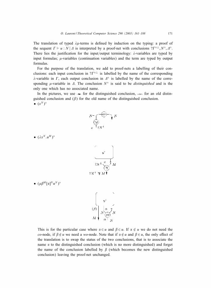
The translation of typed ��-terms is de.ned by induction on the typing: a proof ofthe sequent � � u : N |" is interpreted by a proof-net with conclusions ?�◦⊥; N ◦; "◦.There lies the justi.cation for the input=output terminology: �-variables are typed byinput formulas; �-variables (continuation variables) and the term are typed by outputformulas.For the purpose of the translation, we add to proof-nets a labelling of their con-

clusions: each input conclusion in ?�◦⊥ is labelled by the name of the corresponding�-variable in �, each output conclusion in "◦ is labelled by the name of the corre-sponding �-variable in ". The conclusion N ◦ is said to be distinguished and is theonly one which has no associated name.In the pictures, we use for the distinguished conclusion, for an old distin-

guished conclusion and (�) for the old name of the distinguished conclusion.• (xN )◦

• (�xN :uM )◦

• (��M [�]NuN )◦

This is for the particular case where �∈ u and �∈ u. If � =∈ u we do not need theco-node, if � =∈ u we need a wo-node. Note that if � =∈ u and �∈ u, the only e3ect ofthe translation is to swap the status of the two conclusions, that is to associate thename � to the distinguished conclusion (which is no more distinguished) and forgetthe name of the conclusion labelled by � (which becomes the new distinguishedconclusion) leaving the proof-net unchanged.


• ((uN →M )vN )◦

We can separate in two parts the case of ��[�]u if we translate named terms [�]uas proof-nets without distinguished conclusion. The [�] construction on u introduces acontraction node if �∈ u. The �� construction introduces a weakening node if � =∈ u.Another way to deal with named terms is to put explicitly the type ⊥. The two

�-rules become

V � u : N |"V � [�]u : ⊥ | � : N; "

�-name′;

V � [�]u : ⊥ | � : M;"V � ��[�]u : M |" �-abs′:

These two rules can be translated into proof-nets 2 through the translation ()�:

• ([�]NuN )�

• (��M :u⊥)�

2 The introduction of 1- and ⊥-nodes does not modify the correctness criterion.


The translation ()� is the same as ()◦ for the other rules. We can recover ()◦ from()� by reducing the cuts on constants. Indeed, by de.nition of ��-calculus, �� and [�]always come together, so the constant cuts are always between 1-nodes and ⊥-nodeswhich vanish by reduction.The ()� translation allows to account with a slight generalization of ��-calculus with

a new rule for ⊥ corresponding to the construction ��M :u⊥ for any u of type ⊥ (notonly named terms). In this case 1-nodes are not always cut against ⊥-ones. Since ⊥is an output formula, the ⊥-node is just a particular case of the wo-node. On the otherhand, the 1-node introduces a new kind of leaves for ⊗-trees.With this extension, we can, for example, translate the C operator of Felleisen of

type ¬¬N →N de.ned in ��-calculus by �f¬¬N :��N :(f)�xN : [�]N x:

2.3. Simulation of reduction

The translation ()◦ has also a dynamic meaning: it simulates ��-reduction by cutelimination in proof-nets.Until the end of the paper, we have to identify all the binary trees of contractions

with the same number of nodes, the sequence w–c with a simple edge and a co-nodeon two input conclusions of a box with the same node inside the box. Another solutionhas been proposed in [2, 12] to get rid of this problem with generalized contractions.Final w-nodes of a proof-net correspond to variables in the context not free in the

term. As done for typing derivations, we want to ignore them. In the sequel we willnot care about such .nal w-nodes. In particular we say that two proof-nets are equalif they di3er only by .nal w-nodes. This is the counterpart of the fact that, in varioussystems, two typing proofs that di3er only in useless variable declarations may beconsidered equal.


Lemma 18 (�-Substitution). Modulo 4nal w-nodes and structure of contraction trees:

Lemma 19 (�-Substitution). Modulo 4nal w-nodes and structure of contraction trees:

Proof. These two lemmas are proved by induction on u.

Theorem 20 (Simulation). If u→ v then u◦ →∗ v◦.

Proof. We just have to apply Lemmas 18 and 19. In the case of �-reduction, thesimulation is strict: one step in ��-calculus corresponds to at least one step in proof-nets. On the other hand, a �-reduction may be translated by identity, typically in thecase: (��[�]u)v →� ��[�](u)v with � =∈ u.

Remark 21. Due to the �-equivalence (next section), we cannot hope for any converseresult. For example, if u= � [�]�x:��′[�]�y:(��′[ ](y)x)t and v= � [�]�y:��′[�]�x:��′

[ ](y)x, u◦ →∗ v◦ but v is not a reduct of u.

We now consider proof-nets up to multiplicative (i.e. ⊗=o and ax) reductions. Thejusti.cation for doing so is that these reductions are operationally simple: they strictlydecrease the size of the net and they are local, so that the heart of the dynamics maybe thought of as lying in structural reductions.

De�nition 22 (Translation ()•). The translation u• of a ��-term u is the multiplicativenormal form of the proof-net u◦.

Remark 23. We have de.ned three translations with the following relations:

u�1=⊥−→ u◦

⊗=o;ax−→ u•:


With the translation ()•, the last theorem is no longer correct, for example:

((��:u)v1)v2 →� (��:u[[�](w)v1=[�]w])v2 →� ��:u[[�](w)v1v2=[�]w]

but in the corresponding proof-net (((��:u)v1)v2)• these two steps are done in just one,so that the translation of the middle term is not reachable from the translation of the .rstone. Asking for “consecutive” �-redexes to be reduced in one step by modifying the�-reduction: (��:u)v1 : : : vn →�′ ��:u[[�](w)v1 :::vn =[�]w] (where (��:u)v1 : : : vn is not ap-plied to another term vn+1) does not solve the problem since as shown in the followingexample the sequence v1 : : : vn may be hidden in the ��-term:

((�x:(��:u)v1)t)v2 →�′ ((�x:��:u[[�](w)v1=[�]w])t)v2

→� (��:u[[�](w)v1=[�]w][t =x])v2 →�′ ��:u[[�](w)v1v2=[�]w][t =x]:

On the other hand ()• translates normal terms as cut-free proof-nets, �-redexes as !=?cuts and �-redexes as ⊗=co; ⊗=wo or ⊗=! cuts (except in some particular cases like(��[�]x)v).

2.4. Sequentialization

We now address the question of surjectivity of the translation ()•.

De�nition 24 (��-Proof-structure). A ��-proof-structure is a proof-structure with nopositive conclusion, no .nal wi-node and only structural cuts.

The “no 4nal wi-node” constraint is not needed for Theorem 30 if we want to sequen-tialize proof-nets as typing derivations with explicit structural rules because they justadd variables in the context not free in the ��-term (see p. 14).

Remark 25. When a proof-structure has no positive conclusion, the correctness condi-tion on the number of ?d-nodes can be replaced by: exactly one dereliction at depth0 and in each box.

Lemma 26. Let R be a proof-structure with a 4nal negative node n; R\n is thegraph obtained from R by erasing the node n. Then R\n is a proof structure and ifR is correct; R\n is correct.

Lemma 27. Let u be a term with two free �- (resp. �-) variables x1 and x2 (resp. �1and �2); (u[x=x1 ;

x=x2 ])• (resp. (u[�=�1 ;

�=�2 ])•) is obtained from u• by adding a ci-node

(resp. co-node) between the two conclusions corresponding to x1 and x2 (resp. �1 and�2).

Lemma 28. Let R be a cut-free proof-net; if e is a negative edge either it is aconclusion of R or moving downward from e yields to a 4nal negative node.


Lemma 29. Let R be a proof-net without any 4nal negative node. If c is a maxi-mal 3 cut-node in R then c is splitting; that is R is obtained by cutting the negativeconclusion A of a proof-net R− with the positive conclusion A⊥ of a proof-net R+.Furthermore R+ is a ⊗-tree.

Proof. The last four results are immediate.

Theorem 30 (Sequentialization). A proof-structure with a distinguished conclusion isthe translation ()• of a ��-term if and only if it is a ��-proof-net.

Proof. The “only if” part is immediate. Conversely, we sequentialize any ��-proof-net R with a distinguished conclusion as a ��-term. We start by associating distinct�-variables to input conclusions and distinct �-variables to output conclusions of R.We then sequentialize R as a named term [�]u and we de.ne the complete sequential-ization of R to be ��[�]u where � is the name associated to the distinguished outputconclusion. The construction of [�]u is done by induction on R:• If R has a .nal o-node n whose conclusion ?N⊥oM has name �, let u be asequentialization of R\n (or of (R\n)\n′ if ?N⊥ is introduced by a wi-node n′)with names x for ?N⊥ and � for M . We sequentialize R as [�]N→M�xN :��M :u.

• If R has a .nal co-node n whose conclusion N has name �, let u be a sequential-ization of R\n with names �1 and �2 for the premises N of n. We sequentialize R

as u[�=�1 ;�=�2 ] by Lemma 27.

• If R has a .nal wo-node n whose conclusion N has name �, let u be a sequential-ization of R\n. We sequentialize R as [�]N�%N :u where % does not occur in u.

• If R has a .nal co-node n whose conclusion ?N⊥ has name x, let u be a sequential-ization of R\n with names x1 and x2 for the premises ?N⊥ of n. We sequentializeR as u[x=x1 ;

x=x2 ] by Lemma 27.• If R has no .nal negative node, we consider a maximal cut-node which is splittingby Lemma 29. Let R− (resp. R+) be the proof-structure above its negative (resp.positive) premise. By Lemma 29, R+ is a ⊗-tree. We have two cases dependingon the type of the cut formula:◦ if it is an input formula ?N⊥, we sequentialize R− (or R−\n′ if ?N⊥ is intro-duced by a wi-node n′) with name x for the conclusion ?N⊥ as u. Since the rootof R+ is !N; R+ must be 4at, i.e R+ is a box B associated to a !-node. Letv be the complete sequentialization of B (whose conclusion N is distinguishedand whose other conclusions are named as in R). We pick an output conclusionof R− (it must have one by the fourth remark in Section 1.2) with name �. Wesequentialize R as [�]M (�xN :��M :u)vN ;

◦ if it is an output formula N , let u be the sequentialization of R− with the newname � associated to its conclusion N and v1; : : : ; vn be the complete

3 see Section 1.2.


sequentializations of the boxes associated to the !-leaves of R+. If � is the nameof the main conclusion 4 of the ⊗-tree R+, we sequentialize R as [�]N (��N :u)v1: : : vn.

• If R has no .nal negative node and no cut at depth 0, then let n be its maininitial node which is a ?d-node by the remark above. Then the conclusion of n isa conclusion of R by Lemma 28. Furthermore its premise is the root of a ⊗-treeR+ and the conclusions of R+ are conclusions of R by Lemma 28, i.e. R+ =R\n.If the conclusion ?M⊥ of n has name x and the main conclusion N of R+ hasname �, we sequentialize R as [�]N (xM )v1 : : : vn where v1; : : : ; vn are the completesequentializations of the boxes associated to the !-leaves of R+.

One may check that in each case the translation ()• applied to the constructed termyields the original proof-net (up to associativity of contractions, commutations ofauxiliary doors with contractions and neutrality of weakening w.r.t. contractions, asexplained above).

Remark 31.• Maximal cut-nodes correspond to leftmost redexes in ��-calculus. The translationof the leftmost redex of a ��-term is a maximal cut-node and conversely if c is amaximal cut-node, there exists a ��-term such that its leftmost redex is translatedas c.

• The dereliction at depth 0 corresponds to the head variable of the term. If theconclusion of this node is a conclusion of the proof-net it means that the headvariable of the ��-term is free and linear.

This sequentialization procedure yields ��-terms with a particular shape: ��[�] con-structions surround each �-abstraction, each application; : : : The �-equivalence will showthat this kind of ��-terms is not so peculiar because there exists at least one such termin each �-equivalence class.

3. The �-equivalence

We characterize now the identi.cation between ��-terms induced by the translation.The answer has already been given for the �-calculus in [12, 13] as the �-equivalence.We give here a “conservative” extension of this equivalence on ��-terms. However thisextension has a very di3erent behavior on ��-terms. The �-equivalence of �-calculusis de.ned in terms of commutations of redexes, in particular a normal term is onlyequivalent to itself, but here the (pop=pop) equation provides identi.cations betweennormal terms. We will also see a normal term equivalent to a non-normal one.

4 see Section 1.3.


3.1. De4nition

De�nition 32 (Atomic contexts). An atomic context C0 is obtained by applying oneof the constructions of the ��-calculus to a hole instead of a term:

C0 ::= �y:[ ] | � [�][ ] | ([ ])u:

An atomic named context N0 is constructed in the same way but with named terms:

N0 ::= [�]�y:� :[ ] | [�](� :[ ])u:

We say that � (resp. x) is bound in C0 if � =∈C0[�%[�]x] (resp. x =∈C0[x]). We say thatC0 is �-free (resp. x-free) if � (resp. x) =∈C0 and if � (resp. x) is not bound in C0.And we use the same terminology for N0.

De�nition 33 (�-Equivalence). The �-equivalence is the smallest compatible (i.e. pre-served by abstractions and application) equivalence relation on ��-terms containing:• generalization of �-equivalence on �-calculus for commutation of �-redexes with allthe constructions of ��-calculus,

((�x:u)v)w ∼� (�x:(u)w)v x =∈ w; (�1)

(�x:�y:u)v ∼� �y:(�x:u)v{

x �= y;y =∈ v;

(�2)

(�x:��[�]u)v ∼� ��[�](�x:u)v � =∈ v; (�3)

• particular ��-features giving new commutations,

[�′](��[�′](��:u)v)w ∼� [�′](��[�′](��:u)w)v{

� =∈ v;� =∈ w;

(push=push)

[�′]�x:��[�′]�y:��:u ∼� [�′]�y:��[�′]�x:��:u x �= y; (pop=pop)

[�′](��[�′]�x:��:u)v ∼� [�′]�x:��[�′](��:u)v{

x =∈ v;� =∈ v;

(push=pop)

with � �= �, � �= �′ and �′ �= � in these three equations.• usual '- and (-reductions of ��-calculus

[�]��:u ∼� u[�=�]; (')

��[�]u ∼� u; � =∈ u: (()

The '-reduction (resp. (-reduction) is obtained by orienting (') (resp. (()) from theleft-hand side to the right-hand side.These equations (except (') and (()) can also be factorized through the notion of

atomic context:

C0[(�x:u)v] ∼� (�x:C0[u])v; (�i)


where C0 is x-free and no free variable of v is bound in C0,

N0[N ′0[u]] ∼� N ′

0[N0[u]]; (p=p)

where if � (or x) is bound in N0 (resp. N ′0) then N ′

0 (resp. N0) is �-free (or x-free).

We may justify these equations operationally by examining their behavior withinKrivine’s abstract machine [6]. Approximatively a state of this machine is a triple(t; e; s) where t is a term, e is an environment containing associations (�-variable, term)and (�-variable, stack) and s is a stack, that is a sequence of terms. The transitionsare:(jump) If t is a variable x, proceed with its value as de.ned in e.(push) If t is an application (u)v, the argument v is pushed onto the stack and the

machine proceeds with u.(pop) If t is a �-abstraction �x :u, the .rst element of the stack is popped and stored

with name x in the environment and the machine proceeds with u.(store) If t is a �-abstraction ��:u, the stack is stored under the name � in the

environment and execution continues with u and the empty stack *.(restore) If t is a named term [�]u, the stack is replaced by a copy of the

one associated to � in the environment and execution proceeds with u and the newstack.We can, for example, describe the case of (push=pop) (which should enlighten its

name). If we start with the state ([�′](��[�′]�x :��:u)v; e; *) where e contains the associ-ations: (�′; s1) and (�′; w :: s2), the machine goes through the followingsteps:• restore the stack s1;• push v on s1;• store the new stack v :: s1 with name �;• restore the stack w :: s2;• pop w and store it with name x;• save the popped stack s2 with name �.The machine reaches the state (u; e′; *) where e′ is e augmented with the associ-ations (�; v :: s1), (x; w) and (�; s2). One easily checks that starting with the state([�′]�x:��[�′](��:u)v; e; *), the machine goes through the same steps.

3.2. Properties of the �-equivalence

Proposition 34. Let u and v be two ��-terms; if u∼� v then u∼� �'( v.

Proof. We prove that each equation of the �-equivalence is realized by the � �'(-equivalence:• (�1), (�2) and (�3) are realized by the �-equivalence;• (push=push) and (push=pop) are realized by the �'-equivalence;


• for the (pop=pop) equation we .rst show the following equivalence which corre-sponds to the (S3) rule in [10]:

��′ : : : [�′]�x:��:t : : : ∼ �x:(��′ : : : [�′]�x:��:t : : :)x ( )∼ �x:��′ : : : [�′](�x:��:t)x : : : (�)∼ �x:��′ : : : [�′]��:t : : : (�)∼ �x:��′ : : : t[�

′=�] : : : ; (')

where the �-reduction also substitutes the other sub-terms [�′]u by [�′](u)x. If weapply two '-expansions in each member of the (pop=pop) equation we obtain

[�′]��′[�′]��′[�′]�x:��[�′]�y:��:u

and

[�′]��′[�′]��′[�′]�y:��[�′]�x:��:u

and by applying the above equation twice to each term we get the same one

[�′]�x:��′[�′]�y:��′u[�′=�; �

′=�]:

This shows that (pop=pop) is realized by the � �'-equivalence.• (') and (() are realized by the '(-equivalence.

Proposition 35 (Preservation properties). Let u and v be two ��-terms such thatu∼� v.• If u is normalizable then v is normalizable and their normal forms are �-equivalent.• If u has a head normal form 5 then v has a head normal form.• If u is strongly normalizable then v is strongly normalizable.• If u is typable of type A then v is typable of type A.

Proof. All these properties are in fact corollaries of Theorem 4:1.

Let us look at the kind of transformations of typing derivations realized by the�-equivalence, for example with the (push=pop) equation. If �; x :A � u | � :C→D; � :B; " and �′ � v :C |"′, we have:

�; x :A� u | � :C→D; � :B; "�-abs,

�; x :A� ��:u :B | � :C→D;"abs,

� � �x:��:u :A→B | � :C→D;"�;

� � ��[�′]�x:��:u :C→D | �′ :A→B; " �′ � v :C |"′app,

�; �′ � (��[�′]�x:��:u)v :D | �′ :A→B; "; "′�-name

�; �′ � [�′](��[�′]�x:��:u)v | �′ :D; �′ :A→B; "; "′

5 It is the natural generalization of the notion of head normal forms for the �-calculus, see [4] for a precisede.nition.


and

�; x :A� u | � :C→D; � :B; "�-abs,

�; x :A� ��:u :C→D | � :B; " �′ � v :C |"′app,

�; �′; x :A� (��:u)v :D | � :B; "; "′�;

�; �′; x :A� ��[�′](��:u)v :B | �′ :D;"; "′abs,

�; �′ � �x:��[�′](��:u)v :A→B | �′ :D;"; "′�-name.

�; �′ � [�′]�x:��[�′](��:u)v | �′ :D; �′ :A→B; "; "′

The �-equivalence realizes complex identi.cations in particular between normal andnon-normal terms even if we consider normal terms modulo '- and (-reductions: lett be a closed term and u= �x:��[�](��[�]�y:�%[�]x)t, v= �x:��[�]�y:�%[�](x)t, wehave u∼� v (this is in fact a variant of (push=pop) and a particular case of Lemma 39)but also u→+ v:

u →� �x:��[�]��[�]�y:�%[�](x)t →' v:

Thus there is no hope that �-equivalence preserves length of reduction as it does in�-calculus. The reason is that ��-calculus contains linear �-redexes which have no realoperational meaning. More precisely, we are now going to show that the �-equivalenceidenti.es terms which di3er only by linear �-redexes.

De�nition 36 (Contexts). A context C is a term, with a hole in place of a sub-term,de.ned in the following way:

C ::= [ ] | �y:C | � [�]C | (C)u:A named context N is a named term, with a hole in place of a named sub-term:

N ::= [ ] | [�]C[� :[ ]]:The notions of variable bound in a context and of �-free and x-free contexts are thesame as for atomic contexts.

De�nition 37 (Linear �-redex). A �-redex occurring in a ��-term is linear if it hasthe shape (��:N [[�]u])v where N is an �-free named context and � =∈ u. The size ofthe �-redex is the size of the term ��:N [[�]u].

Lemma 38 (Pop out). If N is x- and �′-free; � not bound in N and �′ =∈ u:

N [[�]�x:u] ∼� [�]�x:��′:N [[�′]u]:

Proof. By induction on N :• If N = [ ]:

[�]�x:u ∼� [�]�x:��′[�′]u (()


• If N = [�]� : [ ]:

[�]� [�]�x:u ∼� [�]� [�]�x:��′[�′]u (()

∼� [�]�x:��′[�′]u[�= ] (')

∼� [�]�x:��′[�]� [�′]u: (')

• If N = [�]�y:C[� :[ ]]:

[�]�y:C[� :[�]�x:u] ∼� [�]�y:��′[�′]C[� :[�]�x:u] (()

∼� [�]�y:��′[�]�x:��′[�′]C[� [�′]u] by induction

∼� [�]�x:��′[�]�y:��′[�′]C[� [�′]u] (pop=pop)

∼� [�]�x:��′[�]�y:C[� [�′]u]: (()

• If N = [�]��′[ ′]C[� : [ ]]:

[�]��′[ ′]C[� [�]�x:u] ∼� [�]��′[�]�x:��′[ ′]C[� [�′]u] by induction

∼� [�]�x:��′[ ′]C[� [�′]u][�=�′ ] (')

∼� [�]�x:��′[�]��′[ ′]C[� [�′]u]: (')

• If N = [�](C[� : [ ]])v:

[�](C[� [�]�x:u])v ∼� [�](��′[�′]C[� [�]�x:u])v (()

∼� [�](��′[�]�x:��′[�′]C[� [�′]u])v by induction

∼� [�]�x:��′[�](��′[�′]C[� [�′]u])v (push=pop)

∼� [�]�x:��′[�](C[� [�′]u])v: (()

Lemma 39 (Push out). If N is �′-free; if � is not bound in N; if �′ =∈ u and if noneof the free variables of v is bound in N :

N [[�](u)v] ∼� [�](��′:N [[�′]u])v:

In particular linear �-reduction is included in �-equivalence.

Proposition 40 (Elimination of linear �-redexes). Let u be a ��-term; there exists u′

such that u′ ∼� u and u′ has no linear �-redex.

In particular linear �-reduction terminates.

Proof. We prove that each linear �-redex can be replaced by a smaller �-redex oreliminated:

(��:N [[�]u])v ∼� ��[�](��:N [[�]u])v (()

∼� ��:N [[�](u)v] by Lemma 39:


3.3. Completeness of the �-equivalence

Theorem 41. Let t and t′ be two ��-terms; t•= t′• ⇔ t∼� t′.

Proof. Let t and t′ be two �-equivalent terms, we have to show that they have thesame translations. To do this we just look at the proof-nets corresponding to the eightequations of �-equivalence:(�1) By multiplicative reductions, (((�x:u)v)w)◦ and ((�x:(u)w)v)◦ yield the same

proof-net:

which eventually gives t•= t′• by ending the multiplicative reduction.(�2) In the same way, by multiplicative reductions from ((�x :�y:u)v)◦ and (�y:(�x :u)

v)◦, we obtain the proof-net:

(�3) Idem with ((�x :��[�]u)v)◦ and (��[�](�x :u)v)◦.


(push=push) The terms ([�′](��[�′](��:u)v)w)◦ and ([�′](��[�′](��:u)w)v)◦ imme-diately give the same proof-net:

(pop=pop) Idem with ([�′]�x :��[�′]�y:��:u)◦ and ([�′]�y:��[�′]�x :�� :u)◦.

(push=push) Idem with ([�′](��[�′]�x :��:u)v)◦ and ([�′]�x :��[�′](��:u)v)◦.

The last two cases are even simpler so we skip them.

For the converse we need some new lemmas.

Lemma 42. Let [�]u be a named term containing a free �-variable � such that theconclusion corresponding to � in ([�]u)• is neither an auxiliary door of a box northe conclusion of a co-node. There exist an �-free context N and a ��-term u1 suchthat [�]u=N [[�]u1] with � =∈ u1.

Proof. If �= � then � =∈ u (otherwise we would have a contraction above the conclusioncorresponding to � in ([�]u)•) and the result is proved with N = [ ]. If � �= � we prove


the lemma by induction on u:• If u= x then �= �.• If u= �x :u′ then [�]u′ veri.es the same hypothesis as [�]u thus, by induction hy-pothesis, [�]u′=N [[�]u1] with N �= [ ] since � �= �. We have N = [�]C[� : [ ]] and[�]u= [�]�x :C[� [�]u1].

• If u= � [ ′]u′ then �= � (otherwise � =∈ [�]u). If ′= � we have N = [�]� : [ ]. If ′ �= �, [�]u′ veri.es the same hypothesis as [�]u and, by induction, [�]u′=N [[�]u1]with N �= [ ] thus N = [�]C[��′: [ ]] and [�]u= [�]� [ ′]C[��′[�]u1].

• If u=(u′)v then � is not free in both u′ and v otherwise the corresponding conclusionof ([�]u)• would be conclusion of a co-node and � =∈ v otherwise it would be anauxiliary door of a box. [�]u′ veri.es the same hypothesis as [�]u and, by induction,[�]u′=N [[�]u1] with N �= [ ] thus N = [�]C[� : [ ]] and [�]u= [�](C[� [�]u1])v.

Lemma 43. If u• has a 4nal o-node n:• if n is above the distinguished conclusion then there exists a term u′ such that

u∼� �x :u′;• if n is above another conclusion then there exists a term u′ such that u∼� ��[�]

�x :u′.

Proof. We begin with the second point which is an easy consequence of the .rstone. Let � be the name of (the conclusion of) n and consider the term v= ��[�]u(� =∈ u). By de.nition of the translation, v• is the same proof-net as u• but has nas distinguished conclusion. By the .rst case, we obtain u′ such that v∼� �x :u′. Thus��[�]��[�]u∼� ��[�]�x :u′; furthermore ��[�]��[�]u∼� u by (') and (() because � =∈ uso that u∼� ��[�]�x :u′.We now turn to the .rst point which is proved by induction on the term u:

(1) If u= x then the distinguished conclusion must be the conclusion of an axiomnode, a contradiction.

(2) If u= �x :u0, the result is proved.(3) If u= ��[�]u0 then �∈ [�]u0 since the distinguished conclusion of u• is not below

a wo-node. By Lemma 42, we have u= ��:N [[�]u1] where N is an �-free contextand � =∈ u1. By induction hypothesis, u1∼� �x :u′ and by Lemma 38,

u∼� ��:N [[�]�x :u′]

∼� ��[�]�x:��′:N [[�′]u′]

∼� �x:��′N [[�′]u′]:

(4) If u=(u0)v1 : : : vn where n¿0 and u0 is not an application, we look at the di3erentcases for u0:(a) u0 = x, impossible as for 1.(b) u0 = �x :u1 then ((u1)v2 : : : vn)• is a sub-proof-net of u• which has the same

.nal o-node. By induction hypothesis: (u1)v2 : : : vn ∼� �y:u′ (with y chosen


not free in v1) so

u = (�x:u1)v1 : : : vn∼� (�x:(u1)v2 : : : vn)v1 (�1)

∼� (�x:�y:u′)v1∼� �y:(�x:u′)v1 (�2)

(c) u0 = ��[�]u1 then u• is obtained by the multiplicative reduction of a cutbetween u•0 and the non4at ⊗-tree containing the v•i ’s. If the node abovethe distinguished conclusion of u•0 is not a o-node or an ax-node, this cutcannot be multiplicatively reduced and the distinguished conclusion of u• isthe main conclusion of the ⊗-tree which contradicts our hypothesis that it isconclusion of the o-node n. By Lemma 42, u0 = ��:N [[�]u2] where N is an�-free context and � =∈ u2. We use Lemma 39:

u = (��:N [[�]u2])v1 : : : vn∼� � [ ](��:N [[�]u2])v1 : : : vn∼� � :N [[ ](u2)v1 : : : vn]

then by induction hypothesis (u2)v1 : : : vn ∼� �x :u′ and by Lemma 38:

u∼� � :N [[ ]�x:u′]

∼� � [ ]�x:��:N [[�]u′]

∼� �x:��:N [[�]u′]:

Lemma 44. If u• has no 4nal negative node and has a maximal cut-node with anon:at ⊗-tree above it; there exist u′; v1; : : : ; vn such that:• if the main conclusion of the ⊗-tree is distinguished then we have u∼� (��[�]u′)

v1 : : : vn;• if the main conclusion of the ⊗-tree is not distinguished then we have u∼� ��′[�′](��[�]u′)v1 : : : vn.

Lemma 45. If u• has no 4nal negative node and has a maximal cut-node with a :at⊗-tree above it then there exist u′ and v such that u∼� (�x :u′)v.

We are now able to .nish the proof of Theorem 41.

Proof (Theorem 41—continued): By induction on t•, following the proof of Theo-rem 30:• If t• has a .nal o-node n above the distinguished conclusion, by Lemma 43,

t∼� �x: t0 and t′ ∼� �x: t′0. By de.nition of the translation t•0 = t•\n= t′•\n= t′•0 , thust•0 = t′•0 , by induction hypothesis t0∼� t′0 and t∼� t′.


• If t• has a .nal o-node n above another conclusion, by Lemma 43, t∼� ��[�]�x: t0and t′ ∼� ��[�]�x: t′0 so that t

•0 = t•\n= t′•\n= t′•0 thus by induction hypothesis t0∼�

t′0 and t∼� t′.• If t• has a .nal co-node or a .nal wo-node it is very similar.• If t• has a .nal ci-node n with name x, let t0 (resp. t′0) be a term with two freevariables x1 and x2 such that t•0 = t•\n (resp. t′•0 = t′•\n) where x1 and x2 are thenames of the premises of n and such that t0[x=x1 ;

x=x2 ] = t (resp. t′0[x=x1 ;

x=x2 ] = t′). Byinduction t0∼� t′0 thus we have t∼� t′.

• t• cannot have a .nal wi-node.• If t• has no .nal negative node but some cut-nodes, let c be a maximal one. If the

⊗-tree above the positive premise of c is not 4at we apply Lemma 44. If it is 4atwe apply Lemma 45.

• If t• has no .nal negative node and no cut then t∼� (x)u1 : : : un and t′ ∼� (x)v1 : : : vnwith ui ∼� vi by induction hypothesis inside boxes thus t∼� t′.

4. Pure case

Considering pure proof-nets corresponds to applying the recursive equation N = !N (N on types. This identi.es all output formulas and gives exactly four types: O (outputformulas) and its dual I (anti-output formulas); ?I (input formulas) and its dual !O(anti-input formulas).

where A is either O or ?I .The translations studied before can be seen as translations of pure ��-calculus into

pure polarized proof-nets extending those for �-calculus in [1, 12].All the results are still valid except, of course, strong normalization (Corollary 15).

In particular:

Proposition 46 (Con4uence). The reduction of pure polarized proof-nets is con:uent.

Proposition 47 (�-equivalence). Let t and t′ be two pure ��-terms; then t•= t′• ⇔t∼� t′.


Acknowledgements

I would like to thank V. Danos for the key question of Section 3 and L. Regnierfor personal and mathematical help and support. Thanks also to the referee for theimportant comments and suggestions he made.

References

[1] V. Danos, La logique linWeaire appliquWee Xa l’Wetude de divers processus de normalisation (principalementdu �-calcul), ThXese de doctorat, UniversitWe Paris VII, 1990.

[2] V. Danos, L. Regnier, Proof-nets and the Hilbert space, in: J.-Y. Girard, Y. Lafont, L. Regnier (Eds.),Advances in Linear Logic, London Mathematical Society Lecture Note Series, Vol. 222, CambridgeUniversity Press, Cambridge, 1995, pp. 307–328.

[3] V. Danos, J.-B. Joinet, H. Schellinx, A new deconstructive logic: linear logic, J. Symbolic Logic 62(3) (1997) 755–807.

[4] R. David, W. Py, ��-calculus and BPohm’s theorem, J. Symbolic Logic 66 (1) (2001) 407–413, URLftp:==www.lama.univ-savoie.fr=pub=users=DAVID=bohm.ps.

[5] J.-Y. Girard, A new constructive logic: classical logic, Math. Struct. Comput. Sci. 1 (3) (1991)255–296.

[6] J.-L. Krivine, Un interprWeteur du lambda-calcul, unpublished. URL ftp:==ftp.logique.jussieu.fr=pub=distrib=krivine=interprt.pdf.

[7] O. Laurent, Logique linWeaire polarisWee et logiques classiques, MWemoire du magistXere M.M.F.A.I.,Ecole Normale SupWerieure de Paris, September, 1999. URL ftp:==iml.univ-mrs.fr=pub=olaurent=mmfai.ps.gz.

[8] O. Laurent, Polarized proof-nets: proof-nets for LC (extended abstract), in: J.-Y. Girard (Ed.), TypedLambda Calculi and Applications ’99, Lecture Notes in Computer Science, Vol. 1581, Springer, Berlin,1999, pp. 213–227.

[9] M. Parigot, ��-calculus: an algorithmic interpretation of classical natural deduction, in: Proc. Internat.Conf. on Logic Programming and Automated Deduction, Lecture Notes in Computer Science, Vol. 624,Springer, Berlin, 1992, pp. 190–201.

[10] M. Parigot, Classical proofs as programs, in: Proceedings of Kurt GPodel Colloquium, Lecture Notes inComputer Science, Vol. 713, Springer, Berlin, 1993, pp. 263–276.

[11] M. Quatrini, L. Tortora de Falco, Polarisation des preuves classiques et renversement, Compte-Rendude l’AcadWemie des Sciences de Paris 323 (1996) 113–116.

[12] L. Regnier, Lambda-calcul et rWeseaux, ThXese de doctorat, UniversitWe Paris VII, 1992.[13] L. Regnier, Une Wequivalence sur les lambda-termes, Theoret. Comput. Sci. 126 (1994) 281–292.[14] P. Selinger, Control categories and duality: on the categorical semantics of the lambda-mu calculus,

Math. Struct. Comput. Sci. 11 (2) (2001) 207–260, URL ftp:==ftp.math.lsa.umich.edu=pub=selinger=control.ps.gz.

Polarized proof-nets and λμ-calculus

Documents

Transcript of Polarized proof-nets and λμ-calculus