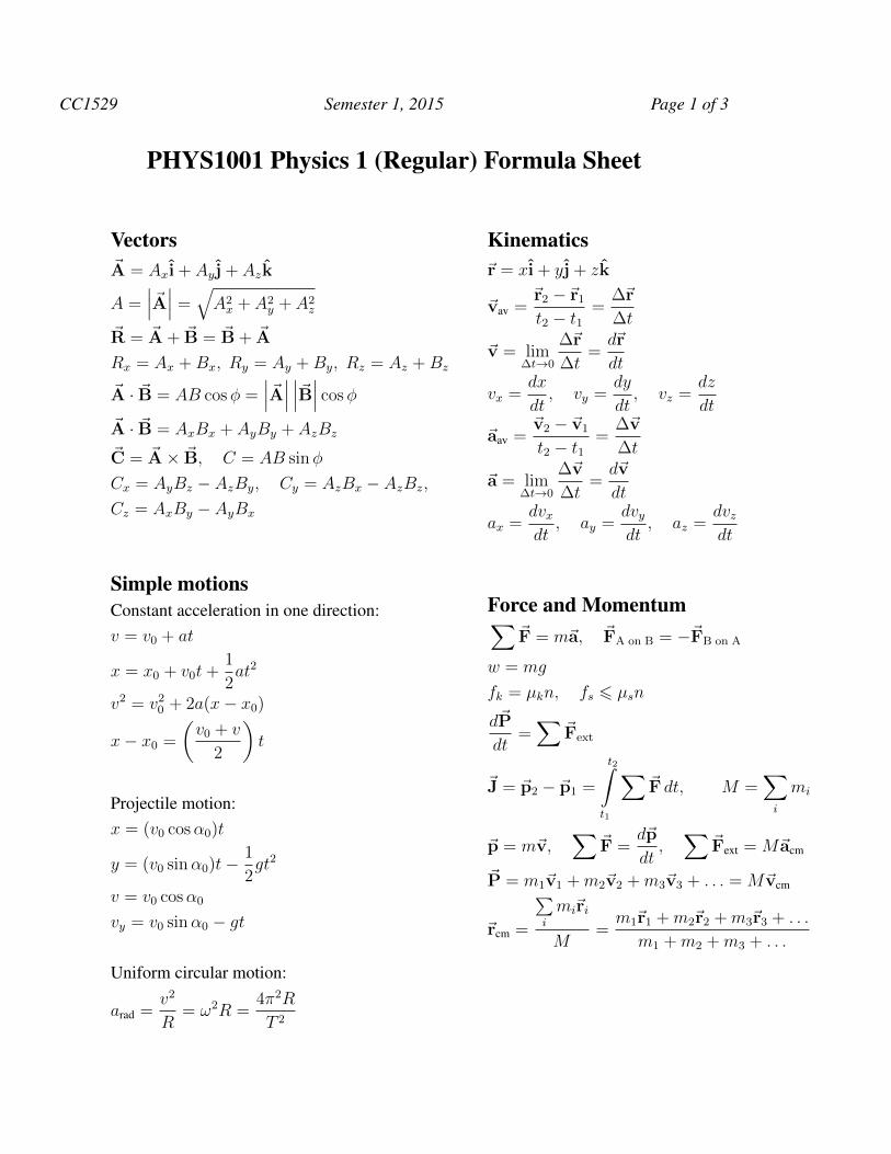
CC1529 Semester 1, 2015 Page 1 of 3

PHYS1001 Physics 1 (Regular) Formula Sheet

Vectors~A = Axi+ Ay j+ Azk

A =

���~A��� =

qA2

x + A2

y + A2

z

~R =

~A+

~B =

~B+

~A

Rx = Ax +Bx, Ry = Ay +By, Rz = Az +Bz

~A · ~B = AB cos� =

���~A������~B

��� cos�~A · ~B = AxBx + AyBy + AzBz

~C =

~A⇥ ~B, C = AB sin�

Cx = AyBz � AzBy, Cy = AzBx � AzBz,

Cz = AxBy � AyBx

Simple motionsConstant acceleration in one direction:v = v

0

+ at

x = x0

+ v0

t+1

2

at2

v2 = v20

+ 2a(x� x0

)

x� x0

=

✓v0

+ v

2

◆t

Projectile motion:x = (v

0

cos↵0

)t

y = (v0

sin↵0

)t� 1

2

gt2

v = v0

cos↵0

vy = v0

sin↵0

� gt

Uniform circular motion:

arad =v2

R= !2R =

4⇡2R

T 2

Kinematics~r = xi+ yj+ zk

~vav =~r2

�~r1

t2

� t1

=

�

~r

�t

~v = lim

�t!0

�

~r

�t=

d~r

dt

vx =

dx

dt, vy =

dy

dt, vz =

dz

dt

~aav =~v2

� ~v1

t2

� t1

=

�

~v

�t

~a = lim

�t!0

�

~v

�t=

d~v

dt

ax =

dvxdt

, ay =dvydt

, az =dvzdt

Force and MomentumX

~F = m~a, ~FA on B

= �~FB on A

w = mg

fk = µkn, fs 6 µsn

d~P

dt=

X~F

ext

~J =

~p2

� ~p1

=

t2Z

t1

X~F dt, M =

X

i

mi

~p = m~v,X

~F =

d~p

dt,

X~Fext = M~acm

~P = m1

~v1

+m2

~v2

+m3

~v3

+ . . . = M~vcm

~rcm =

Pi

mi~ri

M=

m1

~r1

+m2

~r2

+m3

~r3

+ . . .

m1

+m2

+m3

+ . . .

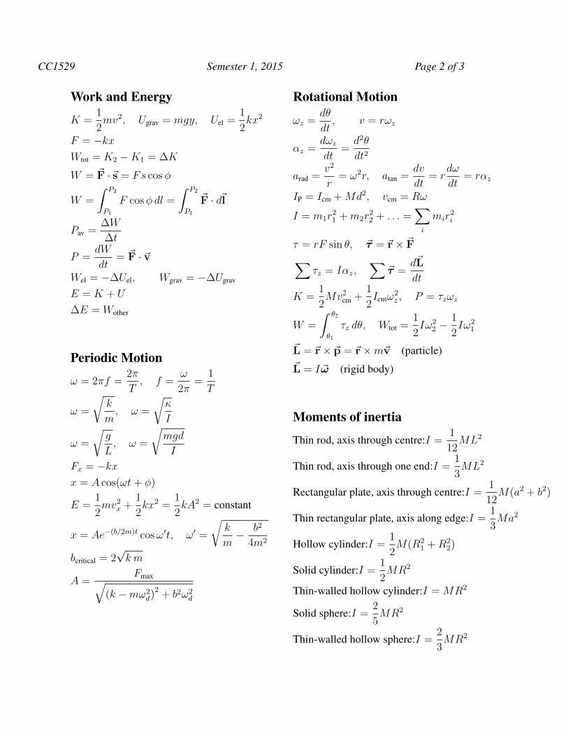
CC1529 Semester 1, 2015 Page 2 of 3

Work and Energy

K =

1

2

mv2, Ugrav = mgy, Uel =1

2

kx2

F = �kx

Wtot = K2

�K1

= �K

W =

~F ·~s = Fs cos�

W =

Z P2

P1

F cos� dl =

Z P2

P1

~F · d~l

Pav =�W

�t

P =

dW

dt=

~F · ~v

Wel = ��Uel, Wgrav = ��Ugrav

E = K + U

�E = Wother

Periodic Motion

! = 2⇡f =

2⇡

T, f =

!

2⇡=

1

T

! =

rk

m, ! =

r

I

! =

rg

L, ! =

rmgd

I

Fx = �kx

x = A cos(!t+ �)

E =

1

2

mv2x +1

2

kx2

=

1

2

kA2

= constant

x = Ae�(b/2m)tcos!0t, !0

=

rk

m� b2

4m2

bcritical = 2

pkm

A =

Fmaxq(k �m!2

d)2

+ b2!2

d

Rotational Motion

!z =d✓

dt, v = r!z

↵z =d!z

dt=

d2✓

dt2

arad =v2

r= !2r, atan =

dv

dt= r

d!

dt= r↵z

IP = Icm +Md2, vcm = R!

I = m1

r21

+m2

r22

+ . . . =X

i

mir2

i

⌧ = rF sin ✓, ~⌧ =

~r⇥ ~F

X⌧z = I↵z,

X~⌧ =

d~L

dt

K =

1

2

Mv2cm +

1

2

Icm!2

z , P = ⌧z!z

W =

Z ✓2

✓1

⌧z d✓, Wtot =1

2

I!2

2

� 1

2

I!2

1

~L =

~r⇥ ~p =

~r⇥m~v (particle)~L = I~! (rigid body)

Moments of inertia

Thin rod, axis through centre:I =

1

12

ML2

Thin rod, axis through one end:I =

1

3

ML2

Rectangular plate, axis through centre:I =

1

12

M(a2 + b2)

Thin rectangular plate, axis along edge:I =

1

3

Ma2

Hollow cylinder:I =

1

2

M(R2

1

+R2

2

)

Solid cylinder:I =

1

2

MR2

Thin-walled hollow cylinder:I = MR2

Solid sphere:I =

2

5

MR2

Thin-walled hollow sphere:I =

2

3

MR2

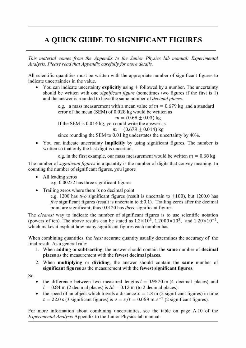
A QUICK GUIDE TO SIGNIFICANT FIGURES

This material comes from the Appendix to the Junior Physics lab manual: Experimental Analysis. Please read that Appendix carefully for more details. All scientific quantities must be written with the appropriate number of significant figures to indicate uncertainties in the value.

• You can indicate uncertainty explicitly using ± followed by a number. The uncertainty should be written with one significant figure (sometimes two figures if the first is 1) and the answer is rounded to have the same number of decimal places.

e.g. a mass measurement with a mean value of ! = 0.679!kg and a standard error of the mean (SEM) of 0.028!kg would be written as

! = (0.68± 0.03)!kg If the SEM is 0.014!kg, you could write the answer as

! = (0.679± 0.014)!kg since rounding the SEM to 0.01!kg understates the uncertainty by 40%.

• You can indicate uncertainty implicitly by using significant figures. The number is written so that only the last digit is uncertain.

e.g. in the first example, our mass measurement would be written ! = 0.68!kg The number of significant figures in a quantity is the number of digits that convey meaning. In counting the number of significant figures, you ignore

• All leading zeros e.g. 0.00252 has three significant figures

• Trailing zeros where there is no decimal point e.g. 1200 has two significant figures (result is uncertain to ±100), but 1200.0 has five significant figures (result is uncertain to ±0.1). Trailing zeros after the decimal point are significant; thus 0.0120 has three significant figures.

The clearest way to indicate the number of significant figures is to use scientific notation (powers of ten). The above results can be stated as 1.2×10!, 1.2000×10!, and 1.20×10!!, which makes it explicit how many significant figures each number has. When combining quantities, the least accurate quantity usually determines the accuracy of the final result. As a general rule:

1. When adding or subtracting, the answer should contain the same number of decimal places as the measurement with the fewest decimal places.

2. When multiplying or dividing, the answer should contain the same number of significant figures as the measurement with the fewest significant figures.

So • the difference between two measured lengths ! = 0.9570!m (4 decimal places) and

! = 0.84!m (2 decimal places) is ∆! = 0.12!m (to 2 decimal places). • the speed of an object which travels a distance ! = 1.3!m (2 significant figures) in time

! = 22.0!s (3 significant figures) is ! = !/! = 0.059!m. s!! (2 significant figures). For more information about combining uncertainties, see the table on page A.10 of the Experimental Analysis Appendix to the Junior Physics lab manual.

Combining uncertainties

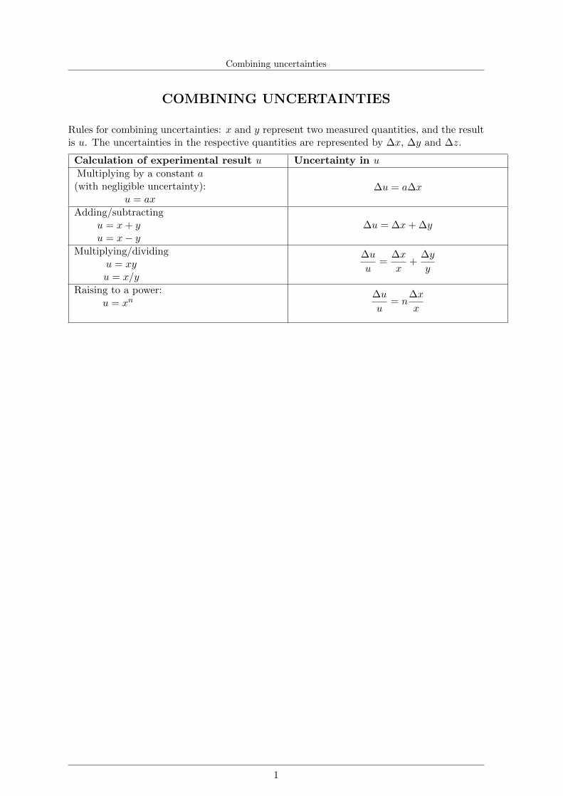
COMBINING UNCERTAINTIES

Rules for combining uncertainties: x and y represent two measured quantities, and the result

is u. The uncertainties in the respective quantities are represented by �x, �y and �z.

Calculation of experimental result u Uncertainty in u

Multiplying by a constant a

(with negligible uncertainty):

u = ax

�u = a�x

Adding/subtracting

u = x+ y

u = x� y

�u = �x+�y

Multiplying/dividing

u = xy

u = x/y

�u

u

=

�x

x

+

�y

y

Raising to a power:

u = x

n�u

u

= n

�x

x

1