C H A P T E R   7

Energy Conversion Systems – Options and Issues 7.1 Introduction  _ _ _ _ _ _ _ _ _ _ _ _ _ _ _ _ _ _ _ _ _ _ _ _ _ _ _ _ _ _ _ _ _ _7­3

7.2 Electric Power Generation  _ _ _ _ _ _ _ _ _ _ _ _ _ _ _ _ _ _ _ _ _ _ _ _ _ _7­3

7.2.1 Electricity from coproduced oil and gas operations  _ _ _ _ _ _ _ _ _ _ _ _ _ _ _7­4

7.2.2 Electricity from high­temperature EGS resources  _ _ _ _ _ _ _ _ _ _ _ _ _ _ _7­11

7.2.3 Electricity from EGS resources at supercritical conditions _ _ _ _ _ _ _ _ _ _ _7­17

7.3 Cogeneration of Electricity and Thermal Energy  _ _ _ _ _ _ _ _ _ _ _ _ _ _7­23

7.4 Plant Operational Parameters  _ _ _ _ _ _ _ _ _ _ _ _ _ _ _ _ _ _ _ _ _ _ _ _7­29

7.5 Summary and Conclusions _ _ _ _ _ _ _ _ _ _ _ _ _ _ _ _ _ _ _ _ _ _ _ _ _ _7­29

References  _ _ _ _ _ _ _ _ _ _ _ _ _ _ _ _ _ _ _ _ _ _ _ _ _ _ _ _ _ _ _ _ _ _ _ _ _7­31

7­1

Chapter 7 Energy Conversion Systems – Options and Issues

7.1 IntroductionThis section presents energy conversion (EC) systems appropriate for fluids obtained from Enhanced Geothermal Systems (EGS). A series of EC systems are given for a variety of EGS fluid conditions; temperature is the primary variable and pressure is the secondary variable.

The EC systems used here are either directly adapted from conventional hydrothermal geothermal power plants or involve appropriate modifications. In certain cases, ideas have been borrowed from the fossil­fuel power industry to cope with special conditions that may be encountered in EGS fluids. 

Several  applications  are  considered.  These  range  from  existing  “targets­of­opportunity”  associated with the coproduction of hot aqueous fluids from oil and gas wells to very hot, ultra­high­pressure geofluids produced from very deep EGS reservoirs. Although electricity generation is our principal goal,  we  also  discuss  direct­heat  applications  and  cogeneration  systems,  which  use  the  available energy in the EGS fluid for electricity generation and direct heat.

Thermodynamic analyses are carried out, sample plant­flow diagrams and layouts are presented for typical applications at both actual and hypothetical sites, and estimates are made for the capital cost of installing the power plants.

7.2 Electric Power Generation To cover a wide range of EGS fluids, we consider five cases of a geofluid at the following temperatures: 

(1) 100°C; (2) 150°C;  (3) 200°C;  (4) 250°C; (5) 400°C.

In  most  –  but  not  all  –  cases,  pressures  are  assumed  sufficient  to  maintain  the  geofluid  as  a compressed liquid (or dense, supercritical fluid) through the EGS reservoir and well system, and up 7­3

to the entry to the power­generating facility.

For each case, we have: (a) Identified the most appropriate energy conversion system. (b) Determined the expected net power per unit mass flow in kW/(kg/s). (c) Determined the mass flow required for 1, 10, and 50 MW plants. (d) Estimated the installed cost of the power plants.

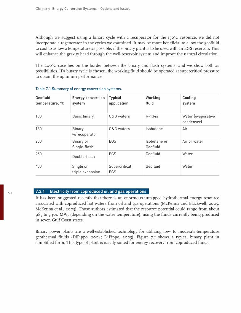
Table 7.1 summarizes the preferred energy conversion systems for the five cases. Note that the first two cases are relatively low­temperature applications, which may not apply to a high­temperature EGS system, but would apply instead to one of the “targets­of­opportunity” – namely, coproduced aqueous fluids from oil and gas operations. The last case is that of a supercritical dense fluid that could present engineering and economic challenges owing to the high pressures involved, necessitating expensive heavy­duty piping and other materials. 

Chapter 7 Energy Conversion Systems – Options and Issues

Although  we  suggest  using  a  binary  cycle  with  a  recuperator  for  the  150°C  resource,  we  did  not incorporate a regenerator in the cycles we examined. It may be more beneficial to allow the geofluid to cool to as low a temperature as possible, if the binary plant is to be used with an EGS reservoir. This will enhance the gravity head through the well­reservoir system and improve the natural circulation.

The  200°C  case  lies  on  the  border  between  the  binary  and  flash  systems,  and  we  show  both  as possibilities. If a binary cycle is chosen, the working fluid should be operated at supercritical pressure to obtain the optimum performance.

Table 7.1 Summary of energy conversion systems.

Geofluid Energy conversion  Typical  Working  Cooling temperature, °C system application fluid system

100 Basic binary O&G waters R­134a Water (evaporative

condenser)

150 Binary O&G waters Isobutane Air

w/recuperator

200 Binary or  EGS Isobutane or Air or water

Single­flash Geofluid

250 Double­flash

EGS Geofluid Water

400 Single or  Supercritical  Geofluid Water

triple expansion EGS

7.2.1 Electricity from coproduced oil and gas operations 7­4 It has been suggested  recently  that  there  is an enormous untapped hydrothermal energy  resource associated with coproduced hot waters from oil and gas operations (McKenna and Blackwell, 2005; McKenna et al., 2005). Those authors estimated that the resource potential could range from about 985 to 5,300 MWe (depending on the water temperature), using the fluids currently being produced in seven Gulf Coast states. 

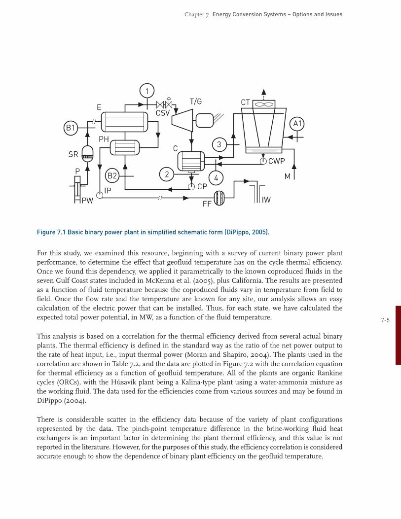
Binary  power  plants  are  a  well­established  technology  for  utilizing  low­  to  moderate­temperature geothermal  fluids  (DiPippo,  2004;  DiPippo,  2005).  Figure  7.1  shows  a  typical  binary  plant  in simplified form. This type of plant is ideally suited for energy recovery from coproduced fluids.

Chapter 7 Energy Conversion Systems – Options and Issues

T/G

C

CT

CWP

A1

3

4

1

B2 2

IP

B1

SR

PH

ECSV

P

PW

CP

FF IW

M

Figure 7.1 Basic binary power plant in simplified schematic form (DiPippo, 2005).

For  this  study, we examined  this  resource,  beginning with  a  survey of  current binary power plant performance, to determine the effect that geofluid temperature has on the cycle thermal efficiency. Once we found this dependency, we applied it parametrically to the known coproduced fluids in the seven Gulf Coast states included in McKenna et al. (2005), plus California. The results are presented as a function of fluid temperature because the coproduced fluids vary in temperature from field to field.  Once  the  flow  rate  and  the  temperature  are  known  for  any  site,  our  analysis  allows  an  easy calculation of  the electric power  that  can be  installed. Thus,  for each state, we have calculated  the expected total power potential, in MW, as a function of the fluid temperature.  7­5

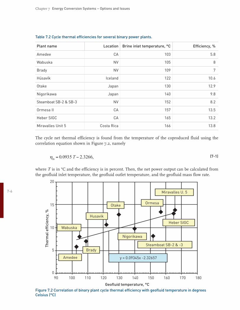
This analysis is based on a correlation for the thermal efficiency derived from several actual binary plants. The thermal efficiency is defined in the standard way as the ratio of the net power output to the rate of heat input, i.e., input thermal power (Moran and Shapiro, 2004). The plants used in the correlation are shown in Table 7.2, and the data are plotted in Figure 7.2 with the correlation equation for  thermal efficiency as a  function of geofluid  temperature. All of  the plants are organic Rankine cycles (ORCs), with the Húsavík plant being a Kalina­type plant using a water­ammonia mixture as the working fluid. The data used for the efficiencies come from various sources and may be found in DiPippo (2004).

There  is  considerable  scatter  in  the  efficiency  data  because  of  the  variety  of  plant  configurations represented  by  the  data.  The  pinch­point  temperature  difference  in  the  brine­working  fluid  heat exchangers  is  an  important  factor  in determining  the plant  thermal  efficiency, and  this  value  is not reported in the literature. However, for the purposes of this study, the efficiency correlation is considered accurate enough to show the dependence of binary plant efficiency on the geofluid temperature.

Chapter 7 Energy Conversion Systems – Options and Issues

Table 7.2 Cycle thermal efficiencies for several binary power plants.

Plant name Location Brine inlet temperature, °C Efficiency, %

Amedee CA 103 5.8

Wabuska NV 105 8

Brady NV 109 7

Húsavík Iceland 122 10.6

Otake Japan 130 12.9

Nigorikawa Japan 140 9.8

Steamboat SB­2 & SB­3 NV 152 8.2

Ormesa II CA 157 13.5

Heber SIGC CA 165 13.2

Miravalles Unit 5 Costa Rica 166 13.8

The cycle net  thermal  efficiency  is  found  from  the  temperature of  the  coproduced  fluid using  the correlation equation shown in Figure 7.2, namely

(7­1)

where T is in °C and the efficiency is in percent. Then, the net power output can be calculated from the geofluid inlet temperature, the geofluid outlet temperature, and the geofluid mass flow rate. 

7­6

900

5

10

15

20

100 110 120 130 140 150 160 170 180

Wabuska

Husavik

Amedee

Brady

Otake

y = 0.09345x -2.32657

Steamboat SB-2 & -3

Heber SIGC

Ormesa

Nigorikawa

Miravalles U. 5

Geofluid temperature, °C

Ther

mal

effic

ienc

y,%

Figure 7.2 Correlation of binary plant cycle thermal efficiency with geofluid temperature in degrees Celsius (°C) 

Chapter 7 Energy Conversion Systems – Options and Issues

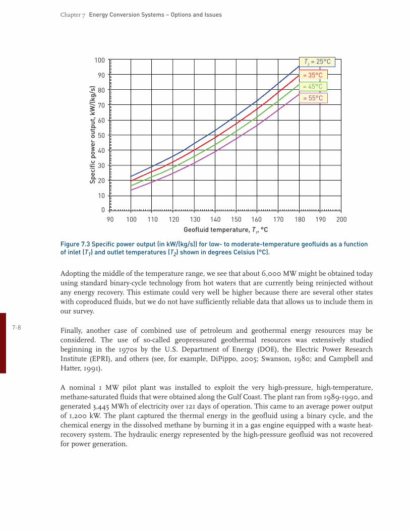
The  results  are  presented  in  the  form  shown  in  Figure  7.3,  where  T2 is  the  geofluid  temperature leaving the plant. If one knows the inlet (T1) and outlet (T2) geofluid temperatures, the power output (in kW) for a unit mass flow rate of one kg/s can be read from the graph. The total power output can then be obtained simply by multiplying this by the actual mass flow rate in kg/s. For example, a flow of 20 kg/s of a geofluid at 130°C that is discharged at 35°C can be estimated to yield a power output of 800 kW (i.e., 40 kW/(kg/s) times 20 kg/s).

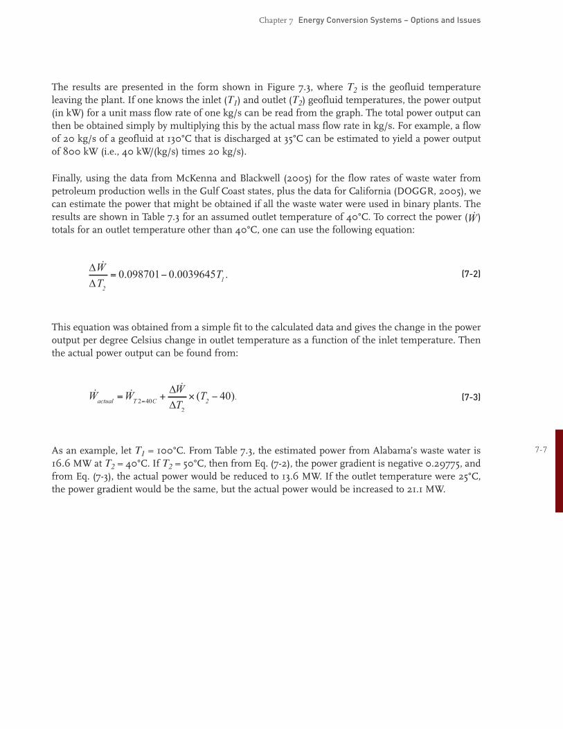
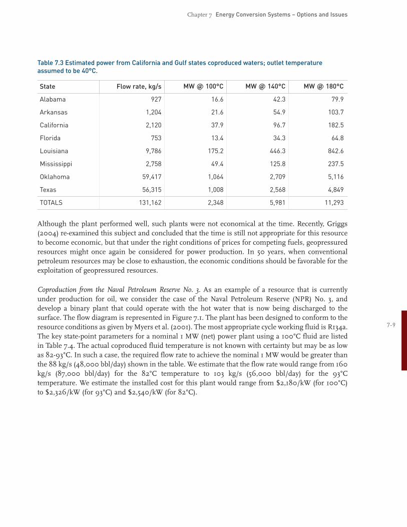
Finally, using the data from McKenna and Blackwell  (2005) for  the flow rates of waste water from petroleum production wells in the Gulf Coast states, plus the data for California (DOGGR, 2005), we can estimate the power that might be obtained if all the waste water were used in binary plants. The results are shown in Table 7.3 for an assumed outlet temperature of 40°C. To correct the power ( ) totals for an outlet temperature other than 40°C, one can use the following equation: 

(7­2)

This equation was obtained from a simple fit to the calculated data and gives the change in the power output per degree Celsius change in outlet temperature as a function of the inlet temperature. Then the actual power output can be found from:

(7­3)

As an example, let T1 = 100°C. From Table 7.3, the estimated power from Alabama’s waste water is 7­7

16.6 MW at T2 = 40°C. If T2 = 50°C, then from Eq. (7­2), the power gradient is negative 0.29775, and from Eq. (7­3), the actual power would be reduced to 13.6 MW. If the outlet temperature were 25°C, the power gradient would be the same, but the actual power would be increased to 21.1 MW.

Chapter 7 Energy Conversion Systems – Options and Issues

T2 = 25°C

= 45°C

= 35°C

= 55°C

Geofluid temperature, T1, °C

Spec

ific

pow

erou

tput

,kW

/(kg

/s)

900

10

20

30

40

50

60

70

80

90

100

100 110 120 130 140 150 160 170 180 190 200

Figure 7.3 Specific power output (in kW/(kg/s)) for low­ to moderate­temperature geofluids as a function of inlet (T1) and outlet temperatures (T2) shown in degrees Celsius (°C). 

Adopting the middle of the temperature range, we see that about 6,000 MW might be obtained today using standard binary­cycle  technology from hot waters  that are currently being reinjected without any energy recovery. This estimate could very well be higher because  there are several other states with coproduced fluids, but we do not have sufficiently reliable data that allows us to include them in our survey.

7­8 Finally,  another  case  of  combined  use  of  petroleum  and  geothermal  energy  resources  may  be considered.  The  use  of  so­called  geopressured  geothermal  resources  was  extensively  studied beginning  in  the  1970s  by  the  U.S.  Department  of  Energy  (DOE),  the  Electric  Power  Research Institute  (EPRI),  and others  (see,  for  example, DiPippo, 2005; Swanson,  1980;  and Campbell  and Hatter, 1991). 

A nominal  1  MW  pilot  plant  was  installed  to  exploit  the  very  high­pressure,  high­temperature, methane­saturated fluids that were obtained along the Gulf Coast. The plant ran from 1989­1990, and generated 3,445 MWh of electricity over 121 days of operation. This came to an average power output of  1,200 kW. The plant  captured  the  thermal  energy  in  the geofluid using  a binary  cycle,  and  the chemical energy in the dissolved methane by burning it in a gas engine equipped with a waste heat­recovery system. The hydraulic energy represented by the high­pressure geofluid was not recovered for power generation.

Chapter 7 Energy Conversion Systems – Options and Issues

Table 7.3 Estimated power from California and Gulf states coproduced waters; outlet temperature assumed to be 40°C. 

State Flow rate, kg/s MW @ 100°C MW @ 140°C MW @ 180°C

Alabama 927 16.6 42.3 79.9

Arkansas 1,204 21.6 54.9 103.7

California 2,120 37.9 96.7 182.5

Florida 753 13.4 34.3 64.8

Louisiana 9,786 175.2 446.3 842.6

Mississippi 2,758 49.4 125.8 237.5

Oklahoma 59,417 1,064 2,709 5,116

Texas 56,315 1,008 2,568 4,849

TOTALS 131,162 2,348 5,981 11,293

Although the plant performed well,  such plants were not economical at  the  time. Recently, Griggs (2004) re­examined this subject and concluded that the time is still not appropriate for this resource to become economic, but that under the right conditions of prices for competing fuels, geopressured resources  might  once  again  be  considered  for  power  production.  In  50  years,  when  conventional petroleum resources may be close to exhaustion, the economic conditions should be favorable for the exploitation of geopressured resources.

Coproduction  from  the Naval Petroleum Reserve No.  3. As  an  example  of  a  resource  that  is  currently under  production  for  oil,  we  consider  the  case  of  the  Naval  Petroleum  Reserve  (NPR)  No.  3,  and develop  a  binary  plant  that  could  operate  with  the  hot  water  that  is  now  being  discharged  to  the surface. The flow diagram is represented in Figure 7.1. The plant has been designed to conform to the resource conditions as given by Myers et al. (2001). The most appropriate cycle working fluid is R134a. 7­9

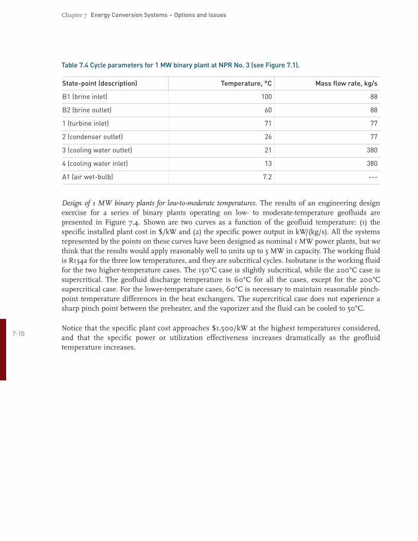
The key state­point parameters for a nominal 1 MW (net) power plant using a 100°C fluid are listed in Table 7.4. The actual coproduced fluid temperature is not known with certainty but may be as low as 82­93°C. In such a case, the required flow rate to achieve the nominal 1 MW would be greater than the 88 kg/s (48,000 bbl/day) shown in the table. We estimate that the flow rate would range from 160 kg/s  (87,000  bbl/day)  for  the  82°C  temperature  to  103  kg/s  (56,000  bbl/day)  for  the  93°C temperature. We estimate the installed cost for this plant would range from $2,180/kW (for 100°C) to $2,326/kW (for 93°C) and $2,540/kW (for 82°C).

­­­

Chapter 7 Energy Conversion Systems – Options and Issues

Table 7.4 Cycle parameters for 1 MW binary plant at NPR No. 3 (see Figure 7.1).

State­point (description) Temperature, °C Mass flow rate, kg/s

B1 (brine inlet) 100 88

B2 (brine outlet) 60 88

1 (turbine inlet) 71 77

2 (condenser outlet) 26 77

3 (cooling water outlet) 21 380

4 (cooling water inlet) 13 380

A1 (air wet­bulb) 7.2

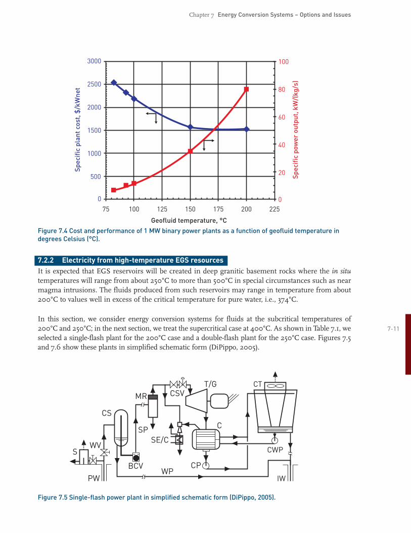
Design of  1 MW binary plants  for  low­to­moderate  temperatures. The results of an engineering design exercise  for  a  series  of  binary  plants  operating  on  low­  to  moderate­temperature  geofluids  are presented  in  Figure  7.4.  Shown  are  two  curves  as  a  function  of  the  geofluid  temperature:  (1)  the specific installed plant cost in $/kW and (2) the specific power output in kW/(kg/s). All the systems represented by the points on these curves have been designed as nominal 1 MW power plants, but we think that the results would apply reasonably well to units up to 5 MW in capacity. The working fluid is R134a for the three low temperatures, and they are subcritical cycles. Isobutane is the working fluid for the two higher­temperature cases. The 150°C case is slightly subcritical, while the 200°C case is supercritical.  The  geofluid  discharge  temperature  is  60°C  for  all  the  cases,  except  for  the  200°C supercritical case. For the lower­temperature cases, 60°C is necessary to maintain reasonable pinch­point  temperature differences  in  the heat exchangers. The supercritical case does not experience a sharp pinch point between the preheater, and the vaporizer and the fluid can be cooled to 50°C. 

Notice that the specific plant cost approaches $1,500/kW at the highest temperatures considered, 7­10 and  that  the  specific  power  or  utilization  effectiveness  increases  dramatically  as  the  geofluid

temperature increases.

Chapter 7 Energy Conversion Systems – Options and Issues

Geofluid temperature, °C

Spec

ific

plan

tcos

t,$

/kW

net

Spec

ific

pow

erou

tput

,kW

/(kg

/s)

75 100 125 150 175 200 225

0 0

20

40

60

80

100

500

1000

1500

2000

2500

3000

Figure 7.4 Cost and performance of 1 MW binary power plants as a function of geofluid temperature in degrees Celsius (°C).

7.2.2 Electricity from high­temperature EGS resources

It is expected that EGS reservoirs will be created in deep granitic basement rocks where the in situ temperatures will range from about 250°C to more than 500°C in special circumstances such as near magma intrusions. The fluids produced from such reservoirs may range in temperature from about 200°C to values well in excess of the critical temperature for pure water, i.e., 374°C.

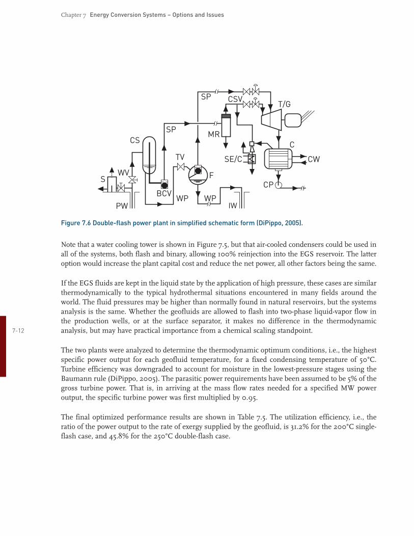
In  this  section,  we  consider  energy  conversion  systems  for  fluids  at  the  subcritical  temperatures  of 200°C and 250°C; in the next section, we treat the supercritical case at 400°C. As shown in Table 7.1, we 7­11

selected a single­flash plant for the 200°C case and a double­flash plant for the 250°C case. Figures 7.5 and 7.6 show these plants in simplified schematic form (DiPippo, 2005).

CT

CWP

IW

T/G

C

MR

CS

WVS

CPWP

SE/C

CSV

SP

PW

BCV

Figure 7.5 Single­flash power plant in simplified schematic form (DiPippo, 2005).

Chapter 7 Energy Conversion Systems – Options and Issues

IW

CCSSP

WVS

CP

SE/C

MR

T/GCSV

CW

SP

TV

F

PWWP WPBCV

Figure 7.6 Double­flash power plant in simplified schematic form (DiPippo, 2005).

Note that a water cooling tower is shown in Figure 7.5, but that air­cooled condensers could be used in all of the systems, both flash and binary, allowing 100% reinjection into the EGS reservoir. The latter option would increase the plant capital cost and reduce the net power, all other factors being the same.

If the EGS fluids are kept in the liquid state by the application of high pressure, these cases are similar thermodynamically  to  the  typical  hydrothermal  situations  encountered  in  many  fields  around  the world. The fluid pressures may be higher than normally found in natural reservoirs, but the systems analysis is the same. Whether the geofluids are allowed to flash into two­phase liquid­vapor flow in the  production  wells,  or  at  the  surface  separator, it  makes  no  difference  in  the  thermodynamic

7­12 analysis, but may have practical importance from a chemical scaling standpoint.

The two plants were analyzed to determine the thermodynamic optimum conditions, i.e., the highest specific  power  output  for  each  geofluid  temperature,  for  a  fixed  condensing  temperature  of  50°C. Turbine efficiency was downgraded to account for moisture in the lowest­pressure stages using the Baumann rule (DiPippo, 2005). The parasitic power requirements have been assumed to be 5% of the gross  turbine power. That  is,  in  arriving at  the mass  flow  rates needed  for  a  specified MW power output, the specific turbine power was first multiplied by 0.95. 

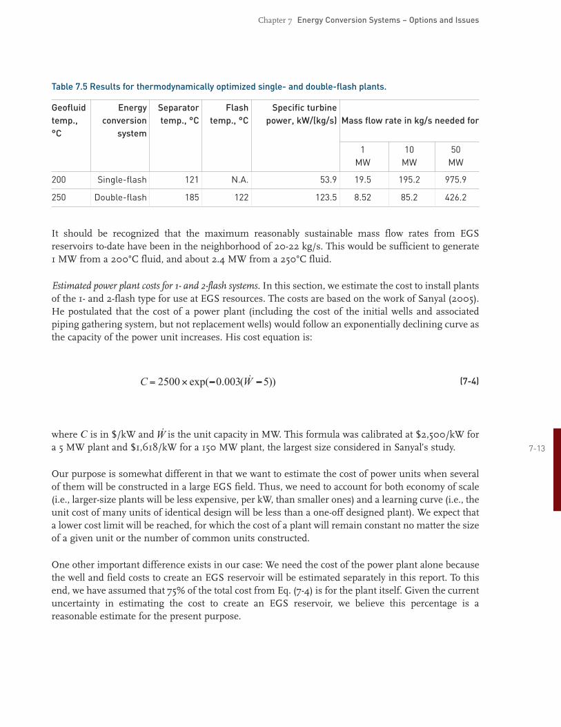
The final optimized performance results are shown in Table 7.5. The utilization efficiency,  i.e.,  the ratio of the power output to the rate of exergy supplied by the geofluid, is 31.2% for the 200°C single­flash case, and 45.8% for the 250°C double­flash case.

200

250

Chapter 7 Energy Conversion Systems – Options and Issues

Table 7.5 Results for thermodynamically optimized single­ and double­flash plants.

Geofluid

°C

Flash Specific turbine

1

MW

10

MW

50

MW

temp., Energy

conversion

system

Separator

temp., °C temp., °C power, kW/(kg/s) Mass flow rate in kg/s needed for

Single­flash 121 N.A. 53.9 19.5 195.2 975.9

Double­flash 185 122 123.5 8.52 85.2 426.2

It  should  be  recognized  that  the  maximum  reasonably  sustainable  mass  flow  rates  from  EGS reservoirs to­date have been in the neighborhood of 20­22 kg/s. This would be sufficient to generate 1 MW from a 200°C fluid, and about 2.4 MW from a 250°C fluid.

Estimated power plant costs for 1­ and 2­flash systems. In this section, we estimate the cost to install plants of the 1­ and 2­flash type for use at EGS resources. The costs are based on the work of Sanyal (2005). He postulated  that  the cost of  a power plant  (including  the cost of  the  initial wells  and associated piping gathering system, but not replacement wells) would follow an exponentially declining curve as the capacity of the power unit increases. His cost equation is:

(7­4)

where C is in $/kW and  is the unit capacity in MW. This formula was calibrated at $2,500/kW for a 5 MW plant and $1,618/kW for a 150 MW plant, the largest size considered in Sanyal’s study. 7­13

Our purpose is somewhat different in that we want to estimate the cost of power units when several of them will be constructed in a large EGS field. Thus, we need to account for both economy of scale (i.e., larger­size plants will be less expensive, per kW, than smaller ones) and a learning curve (i.e., the unit cost of many units of identical design will be less than a one­off designed plant). We expect that a lower cost limit will be reached, for which the cost of a plant will remain constant no matter the size of a given unit or the number of common units constructed.

One other important difference exists in our case: We need the cost of the power plant alone because the well and field costs to create an EGS reservoir will be estimated separately in this report. To this end, we have assumed that 75% of the total cost from Eq. (7­4) is for the plant itself. Given the current uncertainty  in  estimating  the  cost  to  create  an  EGS  reservoir, we  believe  this  percentage  is  a reasonable estimate for the present purpose.

Chapter 7 Energy Conversion Systems – Options and Issues

Thus, we adapted Sanyal’s equation to suit the present needs and used the following formulation:

(7­5)

or

(7­6)

This  equation gives $1,875/kW for  the plant  cost,  exclusive of  initial wells,  for  a  5 MW plant;  and $1,213/kW for a 150 MW plant (the same as Sanyal’s equation), but includes an asymptotic plant cost of  $750/kW  for  large  units  or  for  very  large  numbers  of  common  units.  This  limit  cost  is  our judgment, based on experience with actual, recently constructed plants.

We  want  to  show  how  the  temperature  of  the  EGS  resource  affects  the  cost  of  the  plant.  For  this purpose, we calculated the exergy of the geofluid coming from the EGS reservoir at any temperature. This value was multiplied by the utilization efficiency for optimized 1­ and 2­flash plants to obtain the power output that should be attainable from the geofluid. This power was then used in Eq. (7­6) to obtain the estimated cost of the power unit. 

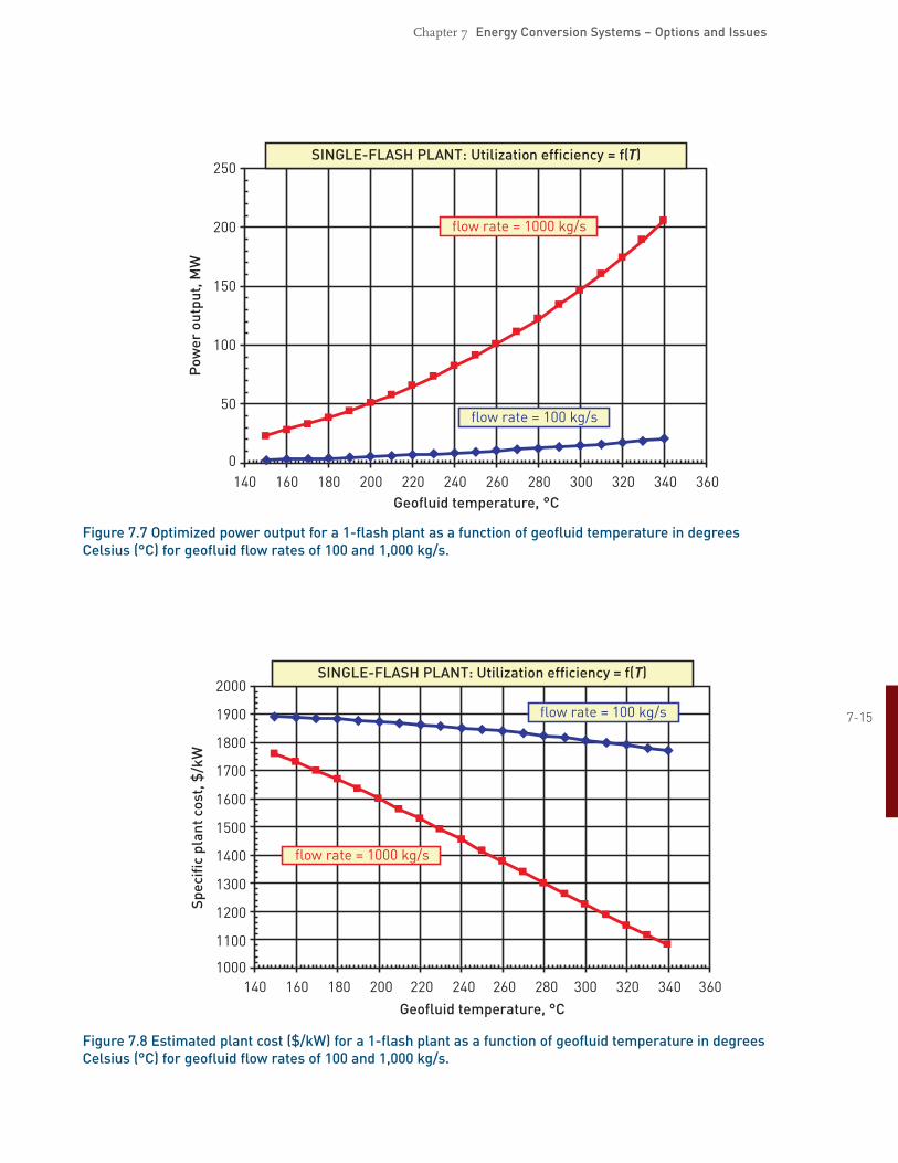
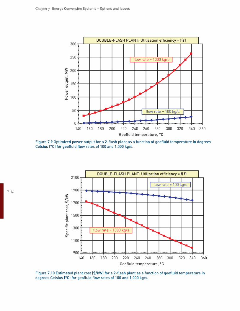
The results are shown in Figures 7.7 to 7.10, which cover the range of temperatures expected from EGS systems. Figures 7.7 and 7.9 show the optimized power output, and Figures 7.8 and 7.10 show the plant costs, for 1­and 2­flash plants, respectively. The dramatic reductions in cost per kW for the

7­14 higher flow rates are evident, which, of course, mean higher power ratings. 

A nominal  50  MW  plant  can  be  obtained  from  1,000  kg/s  at  200°C  using  a  1­flash  plant  at  an estimated  cost of $1,600/kW. The  same power output  can be obtained  from a 2­flash plant using 1,000 kg/s at 180°C for $1,650/kW.

Chapter 7 Energy Conversion Systems – Options and Issues

Geofluid temperature, °C

Pow

erou

tput

,MW

140 160 180 200 220 240 260 280 300 320 340 3600

50

100

150

200

250SINGLE-FLASH PLANT: Utilization efficiency = f(T)

flow rate = 1000 kg/s

flow rate = 100 kg/s

Figure 7.7 Optimized power output for a 1­flash plant as a function of geofluid temperature in degrees Celsius (°C) for geofluid flow rates of 100 and 1,000 kg/s.

7­15

Geofluid temperature, °C

Spec

ific

plan

tcos

t,$

/kW

140 160 180 200 220 240 260 280 300 320 340 3601000

1100

1200

1300

1400

1500

1600

1700

1800

1900

2000SINGLE-FLASH PLANT: Utilization efficiency = f(T)

flow rate = 1000 kg/s

flow rate = 100 kg/s

Figure 7.8 Estimated plant cost ($/kW) for a 1­flash plant as a function of geofluid temperature in degrees Celsius (°C) for geofluid flow rates of 100 and 1,000 kg/s.

Chapter 7 Energy Conversion Systems – Options and Issues

Geofluid temperature, °C

Pow

erou

tput

,MW

140 160 180 200 220 240 260 280 300 320 340 360 10

50

100

150

200

250

300DOUBLE-FLASH PLANT: Utilization efficiency = f(T)

flow rate = 1000 kg/s

flow rate = 100 kg/s

Figure 7.9 Optimized power output for a 2­flash plant as a function of geofluid temperature in degrees Celsius (°C) for geofluid flow rates of 100 and 1,000 kg/s.

7­16

Geofluid temperature, °C

Spec

ific

plan

tcos

t,$

/kW

140 160 180 200 220 240 260 280 300 320 340 360 1900

1100

1300

1500

1700

1900

2100DOUBLE-FLASH PLANT: Utilization efficiency = f(T)

flow rate = 1000 kg/s

flow rate = 100 kg/s

Figure 7.10 Estimated plant cost ($/kW) for a 2­flash plant as a function of geofluid temperature in degrees Celsius (°C) for geofluid flow rates of 100 and 1,000 kg/s.

Chapter 7 Energy Conversion Systems – Options and Issues

7.2.3 Electricity from EGS resources at supercritical conditions

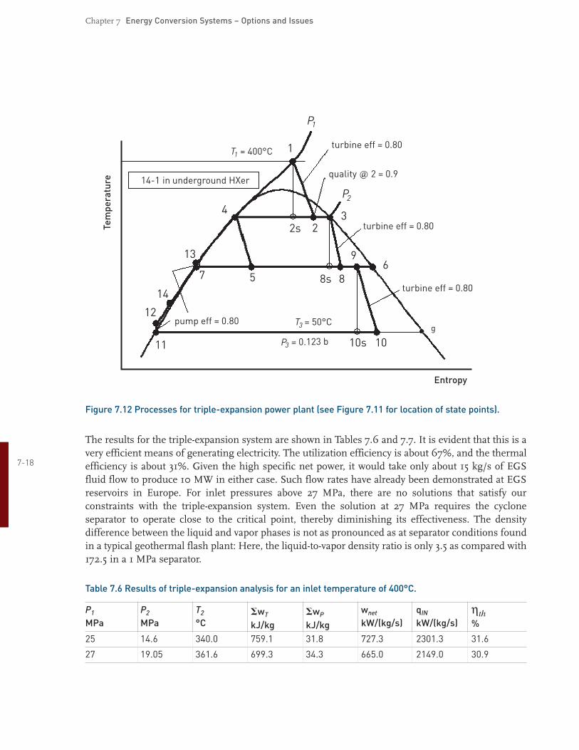
A novel energy conversion system was developed to handle the cases when the EGS geofluid arrives at the plant at supercritical conditions, i.e., at a temperature greater than 374°C and a pressure greater than 22 MPa. For all situations studied, the temperature was taken as constant at 400°C. The plant is called the “triple­expansion” system; it is shown in simplified schematic form in Figure 7.11, and the thermodynamic processes are shown in the temperature­entropy diagram in Figure 7.12.

The  triple­expansion  system  is  a  variation  on  the  conventional  double­flash  system,  with  the addition of a “topping” dense­fluid, back­pressure turbine, shown as item SPT in Figure 7.11. The turbine is designed to handle the very high pressures postulated for the EGS geofluid, in much the same manner as a “superpressure” turbine in a fossil­fueled supercritical double­reheat power plant (El Wakil, 1984). However,  in this case, we impose a limit on the steam quality  leaving the SPT to avoid excessive moisture and blade erosion.

The analysis was based on the following assumptions:

• Geofluid inlet temperature, T1 = 400°C. • Geofluid pressure, P1 > 22 MPa. • Condenser temperature and pressure: T10 = 50°C and P10 = 0.123 bar = 0.0123 MPa. • All turbine and pump isentropic efficiencies are 80%. • Steam quality at SPT exit, state 2 = 0.90. • HPT­ and LPT­turbine outlet steam qualities (states 8 and 10) are unconstrained.

To determine the “optimum” performance, we selected the temperature at the outlet of the flash vessel (state­point 5) as the average between the temperature at the SPT outlet (state 2) and the condenser (state 10), in accordance with the approximate rule­of­thumb for optimizing geothermal double­flash plants  (DiPippo,  2005).  No claim  is  made,  however, that  this  will  yield  the  true  optimum  triple­expansion design, but it should not be far off.

7­17

SPT

BCVIW

C

WVS

LPT

HPT

HPP

CW

LPPTV

CS

F

PW

10

11

5

4

2

7

1

12

98

3

6

1413

Figure 7.11 Triple­expansion power plant for supercritical EGS fluids.

Chapter 7 Energy Conversion Systems – Options and Issues

T = 400°C

14-1 in underground HXer

11

T = 50°C3

P = 0.123 b3

69

32

4

13

14

12

11

7 5 8s 8

g

2s

10s 10

P2

Tem

pera

ture

turbine eff = 0.80

quality @ 2 = 0.9

turbine eff = 0.80

turbine eff = 0.80

Entropy

pump eff = 0.80

P1

Figure 7.12 Processes for triple­expansion power plant (see Figure 7.11 for location of state points).

The results for the triple­expansion system are shown in Tables 7.6 and 7.7. It is evident that this is a very efficient means of generating electricity. The utilization efficiency is about 67%, and the thermal

7­18 efficiency is about 31%. Given the high specific net power, it would take only about 15 kg/s of EGS fluid flow to produce 10 MW in either case. Such flow rates have already been demonstrated at EGS reservoirs  in  Europe.  For  inlet  pressures  above  27  MPa,  there  are  no  solutions  that  satisfy  our constraints  with  the  triple­expansion  system.  Even  the  solution  at  27  MPa  requires  the  cyclone separator  to  operate  close  to  the  critical  point,  thereby  diminishing  its  effectiveness.  The  density difference between the liquid and vapor phases is not as pronounced as at separator conditions found in a typical geothermal flash plant: Here, the liquid­to­vapor density ratio is only 3.5 as compared with 172.5 in a 1 MPa separator.

Table 7.6 Results of triple­expansion analysis for an inlet temperature of 400°C.

P1 P2 T2 wnet qIN�wT �wP ηth MPa MPa °C kW/(kg/s) kW/(kg/s) %kJ/kg kJ/kg

25 14.6 340.0 759.1 31.8 727.3 2301.3 31.6

27 19.05 361.6 699.3 34.3 665.0 2149.0 30.9

Chapter 7 Energy Conversion Systems – Options and Issues

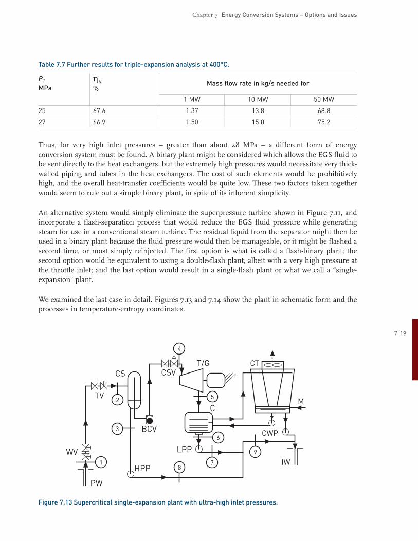
Table 7.7 Further results for triple­expansion analysis at 400°C.

P1 MPa

ηu %

Mass flow rate in kg/s needed for

1 MW 10 MW 50 MW

25 67.6 1.37 13.8 68.8

27 66.9 1.50 15.0 75.2

Thus,  for  very  high  inlet  pressures  –  greater  than  about  28  MPa  –  a  different  form  of  energy conversion system must be found. A binary plant might be considered which allows the EGS fluid to be sent directly to the heat exchangers, but the extremely high pressures would necessitate very thick­walled piping and  tubes  in  the heat exchangers. The cost of  such elements would be prohibitively high, and the overall heat­transfer coefficients would be quite low. These two factors taken together would seem to rule out a simple binary plant, in spite of its inherent simplicity.

An alternative system would simply eliminate the superpressure turbine shown in Figure 7.11, and incorporate  a  flash­separation  process  that  would  reduce  the  EGS  fluid  pressure  while  generating steam for use in a conventional steam turbine. The residual liquid from the separator might then be used in a binary plant because the fluid pressure would then be manageable, or it might be flashed a second  time,  or most  simply  reinjected. The  first  option  is what  is  called  a  flash­binary plant;  the second option would be equivalent to using a double­flash plant, albeit with a very high pressure at the  throttle  inlet; and  the  last option would result  in a single­flash plant or what we call a “single­expansion” plant.

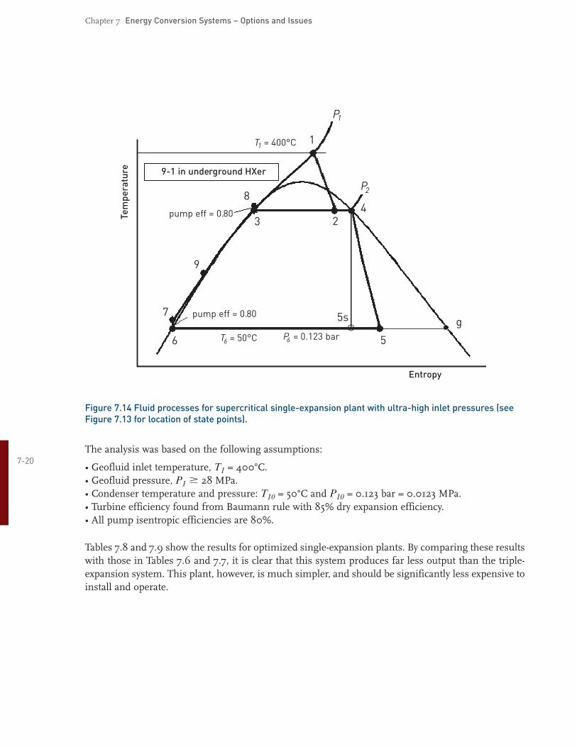
We examined the last case in detail. Figures 7.13 and 7.14 show the plant in schematic form and the processes in temperature­entropy coordinates. 

7­19

71

2

9

63

5

CT

M

CWP

IW

T/G

C

LPP

CSVCS

TV

BCV

HPP

PW

WV

8

4

Figure 7.13 Supercritical single­expansion plant with ultra­high inlet pressures.

Chapter 7 Energy Conversion Systems – Options and Issues

T = 400°C

9-1 in underground HXer

11

T = 50°C6 P = 0.123 bar6

P

6

9

3 24

7

5

5s

8

g

1Te

mpe

ratu

re

Entropy

pump eff = 0.80

pump eff = 0.80

P2

Figure 7.14 Fluid processes for supercritical single­expansion plant with ultra­high inlet pressures (see Figure 7.13 for location of state points).

The analysis was based on the following assumptions: 7­20

• Geofluid inlet temperature, T1 = 400°C. • Geofluid pressure, P1 � 28 MPa. • Condenser temperature and pressure: T10 = 50°C and P10 = 0.123 bar = 0.0123 MPa. • Turbine efficiency found from Baumann rule with 85% dry expansion efficiency. • All pump isentropic efficiencies are 80%.

Tables 7.8 and 7.9 show the results for optimized single­expansion plants. By comparing these results with those in Tables 7.6 and 7.7, it is clear that this system produces far less output than the triple­expansion system. This plant, however, is much simpler, and should be significantly less expensive to install and operate.

Chapter 7 Energy Conversion Systems – Options and Issues

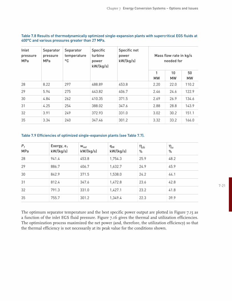
Table 7.8 Results of thermodynamically optimized single­expansion plants with supercritical EGS fluids at 400°C and various pressures greater than 27 MPa.

°C

Specific turbine 

Specific net

1

MW

10

MW

50

MW

Inlet pressure

MPa

Separator

pressure

MPa

Separator

temperature

power kW/(kg/s)

power kW/(kg/s)

Mass flow rate in kg/s needed for

28 8.22 297 488.89 453.8 2.20 22.0 110.2

29 5.94 275 443.82 406.7 2.46 24.6 122.9

30 4.84 262 410.35 371.5 2.69 26.9 134.6

31 4.25 254 388.02 347.6 2.88 28.8 143.9

32 3.91 249 372.93 331.0 3.02 30.2 151.1

35 3.34 240 347.46 301.2 3.32 33.2 166.0

Table 7.9 Efficiencies of optimized single­expansion plants (see Table 7.7).

P1 Exergy, e1 wnet qIN ηth ηu MPa kW/(kg/s) kW/(kg/s) kW/(kg/s) % %

28 941.4 453.8 1,754.3 25.9 48.2

29 886.7 406.7 1,632.7 24.9 45.9

30 842.9 371.5 1,538.0 24.2 44.1

31 812.4 347.6 1,472.8 23.6 42.8 7­21

32 791.3 331.0 1,427.1 23.2 41.8

35 755.7 301.2 1,349.4 22.3 39.9

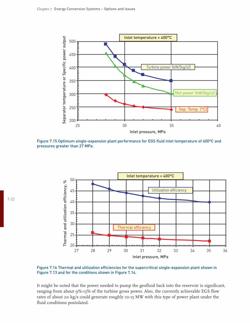
The optimum separator temperature and the best specific power output are plotted in Figure 7.15 as a function of the inlet EGS fluid pressure. Figure 7.16 gives the thermal and utilization efficiencies. The optimization process maximized the net power (and, therefore, the utilization efficiency) so that the thermal efficiency is not necessarily at its peak value for the conditions shown.

Chapter 7 Energy Conversion Systems – Options and Issues

Inlet pressure, MPa

Sepa

rato

rte

mpe

ratu

reor

Spec

ific

pow

erou

tput

25 30 35 40 1200

250

300

350

400

450

500Inlet temperature = 400°C

Sep. Temp. (°C)

Net power (kW/(kg/s))

Turbine power (kW/(kg/s))

Figure 7.15 Optimum single­expansion plant performance for EGS fluid inlet temperature of 400°C and pressures greater than 27 MPa.

7­22

Inlet pressure, MPa

Ther

mal

and

utili

zati

onef

ficie

ncy,

%

27 28 29 30 31 32 33 34 35 36 120

25

30

35

40

45

50Inlet temperature = 400°C

Thermal efficiency

Utilization efficiency

Figure 7.16 Thermal and utilization efficiencies for the supercritical single­expansion plant shown in Figure 7.13 and for the conditions shown in Figure 7.14.

It might be noted that the power needed to pump the geofluid back into the reservoir is significant, ranging from about 9%­13% of the turbine gross power. Also, the currently achievable EGS flow rates of about 20 kg/s could generate roughly 10­15 MW with this type of power plant under the fluid conditions postulated.

Chapter 7 Energy Conversion Systems – Options and Issues

Thus,  for  supercritical  geofluids  from EGS  reservoirs, we  conclude  that  for  those  cases where  the geofluid is supplied to the plant at a temperature of 400°C, and at pressures greater than 22 MPa but less  than 28 MPa,  the preferred energy conversion system is a relatively complex,  triple­expansion system. Cycle thermal efficiencies of about 31% and utilization efficiencies of 67% can be expected.

For  cases  where  the  geofluid  is  supplied  to  the  plant  at  a  temperature  of  400°C  and  at  pressures greater  than  28  MPa,  the  preferred  energy  conversion  system  is  a  single­expansion  system.  Cycle thermal efficiencies of about 24% and utilization efficiencies of 40%­45% can be expected.

The  analysis  presented  here  does  not  account  for  pressure  losses  through  any  piping  or  heat exchangers,  including  the  manufactured  one  in  the  underground  reservoir.  Once  the  reservoir performance has been determined in the field, this can easily be taken into account by adjusting the required pump work. 

We are  left  to  speculate what geofluid pressures are  reasonable  for  the EGS environment. For  the simpler  energy  conversion  system  (i.e.,  the  single­expansion  cycle),  the  higher  the  pressure,  the poorer the performance of the power cycle. The best performance occurs at pressures that may be too low to provide sufficient throughput of geofluid. For the more complex, triple­expansion system, it is not known whether the very high pressures postulated, requiring expensive thick­walled piping and vessels, may render this system uneconomic. Finally, at this stage of our understanding, we have no idea what geofluid flow rates will accompany any particular geofluid pressure because of  the great uncertainty regarding the flow in the manufactured underground reservoir. More fieldwork is needed to shed light on this issue. 

7.3 Cogeneration of Electricity and Thermal Energy

7­23One of the possible uses of EGS­produced fluids is to provide both electricity and heat to residential, commercial,  industrial,  or  institutional  users.  In  this  section,  we  consider  the  case  of  the  MIT cogeneration system (MIT­COGEN) as a typical application. 

Our tasks for the cogeneration case are: (a) Identify the most appropriate energy conversion system using hot geofluid from an EGS

resource that will supply all the required energy flows of the current system, i.e., electricity, heating, and air conditioning.

(b) Calculate the required flow rate of the geofluid.

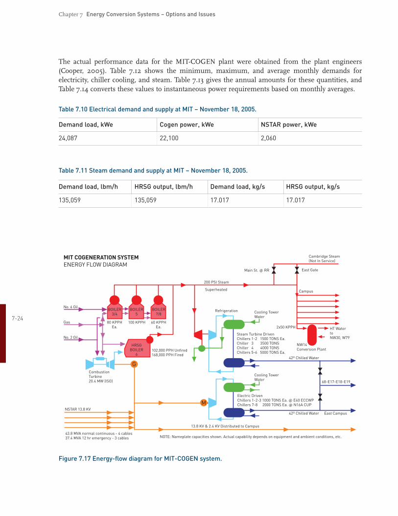
MIT­COGEN  employs  a  gas  turbine  with  a  waste  heat­recovery  steam  generator  (HRSG)  to  meet nearly all of the electrical and heating/cooling needs of the campus – Tables 7.10 and 7.11 give HRSG a snapshot of  the energy outputs  for November 18, 2005. Also, on November 18, 2005,  the steam generated from the HRSG was at 1.46 MPa and 227°C, with 30°C of superheat. Figure 7.17 shows the energy flow diagram for the plant (Cooper, 2005), and Figure 7.18 is a highly simplified flow diagram for the main components of the system. It is important to note that the chiller plant is powered mainly by steam turbines that drive the compressors, the steam being raised in the HRSG of the gas turbine plant. Two of the chillers have electric motor­driven compressors.

Chapter 7 Energy Conversion Systems – Options and Issues

The  actual  performance  data  for  the  MIT­COGEN  plant  were  obtained  from  the  plant  engineers (Cooper,  2005).  Table  7.12  shows  the  minimum,  maximum,  and  average  monthly  demands  for electricity, chiller cooling, and steam. Table 7.13 gives the annual amounts for these quantities, and Table 7.14 converts these values to instantaneous power requirements based on monthly averages.

Table 7.10 Electrical demand and supply at MIT – November 18, 2005.

Demand load, kWe Cogen power, kWe NSTAR power, kWe

24,087 22,100 2,060

Table 7.11 Steam demand and supply at MIT – November 18, 2005.

Demand load, lbm/h HRSG output, lbm/h Demand load, kg/s HRSG output, kg/s

135,059 135,059 17.017 17.017

7­24

G

M

CombustionTurbine20.4 MW (ISO)

NSTAR 13.8 KV

43.8 MVA normal continuous - 4 cables37.4 MVA 12 hr emergency - 3 cables

68-E17-E18-E19

East Campus42º Chilled Water

NOTE: Nameplate capacities shown. Actual capability depends on equipment and ambient conditions, etc.

13.8 KV & 2.4 KV Distributed to Campus

42º Chilled Water

Cooling TowerWater

Cooling TowerWater

Refrigeration

Superheated

200 PSI Steam

Main St. @ RR East Gate

Campus

Cambridge Steam(Not In Service)

NW14Conversion Plant

HT WatertoNW30, W79

2x50 KPPH

Steam Turbine DrivenChillers 1-2 1500 TONS Ea.Chiller 3 3500 TONSChiller 4 4000 TONSChillers 5-6 5000 TONS Ea.

Electric DrivenChillers 1-2-3 1000 TONS Ea. @ E40 ECCWPChillers 7-8 2000 TONS Ea. @ N16A CUP

BOILER3/4

80 KPPHEa.

No. 6 Oil

MIT COGENERATION SYSTEMENERGY FLOW DIAGRAM

No. 2 Oil

Gas 60 KPPHEa.

102,000 PPH Unfired168,000 PPH Fired

100 KPPH

BOILER5

HRSGBOILER

6

BOILER7/8

Figure 7.17 Energy­flow diagram for MIT­COGEN system.

Chapter 7 Energy Conversion Systems – Options and Issues

MITHeatingLoad

FUEL

CC

AIR

FUEL

HRSGBoiler No. 6

To Stack

PPP

EC

B

SH

Vapor-compressionChillers

MITCoolingLoad

TCG

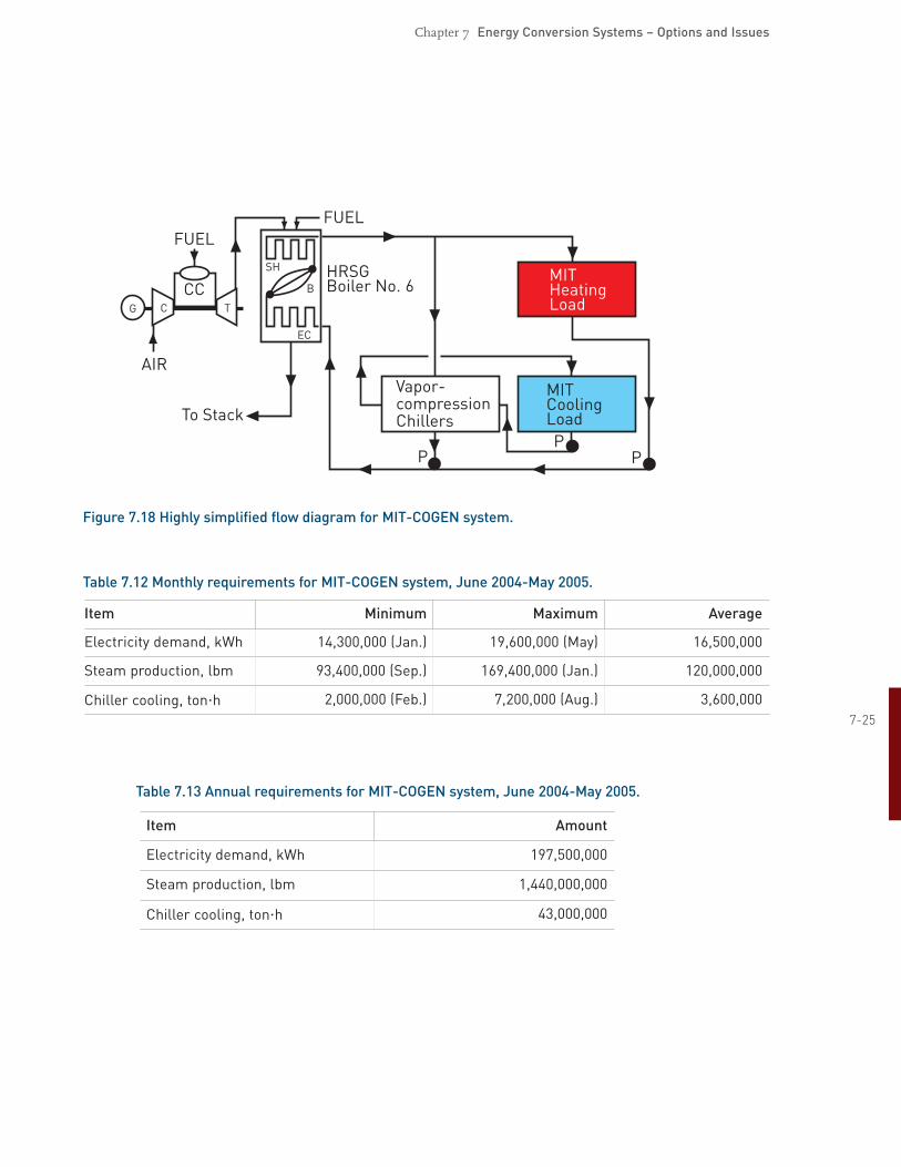
Figure 7.18 Highly simplified flow diagram for MIT­COGEN system.

Table 7.12 Monthly requirements for MIT­COGEN system, June 2004­May 2005.

Item Minimum Maximum Average

Electricity demand, kWh 14,300,000 (Jan.) 19,600,000 (May) 16,500,000

Steam production, lbm 93,400,000 (Sep.) 169,400,000 (Jan.) 120,000,000

Chiller cooling, ton·h 2,000,000 (Feb.) 7,200,000 (Aug.) 3,600,000 7­25

Table 7.13 Annual requirements for MIT­COGEN system, June 2004­May 2005.

Item Amount

Electricity demand, kWh 197,500,000

Steam production, lbm 1,440,000,000

Chiller cooling, ton·h 43,000,000

Chapter 7 Energy Conversion Systems – Options and Issues

Table 7.14 Average power needs for MIT­COGEN system, June 2004­May 2005.

Item Amount

Electricity demand, kW 22,900

Steam production, lbm/h 167,000

Steam production, kg/s 21

Chiller cooling, ton 5,000

Chiller cooling, Btu/h 60,000,000

Chiller cooling, kWth 17,500

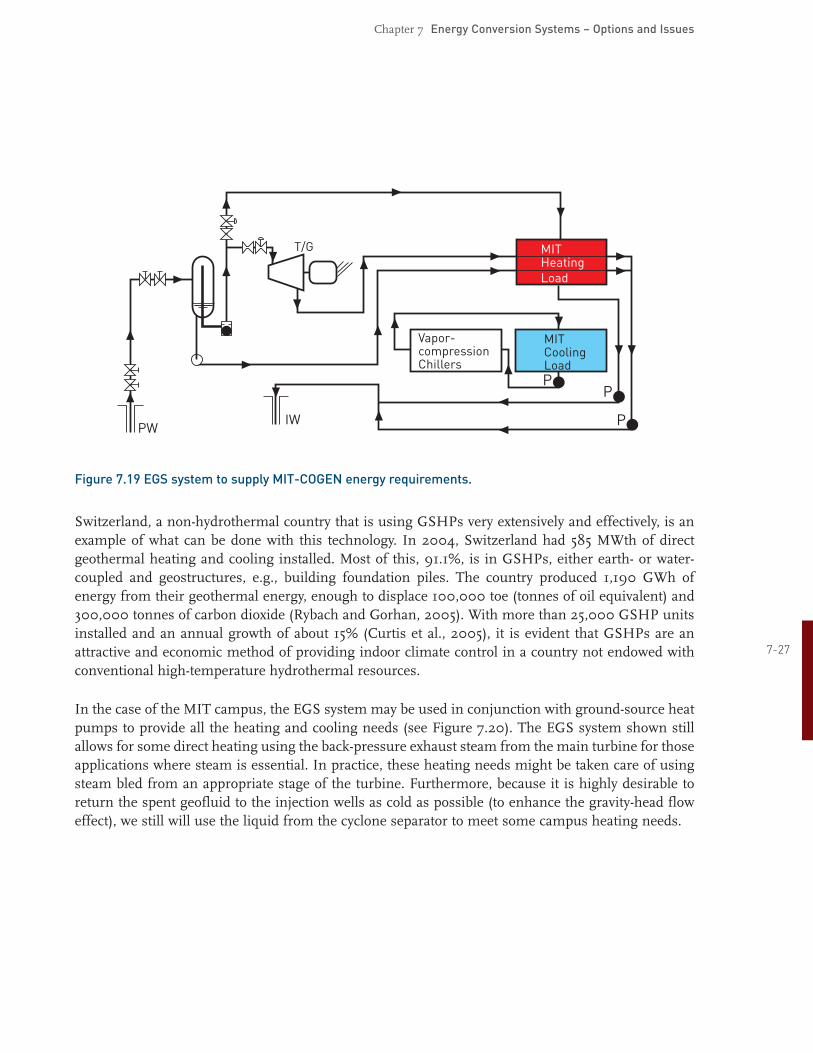
Figure 7.19 is a flow diagram in which an EGS wellfield replaces the fossil energy input to the existing MIT­COGEN plant and supplies all of the current energy requirements. 

The current gas turbine generator set is rated at 20 MW but usually puts out more than that, typically 22  MW; the  remainder  of  the  electrical  load  must  be  supplied  by  the  local  utility.  The  power requirements will have to be produced by a new steam turbine driven by EGS­produced steam. We have selected a single­flash system with a back­pressure steam turbine. The exhaust steam from the turbine will be condensed against part of the heating load, thereby providing a portion of the total load for the moderate­ to lower­temperature applications. The separated liquid from the cyclone separators may also be used to supply some of the needs of the heating system. 

If the EGS system were to replicate the existing chiller plant, a side stream of the separated steam generated  in  the  cyclone  separator  would  be  needed  to  drive  the  steam  turbine­compressor  sets. However, we think  it  is more practical  for  the EGS system to provide sufficient electricity  from its steam turbine­generator to supply electric motors to power the chiller compressors.

7­26

Another innovation that fits the new EGS system is to retrofit the campus to meet the heating and space  cooling  needs  with  ground­source  heat  pumps  (GSHP).  In  the  long­range  view  of  this assessment, it will be beneficial to use GSHPs for space conditioning and to use electricity to drive the compressors.

Chapter 7 Energy Conversion Systems – Options and Issues

PWIW

MITHeatingLoad

T/G

Vapor-compressionChillers

MITCoolingLoad

P

PP

Figure 7.19 EGS system to supply MIT­COGEN energy requirements.

Switzerland, a non­hydrothermal country that is using GSHPs very extensively and effectively, is an example of what  can be done with  this  technology.  In 2004, Switzerland had  585 MWth of direct geothermal heating and cooling installed. Most of  this, 91.1%, is  in GSHPs, either earth­ or water­coupled  and  geostructures,  e.g.,  building  foundation  piles.  The  country  produced  1,190  GWh  of energy from their geothermal energy, enough to displace 100,000 toe (tonnes of oil equivalent) and 300,000 tonnes of carbon dioxide (Rybach and Gorhan, 2005). With more than 25,000 GSHP units installed and an annual growth of about 15% (Curtis et al., 2005),  it  is evident  that GSHPs are an attractive and economic method of providing indoor climate control in a country not endowed with 7­27

conventional high­temperature hydrothermal resources. 

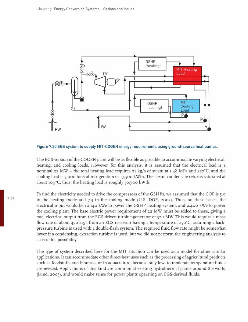
In the case of the MIT campus, the EGS system may be used in conjunction with ground­source heat pumps to provide all the heating and cooling needs (see Figure 7.20). The EGS system shown still allows for some direct heating using the back­pressure exhaust steam from the main turbine for those applications where steam is essential. In practice, these heating needs might be taken care of using steam bled from an appropriate stage of the turbine. Furthermore, because it is highly desirable to return the spent geofluid to the injection wells as cold as possible (to enhance the gravity­head flow effect), we still will use the liquid from the cyclone separator to meet some campus heating needs.

Chapter 7 Energy Conversion Systems – Options and Issues

PWIW

MIT Heating LoadT/G

GSHP(cooling)

GSHP(heating)

MITCoolingLoad

P

PP

Figure 7.20 EGS system to supply MIT­COGEN energy requirements using ground­source heat pumps. 

The EGS version of the COGEN plant will be as flexible as possible to accommodate varying electrical, heating,  and  cooling  loads.  However,  for  this  analysis,  it  is  assumed  that  the  electrical  load  is  a nominal 22 MW – the total heating load requires 21 kg/s of steam at 1.48 MPa and 227°C, and the cooling load is 5,000 tons of refrigeration or 17,500 kWth. The steam condensate returns saturated at about 109°C; thus, the heating load is roughly 50,700 kWth. 

To find the electricity needed to drive the compressors of the GSHPs, we assumed that the COP is 5.0 7­28 in  the  heating  mode  and  7.3  in  the  cooling  mode  (U.S.  DOE,  2005).  Thus,  on  these  bases,  the

electrical input would be 10,140 kWe to power the GSHP heating system, and 2,400 kWe to power the cooling plant. The base electric power requirement of 22 MW must be added to these, giving a total electrical output from the EGS­driven turbine­generator of 32.1 MW. This would require a mass flow rate of about 470 kg/s from an EGS reservoir having a temperature of 250°C, assuming a back­pressure turbine is used with a double­flash system. The required fluid flow rate might be somewhat lower if a condensing, extraction turbine is used, but we did not perform the engineering analysis to assess this possibility. 

The  type of  system described here  for  the MIT situation can be used as  a model  for other  similar applications. It can accommodate other direct­heat uses such as the processing of agricultural products such as foodstuffs and biomass, or in aquaculture, because only low­ to moderate­temperature fluids are needed. Applications of this kind are common at existing hydrothermal plants around the world (Lund, 2005), and would make sense for power plants operating on EGS­derived fluids.

Chapter 7 Energy Conversion Systems – Options and Issues

7.4 Plant Operational ParametersPower plants operating on EGS­derived geofluids will be subject to the same kind of operating and performance metrics  as  those at  conventional hydrothermal  resources. However, because  the EGS fluids are “pure” water to start with at the injection wells, and are recirculated after production, it is expected that they will be far less aggressive than typical hydrothermal fluids. This should minimize the problems often seen regarding chemical scaling, corrosion, and noncondensable gases found in some natural hydrothermal power plants where methods already exist  for  coping with all of  these potential problems. Nevertheless, the EGS fluids may have much higher pressures than those seen at hydrothermal  plants,  even  supercritical  pressures,  which  already  have  been  discussed.  These conditions, when combined with very high temperatures, will need to be accounted for in the field piping and plant design.

The  analysis  presented  here  presumes  that  the  properties  of  the  EGS  circulating  fluid  remain constant. Because this is unlikely to be true over the expected lifetime of a plant, it may be necessary to modify the plant components to maintain the power output, unless replacement wells are able to restore  the  initial  fluid  conditions.  This  problem  is  routinely  encountered  in  current  geothermal plants, both flash­steam and binary, and the methods used would apply to the EGS plants. 

The general finding is that no insurmountable difficulties are expected on the power­generation side of an EGS operation. 

7.5 Summary and ConclusionsIn this section, we have shown that:

• Energy conversion systems exist for use with fluids derived from EGS reservoirs.

• Conventional geothermal power plant techniques are available to cope with changing properties of the fluids derived from EGS reservoirs.

• It  is possible  to generate  roughly 6,000 MW of electricity  from fluids  that are currently being coproduced  from  oil  and  gas  operations  in  the  United  States  by  using  standard  binary­cycle technology.

• Power plant capital costs for coproduced fluids range from about $1,500­2,300/kW, depending on the temperature of the coproduced fluids.

• If a mass flow rate of 20 kg/s can be sustained from a 200°C EGS reservoir, approximately 1 MW of power can be produced; the same power can be achieved from a 250°C EGS reservoir, with only about 8.5 kg/s.

• Supercritical fluids from an EGS reservoir can be used in a triple­expansion power plant. About 15 kg/s will yield about 10 MW of power from fluids at 400°C and pressures in the range of 25­27 MPa; power plant thermal efficiencies will be about 31%.

• Supercritical fluids from an EGS reservoir at very high pressures up to 35 MPa and 400°C can be used in a single­expansion power plant to generate 10 MW of power from flow rates of 21­30 kg/s, depending on the fluid pressure.

7­29

Chapter 7 Energy Conversion Systems – Options and Issues

• Fluids derived from EGS reservoirs can be used  in  innovative cogeneration systems to provide electricity, heating, and cooling in conjunction with ground­source heat pumps. For example, the current MIT energy needs could be met with an EGS power plant with a 32 MW rating; this could be achieved with a flow rate of 1,760 kg/s from a 200°C EGS reservoir using a single­flash system – or a 470 kg/s flow rate from a 250°C EGS reservoir using a double­flash system – and back­pressure turbines.

• The  installed  specific  cost  ($/kW)  for  either  a  conventional  1­  or  2­flash  power  plant  at  EGS reservoirs  is  inversely dependent on  the  fluid  temperature and mass  flow rate. Over  the range from 150­340°C: For a mass flow rate of 100 kg/s, the specific cost varies from $1,894­1,773/kW (1­flash) and from $1,889­1,737/kW (2­flash); for a flow rate of 1,000 kg/s, the cost varies from $1,760­1,080/kW (1­flash) and from $1,718­981/kW (2­flash).

• The  total  plant  cost,  exclusive  of  wells,  for  a  2­flash  plant  receiving  1,000  kg/s  from  an  EGS reservoir would vary from $50 million to $260 million, with a fluid temperature ranging from 150­340°C; the corresponding power rating would vary from about 30­265 MW. If the reservoir were able to supply only 100 kg/s, the plant cost would vary from $5.6 million to $45.8 million over the same temperature range; the corresponding power rating would vary from 3­26.4 MW.

It should be noted that the possibility of using supercritical­pressure carbon dioxide as the circulating fluid  in  the  EGS  reservoir,  alluded  to  in  other  parts  of  this  report,  has  not  been  analyzed  in  this chapter.  The  use  of  CO2 as  the  heat­transfer  medium  raises  a  number  of  complex  questions,  the resolution of which lies beyond the scope of this report. The reader may consult Brown (2000) for an excellent discussion of this concept.

7­30

Chapter 7 Energy Conversion Systems – Options and Issues

ReferencesBrown, D.W. 2000. “A Hot Dry Rock Geothermal Energy Concept Utilizing Supercritical CO2 Instead of Water,” Proc. Twenty­Fifth Workshop on Geothermal Reservoir Engineering, Stanford University, Stanford, Calif., Jan. 24­26, 2000, SGP­TR­165.

Campbell, R.G. and M.M. Hatter. 1991. “Design and Operation of a Geopressured­Geothermal Hybrid Cycle Power Plant,” Final Report Vol. I, 180 pp. and Vol. II, 172 pp.; Eaton Operating Company Inc. and United States Department of Energy, The Ben Holt Co., DOE contract DE­ACO7­85ID12578.

Cooper, P. 2005. Peter Cooper, Manager of Sustainable Engineering/Utility Planning, MIT, personal communication, December 8.

Curtis, R., J. Lund, B. Sanner, L. Rybach, and G. Hellstrom. 2005. “Ground Source Heat Pumps – Geothermal  Energy  for  Anyone,  Anywhere:  Current  Worldwide  Activity,”  Proc.  World  Geothermal Congress, Antalya, Turkey, April 24­29.

DiPippo,  R.  2004.  “Second  Law  Assessment  of  Binary  Plants  for  Power  Generation  from  Low­Temperature Geothermal Fluids,” Geothermics, V. 33, pp. 565­586.

DiPippo, R. 2005. Geothermal Power Plants: Principles, Applications and Case Studies, Elsevier Advanced Technology, Oxford, England.

DOGGR.  2005.  2004  Annual  Report  of  the  State  Oil  &  Gas  Supervisor, California  Department  of Conservation, Div. of Oil, Gas, and Geothermal Resources, Sacramento, p. 197.

El Wakil, M.M. 1984. Powerplant Technology, McGraw­Hill, New York, pp. 71­72.

Griggs,  J.  2004.  “A Re­Evaluation  of  Geopressured­Geothermal  Aquifers  as  an  Energy  Resource,” Masters Thesis, Louisiana State University, The Craft and Hawkins Dept. of Petroleum Engineering, Baton Rouge, La., August 2004.

Lund, J.W. 2005. “Worldwide Utilization of Geothermal Energy – 2005,” GRC Transactions, V. 29, 7­31

pp. 831­836.

McKenna,  J.R.  and  D.D.  Blackwell.  2005.  “Geothermal  Electric  Power  From  Texas  Hydrocarbon Fields,” GRC BULLETIN, May/June, pp. 121­128.

McKenna, J.R., D.D. Blackwell, C. Moyes, and P.D. Patterson. 2005. “Geothermal Electric Power Supply Possible From Gulf Coast, Midcontinent Oil Field Waters,” Oil & Gas Journal, Sept. 5, pp. 34­40.

Moran,  M.J.  and  H.N.  Shapiro.  2004.  Fundamentals  of  Engineering  Thermodynamics,  5th  Ed., John Wiley & Sons, Hoboken, NJ.

Myers, J.E., L.M. Jackson, R.F. Bernier, and D.A. Miles. 2001. “An Evaluation of the Department of Energy  Naval  Petroleum  Reserve  No.  3  Produced  Water  Bio­Treatment  Facility,”  SPA/EPA/DOE Exploration and Production Environmental Conference, Paper No. SPE 66522, San Antonio, Texas, February 2001. 

Rybach, L. and H.L. Gorhan. 2005. “2005 Update for Switzerland,” Proc. World Geothermal Congress, Antalya, Turkey, April 24­29.

Chapter 7 Energy Conversion Systems – Options and Issues

Sanyal, S.K. 2005. “Levelized Cost of Geothermal Power – How Sensitive Is It?” GRC Transactions, V. 29, pp. 459­465.

Swanson, R.K. 1980. “Geopressured Energy Availability,” Final Report, EPRI AP­1457, Electric Power Research Institute, Palo Alto, Calif.

U.S.  DOE,  2005.  “How  to  Buy  an  Energy­Efficient  Ground  Source  Heat  Pump,” http://www.eere.energy.gov/femp/technologies/eep_groundsource_heatpumps.cfm.

Nomenclature (as used in figures) B Boiler BCV Ball check valve C Condenser; compressor (Fig. 7.18); Celsius (throughout) CC Combustion chamber CP Condensate pump CS  Cyclone separator CSV Control and stop valves CT Cooling tower CW  Cooling water CWP Cooling water pump E Evaporator EC Economizer F Flash vessel FF Final filter G Generator HPP High­pressure pump HPT High­pressure turbine HRSG Heat­recovery steam generator

7­32 IP IW LPP LPT M MR

Injection pump Injection well Low­pressure pump Low­pressure turbine Make­up water Moisture remover

P PH

Pump Preheater

PW Production well S Silencer SE/C SH SP SPT SR

Steam ejector/condenser Superheater Steam piping Super­pressure turbine Sand remover

T Turbine T/G TV

Turbine/generator Throttle valve

WP WV

Water piping Wellhead valve