
Overview of Next Gen Sequencing Data Analysis
73
January 7 th , 2015 Mariam Quiñones Computational Biology Specialist Bioinformatics and Computational Biosciences Branch Office of Cyber Infrastructure and Computational Biology
-
Upload
bcbbslides -
Category
Science
-
view
110 -
download
3
Transcript of Overview of Next Gen Sequencing Data Analysis
January 7th, 2015
Mariam Quiñones Computational Biology Specialist Bioinformatics and Computational Biosciences Branch Office of Cyber Infrastructure and Computational Biology
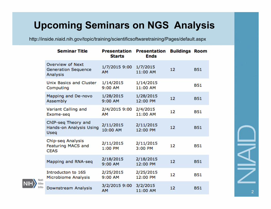
Upcoming Seminars on NGS Analysis
2
http://inside.niaid.nih.gov/topic/training/scientificsoftwaretraining/Pages/default.aspx
BCBB: A Branch Devoted to Bioinformatics and Computational Biosciences
Researchers’ time is increasingly important BCBB saves our collaborators time and effort Researchers speed projects to completion using
BCBB consultation and development services No need to hire extra post docs or use external
consultants or developers
3
BCBB Staff
4
Bioinformatics Software Developers Computational Biologists Project Managers and
Analysts
Contact BCBB…
“NIH Users: Access a menu of BCBB services on the NIAID Intranet: • http://bioinformatics.niaid.nih.gov/
Outside of NIH – • search “BCBB” on the NIAID Public Internet Page:
www.niaid.nih.gov – or – use this direct link
http://www.niaid.nih.gov/about/organization/odoffices/omo/ocicb/Pages/bcbb.aspx
Email us at: • [email protected]
5
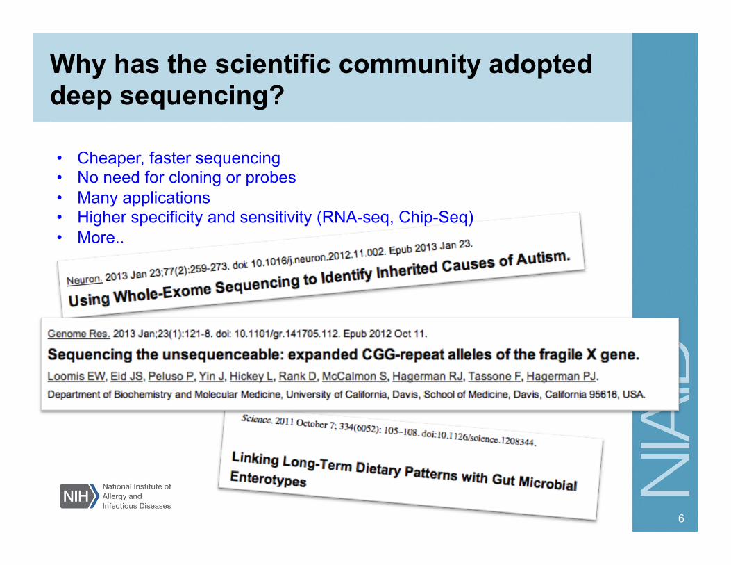
Why has the scientific community adopted deep sequencing?
6
• Cheaper, faster sequencing • No need for cloning or probes • Many applications • Higher specificity and sensitivity (RNA-seq, Chip-Seq) • More..

What is Next Generation Sequencing?
7
Image from: http://s.ngm.com/2009/06/tag-caves/img/01-rumbling-falls-615.jpg
It is sequencing produced by 2nd and 3rd generation instruments (e.g. Illumina, PacBio)”
• It is also known as High-Throughput Next Generation Sequencing (HT-NGS) or “Deep Sequencing”. Provides deeper coverage than the typical Sanger sequencing
Agenda for today
Overview of Next Generation Sequencing NGS sequencing platforms NGS Analysis Basics
• File formats • Quality Control • Viewing alignment files
Common applications of NGS
8
Remember Sanger?
9
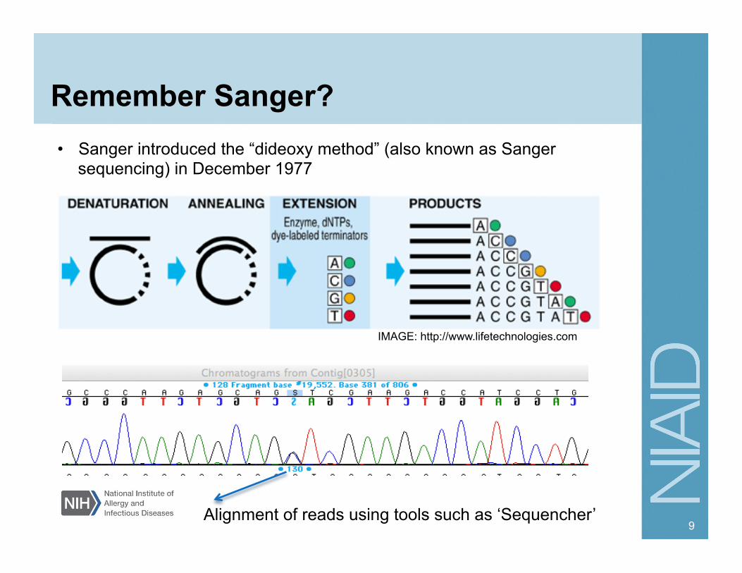
• Sanger introduced the “dideoxy method” (also known as Sanger sequencing) in December 1977
Alignment of reads using tools such as ‘Sequencher’
IMAGE: http://www.lifetechnologies.com

Sanger Next Generation Sequencing
10
• Sanger: Dideoxy Chain Termination 1977
• Hood et al., Fluorescently labeled ddNTPs, Partial Automation 1986
• NIH begins Human Genome Project, 1990
• HGP/Celera draft assembly published Nature / Science 2001
• Next-Gen Sequencing (454 Roche) 2004
• First Solexa Sequencer, Genome Analyzer 1G/Run 2006
• 1990 – 2003 • “shotgun”
2007 J.Craig Venter James Watson
Greater vision: Genomics to Bedside
“ Only a population perspective can fulfill the promise of genomic medicine. The scientific landscape for genomics is exciting, and the promise for improving health is great. Applying genomic tools in clinical and public health practice will require a multidisciplinary research collaboration of basic sciences with clinical and population sciences (e.g., epidemiologists; behavioral, social, and communication scientists; health services researchers; and public health practitioners)”
Am J Public Health. 2012 January; 102(1): 34–37
11
Popular Sequencing Platforms (non-Illumina)
12
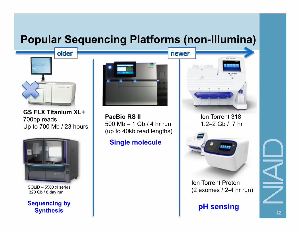
SOLiD – 5500 xl series 320 Gb / 8 day run
GS FLX Titanium XL+ 700bp reads Up to 700 Mb / 23 hours
PacBio RS II 500 Mb – 1 Gb / 4 hr run (up to 40kb read lengths)
Ion Torrent 318 1.2–2 Gb / 7 hr
pH sensing Sequencing by Synthesis
Single molecule
Ion Torrent Proton (2 exomes / 2-4 hr run)
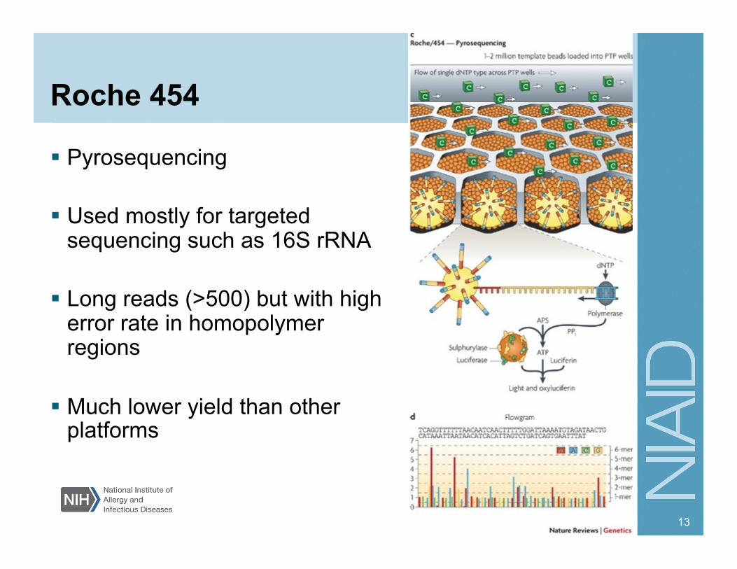
Roche 454
Pyrosequencing Used mostly for targeted
sequencing such as 16S rRNA Long reads (>500) but with high
error rate in homopolymer regions
Much lower yield than other platforms
13
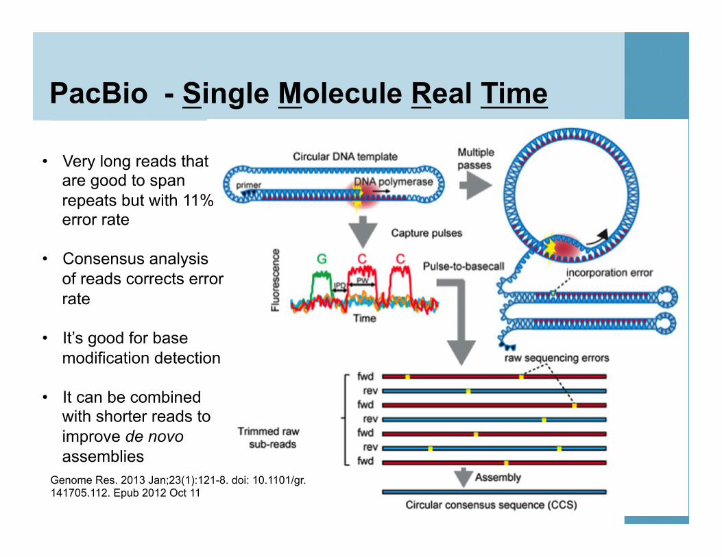
PacBio - Single Molecule Real Time
14
• Very long reads that are good to span repeats but with 11% error rate
• Consensus analysis of reads corrects error rate
• It’s good for base
modification detection
• It can be combined with shorter reads to improve de novo assemblies
Genome Res. 2013 Jan;23(1):121-8. doi: 10.1101/gr.141705.112. Epub 2012 Oct 11

Ion Torrent sequence detection
15
http://en.wikipedia.org/wiki/Ion_semiconductor_sequencing
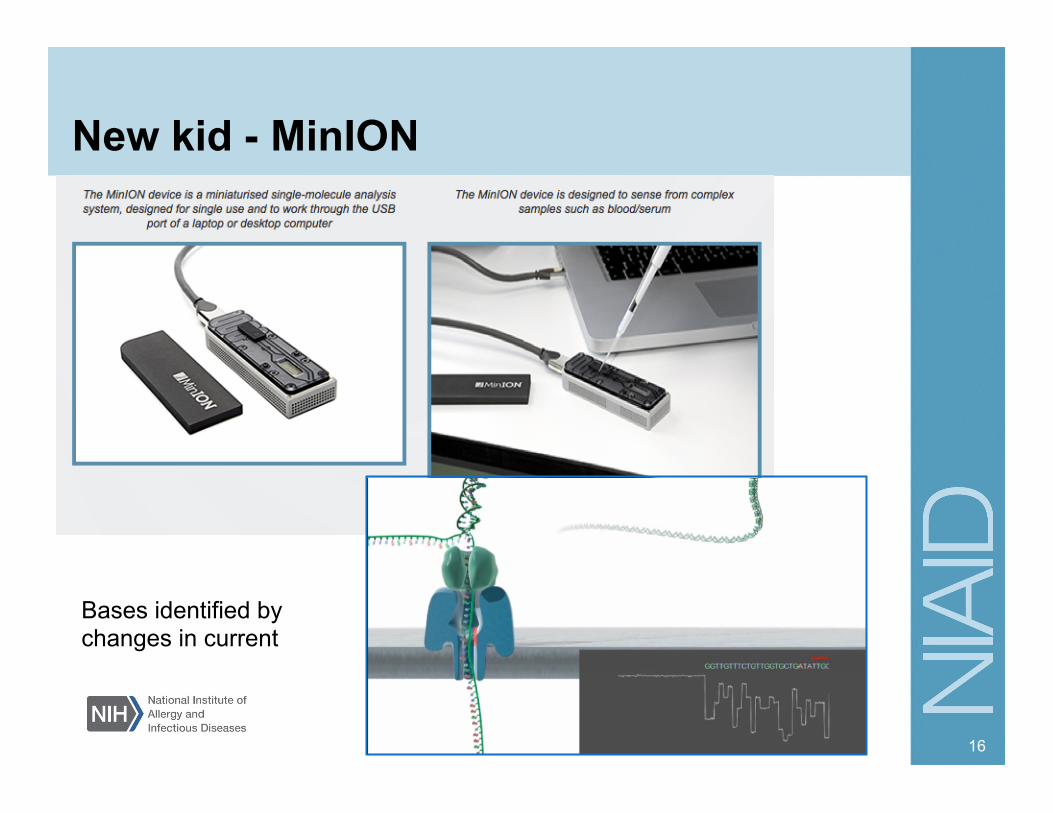
New kid - MinION
16
Bases identified by changes in current

Illumina platforms
17
ILLUMINA
18
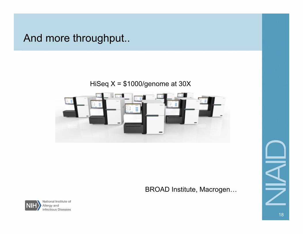
HiSeq X = $1000/genome at 30X
And more throughput..
BROAD Institute, Macrogen…
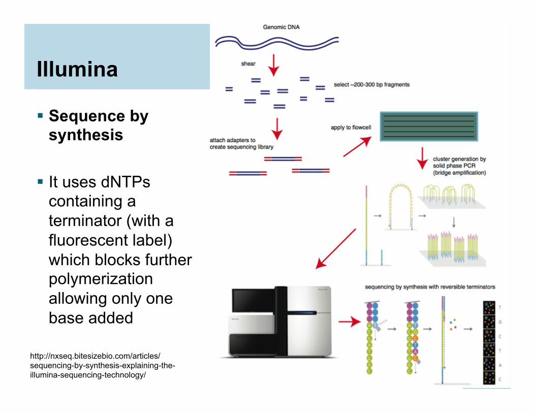
Illumina
Sequence by synthesis
It uses dNTPs
containing a terminator (with a fluorescent label) which blocks further polymerization allowing only one base added
19
http://nxseq.bitesizebio.com/articles/sequencing-by-synthesis-explaining-the-illumina-sequencing-technology/
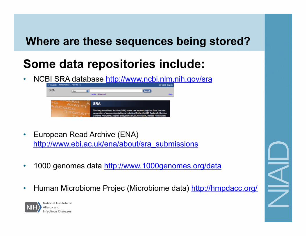
Where are these sequences being stored?
• NCBI SRA database http://www.ncbi.nlm.nih.gov/sra
• European Read Archive (ENA)
http://www.ebi.ac.uk/ena/about/sra_submissions
• 1000 genomes data http://www.1000genomes.org/data • Human Microbiome Projec (Microbiome data) http://hmpdacc.org/
Some data repositories include:
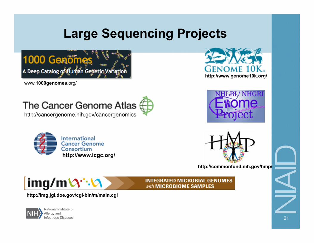
Large Sequencing Projects
21
http://cancergenome.nih.gov/cancergenomics
www.1000genomes.org/
http://commonfund.nih.gov/hmp/
http://www.icgc.org/
http://img.jgi.doe.gov/cgi-bin/m/main.cgi
http://www.genome10k.org/
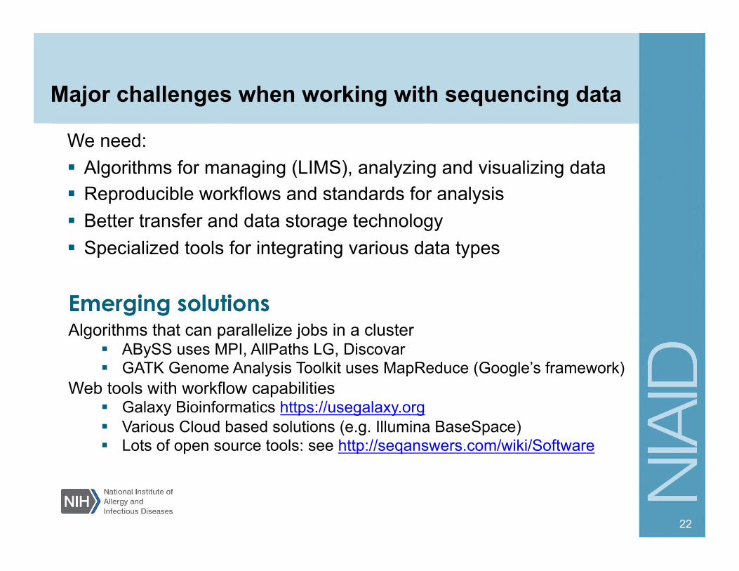
Major challenges when working with sequencing data
We need: Algorithms for managing (LIMS), analyzing and visualizing data Reproducible workflows and standards for analysis Better transfer and data storage technology Specialized tools for integrating various data types
22
Emerging solutions Algorithms that can parallelize jobs in a cluster
ABySS uses MPI, AllPaths LG, Discovar GATK Genome Analysis Toolkit uses MapReduce (Google’s framework)
Web tools with workflow capabilities Galaxy Bioinformatics https://usegalaxy.org Various Cloud based solutions (e.g. Illumina BaseSpace) Lots of open source tools: see http://seqanswers.com/wiki/Software

Galaxy https://usegalaxy.org
Makes analysis methods available to the community and facilitates reproducibility via creation of reusable workflows (read Galaxy slides)
Free web service, also compatible with Cloud http://usegalaxy.org/cloud
Open source
Provides a Genome Track Browser to visualize custom data.
23
Cartoons from: fixingpcerrors.com and squido.com
I have data, where do I start?
First the basics – NGS 101
Sequence data • What does a short read looks like? • How to know if sequencer facility has
provided good quality reads? • What to expect if sequencer facility has
mapped the reads to my genome of interest?
25
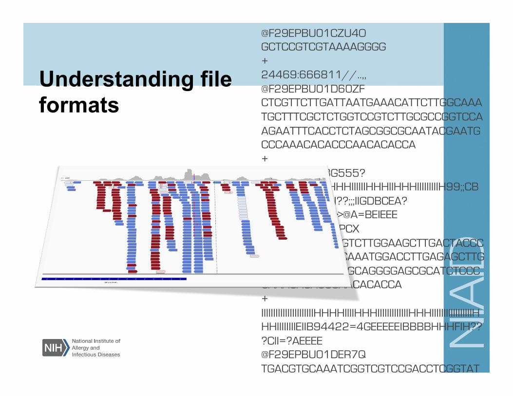
Understanding file formats
@F29EPBU01CZU4O GCTCCGTCGTAAAAGGGG + 24469:666811//..,, @F29EPBU01D60ZF CTCGTTCTTGATTAATGAAACATTCTTGGCAAATGCTTTCGCTCTGGTCCGTCTTGCGCCGGTCCAAGAATTTCACCTCTAGCGGCGCAATACGAATGCCCAAACACACCCAACACACCA + G???HHIIIIIIIIIBG555?=IIIIIIIIHHGHHIHHHIIIIIIHHHIIHHHIIIIIIIIIH99;;CBBCCEI???DEIIIIII??;;;IIGDBCEA?9944215BB@>>@A=BEIEEE @F29EPBU01EIPCX TTAATGATTGGAGTCTTGGAAGCTTGACTACCCTACGTTCTCCTACAAATGGACCTTGAGAGCTTGTTTGGAGGTTCTAGCAGGGGAGCGCATCTCCCCAAACACACCCAACACACCA + IIIIIIIIIIIIIIIIIIIIIIHHHHIIIIHHHIIIIIIIIIIIIIHHHIIIIIIIIIIIIIIIIIHHHIIIIIIIIEIIB94422=4GEEEEEIBBBBHHHFIH???CII=?AEEEE @F29EPBU01DER7Q TGACGTGCAAATCGGTCGTCCGACCTCGGTATAGGGGCGAAGACTAATCGAACCATCTAGTAGCTGGTT + IIIIIIIG666GIIIIIIIIIIIIIIIIIIIII====:2:::<EEIIIIIIIIIIIIIIIIIGGGIIII @F29EPBU01B2FE3 TCAACGATTAAAGTCCTACGTGATCTGAGTTCAGACCGGAGCAATCCAGGTCGGTTTCTATCTATTCAACATTTCTCCCTGTACGAAAGGACAAGAGAAATAGGGCCCACTTCACAATAGCGCCCNCCNCCNCCACACACACACACAC + ADBBBBD?B666FFFFHHHIFFFFFFFFFFFFFC86666DDDDDBBDFFFFFFF???FFFFCAA>ABBBB=336:<F??DDDDFFFFFDD?A===BA111?688;;;;?<:::<?>>?>?980..!//!86!669888??=<999822 @F29EPBU01BD6BJ GTTGTAGGTCGGTAGTGTCGTCGGTAC + 80006:;<4/..9:233342225984/ @F29EPBU01DDR5H TGTGATGTGTCTTTATAGTAGCATGATTTATAATCCTTTGGGTATATACTCAATAATGGGATCACTGGGTCAAATGGA + ADDBBBDHHHF:::FFGGDDDDDDBB;44498411144;555ABDFFFFFFFFFFFFFFFF???A?=:88>8889889 @F29EPBU01BXIBN GTGGAGGTCCGTAGCGGTCTTGACGTGCAAATCGGTCGTCCGACCTGGGTATAGGGGCGG + HIIIIIIIIIIIIIIIIIIIIIIIIIIIHHHIIIIIIIIIIIIBBCDEBEE;8/---0,, @F29EPBU01EMLVL TACCTCGCTGACTGACTGACTGACTGACTGACTGACTGACTGACTGACTGACTGACTCGCCAAACACACCC + IIIIIIIIIIIIIIIIIIIIIIIIIIIIIIIIIIIIIIIIIIIIIIIIIIIIIIIIIIGFDB@@E?E<333 @F29EPBU01DHVGX TGGTGGCGTACT + :662114,//// @F29EPBU01DSSQC CGATCTGATAAATGCACGCATCCCNCC + BAAAAAB@6666?ABA??===862!,, @F29EPBU01A3JW3 GGGAGTCGGGGAGTTGCAATTAATTTCCCCACCT + 44271::....71;9676;688886622227/// @F29EPBU01CTSZ0 CGTGGGTGCGC + 43422230422 @F29EPBU01EIWX8 TGGGGCTGGAATTACCGCGGCTGCTGGCACCAGACTTGCCCTCCAATGGATCCTCGTTAAAGGATTTAAAGTGGACTCATTCCAATTACAGGGCCTCGA + A1111@@EEEEGEEHHIIIIIIIIIIIIIIIIIIIIIIHHHIGGHHIHHHIIIIIIIIHHHIIIHHHHHHIIIIIIIIIIIIIIIIIIII???HHIIII @F29EPBU01DP0LM TGCGTGGGCGATTGTCTGGTTAATTCCGATAACGAACGAGACTCTCCCA + >@>=>444<042276=<222244===89998AABBBDBBAA?A?@;84/ @F29EPBU01DSYYK GTGTAGTGATATCG + :::89863445244 @F29EPBU01CLHKI GTCTCGTTCGTTATCGGAATTAACCAGACAAATCGCTCCACCAAATAAGAACGCCAAACACACCCAACC + IIIIIIHHIIIIIII====>>IIIIIIIIEBBGGGFG;7542??@E???::<@FF765A=AA===1/., @F29EPBU01AYJ2F TCTCTTAGTCATAGTGA + FFFHGIIIIIIIIIIII @F29EPBU01DVTHA TGCGTCGTGGTTAGAATTCCTATAGGTAATACG + 100//6<=112242<<<<992448?<<2232:7 @F29EPBU01A4RY6 TGTAGGTAGGGACAGTGGGAATCTCGTTCATCCATTCATGCGCGTCACTAATTAGATGACGAGGCATTTTGGCTACCTTAAGAGAGTCATAGTTACT + 145IHHII<<>GIIIIHHHIIIIIIIIIIIIIIIGGGIIIIIIIIIIIIIIIIIIIIIIIHGEED>111///=A=4445@AIIIIIIIIIHIHEGA9 @F29EPBU01D9UUA GACAGCTCTTTAGACACTAGGAAAACCTTATATAGAGNGTAAAAGCATAACCACCATAGTTAGCCCAAAAGCAGCCATC + HIIIIIIHHEEIIIII==99:BBBBIIIIFIIIIIBB!@@====B?<<;@@@DDEEEGG@@@F>>>AABBIIIIIIIB@ @F29EPBU01C0T3C GGTATAGT
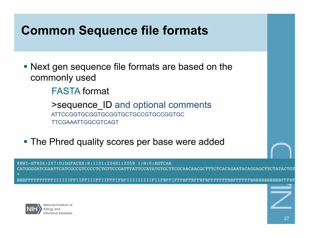
Common Sequence file formats
Next gen sequence file formats are based on the commonly used
FASTA format >sequence_ID and optional comments ATTCCGGTGCGGTGCGGTGCTGCCGTGCCGGTGC TTCGAAATTGGCGTCAGT
The Phred quality scores per base were added
27
@HWI-ST406:207:D1DGFACXX:8:1101:20481:2058 1:N:0:AGTCAA!CATGGGGATCGAATTCATCGCCGTCCCCTCTGTTCCGATTTATTCCATATGTGCTTCGCAACAACGCTTTCTCACAGAATACAGGAGCTTCTATACTGTA!+!BBBFFFFFFFFFFIIIIIIFFIIFFIIIFFIIFFFIFBFIIIIIIIIIFIIFBFFIFFFBFFBFFBFBFFFFFFFBBFFFFFFBBBBBBBBBBBFFFBFB!
Raw sequence file formats
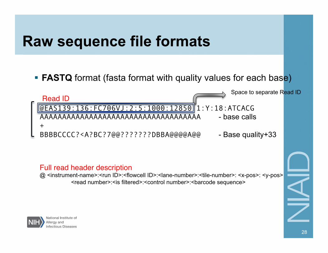
FASTQ format (fasta format with quality values for each base)
28
@EAS139:136:FC706VJ:2:5:1000:12850 1:Y:18:ATCACG AAAAAAAAAAAAAAAAAAAAAAAAAAAAAAAAAAAA - base calls + BBBBCCCC?<A?BC?7@@???????DBBA@@@@A@@ - Base quality+33
Full read header description"@ <instrument-name>:<run ID>:<flowcell ID>:<lane-number>:<tile-number>: <x-pos>: <y-pos>
<read number>:<is filtered>:<control number>:<barcode sequence>
Space to separate Read ID Read ID "
Quality values
29
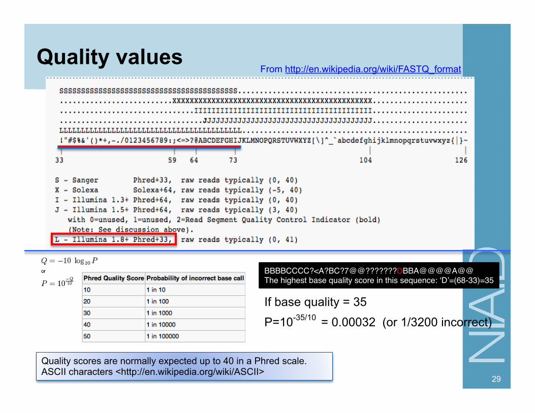
Quality scores are normally expected up to 40 in a Phred scale. ASCII characters <http://en.wikipedia.org/wiki/ASCII>
BBBBCCCC?<A?BC?7@@???????DBBA@@@@A@@ "The highest base quality score in this sequence: ‘D’=(68-33)=35
From http://en.wikipedia.org/wiki/FASTQ_format
= 0.00032 (or 1/3200 incorrect) P=10-35/10
If base quality = 35
Other read formats
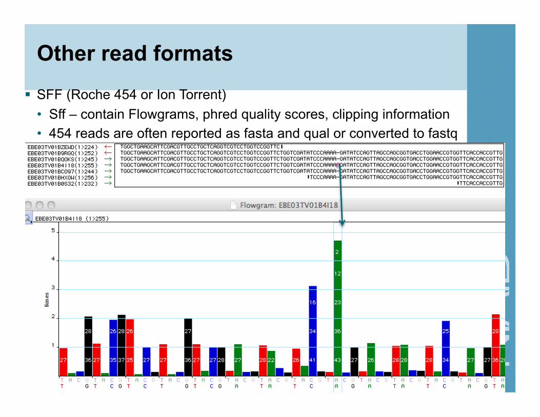
SFF (Roche 454 or Ion Torrent) • Sff – contain Flowgrams, phred quality scores, clipping information • 454 reads are often reported as fasta and qual or converted to fastq
30
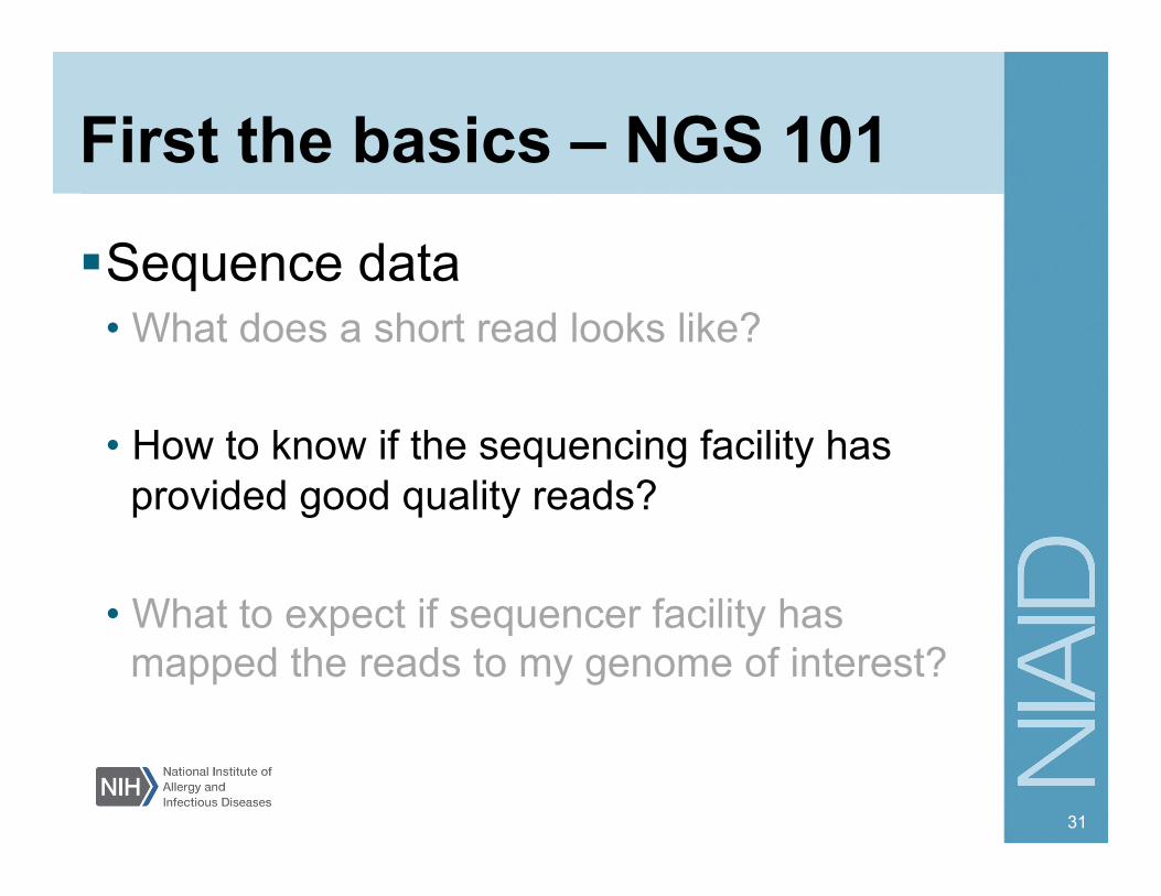
First the basics – NGS 101
Sequence data • What does a short read looks like? • How to know if the sequencing facility has
provided good quality reads? • What to expect if sequencer facility has
mapped the reads to my genome of interest?
31

Basic Concepts in Quality Control of sequence data
The sequencing facility runs quality control tests to ensure that the actual run was successful and/or to determine if a new library is good for sequencing more of it.
The user should run quality control tests prior to full bioinformatics
analyses • This will avoid misinterpretation of the data due to unexpected bias • QC measurements can report the following:
– Percent GC in sample reads – Presence of overrepresented kmers and sequences such as adapters – Per base quality score – Distribution of nucleotide bases
After mapping reads to a genome, additional test could be run to
determine: – Mapping error rate – Percent of possible PCR duplicates (reads with same start and end position in
reference genome) – Distribution of insert size (pair ends)
32
Demo – Fastq Quality
33
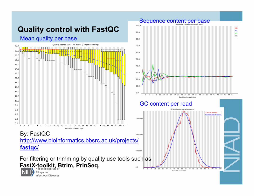
Quality control with FastQC
By: FastQC http://www.bioinformatics.bbsrc.ac.uk/projects/fastqc/
Mean quality per base
Sequence content per base
GC content per read
For filtering or trimming by quality use tools such as FastX-toolkit, Btrim, PrinSeq.
First the basics – NGS 101
Sequence data • What does a short read looks like? • How to know if the sequencing facility has
provided good quality reads? • What to expect if sequencing facility has
mapped (aligned) the reads to my genome of interest?
35
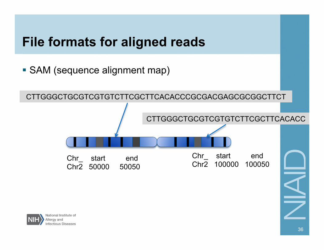
File formats for aligned reads
SAM (sequence alignment map)
36
CTTGGGCTGCGTCGTGTCTTCGCTTCACACCCGCGACGAGCGCGGCTTCT
CTTGGGCTGCGTCGTGTCTTCGCTTCACACC
Chr_ start end Chr2 100000 100050
Chr_ start end Chr2 50000 50050

Most commonly used alignment file formats SAM (sequence alignment map) Unified format for storing alignments to a reference genome BAM (binary version of SAM) – used commonly to deliver data
Compressed SAM file, is normally indexed BED Commonly used to report features described by chrom, start, end, name, score, and strand.
For example: chr1 11873 14409 uc001aaa.3 0 +
37
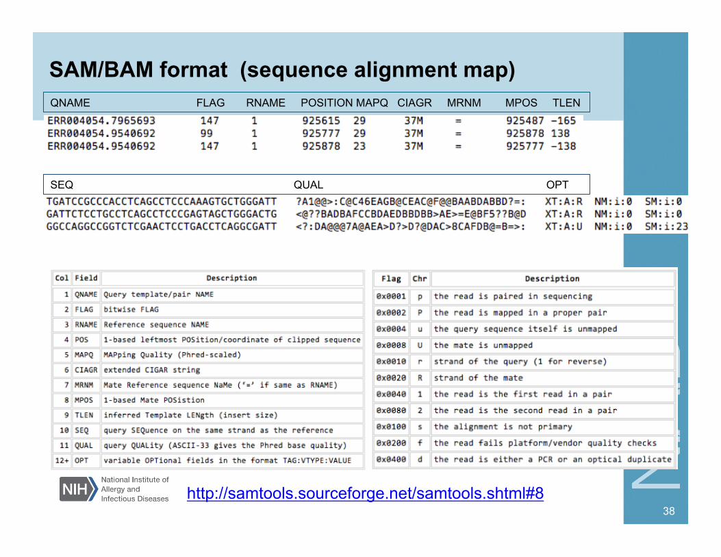
SAM/BAM format (sequence alignment map)
38
QNAME FLAG RNAME POSITION MAPQ CIAGR MRNM MPOS TLEN
SEQ QUAL OPT
http://samtools.sourceforge.net/samtools.shtml#8
First the basics – NGS 101
How to visualize an alignment? • Use a genome browser
39
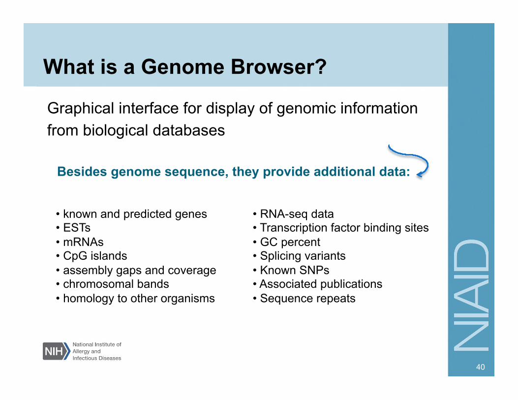
What is a Genome Browser?
Graphical interface for display of genomic information from biological databases
• known and predicted genes • ESTs • mRNAs • CpG islands • assembly gaps and coverage • chromosomal bands • homology to other organisms
• RNA-seq data • Transcription factor binding sites • GC percent • Splicing variants • Known SNPs • Associated publications • Sequence repeats
Besides genome sequence, they provide additional data:
40
Viewing reads in browser If your genome is available via the UCSC genome
browser http://genome.ucsc.edu/, import bam format file to the UCSC genome browser by hosting the file on a server and providing the link.
If your genome is not in UCSC, use another browser
such as IGV http://www.broadinstitute.org/igv/ , or IGB http://bioviz.org/igb/ • Import genome (fasta) • Import annotations (gff3 or bed format) • Import data (bam)

Data from ENCODE, Expression (RNA-Seq), Methylation and Transcription Factor binding (Chip-Seq) and more.
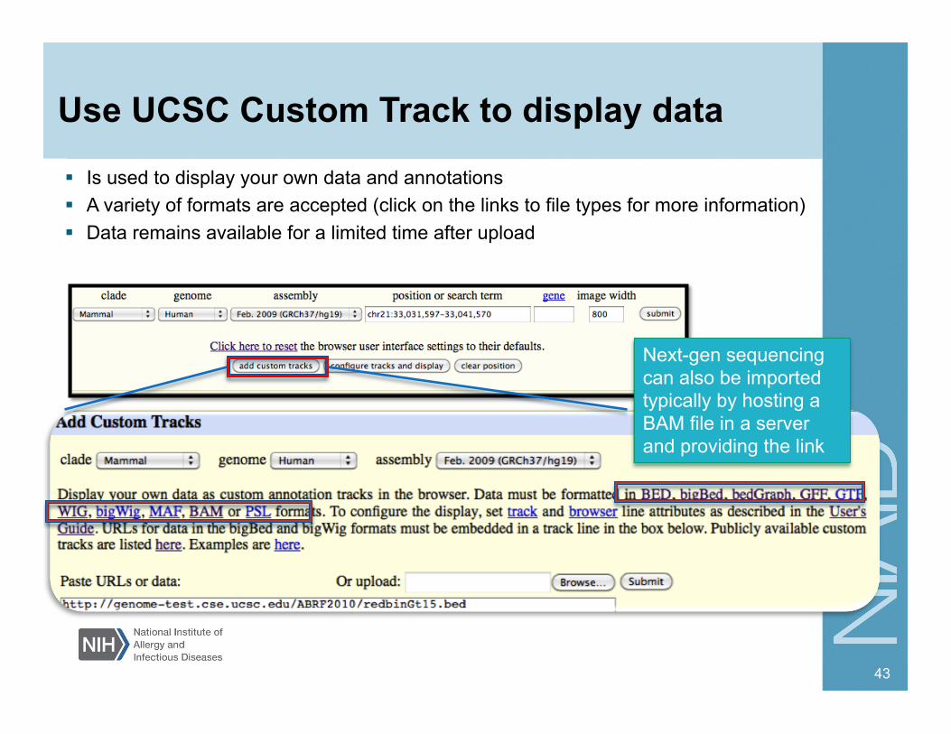
Use UCSC Custom Track to display data
Next-gen sequencing can also be imported typically by hosting a BAM file in a server and providing the link
Is used to display your own data and annotations A variety of formats are accepted (click on the links to file types for more information) Data remains available for a limited time after upload
43
Java tool that runs in user’s computer Allows for upload of custom annotations in many
formats • Add your genome (for example P. falciparum latest
version) in fasta format. • Add gene expression (gct format) or sequence
alignments (bam format). • Add custom annotations (bed, wig format, gff3).
Integrative Genomics Viewer (IGV) http://www.broadinstitute.org/igv/
44
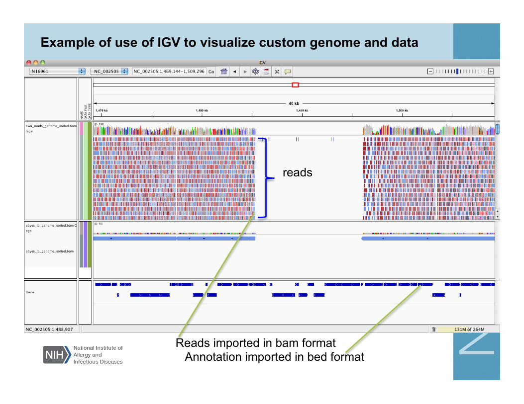
Example of use of IGV to visualize custom genome and data
Reads imported in bam format Annotation imported in bed format
reads
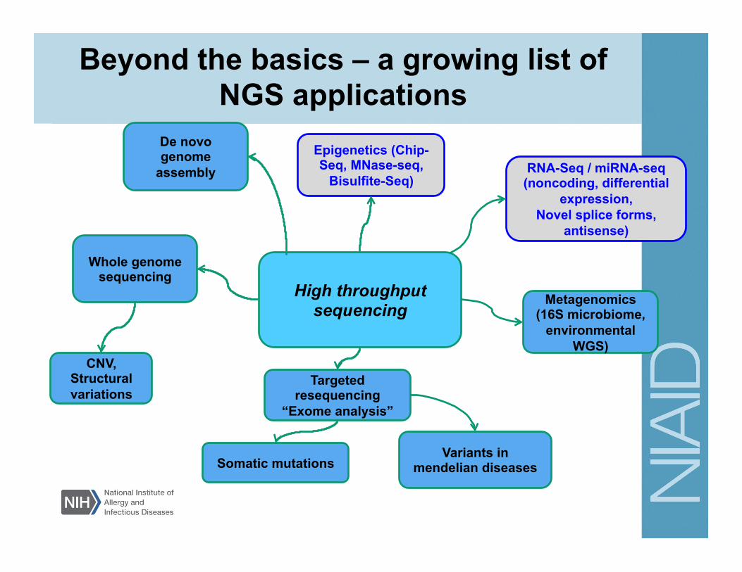
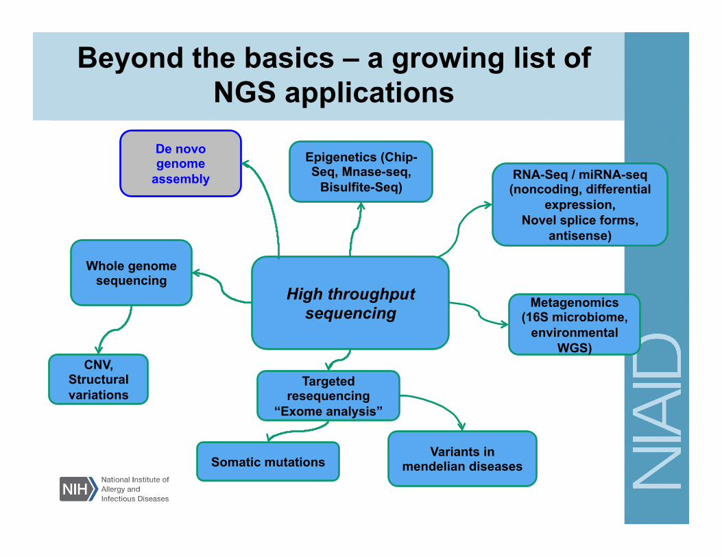
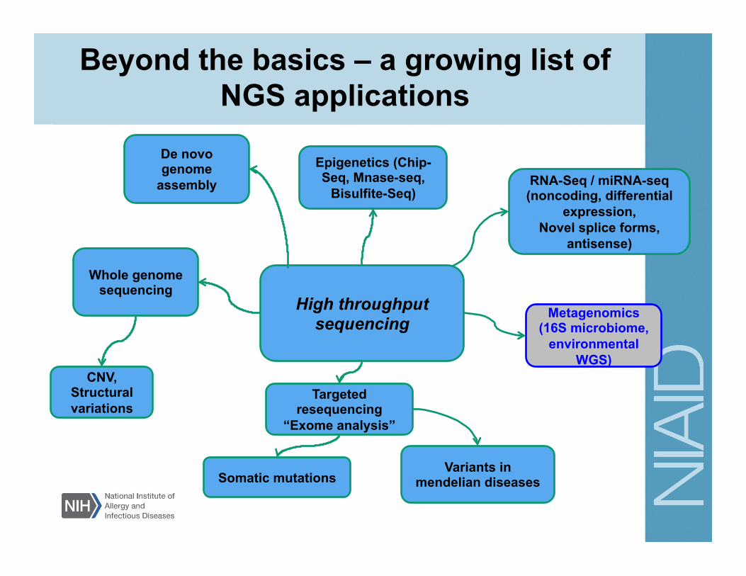
RNA-Seq / miRNA-seq (noncoding, differential
expression, Novel splice forms,
antisense)
Epigenetics (Chip-Seq, MNase-seq,
Bisulfite-Seq)
CNV, Structural variations
Targeted resequencing
“Exome analysis”
Whole genome sequencing
Metagenomics (16S microbiome,
environmental WGS)
Somatic mutations Variants in
mendelian diseases
High throughput sequencing
De novo genome
assembly
Beyond the basics – a growing list of NGS applications
47
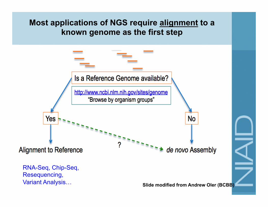
RNA-Seq, Chip-Seq, Resequencing, Variant Analysis…
Most applications of NGS require alignment to a known genome as the first step
Slide modified from Andrew Oler (BCBB)

How to align reads to a genome?
Step 1: Choose an appropriate alignment software http://seqanswers.com/wiki/Software
• Common tools: – Bowtie: FAST, Accurate (e.g. for Chip-Seq) – BWA: FAST, Accurate, gapped alignment (variant analysis) – TopHat: Uses Bowtie for initial mapping and then maps
junctions (good for RNA-seq mapping) – GSMapper, MIRA: developed for 454 Roche data – QIIME, mothur: Suite for processing and alignment of 16S
rRNA amplicon data for microbiome
48
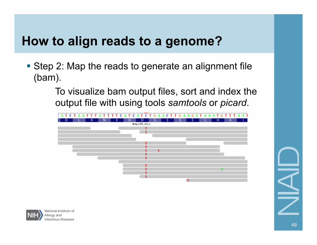
How to align reads to a genome?
Step 2: Map the reads to generate an alignment file (bam).
To visualize bam output files, sort and index the output file with using tools samtools or picard.
49
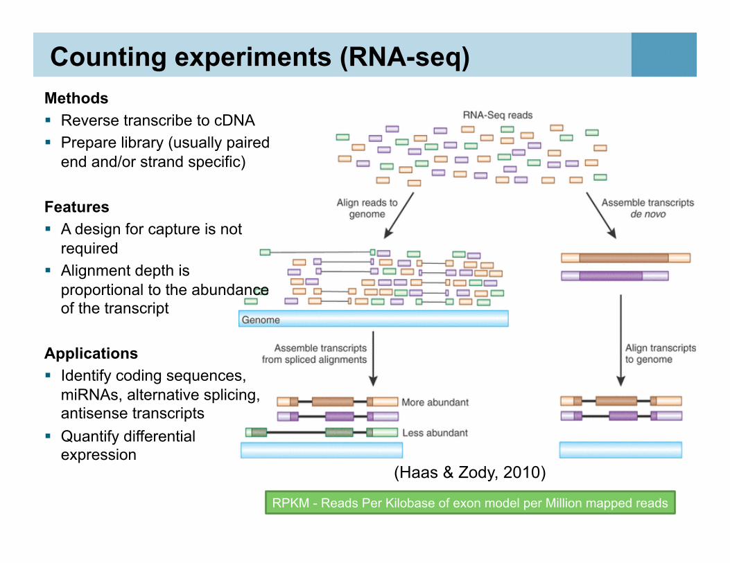
Counting experiments (RNA-seq) Methods Reverse transcribe to cDNA Prepare library (usually paired
end and/or strand specific)
Features A design for capture is not
required Alignment depth is
proportional to the abundance of the transcript
Applications Identify coding sequences,
miRNAs, alternative splicing, antisense transcripts
Quantify differential expression
50 RPKM - Reads Per Kilobase of exon model per Million mapped reads
(Haas & Zody, 2010)
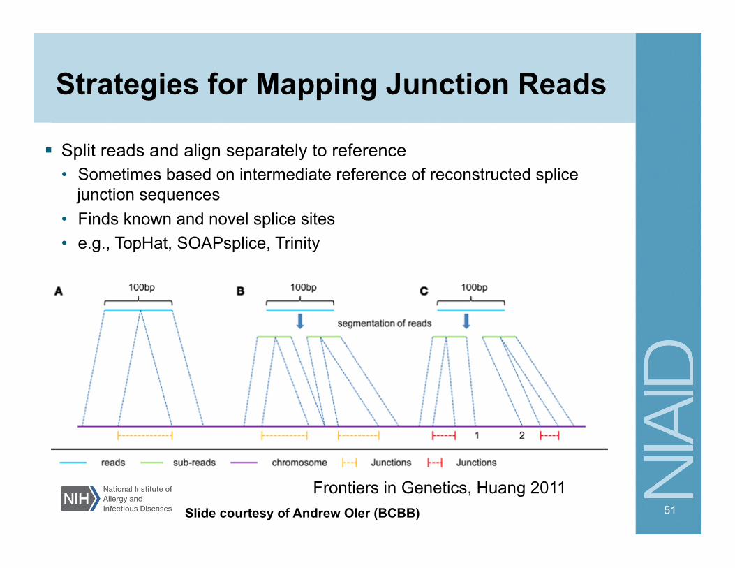
Strategies for Mapping Junction Reads
Split reads and align separately to reference • Sometimes based on intermediate reference of reconstructed splice
junction sequences • Finds known and novel splice sites • e.g., TopHat, SOAPsplice, Trinity
51
Frontiers in Genetics, Huang 2011 Slide courtesy of Andrew Oler (BCBB)
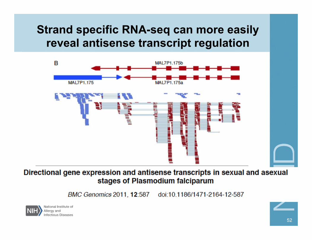
Strand specific RNA-seq can more easily reveal antisense transcript regulation
52
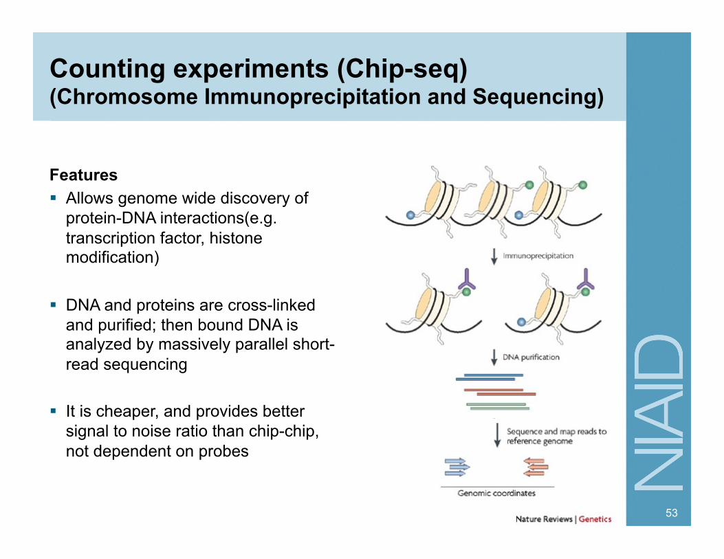
Counting experiments (Chip-seq) (Chromosome Immunoprecipitation and Sequencing)
Features Allows genome wide discovery of
protein-DNA interactions(e.g. transcription factor, histone modification)
DNA and proteins are cross-linked and purified; then bound DNA is analyzed by massively parallel short-read sequencing
It is cheaper, and provides better signal to noise ratio than chip-chip, not dependent on probes
53
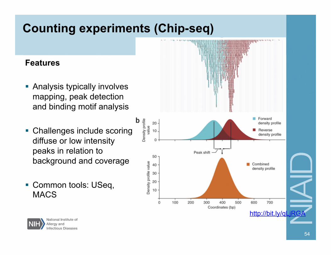
Counting experiments (Chip-seq)
Features Analysis typically involves
mapping, peak detection and binding motif analysis
Challenges include scoring diffuse or low intensity peaks in relation to background and coverage
Common tools: USeq, MACS
54
http://bit.ly/qLjRGA
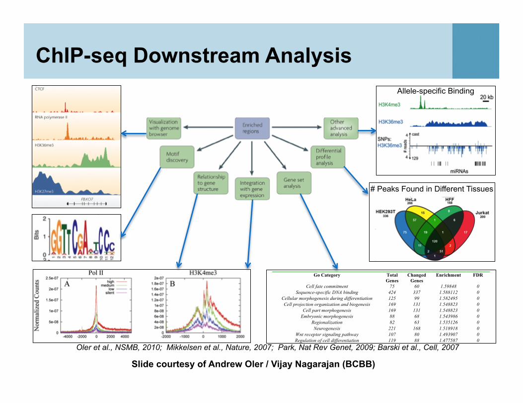
ChIP-seq Downstream Analysis
55
Supplemental Table 2: D1 Histone-enriched loci (Illumina GAII FDR< 0.0001)
Go Category Total
Genes
Changed
Genes
Enrichment FDR
Cell fate commitment 75 60 1.59848 0
Sequence-specific DNA binding 424 337 1.588112 0
Cellular morphogenesis during differentiation 125 99 1.582495 0
Cell projection organization and biogenesis 169 131 1.548823 0
Cell part morphogenesis 169 131 1.548823 0
Embryonic morphogenesis 88 68 1.543986 0
Regionalization 82 63 1.535126 0
Neurogenesis 221 168 1.518918 0
Wnt receptor signaling pathway 107 80 1.493907 0
Regulation of cell differentiation 119 88 1.477587 0
Regulation of transcription from RNA polymerase II
promoter
99 72 1.453164 0
Organ morphogenesis 304 221 1.452566 0
Embryonic development 226 164 1.449949 0
Regulation of developmental process 191 138 1.443653 0
Voltage-gated ion channel activity 171 123 1.43723 0
Nervous system development 604 433 1.432413 0
Cation channel activity 228 162 1.419703 0
Transcription factor activity 791 552 1.394376 0
Muscle development 136 94 1.38104 0
Central nervous system development 190 129 1.356605 0
Skeletal development 193 130 1.34587 0
Anatomical structure morphogenesis 855 575 1.343751 0
System development 1396 934 1.336838 0
Multicellular organismal development 1868 1248 1.334919 0
Channel or pore class transporter activity 363 242 1.332067 0
Enzyme linked receptor protein signaling pathway 228 152 1.332067 0
Positive regulation of transcription DNA-dependent 180 120 1.332067 0
Cell morphogenesis 374 249 1.330286 0
Cell Differentiation 1437 874 1.330286 0
Positive regulation of transcription 227 151 1.329133 0
Anatomical structure development 1679 1107 1.317389 0
Positive regulation of cell proliferation 192 126 1.311253 0
Organ development 996 650 1.303981 0
Cell fate commitment 75 60 1.59848 0
Sequence-specific DNA binding 424 337 1.588112 0
Cellular morphogenesis during differentiation 125 99 1.582495 0
Positive regulation of biological process 850 513 1.548823 0
51674 localization of cell 324 203 1.251896 0
32502 developmental process 2619 1639 1.250434 0
06812 cation transport 432 270 1.248812 0
15075 ion transporter activity 622 387 1.243191 0
42127 regulation of cell proliferation 383 238 1.241639 0
65009 regulation of a molecular function 400 246 1.228831 0
06366 transcription from RNA polymerase II
promoter
532 326 1.2244 0
50790 regulation of catalytic activity 381 233 1.221935 0
05576 extracellular region 1056 596 1.127716 0
06351 transcription DNA-dependent 1866 1050 1.124333 0
www.nature.com / nature 2
# Peaks Found in Different Tissues
Allele-specific Binding
Oler et al., NSMB, 2010; Mikkelsen et al., Nature, 2007; Park, Nat Rev Genet, 2009; Barski et al., Cell, 2007
Slide courtesy of Andrew Oler / Vijay Nagarajan (BCBB)
Are you still awake?
56
RNA-Seq / miRNA-seq (noncoding, differential
expression, Novel splice forms,
antisense)
Epigenetics (Chip-Seq, Mnase-seq,
Bisulfite-Seq)
CNV, Structural variations
Targeted resequencing
“Exome analysis”
Whole genome sequencing
Metagenomics (16S microbiome,
environmental WGS)
Somatic mutations Variants in
mendelian diseases
High throughput sequencing
De novo genome
assembly
Beyond the basics – a growing list of NGS applications
De novo genome assembly
58
AllPATHS-LG http://www.broadinstitute.org/news/2787
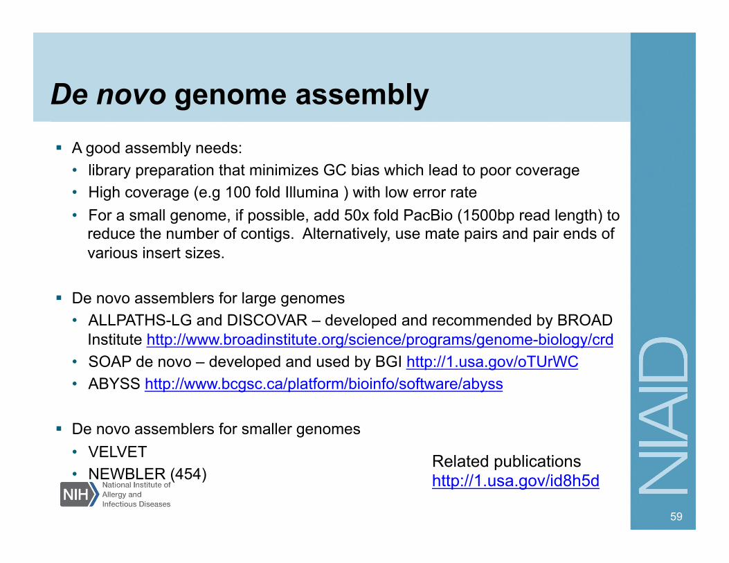
De novo genome assembly A good assembly needs:
• library preparation that minimizes GC bias which lead to poor coverage • High coverage (e.g 100 fold Illumina ) with low error rate • For a small genome, if possible, add 50x fold PacBio (1500bp read length) to
reduce the number of contigs. Alternatively, use mate pairs and pair ends of various insert sizes.
De novo assemblers for large genomes • ALLPATHS-LG and DISCOVAR – developed and recommended by BROAD
Institute http://www.broadinstitute.org/science/programs/genome-biology/crd • SOAP de novo – developed and used by BGI http://1.usa.gov/oTUrWC • ABYSS http://www.bcgsc.ca/platform/bioinfo/software/abyss
De novo assemblers for smaller genomes
• VELVET • NEWBLER (454)
59
Related publications http://1.usa.gov/id8h5d
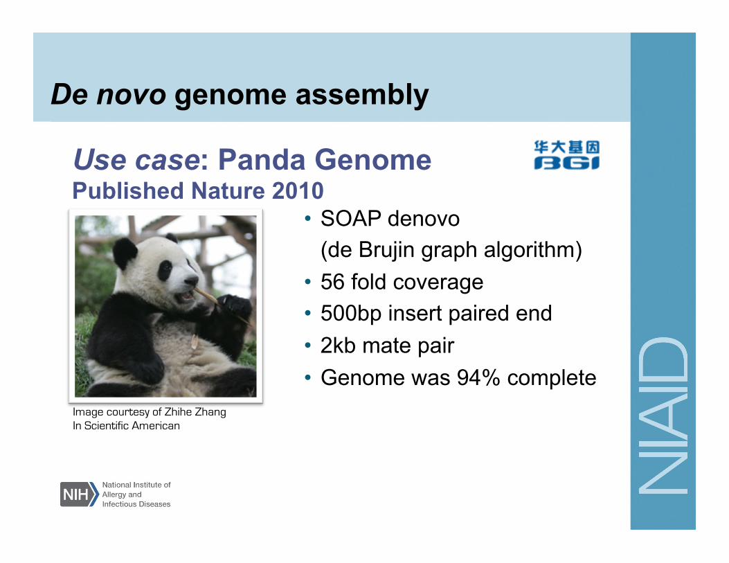
Use case: Panda Genome Published Nature 2010
• SOAP denovo (de Brujin graph algorithm)
• 56 fold coverage • 500bp insert paired end • 2kb mate pair • Genome was 94% complete
Image courtesy of Zhihe Zhang In Scientific American
De novo genome assembly
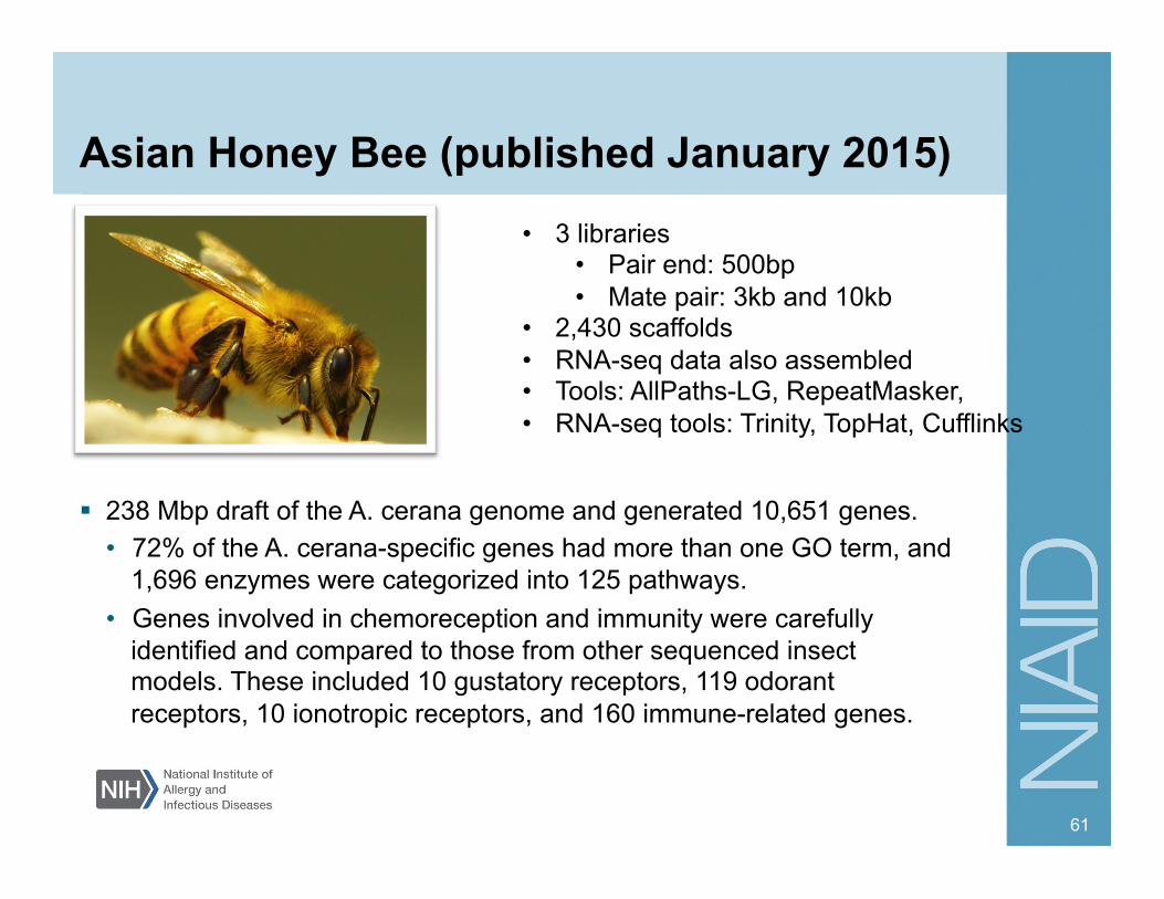
Asian Honey Bee (published January 2015)
238 Mbp draft of the A. cerana genome and generated 10,651 genes. • 72% of the A. cerana-specific genes had more than one GO term, and
1,696 enzymes were categorized into 125 pathways. • Genes involved in chemoreception and immunity were carefully
identified and compared to those from other sequenced insect models. These included 10 gustatory receptors, 119 odorant receptors, 10 ionotropic receptors, and 160 immune-related genes.
61
• 3 libraries • Pair end: 500bp • Mate pair: 3kb and 10kb
• 2,430 scaffolds • RNA-seq data also assembled • Tools: AllPaths-LG, RepeatMasker, • RNA-seq tools: Trinity, TopHat, Cufflinks
62
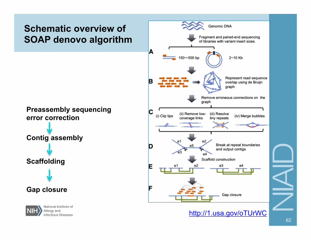
Schematic overview of SOAP denovo algorithm
http://1.usa.gov/oTUrWC
Contig assembly
Scaffolding
Preassembly sequencing error correction
Gap closure
RNA-Seq / miRNA-seq (noncoding, differential
expression, Novel splice forms,
antisense)
Epigenetics (Chip-Seq, Mnase-seq,
Bisulfite-Seq)
CNV, Structural variations
Targeted resequencing
“Exome analysis”
Whole genome sequencing
Metagenomics (16S microbiome,
environmental WGS)
Somatic mutations Variants in
mendelian diseases
High throughput sequencing
De novo genome
assembly
Beyond the basics – a growing list of NGS applications
64
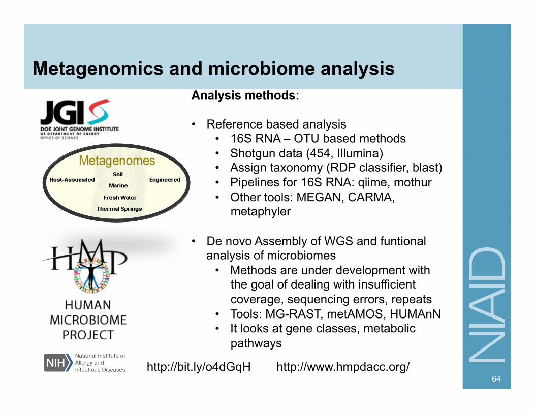
Metagenomics and microbiome analysis Analysis methods: • Reference based analysis
• 16S RNA – OTU based methods • Shotgun data (454, Illumina) • Assign taxonomy (RDP classifier, blast) • Pipelines for 16S RNA: qiime, mothur • Other tools: MEGAN, CARMA,
metaphyler
• De novo Assembly of WGS and funtional analysis of microbiomes
• Methods are under development with the goal of dealing with insufficient coverage, sequencing errors, repeats
• Tools: MG-RAST, metAMOS, HUMAnN • It looks at gene classes, metabolic
pathways
http://bit.ly/o4dGqH http://www.hmpdacc.org/
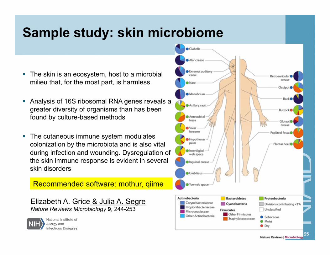
Sample study: skin microbiome
The skin is an ecosystem, host to a microbial milieu that, for the most part, is harmless.
Analysis of 16S ribosomal RNA genes reveals a greater diversity of organisms than has been found by culture-based methods
The cutaneous immune system modulates colonization by the microbiota and is also vital during infection and wounding. Dysregulation of the skin immune response is evident in several skin disorders
65
Elizabeth A. Grice & Julia A. Segre Nature Reviews Microbiology 9, 244-253
Recommended software: mothur, qiime
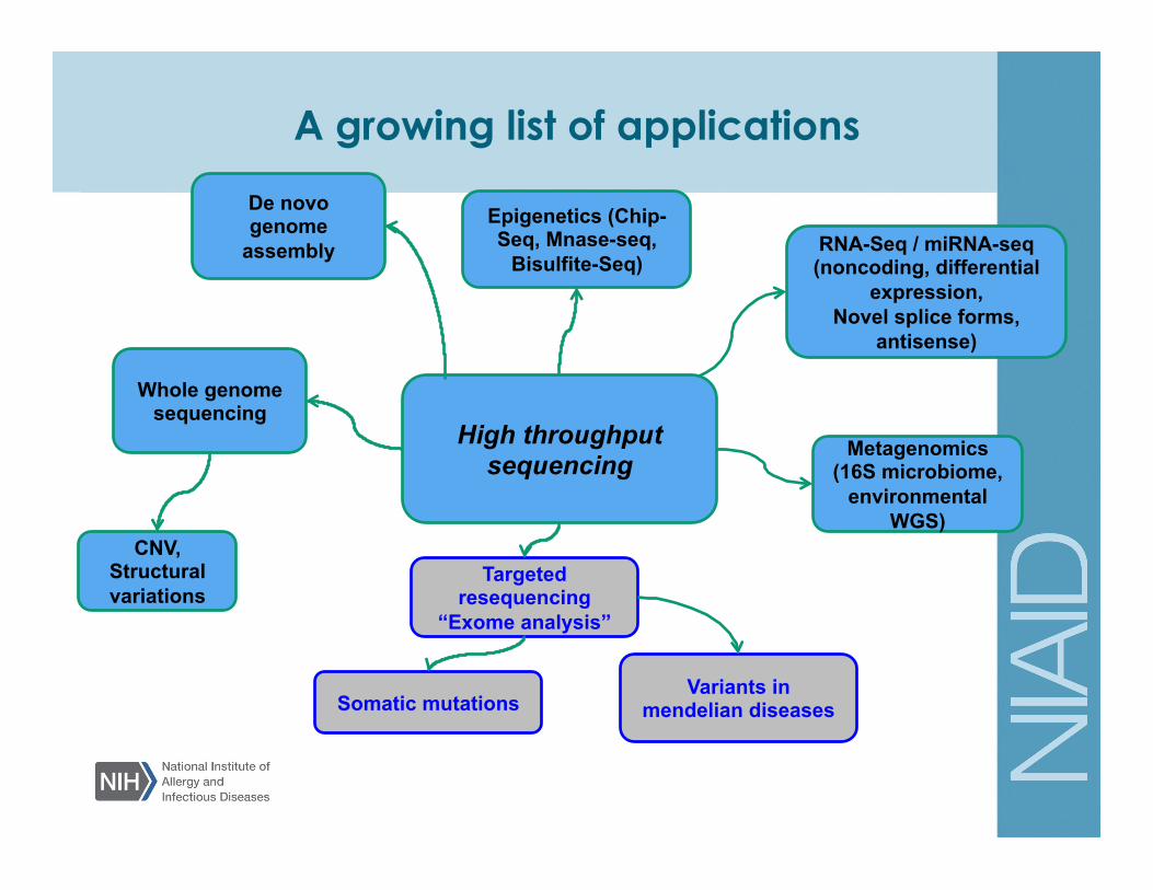
RNA-Seq / miRNA-seq (noncoding, differential
expression, Novel splice forms,
antisense)
Epigenetics (Chip-Seq, Mnase-seq,
Bisulfite-Seq)
CNV, Structural variations
Targeted resequencing
“Exome analysis”
Whole genome sequencing
Metagenomics (16S microbiome,
environmental WGS)
Somatic mutations Variants in
mendelian diseases
High throughput sequencing
De novo genome
assembly
A growing list of applications
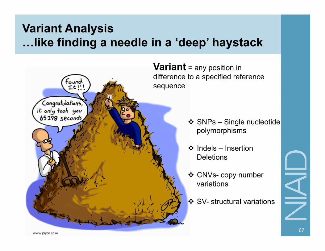
Variant Analysis …like finding a needle in a ‘deep’ haystack
67
SNPs – Single nucleotide polymorphisms
Indels – Insertion Deletions
CNVs- copy number variations
SV- structural variations
Variant = any position in difference to a specified reference sequence
68
Efforts at creating databases of variants:
HapMap Project • Project that started on 2002 with the goal of describing patterns of human
genetic variation and create a haplotype map using SNPs present in at least 1% of the population, which were deposited in dbSNPs.
• It used 269 individuals. Haplotypes – adjacent SNPs that are inherited together
1000 Genomes • Started in 2008 with a goal of using at least 1000 individuals (about
2,500 samples at 4X coverage), interrogate 1000 gene regions in 900 samples (exome analysis), find most genetic variants with allele frequencies above 1% and to a 0.1% if in coding regions as well as Indels and structural variants
• Make data available to the public ftp://ftp-trace.ncbi.nih.gov/1000genomes/ftp/ or via Amazon Cloud http://s3.amazonaws.com/1000genomes

Encode: Encyclopedia of DNA Elements
69
Main Goal: • Find all functional elements in the genome

Exome-Seq
Targeted exome capture targets ~20,000 variants
near coding sequences and a few rare missense or loss of function variants
Provides high depth of coverage for more accurate variant calling
It is starting to be used as a diagnostic tool
70
Ann Neurol. 2012 Jan;71(1):5-14.
-Nimblegen -Agilent -Illumina

VCF format (version 4.0)
71
Format used to report information about a position in the genome
Use by the 1000 genomes project to report all variants
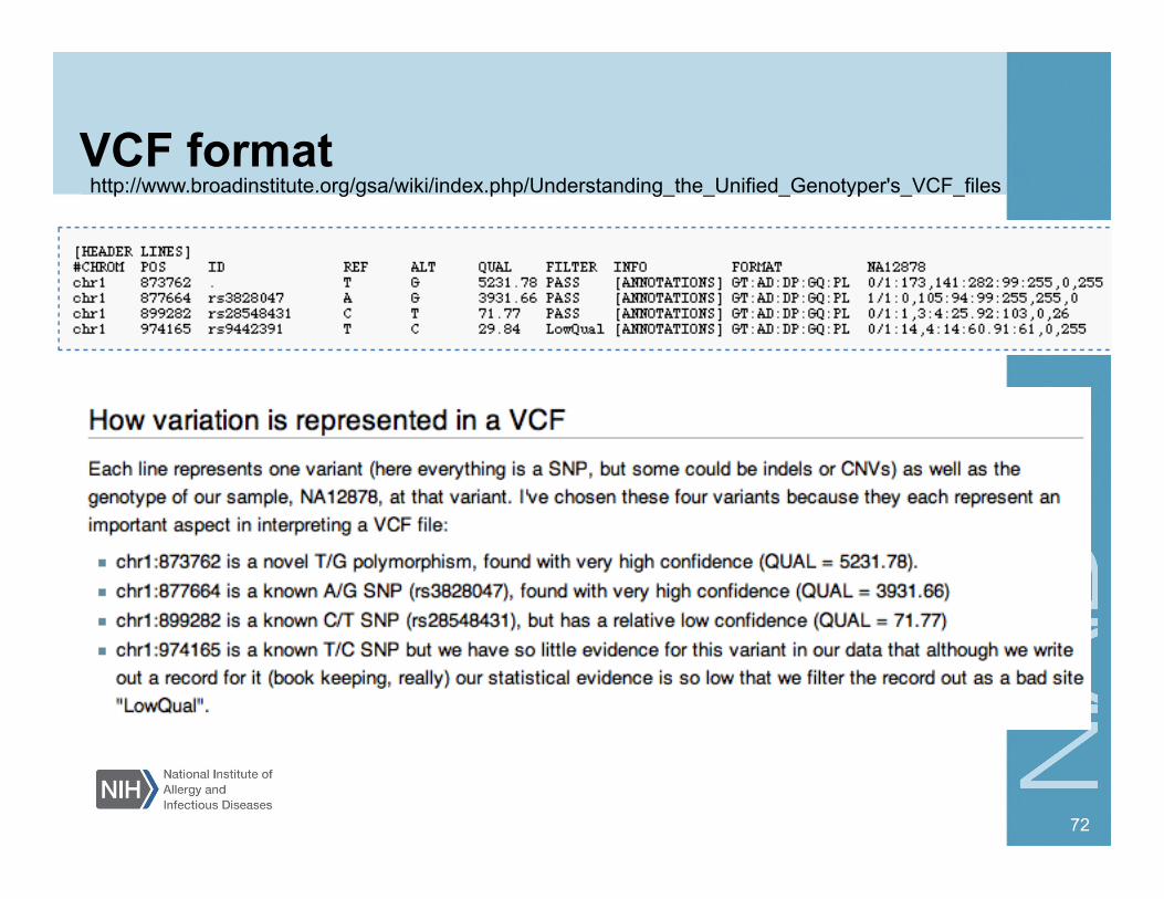
VCF format
72
http://www.broadinstitute.org/gsa/wiki/index.php/Understanding_the_Unified_Genotyper's_VCF_files