OVERVIEW OF BASIC AND

ADVANCED STATISTICAL

METHODS Professor Dr Noor Azina Ismail

Department of Applied Statistics

Faculty of Economics and Administration

University of Malaya

nazina@um.edu.my

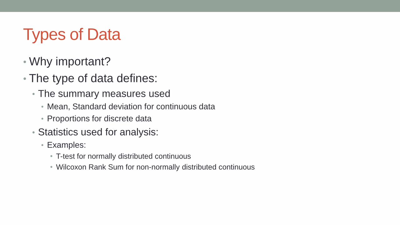
Types of Data

• Why important?

• The type of data defines:

• The summary measures used

• Mean, Standard deviation for continuous data

• Proportions for discrete data

• Statistics used for analysis:

• Examples:

• T-test for normally distributed continuous

• Wilcoxon Rank Sum for non-normally distributed continuous

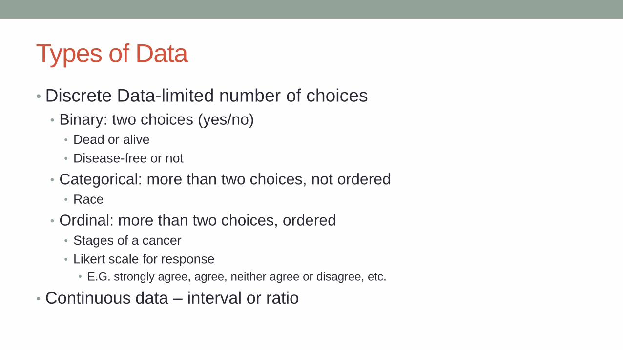
Types of Data

• Discrete Data-limited number of choices

• Binary: two choices (yes/no)

• Dead or alive

• Disease-free or not

• Categorical: more than two choices, not ordered

• Race

• Ordinal: more than two choices, ordered

• Stages of a cancer

• Likert scale for response

• E.G. strongly agree, agree, neither agree or disagree, etc.

• Continuous data – interval or ratio

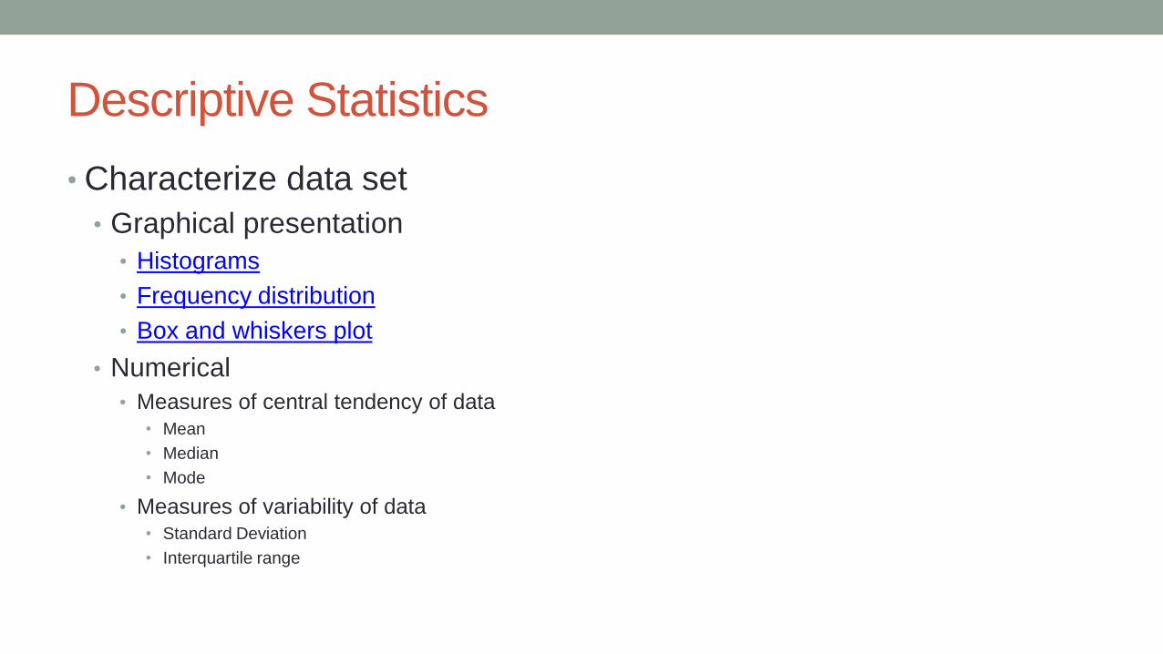
Descriptive Statistics

• Characterize data set

• Graphical presentation

• Histograms

• Frequency distribution

• Box and whiskers plot

• Numerical

• Measures of central tendency of data • Mean

• Median

• Mode

• Measures of variability of data • Standard Deviation

• Interquartile range

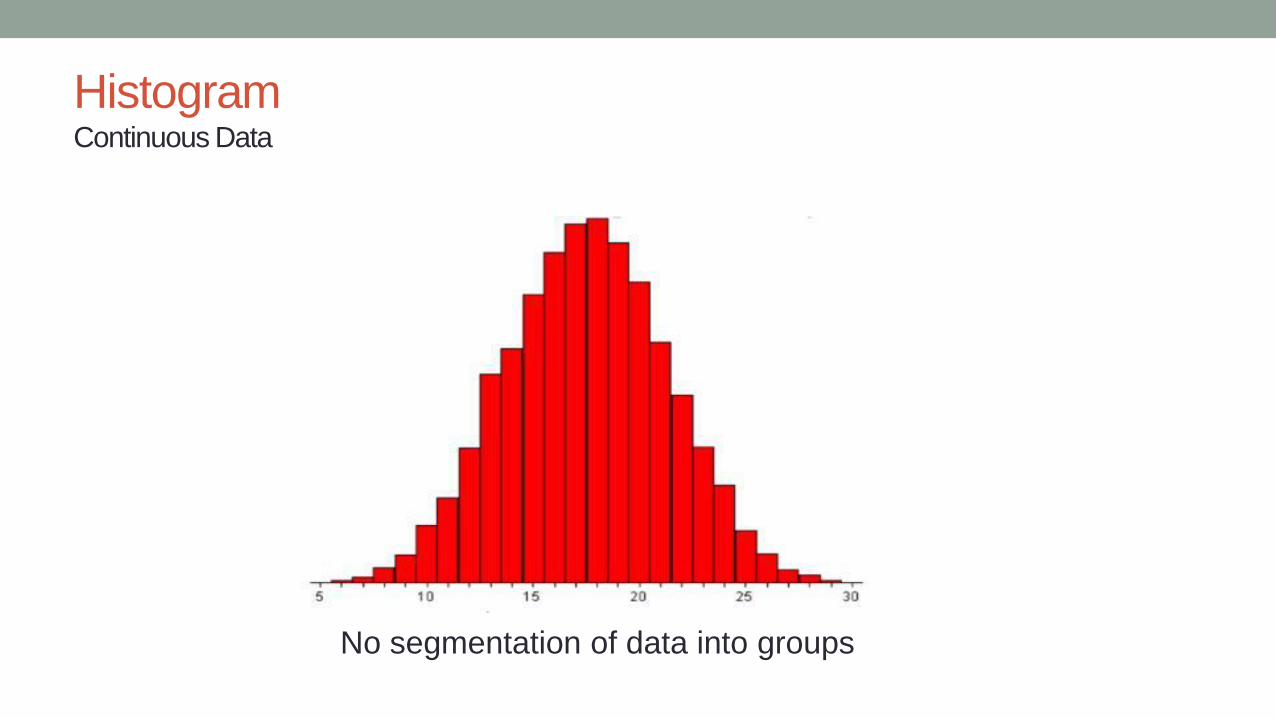
Histogram Continuous Data

No segmentation of data into groups

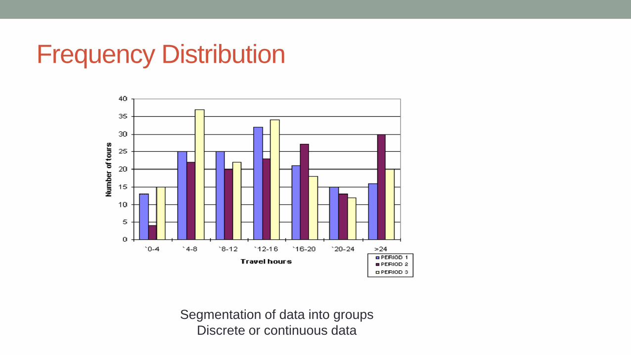
Frequency Distribution

Segmentation of data into groups

Discrete or continuous data

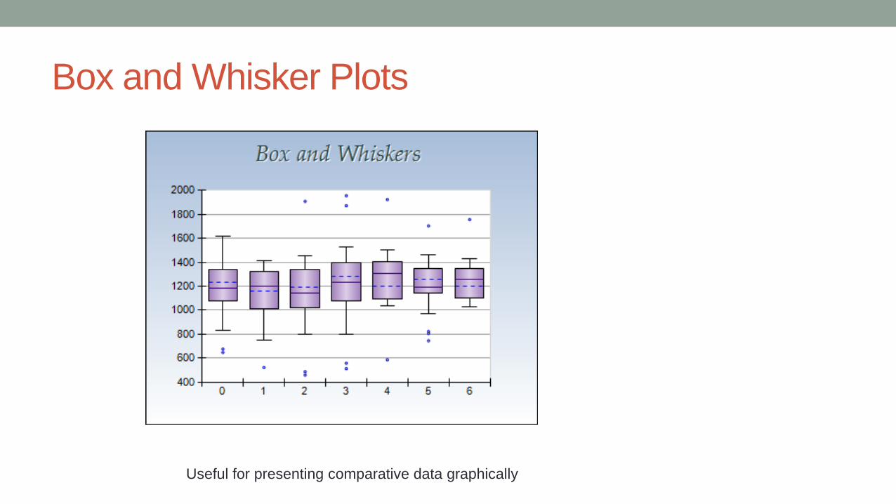
Box and Whisker Plots

Useful for presenting comparative data graphically

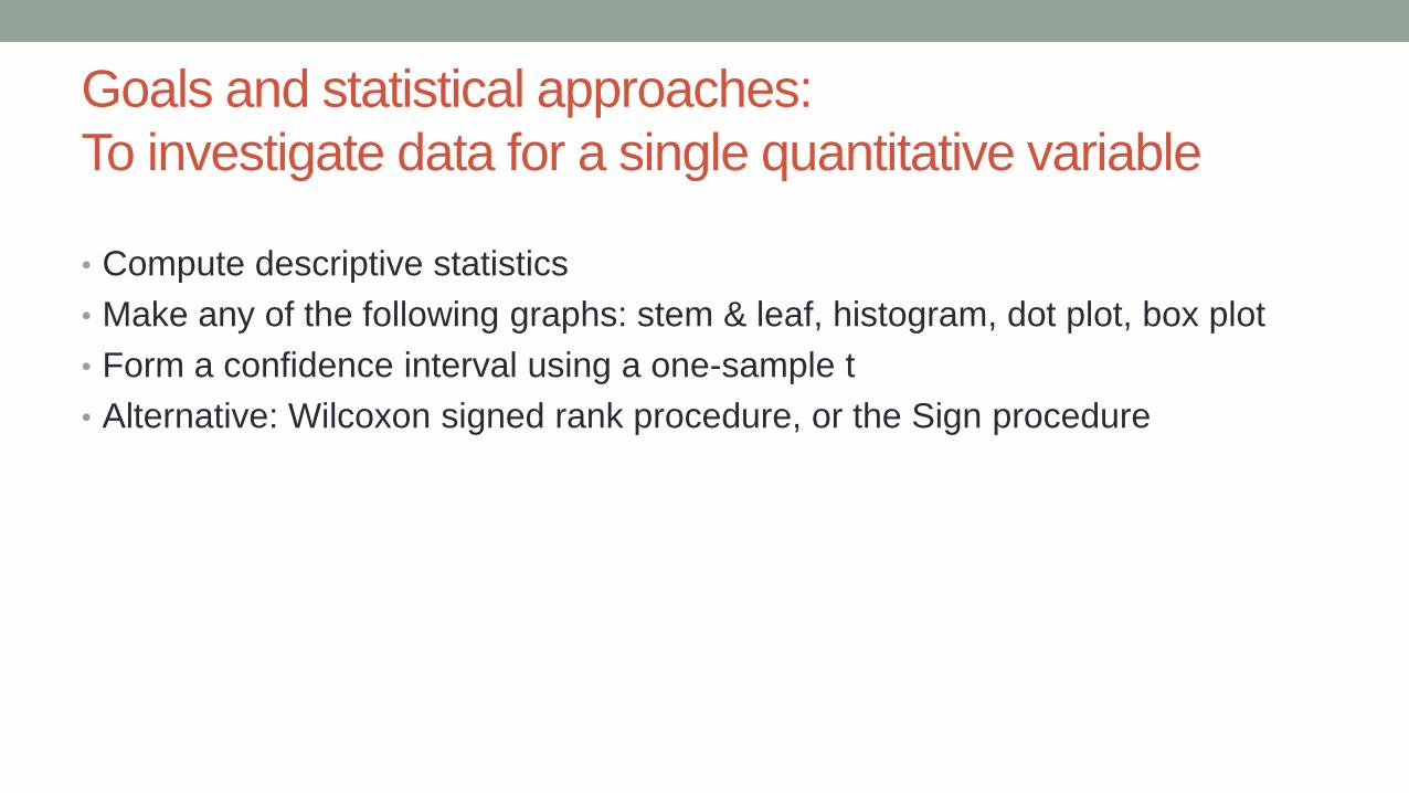
Goals and statistical approaches:

To investigate data for a single quantitative variable

• Compute descriptive statistics

• Make any of the following graphs: stem & leaf, histogram, dot plot, box plot

• Form a confidence interval using a one-sample t

• Alternative: Wilcoxon signed rank procedure, or the Sign procedure

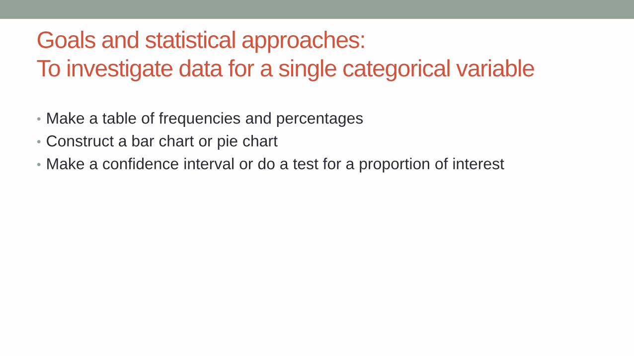
Goals and statistical approaches:

To investigate data for a single categorical variable

• Make a table of frequencies and percentages

• Construct a bar chart or pie chart

• Make a confidence interval or do a test for a proportion of interest

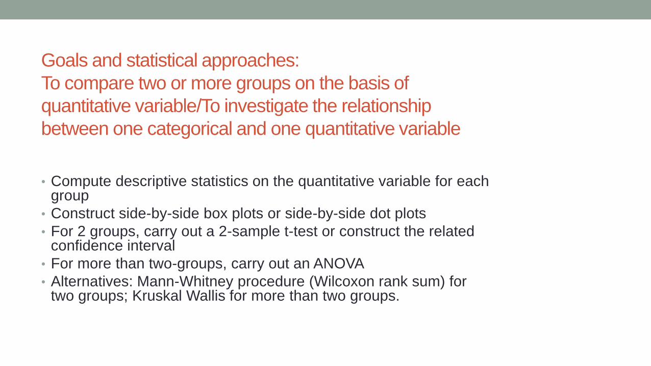
Goals and statistical approaches:

To compare two or more groups on the basis of

quantitative variable/To investigate the relationship

between one categorical and one quantitative variable

• Compute descriptive statistics on the quantitative variable for each group

• Construct side-by-side box plots or side-by-side dot plots

• For 2 groups, carry out a 2-sample t-test or construct the related confidence interval

• For more than two-groups, carry out an ANOVA

• Alternatives: Mann-Whitney procedure (Wilcoxon rank sum) for two groups; Kruskal Wallis for more than two groups.

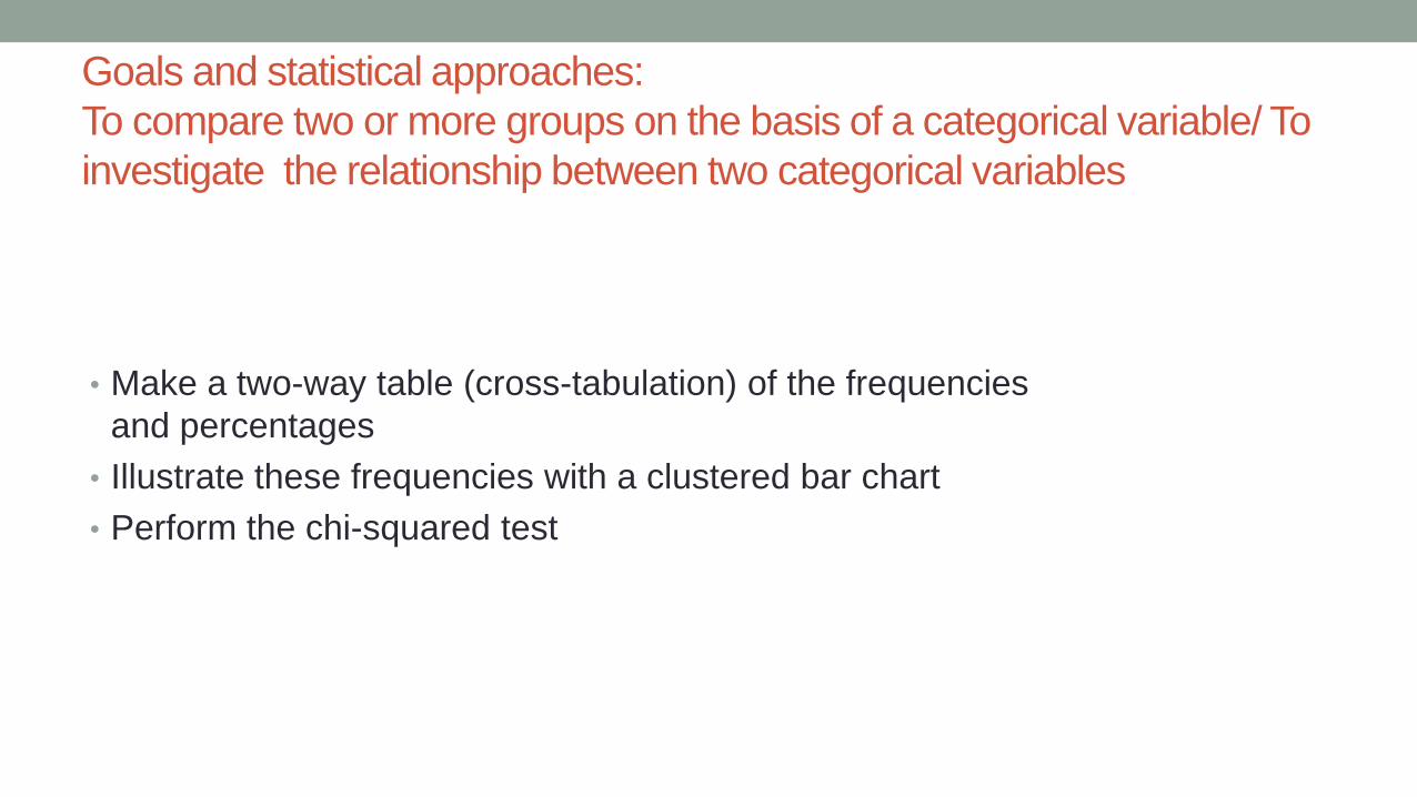
Goals and statistical approaches:

To compare two or more groups on the basis of a categorical variable/ To

investigate the relationship between two categorical variables

• Make a two-way table (cross-tabulation) of the frequencies

and percentages

• Illustrate these frequencies with a clustered bar chart

• Perform the chi-squared test

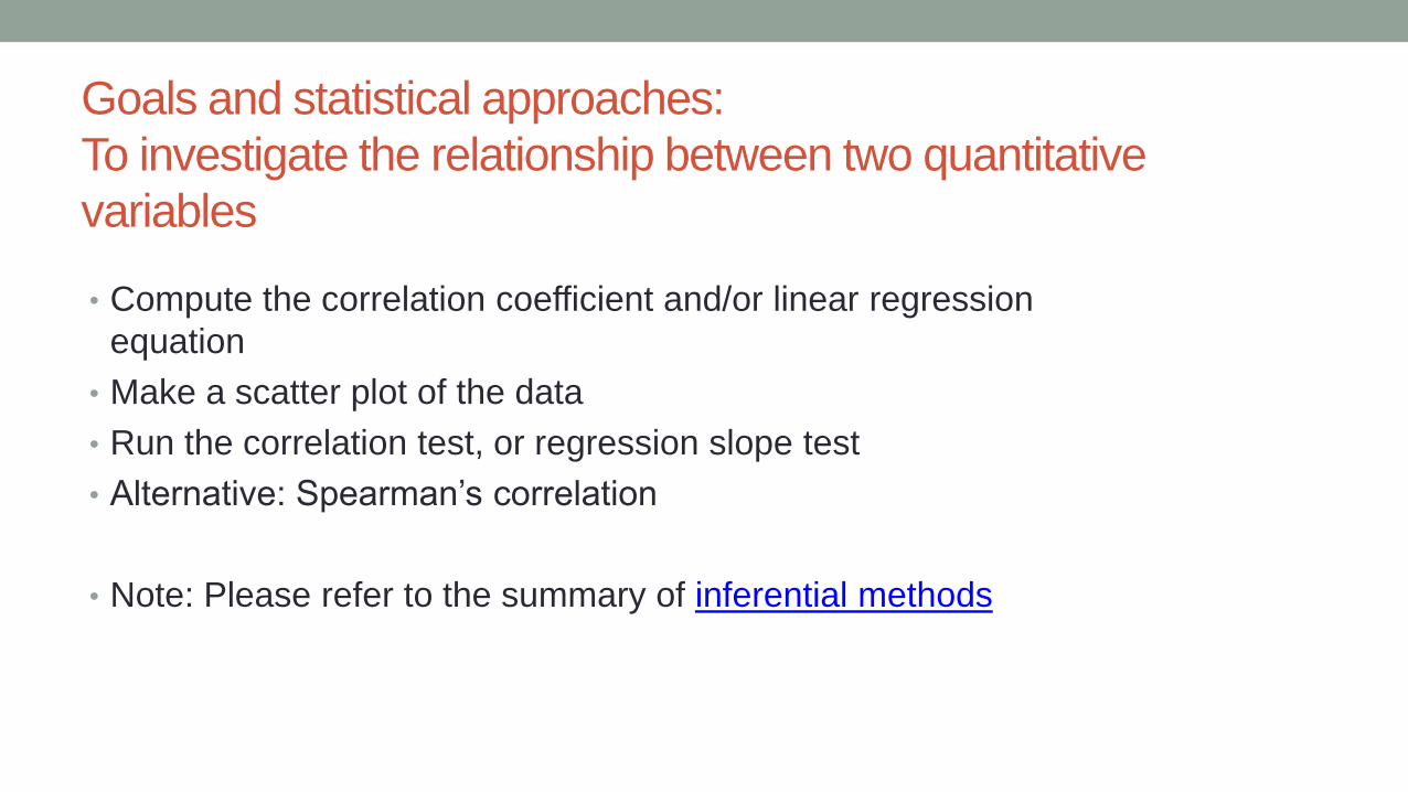
Goals and statistical approaches:

To investigate the relationship between two quantitative

variables

• Compute the correlation coefficient and/or linear regression

equation

• Make a scatter plot of the data

• Run the correlation test, or regression slope test

• Alternative: Spearman’s correlation

• Note: Please refer to the summary of inferential methods

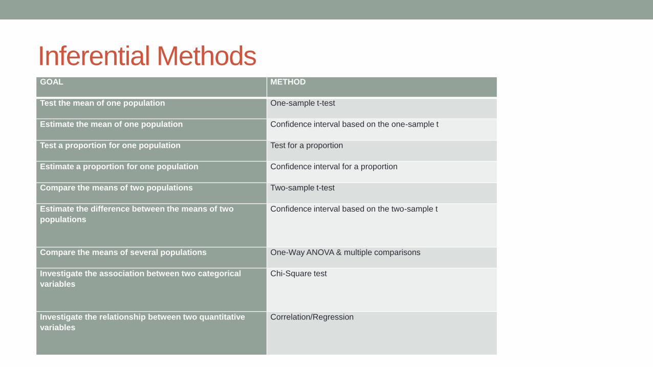
Inferential Methods GOAL METHOD

Test the mean of one population One-sample t-test

Estimate the mean of one population Confidence interval based on the one-sample t

Test a proportion for one population Test for a proportion

Estimate a proportion for one population Confidence interval for a proportion

Compare the means of two populations Two-sample t-test

Estimate the difference between the means of two

populations

Confidence interval based on the two-sample t

Compare the means of several populations One-Way ANOVA & multiple comparisons

Investigate the association between two categorical

variables

Chi-Square test

Investigate the relationship between two quantitative

variables

Correlation/Regression

Statistical Tests

• Parametric tests • Continuous data normally distributed

• Non-parametric tests • Continuous data not normally distributed

• Categorical or Ordinal data

• Most non-parametric tests are based on ranks or other non- value related methods

Regression

• Based on fitting a line to data • Provides a regression coefficient, which is the slope of the line

• Y = ax + b

• Use to predict a dependent variable’s value based on the value of an independent variable.

• Very helpful- In analysis of height and weight, for a known height, one can predict weight.

• Much more useful than correlation • Allows prediction of values of Y rather than just whether there is a relationship between two

variable.

Why Multivariate Analysis

• In published papers, the multivariable models are more

powerful than univariable models

• Theoretical reasons:

• Real-world is multidimensional and multicausal

• ie multiple IVs (predictors) and DVs (outcomes)

• Statistical reasons

• Examine large data sets in a single analysis

16

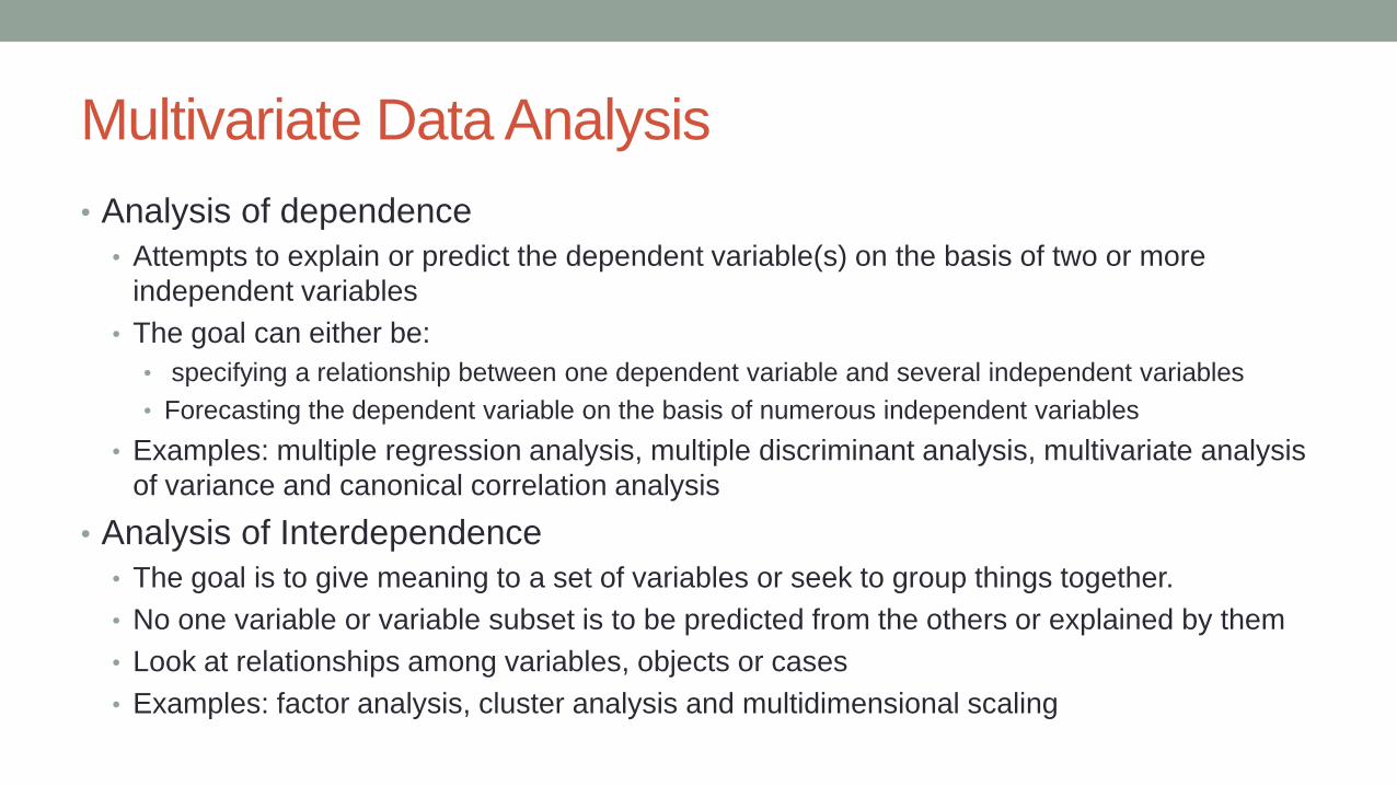
Multivariate Data Analysis

• Analysis of dependence

• Attempts to explain or predict the dependent variable(s) on the basis of two or more

independent variables

• The goal can either be:

• specifying a relationship between one dependent variable and several independent variables

• Forecasting the dependent variable on the basis of numerous independent variables

• Examples: multiple regression analysis, multiple discriminant analysis, multivariate analysis

of variance and canonical correlation analysis

• Analysis of Interdependence

• The goal is to give meaning to a set of variables or seek to group things together.

• No one variable or variable subset is to be predicted from the others or explained by them

• Look at relationships among variables, objects or cases

• Examples: factor analysis, cluster analysis and multidimensional scaling

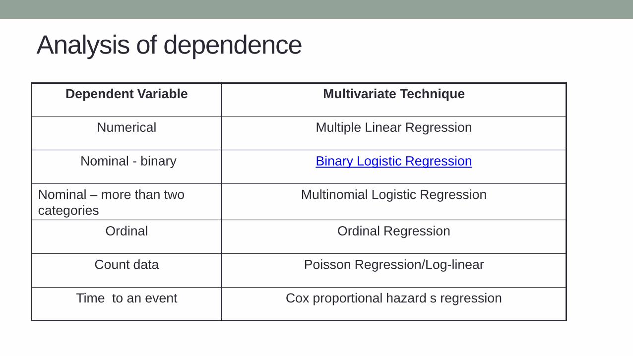
Analysis of dependence

Dependent Variable Multivariate Technique

Numerical Multiple Linear Regression

Nominal - binary Binary Logistic Regression

Nominal – more than two

categories

Multinomial Logistic Regression

Ordinal Ordinal Regression

Count data Poisson Regression/Log-linear

Time to an event Cox proportional hazard s regression

18

The Economics of Low Pay in Britain: A Logistic

Regression Approach (Sloane & Theodossiou, 1994) • One of the objectives is to identify the various personal and job characteristics

which cause an individual to be in a given income category especially the low

paid

• Here regressions are not used to identify causalities but to study the

probability of individuals being in the low earnings category.

• Low pay is defined as the first three deciles of the earnings distribution for all

workers. Middle pay is defined as the fourth to seventh deciles and high pay

as the eighth to tenth deciles

• Refer to the paper.

19

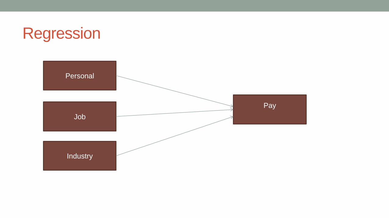
Regression

Personal

Job

Industry

Pay

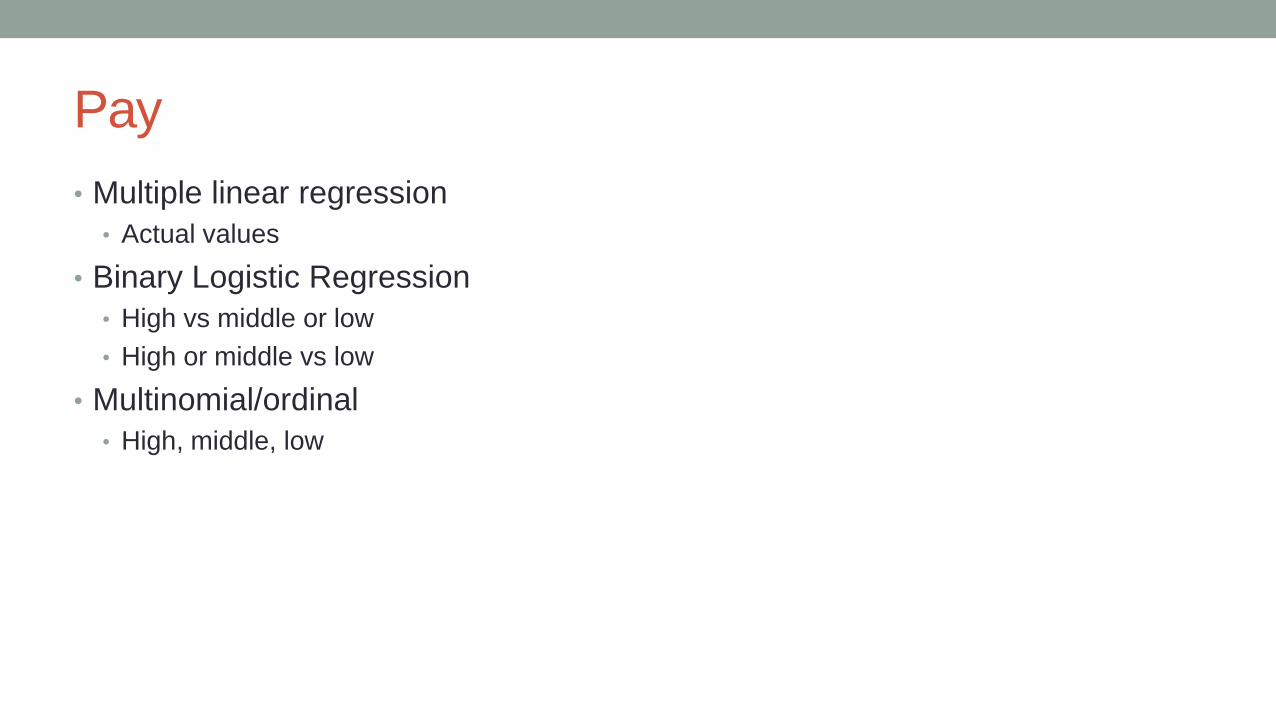
Pay

• Multiple linear regression

• Actual values

• Binary Logistic Regression

• High vs middle or low

• High or middle vs low

• Multinomial/ordinal

• High, middle, low

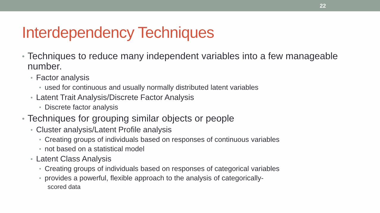
Interdependency Techniques

• Techniques to reduce many independent variables into a few manageable number. • Factor analysis

• used for continuous and usually normally distributed latent variables

• Latent Trait Analysis/Discrete Factor Analysis

• Discrete factor analysis

• Techniques for grouping similar objects or people • Cluster analysis/Latent Profile analysis

• Creating groups of individuals based on responses of continuous variables

• not based on a statistical model

• Latent Class Analysis

• Creating groups of individuals based on responses of categorical variables

• provides a powerful, flexible approach to the analysis of categorically-

scored data

22

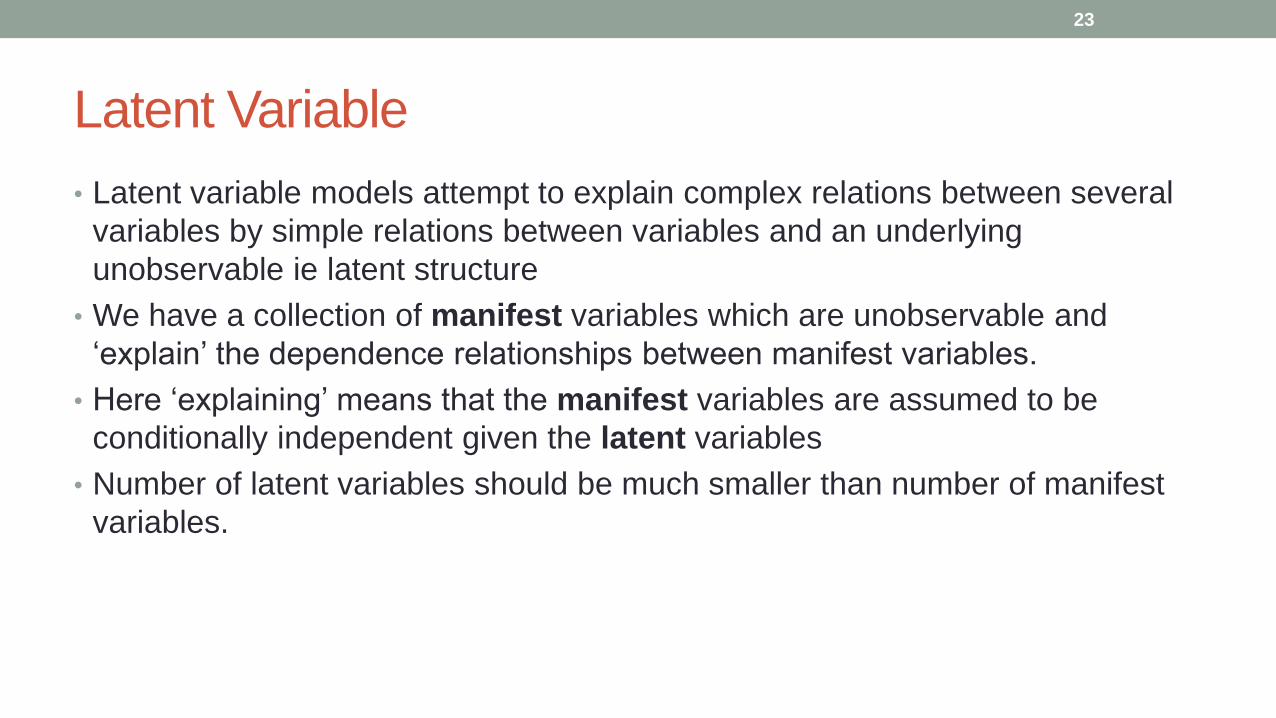
Latent Variable

• Latent variable models attempt to explain complex relations between several

variables by simple relations between variables and an underlying

unobservable ie latent structure

• We have a collection of manifest variables which are unobservable and

‘explain’ the dependence relationships between manifest variables.

• Here ‘explaining’ means that the manifest variables are assumed to be

conditionally independent given the latent variables

• Number of latent variables should be much smaller than number of manifest

variables.

23

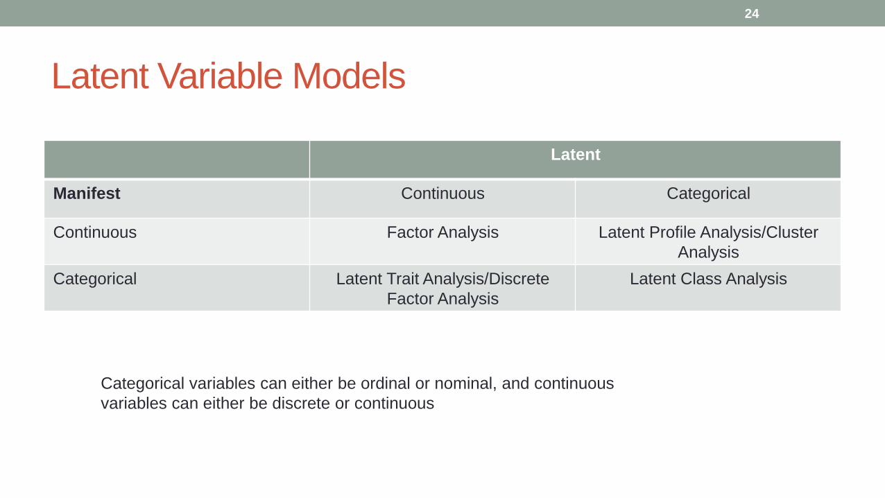
Latent Variable Models

Latent

Manifest Continuous Categorical

Continuous Factor Analysis Latent Profile Analysis/Cluster

Analysis

Categorical Latent Trait Analysis/Discrete

Factor Analysis

Latent Class Analysis

24

Categorical variables can either be ordinal or nominal, and continuous

variables can either be discrete or continuous

25

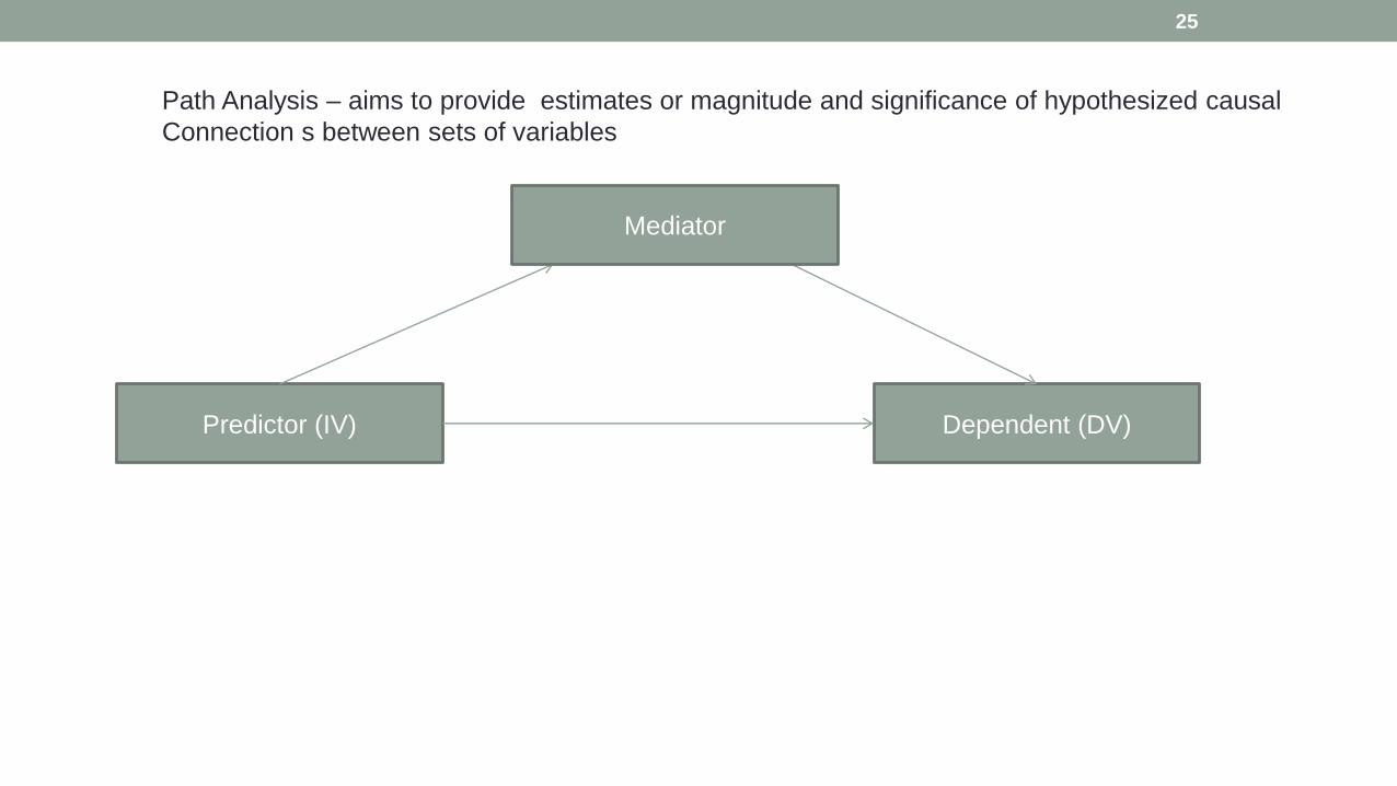
Predictor (IV) Dependent (DV)

Path Analysis – aims to provide estimates or magnitude and significance of hypothesized causal

Connection s between sets of variables

Mediator

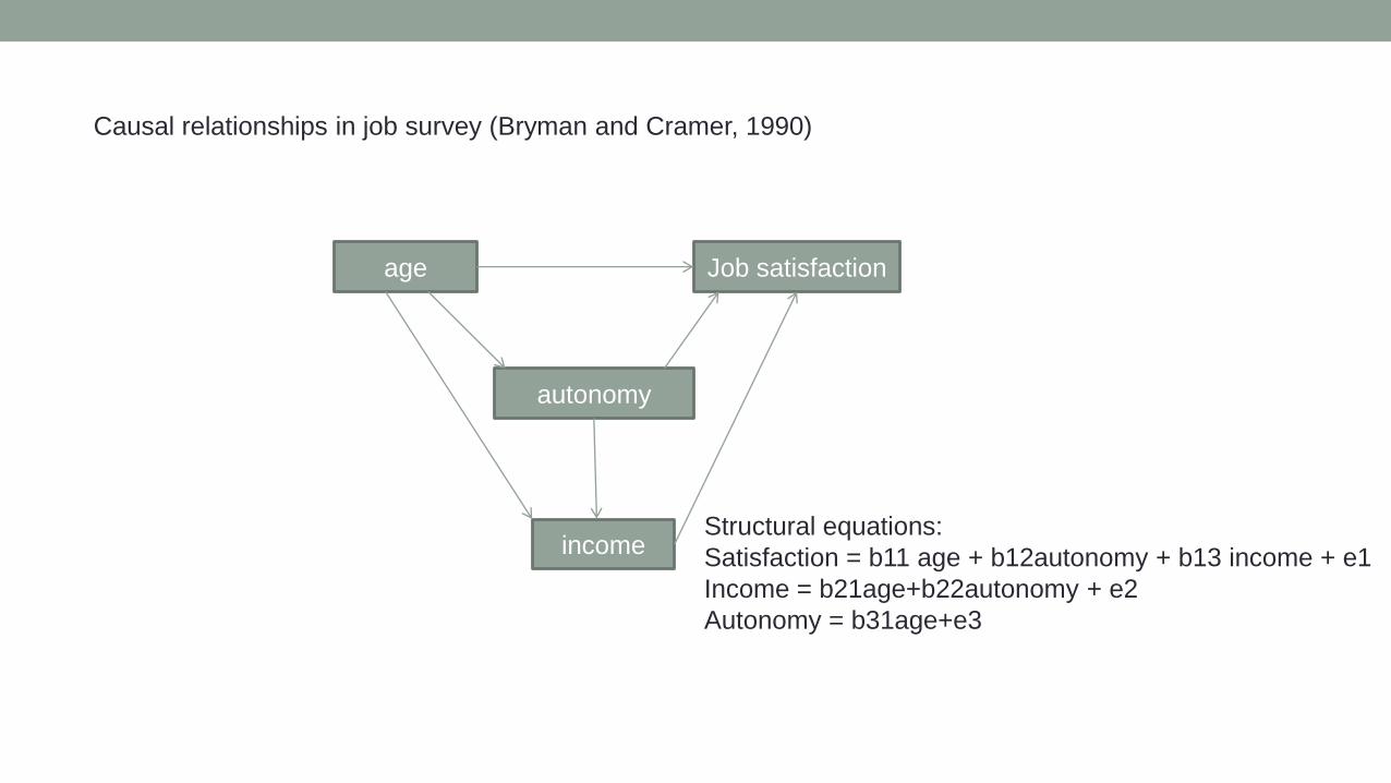
age Job satisfaction

autonomy

income

Causal relationships in job survey (Bryman and Cramer, 1990)

Structural equations:

Satisfaction = b11 age + b12autonomy + b13 income + e1

Income = b21age+b22autonomy + e2

Autonomy = b31age+e3

Structural Equation Modeling (SEM)

• SEM makes it possible to simultaneously estimate a measurement model, and to specify structural relations among the latent variables. The impressive flexibility of SEM allows the researcher to model data structures which violate traditional model assumptions such as heterogeneous error variances and correlated errors.

• Consists of • Measurement Model

• specifying relations between measured variables and underlying latent variables

• Structural Model

• specify structural relations among the latent variables

27

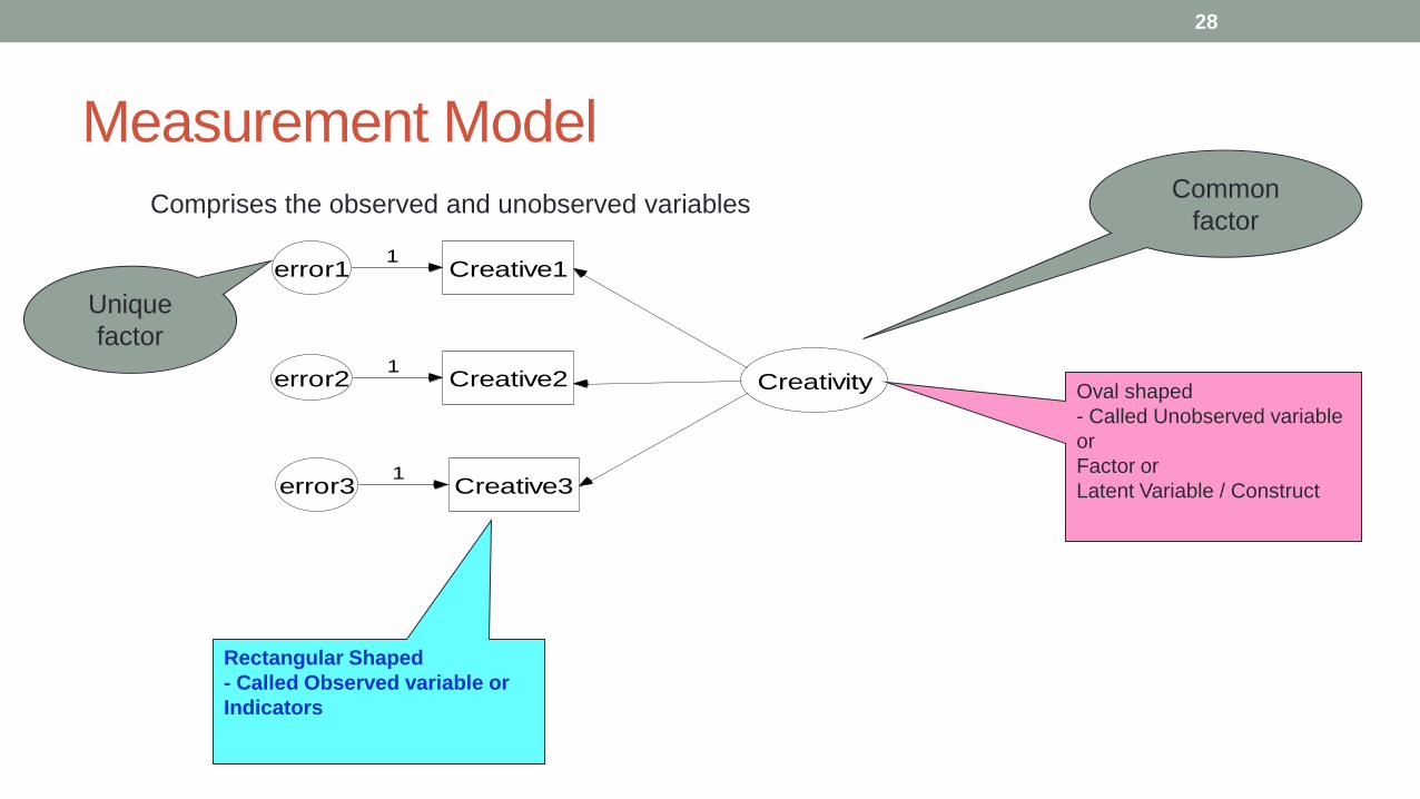
Measurement Model

28

Comprises the observed and unobserved variables

Creative1

Creative2

Creative3

Creativity

error11

error21

error31

Oval shaped

- Called Unobserved variable

or

Factor or

Latent Variable / Construct

Rectangular Shaped

- Called Observed variable or

Indicators

Common

factor

Unique

factor

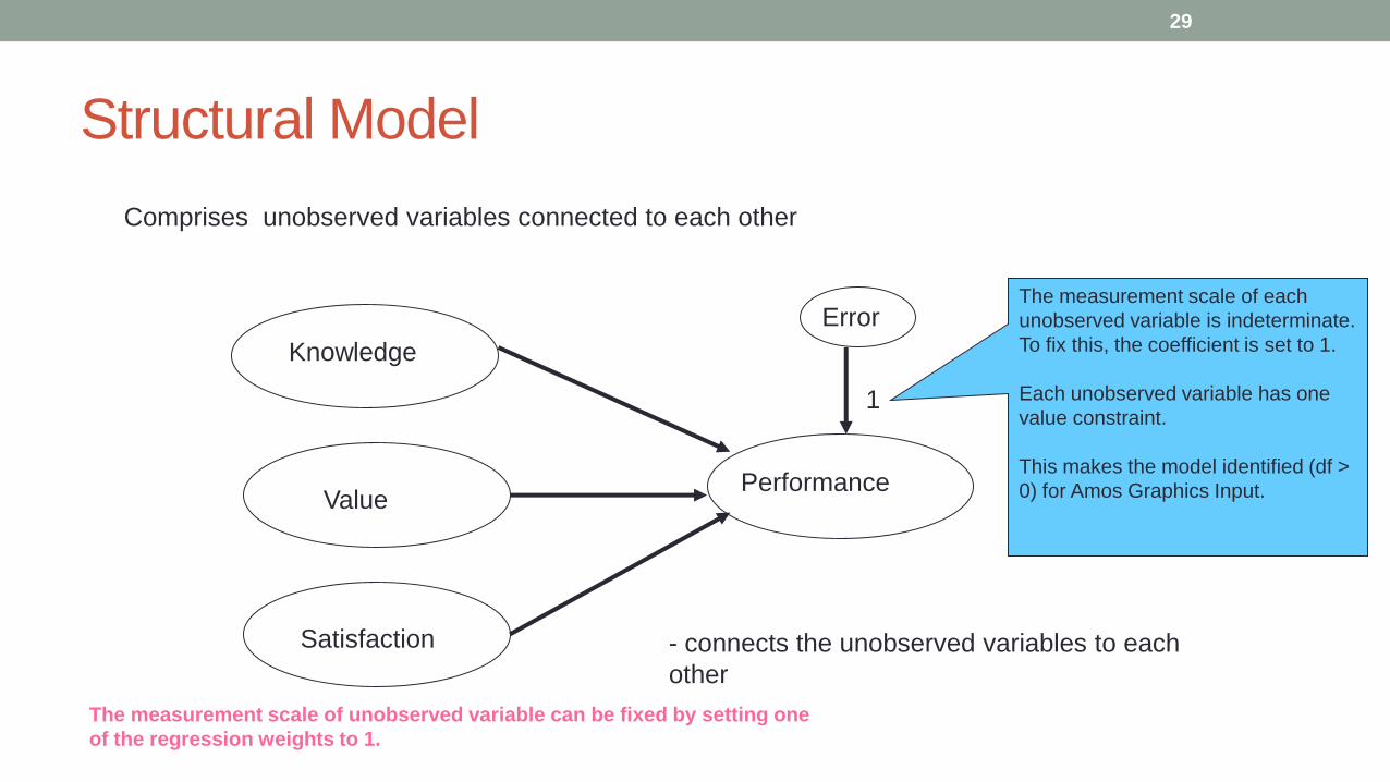
Structural Model

29

Comprises unobserved variables connected to each other

Knowledge

Value

Satisfaction

Performance

Error

1

- connects the unobserved variables to each

other

The measurement scale of each

unobserved variable is indeterminate.

To fix this, the coefficient is set to 1.

Each unobserved variable has one

value constraint.

This makes the model identified (df >

0) for Amos Graphics Input.

The measurement scale of unobserved variable can be fixed by setting one

of the regression weights to 1.

Nested Data Structure

• Hierarchical Modelling/Multilevel modelling

• account for nested data structure

• Observations are not independent of one another.

• Example : students nested in schools, children nested in families or

employees nested in companies

• Repeated observations nested within groups

• Individuals nested within groups

• Groups nested within communities

• Communities nested within cultures

30

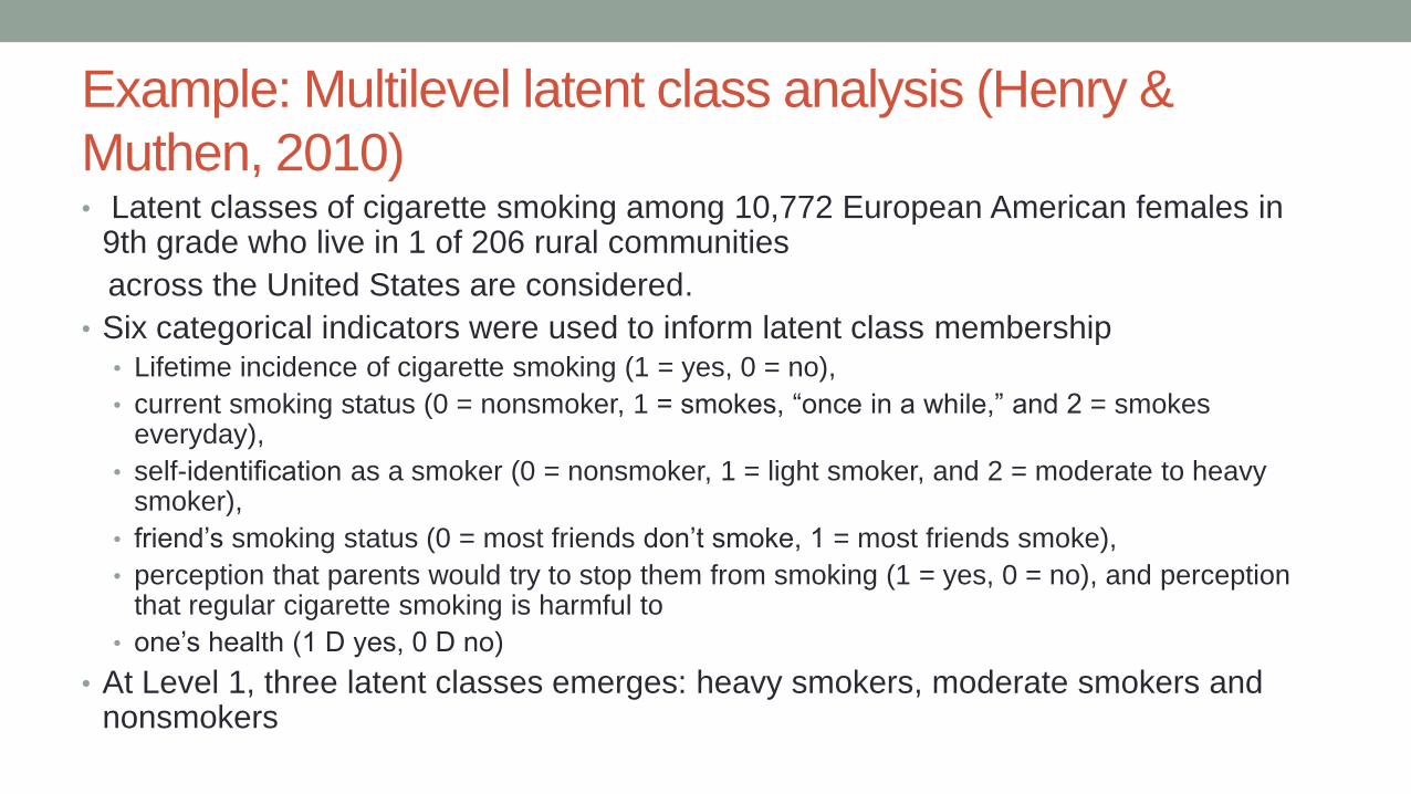
Example: Multilevel latent class analysis (Henry &

Muthen, 2010) • Latent classes of cigarette smoking among 10,772 European American females in

9th grade who live in 1 of 206 rural communities

across the United States are considered.

• Six categorical indicators were used to inform latent class membership

• Lifetime incidence of cigarette smoking (1 = yes, 0 = no),

• current smoking status (0 = nonsmoker, 1 = smokes, “once in a while,” and 2 = smokes everyday),

• self-identification as a smoker (0 = nonsmoker, 1 = light smoker, and 2 = moderate to heavy smoker),

• friend’s smoking status (0 = most friends don’t smoke, 1 = most friends smoke),

• perception that parents would try to stop them from smoking (1 = yes, 0 = no), and perception that regular cigarette smoking is harmful to

• one’s health (1 D yes, 0 D no)

• At Level 1, three latent classes emerges: heavy smokers, moderate smokers and nonsmokers

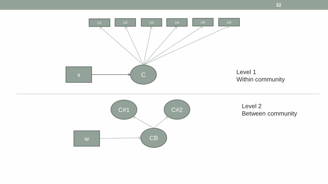
U1 U2 U3 U4 U5 U6

C x Level 1

Within community

C#1 C#2 Level 2

Between community

CB w

32