oscillator quantic mecanic

7/26/2019 oscillator quantic mecanic

http://slidepdf.com/reader/full/oscillator-quantic-mecanic 1/13

a r X i v : 1 1 0 4

. 2 5 9 1 v 1

[ m a t h - p h ] 1 3 A p r 2 0 1 1

CUQM - 139

Study of the generalized quantum isotonic nonlinear oscillator potential

Nasser Saad,1, ∗ Richard L. Hall,2, † Hakan Ciftci,3, ‡ and Ozlem Yesiltas3, §

1Department of Mathematics and Statistics, University of Prince Edward Island,550 University Avenue, Charlottetown, PEI, Canada C1A 4P3

2 Department of Mathematics and Statistics, Concordia University,

1455 de Maisonneuve Boulevard West, Montreal, Quebec, Canada H3G 1M8 3 Department of Physics, Faculty of Arts and Sciences, Gazi University, 06500 Ankara, Turkey.

We study the generalized quantum isotonic oscillator Hamiltonian given by H = −d2/dr2 + l(l +1)/r2 + w2r2 + 2g(r2 − a2)/(r2 + a2)2, g > 0. Two approaches are explored. A method for findingthe quasi-polynomial solutions is presented, and explicit expressions for these polynomials are given,along with the conditions on the potential parameters. By using the asymptotic iteration methodwe show how the eigenvalues of this Hamiltonian for arbitrary values of the parameters g, w and amay be found to high accuracy.

keyword: Non-linear oscillators; Non-polynomial potentials; Gol’dman and Krivchenkov potential; AsymptoticIteration Method; Quantum integrable systems; Laguerre polynomials.

PACS: 03.65.w, 03.65.Fd, 03.65.Ge.

I. INTRODUCTION

Recently, Carinena et al. [1] studied a quantum nonlinear oscillator potential whose Schrodinger equation reads− d2

dx2 + x2 + 8

2x2 − 1

(2x2 + 1)2

ψn(x) = E nψ(x) (1)

The interest in this problem came from the fact that it is exactly solvable, in a sense that the exact eigenenergies andeigenfunctions can be obtained explicitly. Indeed, Carinena et al. [1] were able to show that

ψn(x) =

P n(x)(2x2+1)e−x2/2,

E n = −3 + 2n, n = 0, 3, 4, 5, . . .

(2)

where the polynomials factors P n(x) are related to the Hermite polynomials by means of

P n(x) =

1 if n = 0H n(x) + 4nH n−2(x) + 4n(n − 3)H n−4(x) if n = 3, 4, 5, . . .

(3)

In a more recent work, Fellows and Smith [6] showed that the potential V (x) = x2 +8(2x2 − 1)/(2x2 + 1)2 as well as,for certain values of the parameters w, g and a, the potential V (x) = w2x2+2g(x2 − a2)/(x2 + a2)2 of the Schrodingerequation

− d2

dx2 + w2x2 + 2g

x2 − a2

(x2 + a2)2

ψn(x) = 2E nψ(x), (4)

are indeed supersymmetric partners of the harmonic oscillator potential. Using the supersymmetric approach, theauthors were able to construct an infinite set of exact soluble potentials, along with their eigenfunctions and eigen-values. Very recently, Sesma [9], using a Mobius transformation, was able to transform Eq.(4) into a confluent Heunequation [8] and thereby obtain an efficient algorithm to solve the Schrodinger equation (4) numerically.

∗Electronic address: [email protected]†Electronic address: [email protected]‡Electronic address: [email protected]§Electronic address: [email protected]

http://arxiv.org/abs/1104.2591v1



































mailto:[email protected]











2

The purpose of the present work is to provide a detailed solution, by means of the quasi-polynomial solutions and theapplication of the asymptotic iteration method [2–5], for the Schrodinger equation

− d2

dr2 +

l(l + 1)

r2 + w2r2 + 2g

r2 − a2

(r2 + a2)2

ψ(r) = 2Eψ(r), (5)

where l is the angular momentum number l = −1, 0, 1, . . . . Our results show that the quasi-exact solutions of Sesma[9] as well the results of Carinena et al. [1] follow as special cases of our general approach. The present article isorganized as follows. In the next section, some preliminary analysis of the Schrodinger equation (5) is presented. Ageneral approach for finding polynomial solutions of Eq.(5), for certain values of parameters w and g, is presented,and is based on a recent work of Ciftci et al. [3] for solving the second-order linear differential equation

3i=0

a3,ixi

y′′ +

2i=0

a2,ixi

y′ −

1i=0

τ 1,ixi

y = 0. (6)

More general quasi-exact solutions, including the results of Sesma [9], are discussed in section III. Unrestrictedsolutions of Eq.(5) based on the asymptotic iteration method are discussed in Section IV.

II. GENERALIZED QUANTUM ISOTONIC OSCILLATOR - PRELIMINARY RESULTS

A simple scaling argument, using r = a

2

x, allows us to write the equation (5) as− d2

dx2 +

l(l + 1)

x2 + (wa2)2x2 + 2g

x2 − 1

(x2 + 1)2

ψ(x) = 2Ea2ψ(x). (7)

A further substitution z = x2 + 1 yields a differential equation with two regular singular points at z = 0, 1 and oneirregular singular point of rank 2 at z = ∞. The roots µ’s of the indicial equation for the regular singular point z = 0reads µ± = 1

2(1 ± √ 1 + 4g), while the roots of the indicial equation at z = 1 are µ+ = (l + 1)/2 and µ− = −l/2.

Since the singularity for z → ∞ corresponds to that for x → ∞, it is necessary that the solution for z → ∞ behaveas ψ(x) ∼ exp(−wa2x2/2). Consequently, we may assume the general solution of equation (7) which vanishes at theorigin and at infinity takes the form

ψn(x) = xl+1(x2 + 1)µe−wa2

2 x2f n(x). (8)

A straightforward calculation shows that f n(x) are the solutions of the second-order homogeneous linear differentialequation

f ′′(x) +

2(l + 1)

x +

4µx

x2 + 1 − 2wa2x

f ′(x)

+

2Ea2 − wa2(2l + 3 + 4µ) +

2µ(2l + 3 + 2wa2) + 4µ(µ − 1) − 2g

x2 + 1 +

4(g − µ(µ − 1))

(x2 + 1)2

f (x) = 0. (9)

In the next sections, we attempt to give a general solution of this equation. For now, we assume that µ takes thevalue of the indicial root

µ ≡ µ− = 1

2(1 −

1 + 4g) (10)

which allows us to write Eq.(9) as

f ′′n(x) +

2(l + 1)

x +

4µx

x2 + 1 − 2wa2x

f ′n(x) +

2Ea2 − wa2(2l + 3 + 4µ) +

2µ(2l + 3 + 2wa2) + 2µ(µ − 1)

x2 + 1

f n(x) = 0.

(11)

We now consider the cases where the following two equations are satisfied

2µ(2l + 3 + 2wa2) + 2µ(µ − 1) = 0,

g = µ(µ − 1).



3

The solutions of this system, for g and µ, are given explicitly by

g = 0,

µ = 0,or

g = 2(1 + l + a2w)(3 + 2l + 2a2w),

µ = −2(1 + l + a2w).(12)

In the next, we consider each case of these two sets of solutions.

A. Case 1

The first set of solutions (g, µ) = (0, 0) reduces the differential equation (9) to

xf ′′n(x) + [−2wa2x2 + 2(l + 1)]f ′n(x) + (2Ea2 − wa2(2l + 3)) x f n(x) = 0 (13)

which is a special case of the general differential equation

(a3,0x3 + a3,1x2 + a3,2x + a3,3) y ′′ + (a2,0x2 + a2,1x + a2,2) y ′ − (τ 1,0x + τ 1,1) y = 0, (14)

with a3,0 = a3,1 = a3,3 = a2,1 = τ 1,1 = 0, a3,2 = 1, a2,0 = −2wa2, a2,2 = 2(l + 1), and τ 1,0 = −2Ea2 + wa2(2l + 3).The necessary and sufficient conditions for polynomial solutions of Eq.(14) are given by the following theorem [3].

Theorem 1. The second-order linear differential equation ( 14) has a polynomial solution of degree n if

τ 1,0 = n(n − 1)a3,0 + na2,0, n = 0, 1, 2, . . . , (15)

along with the vanishing of (n + 1) × (n + 1)-determinant ∆n+1 given by

∆n+1 =

β 0 α1 η1γ 1 β 1 α2 η2

γ 2 β 2 α3 η3. . .

. . . . . .

. . .γ n−2 β n−2 αn−1 ηn−1

γ n−1 β n−1 αn

γ n β n

= 0

where

β n = τ 1,1 − n((n − 1)a3,1 + a2,1)

αn = −n((n − 1)a3,2 + a2,2)

γ n = τ 1,0 − (n − 1)((n − 2)a3,0 + a2,0)

ηn = −n(n + 1)a3,3 (16)

and τ 1,0 is fixed for a given n in the determinant ∆n+1 = 0.

Thus, the necessary condition for the differential equation (13) to have polynomial solutions f n(x) =n

i=0 cixi is

2E na2 = wa2(2n′ + 2l + 3), n′ = 0, 1, 2, . . . (17)

while the sufficient condition, Eq(16), is

∆n+1 =

0 α1 0 0γ 1 0 α2 0

γ 2 0 α3 0. . .

. . . . . .

. . .γ n−2 0 αn−1 0

γ n−1 0 αn

γ n 0

=

0 if n = 0, 2, 4, . . .

n−1

2j=0

(−1)2j+1α2j+1γ 2j+1 = 0 if n = 1, 3, 5, . . .



4

where β n = 0, αn = −n(n + 2l + 1) and γ n = 2wa2(n − n′ − 1).

If l = −1, the determinant ∆n+1 is identically zero for all n, which is equivalent to the exact solutions of theone-dimensional harmonic oscillator problem.

For l = −1, we have for n = 0, 2, 4, . . . , ∆n+1 ≡ 0 and we obtain the exact solutions of the Gol’dman and Krivchenkov(or Isotonic) Hamiltonian H 0 where

H 0ψnl(x)

≡ − d2

dx2

+ l(l + 1)

x2

+ w2a4x2ψnl(x) = 2E g=0nl a2ψnl(x), 0

≤x <

∞. (18)

These exact solutions are given by [7]

2a2E g=0nl = wa2(4n + 2l + 3), n = 0, 1, 2, . . .

ψnl(x) = xl+1e−wa2x2/21F 1(−n; l + 3

2 ; wa2x2), n = 0, 1, 2, . . . .

(19)

where the confluent hypergeometric function 1F 1(−n; a; z) defined, in terms of the Pochhammer symbol (or Gammafunction Γ(a))

(a)k = Γ(a + k)

Γ(a) =

1 if (k = 0, a ∈ C\{0})a(a + 1)(a + 2) . . . (a + k − 1) if (k = N, a ∈ C)

as

1F 1(−n; a; z) =

nk=0

(

−n)kzk

(a)kk! . (20)

The polynomial solutions f n(x) = 1F 1(−n; l + 32 ; wa2x2) are easily obtained by using the asymptotic iteration method

(AIM), which is summarized by means of the following theorem.

Theorem 2: (H. Ciftci et al.[4], equations (2.13)-(2.14)) Given λ0 ≡ λ0(x) and s0 ≡ s0(x) in C ∞, the differential equation

f ′′(x) = λ0(x)f ′(x) + s0(x)f (x)

has the general solution

f (x) = exp

−

x α(t)dt

C 2 + C 1

x exp

t (λ0(τ ) + 2α(τ )) dτ

dt

(21)

if for some n ∈ N+ = {1, 2, . . .}snλn

= sn−1

λn−1= α(x), or δ n(x) = λnsn−1 − λn−1sn = 0, (22)

where

λn = λ′n−1 + sn−1 + λ0λn,

sn = s′n−1 + s0λn. (23)

For the differential equation (13) with

λ0(x) = − (−2wa2x2+2(l+1))x ,

s0(x) = −(2Ea2 − wa2(2l + 3),

(24)

the first few iterations with δ n = λnsn−1 − λn−1sn = 0, using (21), implies

f 0(x) = 1f 1(x) = 2wa2x2 − (2l + 3)f 2(x) = 4w2a4x4 − 4wa2(2l + 5)x2 + (2l + 3)(2l + 5). . .

(25)

which we may easily generalized using the definition of the confluent hypergeometric function, Eq(20), as

f n(x) = 1F 1(−n; l + 3

2; wa2x2) (26)

up to a constant.



5

B. Case 2

The second set of solutions

(g, µ) = (2(1 + l + a2w)(3 + 2l + 2a2w), −2(1 + l + a2w))

allow us to write the differential equation (9) as

f ′′n(x) +

2(l + 1)

x − 8(l + 1 + a2w)x

x2 + 1 − 2wa2x

f ′n(x) +

2Ea2 + wa2(6l + 5 + 8wa2)

f n(x) = 0. (27)

A further change of variable z = x2 + 1 allows us to write the differential equation (27) as

4z(z − 1)f ′′(z) − 4a2wz2 + 2(6l + 5 + 6wa2)z − 16(l + 1 + wa2)

f ′(z) + (2Ea2 + wa2(6l + 5 + 8wa2))z f (z) = 0,

(28)

Again, Eq.(28) is a special case of the differential equation ( 14) with a3,0 = a3,3 = τ 1,1 = 0, a3,1 = 4, a3,2 = −4, a2,0 =−4wa2, a2,1 = −2(6l + 5 + 6wa2), a2,2 = 16(l + 1 + wa2) and τ 1,0 = −2Ea2 − wa2(6l + 5 + 8wa2). Consequently, thepolynomial solutions f n(x) of (28) are subject to the following two conditions: the necessary condition (15) reads

2E na2 = wa2(4n′ − 6l − 5 − 8wa2), n′ = 0, 1, 2, . . . (29)

and the sufficient condition; namely, the vanishing of the tridiagonal determinant Eq(16), reads

∆n+1 =

β 0 α1

γ 1 β 1 α2

γ 2 β 2 α3

. . . . . .

. . .γ n−2 β n−2 αn−1


γ n β n

= 0

where

β n = −2n(2n − 6l − 7 − 6wa2)

αn = 4n(n

−4l

−5

−4a2w)

γ n = 4wa2(n − n′ − 1) (30)

and n′ = n is fixed for the given dimension of the determinant ∆n+1. From the sufficient condition (30) we obtainthe following conditions on the parameters

∆2 = 0 ⇒ a2w(l + 1 + a2w) = 0

∆3 = 0 ⇒ a2w(l + 1 + a2w)(1 + 2l + 2a2w) = 0

∆4 = 0 ⇒ a2w(l + 1 + a2w)(1 + 2l + 2a2w)(3(1 + 6l) + 14a2w) = 0

∆5 = 0 ⇒ a2w(l + 1 + a2w)(1 + 2l + 2a2w)(3(6l − 1)(6l + 1) + 4(38l + 1)a2w + 44a4w2) = 0

∆6 = 0 ⇒ a2w(l + 1 + a2w)(1 + 2l + 2a2w)(3(2l − 1)(6l − 1)(6l + 1) + 2(208l2 − 54l − 5)a2w + 200la4w2) = 0

. . . = . . .

For a physically meaningful solution we must have a2w > 0. This is possible for a very restricted value of the angularmomentum number l. Since β 0 = 0, we may observe that

∆n+1 =(l + 1 + a2w)(1+2l + 2a2w)×

β 2 α3

γ 3 β 3 α4

γ 4 β 4 α5

. . . . . .

. . .γ n−2 β n−2 αn−1


γ n β n

=(l + 1 + a2w)(1+2l + 2a2w) × Qln−1(a2w)



6

where Qln−1(a2w) are polynomials in the parameter product a2w.

For physically acceptable solutions, we must have l = −1 and the factor (l + 1 + a2w) yields a2w = 0, which is notphysically acceptable; so we ignore it. The second factor (1 + 2l + 2a2w) implies a special value of a2w = 1/2, for alln, which we will study shortly in full detail. Meanwhile, the polynomials Ql

n(a2w)

Ql=−1n−1 (a2w) =

1 if n = 214a2w − 15 if n = 344a4w2

−148a2w + 105 if n = 4

200a4w2 − 514a2w + 315 if n = 5. . .

(31)

give new values, not reported before, of a2w that yield quasi-exact solutions of the Schrodinger equation (with oneeigenstate)

−ψ′′n(x) +

(wa2)2x2 + 4a2w(1 + 2a2w)

(x2 − 1)

(x2 + 1)2

ψn(x) = wa2(4n + 1 − 8a2w)ψn(x) (32)

where

ψn(x) = (x2 + 1)−2a2we−wa2x2/2f n(x),

and f n(x) are the solutions of

4z(z − 1)f ′′

(z) − 4a

2

wz2

+ 2(−1 + 6wa2

)z − 16wa2

f ′

(z) + 4nwa2

z f (z) = 0, z = x2

+ 1. (33)

For example, ∆4 = 0 implies, using (31), that a2w = 1514 , and thus we have for

−ψ′′3 (x) +

225

196x2 +

660

49

(x2 − 1)

(x2 + 1)2

ψ3(x) =

465

98 ψ3(x), (34)

the exact solution

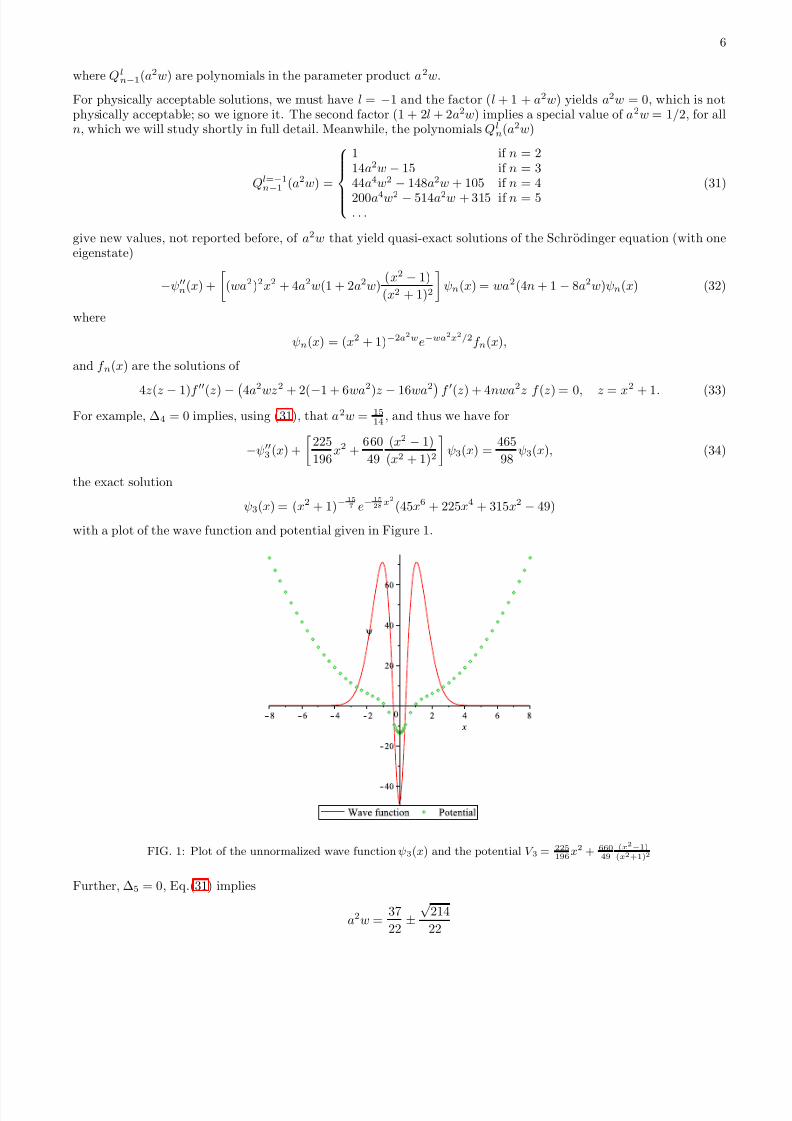
ψ3(x) = (x2 + 1)−157 e−

1528

x2(45x6 + 225x4 + 315x2 − 49)

with a plot of the wave function and potential given in Figure 1.

FIG. 1: Plot of the unnormalized wave function ψ3(x) and the potential V 3 = 225196

x2 + 66049

(x2−1)(x2+1)2

Further, ∆5 = 0, Eq.(31) implies

a2w = 37

22 ±

√ 214

22



7

and we have for

−ψ′′4 (x) +

(

37

22 ±

√ 214

22 )2x2 + 2(

37

11 ±

√ 214

11 )(

48

11 ±

√ 214

11 )

(x2 − 1)

(x2 + 1)2

ψ4(x) = (

37

22 ±

√ 214

22 )(

39

11 ∓ 4

√ 214

11 )ψ4(x)

(35)

the exact solutions

ψ

±

4 (x) = (x

2

+ 1)

−( 3711±√ 21411

)

e

−( 3744±√ 21444

)x2

(1575x8 + (9660 ± 420√

214)x6 + (26250 ± 2100√

214)x4 + (29820 ± 2940√

214)x2 − (1129 ± 188√

214)).

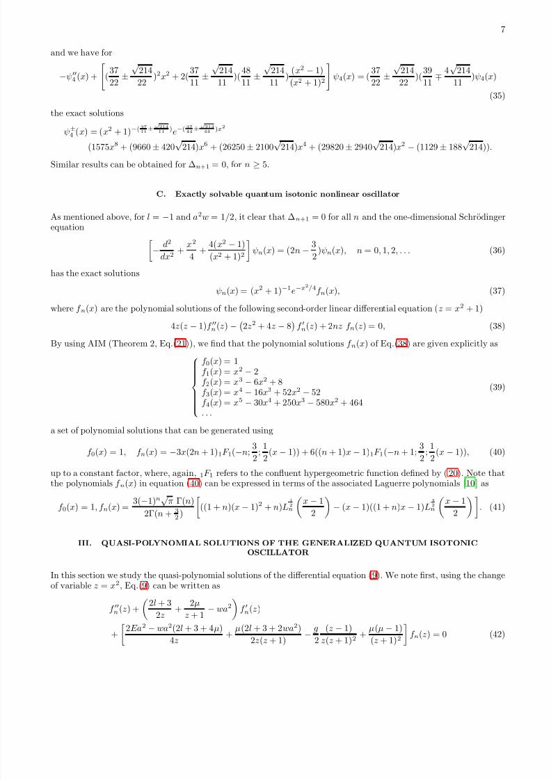
Similar results can be obtained for ∆n+1 = 0, for n ≥ 5.

C. Exactly solvable quantum isotonic nonlinear oscillator

As mentioned above, for l = −1 and a2w = 1/2, it clear that ∆n+1 = 0 for all n and the one-dimensional Schrodingerequation

− d2

dx2 +

x2

4 +

4(x2 − 1)

(x2 + 1)2

ψn(x) = (2n − 3

2)ψn(x), n = 0, 1, 2, . . . (36)

has the exact solutions

ψn(x) = (x2 + 1)−1e−x2/4f n(x), (37)

where f n(x) are the polynomial solutions of the following second-order linear differential equation (z = x2 + 1)

4z(z − 1)f ′′n(z) − 2z2 + 4z − 8

f ′n(z) + 2nz f n(z) = 0, (38)

By using AIM (Theorem 2, Eq.(21)), we find that the polynomial solutions f n(x) of Eq.(38) are given explicitly as

f 0(x) = 1f 1(x) = x2 − 2f 2(x) = x3 − 6x2 + 8f 3(x) = x4 − 16x3 + 52x2 − 52f 4(x) = x5

−30x4 + 250x3

−580x2 + 464

. . .

(39)

a set of polynomial solutions that can be generated using

f 0(x) = 1, f n(x) = −3x(2n + 1)1F 1(−n; 3

2; 1

2(x − 1)) + 6((n + 1)x − 1)1F 1(−n + 1;

3

2; 1

2(x − 1)), (40)

up to a constant factor, where, again, 1F 1 refers to the confluent hypergeometric function defined by (20). Note thatthe polynomials f n(x) in equation (40) can be expressed in terms of the associated Laguerre polynomials [10] as

f 0(x) = 1, f n(x) = 3(−1)n

√ π Γ(n)

2Γ(n + 32 )

((1 + n)(x − 1)2 + n)L

12n

x − 1

2

− (x − 1)((1 + n)x − 1)L

32n

x − 1

2

. (41)

III. QUASI-POLYNOMIAL SOLUTIONS OF THE GENERALIZED QUANTUM ISOTONICOSCILLATOR

In this section we study the quasi-polynomial solutions of the differential equation (9). We note first, using the changeof variable z = x2, Eq.(9) can be written as

f ′′n(z) +

2l + 3

2z +

2µ

z + 1 − wa2

f ′n(z)

+

2Ea2 − wa2(2l + 3 + 4µ)

4z +

µ(2l + 3 + 2wa2)

2z(z + 1) − g

2

(z − 1)

z(z + 1)2 +

µ(µ − 1)

(z + 1)2

f n(z) = 0 (42)



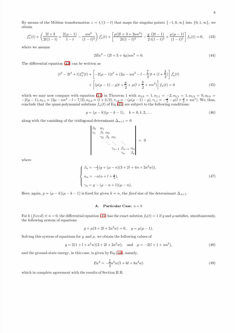
8

By means of the Mobius transformation z = t/(1 − t) that maps the singular points {−1, 0, ∞} into {0, 1, ∞}, weobtain

f ′′n(t) +

2l + 3

2t(1 − t) +

2(µ − 1)

1 − t − wa2

(1 − t)2

f ′n(t) +

µ(2l + 3 + 2wa2)

2t(1 − t)2 − g

2

(2t − 1)

t(1 − t)2 +

µ(µ − 1)

(1 − t)2

f n(t) = 0, (43)

where we assume

2Ea2

−(2l + 3 + 4µ)wa2 = 0. (44)

The differential equation (43) can be written as

(t3 − 2t2 + t)f ′′n (t) +

−2(µ − 1)t2 + (2µ − wa2 − l − 7

2)t + (l +

3

2)

f ′n(t)

+

(µ(µ − 1) − g)t +

g

2 + µ(l +

3

2 + wa2)

f n(t) = 0 (45)

which we may now compare with equation (14) in Theorem 1 with a3,0 = 1, a3,1 = −2, a3,2 = 1, a3,3 = 0, a2,0 =−2(µ − 1), a2,1 = (2µ − wa2 − l − 7/2), a2,2 = (l + 3/2), τ 1,0 = −(µ(µ − 1) − g), τ 1,1 = − g

2 −µ(l + 32 + wa2). We, thus,

conclude that the quasi-polynomial solutions f n(t) of Eq.(45) are subject to the following conditions:

g = (µ

−k)(µ

−k

−1), k = 0, 1, 2, . . . (46)

along with the vanishing of the tridiagonal determinant ∆n+1 = 0

β 0 α1

γ 1 β 1 α2

γ 2 β 2 α3

. . . . . .

. . .γ n−1 β n−1 αn

γ n β n

= 0

where

β n = − 12(g + (µ − n)(3 + 2l + 4n + 2a2w)),

αn = −n(n + l + 12),

γ n = g − (µ − n + 1)(µ − n),

(47)

Here, again, g = (µ − k)(µ − k − 1) is fixed for given k = n, the fixed size of the determinant ∆n+1.

A. Particular Case: n = 0

For k (fixed) ≡ n = 0, the differential equation (45) has the exact solution f 0(t) = 1 if g and µ satisfies, simultaneously,the following system of equations

g + µ(3 + 2l + 2a2w) = 0, g = µ(µ − 1).

Solving this system of equations for g and µ, we obtain the following values of

g = 2(1 + l + a2w)(3 + 2l + 2a2w), and µ = −2(l + 1 + wa2), (48)

and the ground-state energy, in this case, is given by Eq.( 44), namely,

Ea2 = −1

2a2w(5 + 6l + 8a2w) (49)

which in complete agreement with the results of Section II.B.



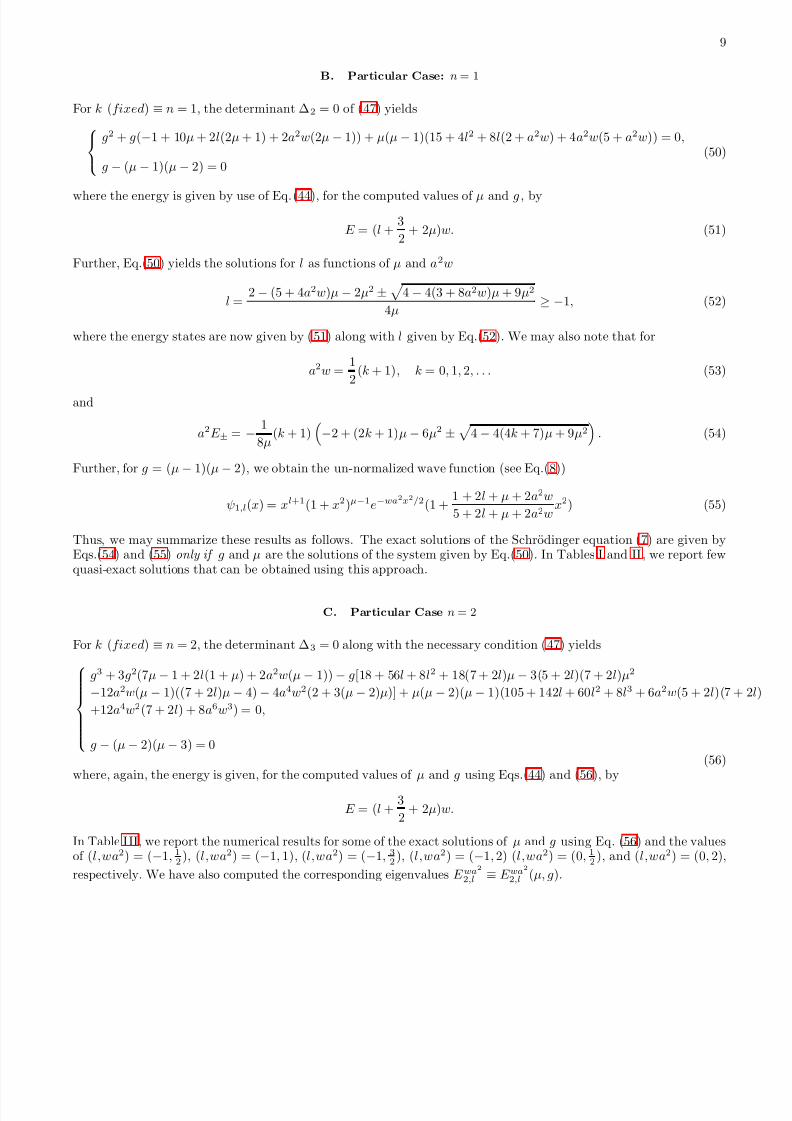
9

B. Particular Case: n = 1

For k (fixed) ≡ n = 1, the determinant ∆2 = 0 of (47) yields

g2 + g(−1 + 10µ + 2l(2µ + 1) + 2a2w(2µ − 1)) + µ(µ − 1)(15 + 4l2 + 8l(2 + a2w) + 4a2w(5 + a2w)) = 0,

g − (µ − 1)(µ − 2) = 0(50)

where the energy is given by use of Eq.(44), for the computed values of µ and g , by

E = (l + 3

2 + 2µ)w. (51)

Further, Eq.(50) yields the solutions for l as functions of µ and a2w

l = 2 − (5 + 4a2w)µ − 2µ2 ±

4 − 4(3 + 8a2w)µ + 9µ2

4µ ≥ −1, (52)

where the energy states are now given by (51) along with l given by Eq.(52). We may also note that for

a2w = 1

2(k + 1), k = 0, 1, 2, . . . (53)

and

a2E ± = − 1

8µ(k + 1)

−2 + (2k + 1)µ − 6µ2 ±

4 − 4(4k + 7)µ + 9µ2

. (54)

Further, for g = (µ − 1)(µ − 2), we obtain the un-normalized wave function (see Eq.(8))

ψ1,l(x) = xl+1(1 + x2)µ−1e−wa2x2/2(1 + 1 + 2l + µ + 2a2w

5 + 2l + µ + 2a2wx2) (55)

Thus, we may summarize these results as follows. The exact solutions of the Schrodinger equation (7) are given byEqs.(54) and (55) only if g and µ are the solutions of the system given by Eq.(50). In Tables I and II, we report fewquasi-exact solutions that can be obtained using this approach.

C. Particular Case n = 2

For k (fixed) ≡ n = 2, the determinant ∆3 = 0 along with the necessary condition (47) yields

g3 + 3g2(7µ − 1 + 2l(1 + µ) + 2a2w(µ − 1)) − g[18 + 56l + 8l2 + 18(7 + 2l)µ − 3(5 + 2l)(7 + 2l)µ2

−12a2w(µ − 1)((7 + 2l)µ − 4) − 4a4w2(2 + 3(µ − 2)µ)] + µ(µ − 2)(µ − 1)(105 + 142l + 60l2 + 8l3 + 6a2w(5 + 2l)(7 +

+12a4w2(7 + 2l) + 8a6w3) = 0,

g − (µ − 2)(µ − 3) = 0(56)

where, again, the energy is given, for the computed values of µ and g using Eqs.(44) and (56), by

E = (l + 3

2 + 2µ)w.

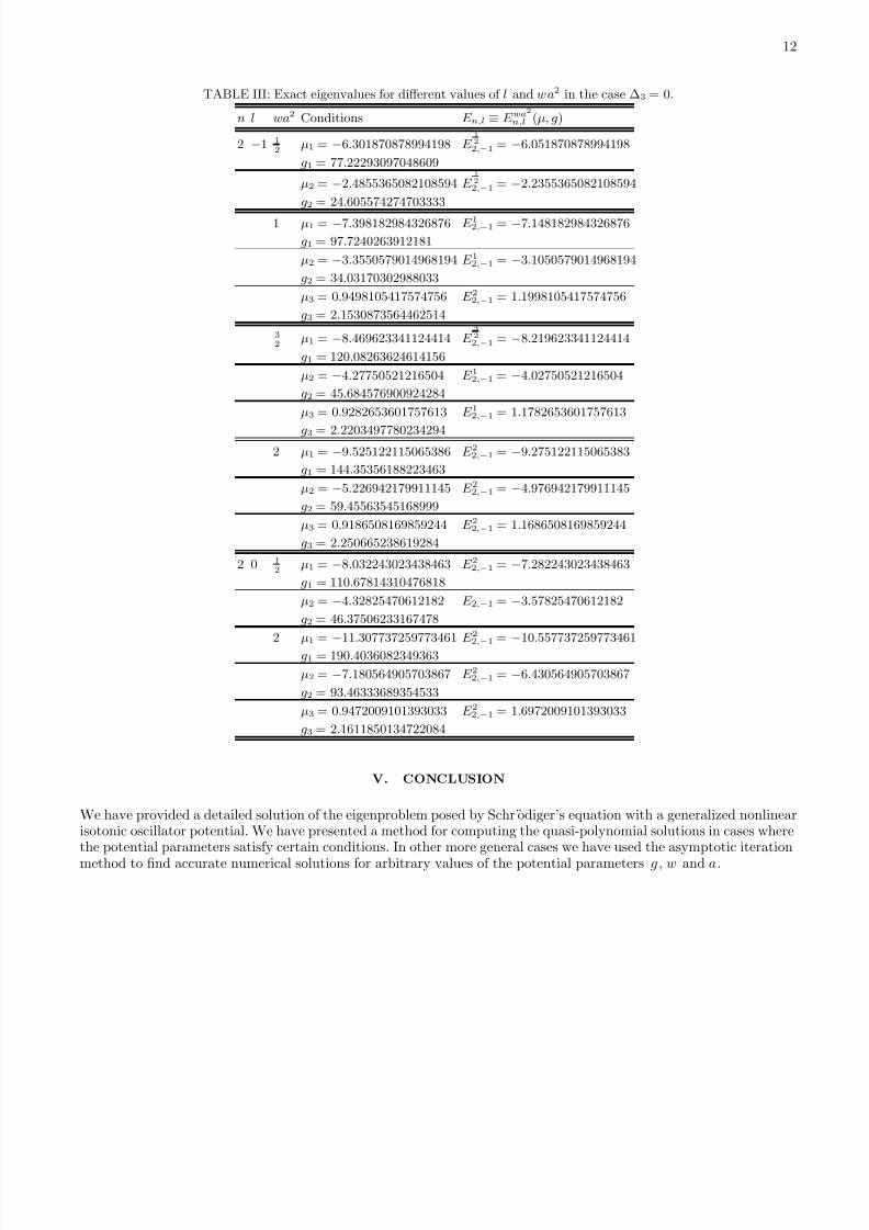
In Table III, we report the numerical results for some of the exact solutions of µ and g using Eq. (56) and the valuesof (l,wa2) = (−1, 1

2), (l,wa2) = (−1, 1), (l,wa2) = (−1, 32), (l,wa2) = (−1, 2) (l,wa2) = (0, 1

2), and (l,wa2) = (0, 2),

respectively. We have also computed the corresponding eigenvalues E wa2

2,l ≡ E wa2

2,l (µ, g).



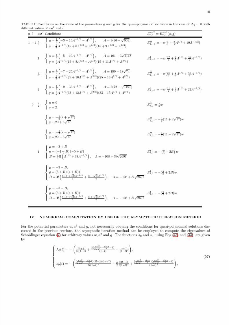
11

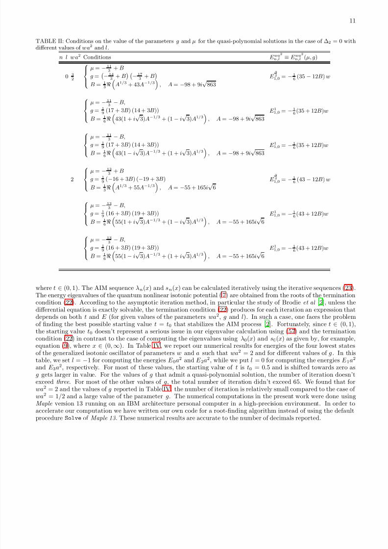
TABLE II: Conditions on the value of the parameters g and µ for the quasi-polynomial solutions in the case of ∆2 = 0 withdifferent values of wa2 and l.

n l w a2 Conditions E wa2

n,l ≡ E wa2

n,l (µ, g)

0 32

µ = − 113

+ B

g =− 14

3 + B −17

3 + B

B = 13ℜ

A1/3 + 43A−1/3

, A = −98 + 9i

√ 863

E 321,0 = − 1

6 (35 − 12B) w

µ = − 113 − B,

g = 19

(17 + 3B) (14 + 3B))

B = 16ℜ

43(1 + i√

3)A−1/3 + (1 − i√

3)A1/3

, A = −98 + 9i√

863

E 11,0 = − 16

(35 + 12B)w

µ = − 113 − B,

g = 19 (17 + 3B) (14 + 3B))

B = 16ℜ

43(1− i√

3)A−1/3 + (1 + i√

3)A1/3

, A = −98 + 9i√

863

E 11,0 = − 16

(35 + 12B)w

2

µ = − 133

+ B

g = 19

(−16 + 3B) (−19 + 3B)

B = 13

ℜA1/3 + 55A−1/3 , A =

−55 + 165i

√ 6

E 32

1,0 = − 16

(43 − 12B) w

µ = − 133 − B,

g = 19

(16 + 3B) (19 + 3B))

B = 16ℜ

55(1 + i√

3)A−1/3 + (1 − i√

3)A1/3

, A = −55 + 165i√

6

E 11,0 = − 16

(43 + 12B)w

µ = − 133 − B,

g = 19

(16 + 3B) (19 + 3B))

B = 16ℜ

55(1− i√

3)A−1/3 + (1 + i√

3)A1/3

, A = −55 + 165i√

6

E 11,0 = − 16

(43 + 12B)w

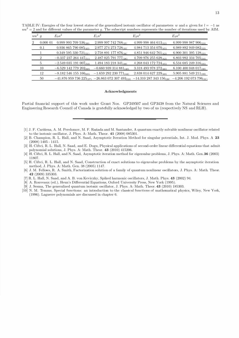
where t ∈ (0, 1). The AIM sequence λn(x) and sn(x) can be calculated iteratively using the iterative sequences (23).The energy eigenvalues of the quantum nonlinear isotonic potential ( 7) are obtained from the roots of the terminationcondition (22). According to the asymptotic iteration method, in particular the study of Brodie et al [2], unless thedifferential equation is exactly solvable, the termination condition (22) produces for each iteration an expression thatdepends on both t and E (for given values of the parameters wa2, g and l). In such a case, one faces the problemof finding the best possible starting value t = t0 that stabilizes the AIM process [2]. Fortunately, since t ∈ (0, 1),the starting value t0 doesn’t represent a serious issue in our eigenvalue calculation using (57) and the terminationcondition (22) in contrast to the case of computing the eigenvalues using λ0(x) and s0(x) as given by, for example,equation (9), where x ∈ (0, ∞). In Table IV, we report our numerical results for energies of the four lowest statesof the generalized isotonic oscillator of parameters w and a such that wa2 = 2 and for different values of g . In thistable, we set l = −1 for computing the energies E 0a2 and E 2a2, while we put l = 0 for computing the energies E 1a2

and E 3a2, respectively. For most of these values, the starting value of t is t0 = 0.5 and is shifted towards zero asg gets larger in value. For the values of g that admit a quasi-polynomial solution, the number of iteration doesn’t

exceed three . For most of the other values of g, the total number of iteration didn’t exceed 65. We found that forwa2 = 2 and the values of g reported in Table IV, the number of iteration is relatively small compared to the case of wa2 = 1/2 and a large value of the parameter g. The numerical computations in the present work were done usingMaple version 13 running on an IBM architecture personal computer in a high-precision environment. In order toaccelerate our computation we have written our own code for a root-finding algorithm instead of using the defaultprocedure Solve of Maple 13 . These numerical results are accurate to the number of decimals reported.



12

TABLE III: Exact eigenvalues for different values of l and wa2 in the case ∆3 = 0.

n l wa2 Conditions E n,l ≡ E wa2

n,l (µ, g)

2 −1 12

µ1 = −6.301870878994198 E 12

2,−1 = −6.051870878994198

g1 = 77.22293097048609

µ2 = −2.4855365082108594 E 12

2,−1 = −2.2355365082108594

g2 = 24.605574274703333

1 µ1 = −7.398182984326876 E 12,−1 = −7.148182984326876

g1 = 97.7240263912181

µ2 = −3.3550579014968194 E 12,−1 = −3.1050579014968194

g2 = 34.03170302988033

µ3 = 0.9498105417574756 E 22,−1 = 1.1998105417574756

g3 = 2.1530873564462514

32

µ1 = −8.469623341124414 E 32

2,−1 = −8.219623341124414

g1 = 120.08263624614156

µ2 = −4.27750521216504 E 12,−1 = −4.02750521216504

g2 = 45.684576900924284

µ3 = 0.9282653601757613 E 12,−1 = 1.1782653601757613

g3 = 2.22034977802342942 µ1 = −9.525122115065386 E 22,−1 = −9.275122115065383

g1 = 144.35356188223463

µ2 = −5.226942179911145 E 22,−1 = −4.976942179911145

g2 = 59.45563545168999

µ3 = 0.9186508169859244 E 22,−1 = 1.1686508169859244

g3 = 2.250665238619284

2 0 12

µ1 = −8.032243023438463 E 22,−1 = −7.282243023438463

g1 = 110.67814310476818

µ2 = −4.32825470612182 E 2,−1 = −3.57825470612182

g2 = 46.37506233167478

2 µ1 =−

11.307737259773461 E 22,−1 =

−10.557737259773461

g1 = 190.4036082349363

µ2 = −7.180564905703867 E 22,−1 = −6.430564905703867

g2 = 93.46333689354533

µ3 = 0.9472009101393033 E 22,−1 = 1.6972009101393033

g3 = 2.1611850134722084

V. CONCLUSION

We have provided a detailed solution of the eigenproblem posed by Schr odiger’s equation with a generalized nonlinearisotonic oscillator potential. We have presented a method for computing the quasi-polynomial solutions in cases wherethe potential parameters satisfy certain conditions. In other more general cases we have used the asymptotic iteration

method to find accurate numerical solutions for arbitrary values of the potential parameters g , w and a.



13

TABLE IV: Energies of the four lowest states of the generalized isotonic oscillator of parameters w and a given for l = −1 aswa2 = 2 and for different values of the parameter g . The subscript numbers represents the number of iterations used by AIM.

wa2 g E 0a2 E 1a2 E 2a2 E 3a2

2 0.000 01 0.999 993 709 536(39) 2.999 997 742 768(25) 4.999 998 464 613(32) 6.999 998 987 906(23)

0.1 0.936 865 790 085(43) 2.977 274 273 728(33) 4.984 713 354 070(45) 6.989 892 949 082(32)

1 0.349 595 330 721(51) 2.758 891 177 876(36) 4.851 946 642 761(42) 6.900 301 395 128(35)

2 −0.337 237 264 447(51) 2.487 025 791 777(38) 4.709 976 255 628(42) 6.803 992 334 705(34)5 −2.549 035 191 007(53) 1.494 183 218 341(39) 4.268 043 172 724(45) 6.534 685 249 316(35)

10 −6.529 142 779 202(60) −0.660 939 314 881(40) 3.318 493 978 272(46) 6.100 400 048 017(38)

12 −8.182 546 155 166(65) −1.659 292 230 771(44) 2.838 014 627 229(48) 5.905 881 549 211(39)

50 −41.876 959 736 225(37) −26.863 072 307 493(33) −14.310 287 343 156(28) −4.206 192 073 796(31)

Acknowledgments

Partial financial support of this work under Grant Nos. GP249507 and GP3438 from the Natural Sciences andEngineering Research Council of Canada is gratefully acknowledged by two of us (respectively NS and RLH).

[1] J. F. Carinena, A. M. Perelomov, M. F. Ranada and M. Santander, A quantum exactly solvable nonlinear oscillator relatedto the isotonic oscillator, J. Phys. A: Math. Theor. 41 (2008) 085301.

[2] B. Champion, R. L. Hall, and N. Saad, Asymptotic Iteration Method for singular potentials, Int. J. Mod. Phys. A 23

(2008) 1405 - 1415.[3] H. Ciftci, R. L. Hall, N. Saad, and E. Dogu, Physical applications of second-order linear differential equations that admit

polynomial solutions, J. Phys. A: Math. Theor. 43 (2010) 415206.[4] H. Ciftci, R. L. Hall, and N. Saad, Asymptotic iteration method for eigenvalue problems, J. Phys. A: Math. Gen. 36 (2003)

11807.[5] H. Ciftci, R. L. Hall, and N. Saad, Construction of exact solutions to eigenvalue problems by the asymptotic iteration

method, J. Phys. A: Math. Gen. 38 (2005) 1147.[6] J. M. Fellows, R. A. Smith, Factorization solution of a family of quantum nonlinear oscillators, J. Phys. A: Math. Theor.

42 (2009) 335303.

[7] R. L. Hall, N. Saad, and A. B. von Keviczky, Spiked harmonic oscillators, J. Math. Phys. 43 (2002) 94.[8] A. Ronveaux (ed.), Heun’s Differential Equations, Oxford University Press, New York (1995).[9] J. Sesma, The generalized quantum isotonic oscillator, J. Phys. A: Math. Theor. 43 (2010) 185303.

[10] N. M. Temme, Special functions: an introduction to the classical functions of mathematical physics, Wiley, New York,(1996). Laguerre polynomials are discussed in chapter 6.

oscillator quantic mecanic

Documents

Transcript of oscillator quantic mecanic