ORCA labs 6 Frontier orbitals - University of...

PART II – ADVANCED AND SPECIAL SUBJECTS 1

PART II

ADVANCED AND SPECIAL SUBJECTS


1 Computer Experiment 7: Interpretation of Structure, Bonding and Reactivity Using Orbitals

1.1 Background

1.1.1 Hückel MO Theory The Hückel theory is the simplest semi-‐empirical method for the description of

molecular systems. It was developed in 1931 by Erich Hückel for the calculation of

planar conjugated hydrocarbons. Later Hoffmann generalized this very successful

concept to general molecules and applied it with great success to many areas of

chemistry. He termed his method the “extended Hückel theory” (EHT). The appeal of

the Hückel and EHT methods is that they can provide many qualitative insights into

the behaviour of molecules, in particular of molecules that are closely related.1 It

does not, however, provide reliable numbers. For this purpose ab initio or DFT

methods must be consulted.2

A. Extended Hückel MO theory

EHT theory might be thought of as an essentially very simple, semiempirical

approximation of Hartree-‐Fock theory. In Hartree-‐Fock theory, a single Slater

determinant is taken as an Ansatz for the description of the N-‐electron system. The

single determinant is composed of one-‐particle molecular orbitals (MOs) that are

found as solutions to a pseudo-‐eigenvalue problem of the form:

F!i= "

i!

i

( 1)

Where F is the „Fock operator“, which describes the motion of a single electron in

the field of the nuclei and the remaining electrons.The MOs are written as a linear

combination of atomic orbitals (LCAO-‐Ansatz):

1 Recommended literature to this chapter is: Ian Fleming, Grenzorbitale und Reaktionen organischer Verbindungen, VCH 1990 2 Even today it might not be a bad idea to do a few simple EHT calculations at the beginning of a project if one has no familiarity with the systems being investigated and to use the results to gain some feeling for the factors that might be worthwhile to examine with more rigorous electronic structure methods.


!

ir( ) = c

µi"

µr( )

µ!

( 2) After which the calculation boils down to the solution of a generalized eigenvalue

problem for the determination of the unknown MO coefficients c

µi and the orbital

energies !i

Fc = !Sc

( 3)

Where ! is a diagonal matrix with orbital energies and the matrix elements of the

Fock matrix F and the overlap matrix S are defined by:

F

µ!= "

µF "

!

( 4)

S

µ!= "

µ"!

( 5) As pointed out in the introduction, Hartree-‐Fock calculations require the use of large

basis sets and iterative cycles for the optimization of the MOs. In EHT theory, one

focuses on the qualitative shape of the valence orbitals and usually pays attention to

those orbitals that are located near the HOMO-‐LUMO gap (the “frontier orbitals”).

According to frontier molecular orbital theory (described below in chapter 1.1.3)

these are the most important ones for the reactivity of the system. In order to get an

impression of how these orbitals may look like it is not necessary to solve the rather

laborious HF equations – in fact this was a major challenge for all but the smallest

molecules in the 1960s when EHT theory was suggested – it is enough to replace the

Fock operator by a semiempirical effective one-‐electron operator heff and to only

consider the “minimal” chemical set of valence orbitals3 as !{ } . It is not necessary

to specify the operator heff precisely. In order to solve eq (3), it is only necessary to

specify the matrix elements of this operator. In EHT theory they are given by:

3 For example, for a carbon atom one includes 2s, 2px, 2py and 2pz and for titanium one would use 3dxy, 3dx2-‐y2, 3dxz, 3dyz, 2dz2-‐r2, 4s and perhaps also 4px, 4poy and 4pz.


hµ!eff = "

µheff "

!=

#µ

if µ = !

$µ!

if µ ! !

"#$$$

%$$$

( 6)

The diagonal elements ! µ represent the “energy of the atomic orbital !µ in the free

atom”. It is approximated by the so-‐called “valence shell ionization energy” (VOIP)

which can be determined from atomic spectroscopy.4 These numbers are negative

and represent the average energy required to remove an electron from the given

orbital (2s, 2p, 3d, …) The lower these energies, the higher the electron attracting

ability of the atom. The off-‐diagonal matrix elements are called “resonance

integrals”. They measure the strength of the interaction between two atomic

orbitals. Intuitively, it is reasonable to expect that these integrals are related to the

overlap integrals. Thus, in EHT they are given by:5

!µ" =

12 KSµ" # µ +#"( )

( 7)

The constant K ~ 1.75 is an empirical constant to adjust the resonance integrals to

more reasonable values given that the form of eq (7) is an oversimplification. In

order to provide a feel for the values of the parameters we give them for elements

H-‐Ne in Table 1:. Table 1: VOIPs for elements H-‐Ne to be used together with EHT calculations. Note, that the negative of the values listed below is to be used.

Element αs (eV) αp (eV) H 13.61 -‐ He 24.59 -‐ Li 5.39 3.60 Be 9.32 6.00 B 12.93 8.30 C 16.59 11.26 N 20.33 14.53

4 The values of these parameters are tabulated in multiple places. Since there are many ways to determine these parameters from the experimental data, no consensus has been reached in the community about a “universal” set of VOIPs. 5 There are many modifications of the formulas for the off-‐diagonal. It is questionable if any of these is really to be preferred over another one and in this situation “Ockham’s razor” principle applies which essentially states that the simplest solution is just as good as any.


O 28.48 13.62 F 37.85 17.42 Ne 48.47 21.61

Following the solution of the generalized eigenvalue problem in eq (3) and with the

approximation described above, the resulting MOs are filled in order of increasing

energy with the available electrons in keeping with the “Aufbau principle” in order

to find the electronic ground state. Since the approximations are so simple, the total

energy in the EHT method is simply the sum of orbital energies:

E EHT = ni! i

i" ( 8)

Where ni is the occupation number of the i’th orbital (=0,1 or 2). In connection with

Walsh’s rules, we will see below that the variations of the orbital energies with

geometry can be used to obtain quite important and general insights about the

geometric structures of molecules. In fact, many areas of chemistry have profited

from performing such qualitative calculations.

B. Hückel theory for π electron systems (HMO)

Although it existed prior to EHT theory, the HMO theory of aromatic π-‐systems

might be thought of as a further simplification of the EHT method. In this case, one

only considers the π-‐electrons of the investigated molecules and only keeps the pz

orbitals of the atoms involved in the π-‐system. Substituent effects are included in an

approximate manner by modifying the α-‐parameters of the atoms to which the

substituents are attached. Furthermore, in HMO theory, the off-‐diagonal elements of

the overlap matrix are neglected such that the final eigenvalue problem to be solved

is:

heff c = !c

( 9)

Finally, one only keeps resonance integrals between atoms that are nearest

neighbours and assigns a constant value to them. Thus, the calculations also become

geometry independent and the only thing that is required in order to perform a

HMO calculation is a molecular connectivity. Although these approximations clearly


represent a gross oversimplification of the molecular electronic structure problem,

it can hardly be overemphasized how much HMO theory has shaped chemical

thinking about aromatic molecules and their properties.6 However, we will not

pursue HMO theory in this course but stay in the framework of the EHT method

below.

1.1.2 Walsh’s Rules7 Walsh diagrams are the graphical representation of the MO energies in dependence

of a geometrical parameter, most commonly a bond angle. For example, consider the

case of the H3 molecule in its linear and triangular forms as shown in Figure 1. It is

observed that upon bending, the energy of the nonbonding σu orbital (it correlates

with a b2 orbital in C2v symmetry) strongly increases and finally correlates with one

component of the antibonding e-‐orbital in the final D3h structure. Since there are

three electrons to be filled into the three MOs, it is predicted that H3 should be linear

((1σg)2(1σu)1 configuration) while H3+ should be triangular ((a1)2 configuration)

since the a1 orbital is stabilized upon bending.

Figure 1: Walsh diagram for the distortion of the H3 system.

The variation of a geometrical degree of freedom may cause a crossing of different

MO-‐levels. In general, such a crossing is allowed if the two MOs transform under

different irreducible representations and is avoided otherwise.(the famous non-‐

crossing rule; compare Figure 2). The non-‐crossing rule is particularly important for

the interpretation of photochemical reactions. The occurrence of a HOMO / LUMO

6 The classic text on HMO theory is E. Heilbronner, H. Bock “Das HMO Modell und seine Anwendung”. Verlag Chemie, Weinheim/Bergstrasse, 1968 7 For a detailed ab initio perspective on Walsh’s rules see: Buenker, R.J.M; Peyerimhoff, S.D. Chem. Rev., 1974, 74, 127

The image cannot be displayed. Your computer may not have enough memory to open the image, or the image may have been corrupted. Restart your computer, and then open the file again. If the red x still appears, you may have to delete the image and then insert it again.


crossing with identical symmetry implies that the reaction is symmetry forbidden,

due to the non-‐conservation of the orbital symmetry of the occupied MOs. Therefore

a high activation energy is expected.

Figure 2: Crossing and avoided crossing of two energy levels.

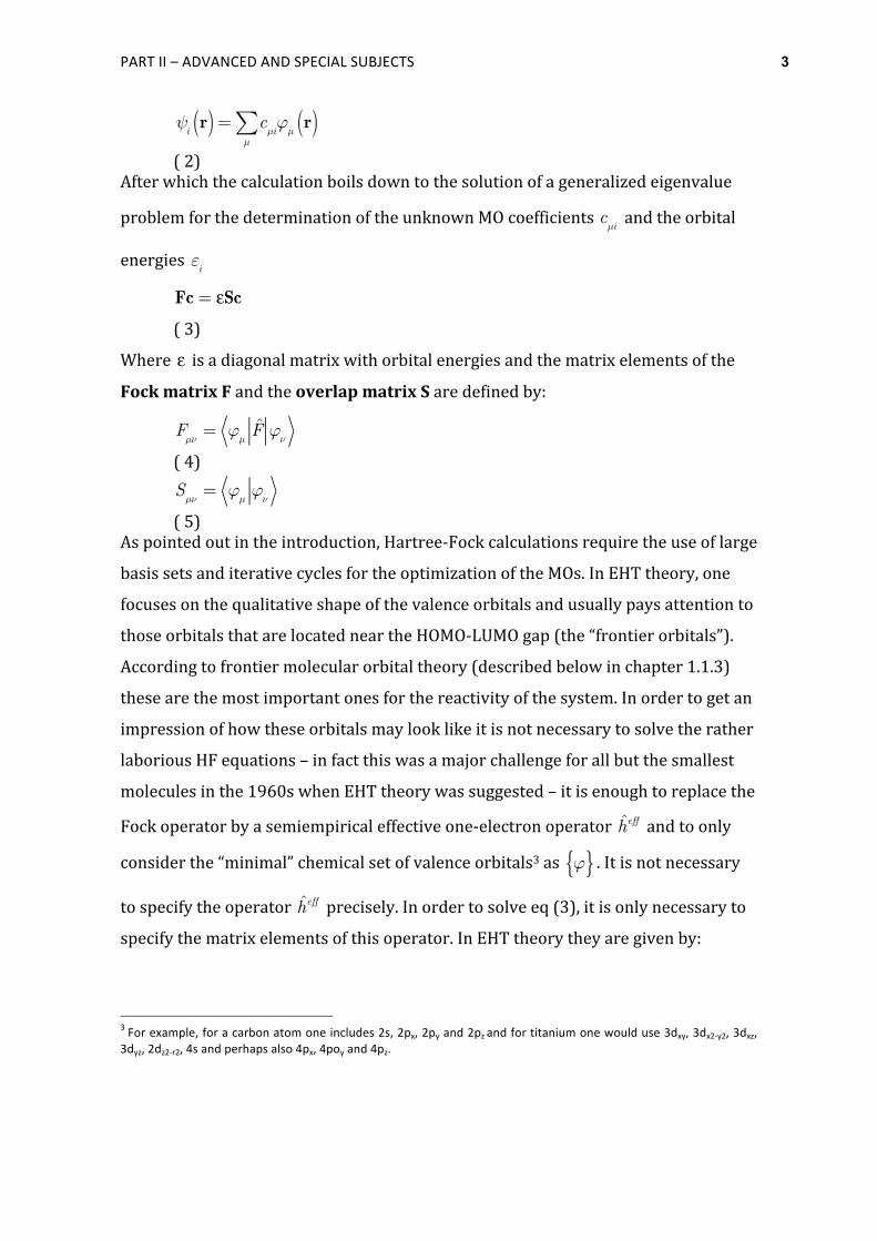
In Figure 3 the Walsh diagram for the bending mode of a AH2 molecule is shown.

The energy of the lowest valence MOs decrease upon bending as three center

bonding between s-‐AOs becomes more favourable in the bent form. The 1 σu-‐MO is

strongly bonding in the linear case, but upon reducing the angle, the 1b2-‐MO

becomes only weakly bonding, because in the linear case the 2py-‐AOs can interact

more strongly with the AOs of the H-‐atoms. The 1 πu-‐MO separates in two

components, 1b1 and 3a1. The energy of the 1b1 MO is almost constant while the 3a1-‐

MO becomes a bonding MO upon bending. The overlap of the 2pz-‐AOs from A with

1s-‐AOs from the H-‐atoms is zero in the linear case, but reducing the angle results in

a three-‐center bonding.



Figure 3: Walsh diagram for a AH2 molecule.8

1.1.3 Approximate Intermolecular Interactions In this section we will indicate how the energies and shapes of molecular orbitals

can be related to chemical reactivity. One of the key features of chemical reactions is

the activation energy that has to be overcome by the reactants. On the basis of

perturbation theory and EHT, Klopman and Salem [G. Klopman, JACS, 90, 223

(1968); S. Salem, JACS, 90, 543 (1968)] developed a simple but highly useful

decomposition scheme for the interaction energy ΔE of two approaching molecules

A and B into contributions from occupied and unoccupied orbitals. All quantities in

(10) are obtained for the separate, non-‐interacting molecules.

!E =" (qµ

+q!)"

µ!µ!

A,B

# Sµ!

+Q

IQ

J

#RIJI<J

#

+2( c

aµc

q!"

µ!)2

µ!#

Ea"E

qq

unocc

#a

occ

# +2( c

bµc

p!"

µ!)2

µ!#

Eb"E

pp

unocc

#b

occ

#

( 10) This expression – although somewhat lengthy – is already simplified (the approach

does not take electron-‐electron interaction into account). So let us discuss the terms

step by step. The first term is a double sum over all atomic orbitals (AOs) μ of

8Kutzelnigg, W., Einführung in die Theoretische Chemie Band 2, VCH: Weinheim, 1994




molecule A and ν of molecule B. The q’s are the AO occupation numbers of the non-‐

interacting molecules (in the original paper called charge densities), β is similar but

not identical to the resonance integral of Hückel theory (it includes only the

electron-‐nuclear attraction terms), and S is the overlap integral mentioned

previously. Since β is always negative, this term is positive and is basically

responsible for the occurrence of activation barriers within this model. Its origin is

the repulsive interaction between doubly occupied molecular orbitals (MOs) of A

and B which arises from the non-‐symmetric level splitting (Figure 4).

Figure 4: Interaction of Two Occupied Molecular Orbitals

The second term, a sum over all atoms I of molecule A and atoms J of molecule B,

describes the Coulomb interaction between pairs of atoms with net charge Q at

distance R (ε is the dielectric constant). The two last terms include sums over all

occupied MOs a of A and unoccupied MOs q of B and vice versa. For each pair of

orbitals the term consists of sums of corresponding MO coefficients c weighted with

β. The dominator is the MO energy difference. This part describes the stabilization

due to formation of orbitals combining occupied A MOs with unoccupied B MOs or

vice versa in the complex [AB]*.

Figure 5: Interaction of an Occupied and an Unoccupied Orbital.


1.1.4 Frontier orbital picture It is exactly this last effect which is widely used in further simplified qualitative

approaches to determine chemical reactivity. If the two reacting molecules are

similar, the smallest energy differences are those between the highest occupied MOs

(HOMOs) and the lowest unoccupied MOs (LUMOs). If it is assumed that the other

contributions to the last two terms of (1) are always of similar magnitude, the

HOMO-‐LUMO contributions will dominate. If it is further assumed that the first term

is roughly independent from the intermolecular orientation, only two main

contributions are left for the determination of the feasibility and, sometimes even

more important, the regioselectivity of chemical reactions: the Coulomb term and

the MO coefficients of the frontier orbitals, HOMO and LUMO.

This concept is used e.g. to estimate the relative reactivity of different compounds C

towards a given reactant R via calculation of E(HOMO,C)-‐E(LUMO,R)+E(HOMO,R)-‐

E(LUMO,C).

The frontier orbital approach is also applied to ionic reactions in organic chemistry.

In electrophilic or nucleophilic reactions the inorganic ions are classified as hard or

soft. A hard nucleophilic has a low HOMO energy, a hard electrophilic has a high

LUMO energy, and vice versa. In nucleophilic reactions, a hard anion (e.g. OH-‐, NH2-‐)

will attack preferentially the atom with the highest positive charge Q of an organic

molecule. In the frontier orbital picture this is due to the large energetic difference

between the anion’s HOMO and the molecule’s LUMO making the last term in the

above equation small so that the Coulomb part prevails. On the other hand, the

preferred site for a soft anion (CN-‐, (CH2,Ph)-‐C-‐O-‐) is the atom with the largest

contribution to the molecule’s LUMO.

1.1.5 The Woodward-‐Hoffman Rules In reaction theory synchronous organic reactions such as pericyclic reactions would

in general take place under preservation of the orbital symmetry. Each occupied MO

of the reactants will result in an occupied MO of the products with the same

symmetry. Experimentally, there are two ways of activating such reactions:

1. Thermal activation


2. Photochemical activation

For the theoretical description, the main difference between these two methods lies

in the MOs that are involved in these processes. The photochemical activation will

result in the excitation of an electron from a bonding (or nonbonding) into an anti-‐

bonding orbital. The resulting state may have a different symmetry than the ground

state and will therefore also have a distinct reactivity (Figure 6). Essential difference

between photochemical and thermal reactions must therefore be expected and are

also observed in practice.

Figure 6: The orbitals that are involved in the different activation cases.9

A. Electro-‐cyclic reactions

Electro-‐cyclic reactions may be described as an isomerisation of open-‐chain polyens

to ring isomers which takes place under thermal or photochemical activation. In

order to close the ring an additional σ-‐bond has to created at the expense of a π-‐

bond. In EHT language, the π-‐MOs on one fragment have to overlap with correct

phases with the orbitals of another fragment in order to form a σ-‐bond. The

example of 1,3-‐Butadiene is shown above in (Figure 6). In fact, it can be determined

in advance, when a suitable constructive overlap of the π-‐orbitals is possible – it 9Woodward, R. B.; Hoffmann R. Angew. Chem. 81. Jahrgang 1969, 21, 797



simply depends on the number of π-‐electrons. As long as both fragments stay in

their electronic ground state 4n (n=1,2,...) π-‐electrons in the molecule lead ti in-‐

phase arrangement of the terminal π-‐orbitals, whereas 4n+2 (n=1,2,...) π-‐electrons

result in an out-‐of-‐phase arrangement. In order to build up a new σ-‐bond, the π-‐

orbitals in the molecule with 4n π-‐electrons have to rotate in the same direction

(conrotatory) in order to result in a bonding orbital, while the molecules containing

4n+2 π-‐electrons are obliged to rotate in opposite directions (disrotatory) (compare

Figure 7) For photochemical reactions the requirements for constructive overlap

are exactly the reverse of the one described above. Therefore, a system with 4n π-‐

electrons has to rotate in opposite directions, whereas a system containing 4n+2 π-‐

electrons needs to rotate in the same direction. Since the two possibilities lead to

different stereoisomers of the products that are formed (Figure 7), one can readily

predict whether one has to activate a given reaction photochemically or thermally in

order to obtain the desired product.

Figure 7: Example for con-‐ and dis-‐rotatory rotation of the terminal pz orbitals in case of thermal activation



Table 2: Summary of allowed and forbidden electrocyclic reactions based on the Woodward-‐Hoffman rules.

m+n-electro-cyclic reactions Thermal activation

ground state

Photochemical activation

excited state

forbidden allowed allowed forbidden

M+n = 4q q=1, 2,... disrotatory conrotatory disrotatory conrotatory M+n = 4q + 2 q=1, 2,... conrotatory disrotatory conrotatory disrotatory

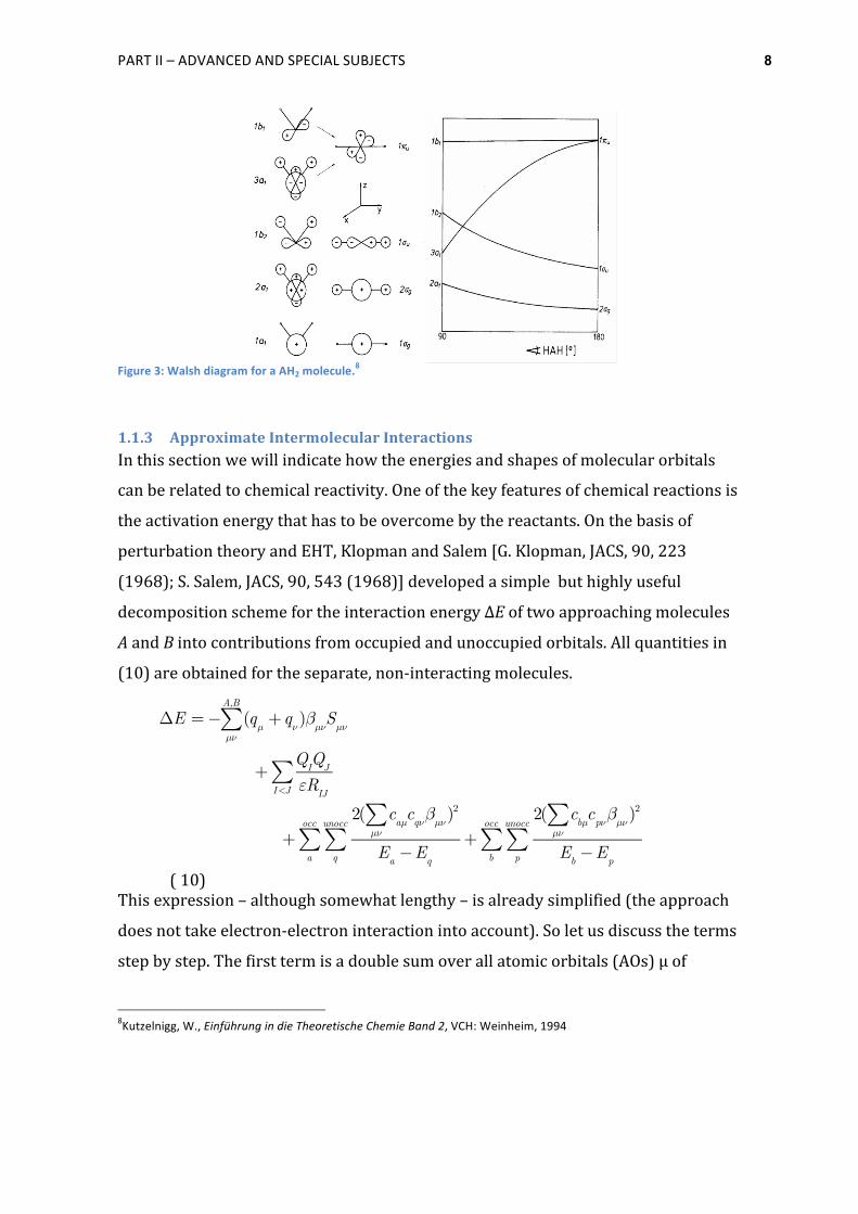
B. Cycloadditions

In concerted cycloadditions two new σ-‐bonds are built up due to overlap of the π-‐

orbitals of both reactants. The location of the σ-‐bond is arranged either on the same

side of the reacting π-‐system or on the opposite side. The first case is referred to as

a “suprafacial” reaction and the second case as a “antarafacial” process. The

alignment of the “responsive” π-‐orbitals is again dependent on the number of π-‐

electrons and on the form of activation as summarized in Figure 8, Figure 9 and

Table 3.

Figure 8: Orbital symmetry of a photochemical cyclic addition.




Figure 9: Orbital symmetry of a thermal cyclic addition. (a) anti-‐binding (b) binding, but geometrically difficult



Table 3: Summary of the Woodward-‐Hoffman rules.

m+n-cyclic addition Thermal activation

ground state

Photochemical activation

excited state

forbidden allowed allowed forbidden

m+n = 4q q=1, 2,... Πma + Πna antara, antara

Πms + Πna supra, antara

Πms + Πns supra, supra

Πma + Πns antara, supra

m+n = 4q + 2 q=1, 2,... Πma + Πns antara, supra

Πms + Πns supra, supra

Πms + Πna supra, antara

Πma + Πna antara, antara

1.1.6 Limitations of the Frontier Molecular Orbital Approach Although the above scheme has been proven to give qualitatively correct

predictions in many cases, as we will see below, it is of course limited due to its

approximate nature. From the quantum-‐chemical viewpoint, it is mainly the use of

atomic charges and LUMO energy and shape that makes the simple approach

questionable. Atomic charges are no observables and strongly depend on the

analysis and the basis set. But also the shape of the orbitals is method and basis set

dependent. The MOs employed in the above analysis are obtained with minimal

basis sets in the extended Hückel framework. Nowadays, one of course wants to go

beyond this simple level of theory and use HF or DFT calculations as basis for

analysis of chemical reactivity. And here arises a fundamental problem: For a given

method, the HOMO converges to something definite while the unoccupied orbitals

do not. Remember that only the occupied orbitals, either included in the Slater

determinant in HF theory or used to calculate the electron density in DFT, are

optimized by the variation procedure. The only criterion for unoccupied orbitals is

their orthogonality to the occupied space. In the limit of a complete basis set, the

unoccupied space forms a continuum and the LUMO is not really defined. We will

demonstrate this in an example in this experiment. In HF theory even the energies

Ep, Eq of the unoccupied MOs are fundamentally wrong because the fictitious

(virtual) electrons in the UMOs experience the repulsive field of all N electrons of


the system, whereas the occupied orbitals experience the correct N-‐1 electron

potential. Their energy can be related to physical properties (ionization energies)

via the Koopmans theorem. The situation in DFT is not much better. Here the virtual

MOs experience the correct N-‐1 electron repulsive field, but the energies Ea, Eb of the

occupied MOs are incorrect due to artificial self-‐interaction of the electrons which is

caused by the approximate description of electron exchange in DFT. As a

workaround of the above mentioned shortcomings of HF and DFT, hybrid methods

such as B3LYP have been developed where the electron exchange is described by a

mixture of the exact one-‐determinant expression provided by HF theory and a

density functional. The mixing coefficient is usually treated as an empirical

parameter. Its value is determined by optimal reproduction of experimental

properties (including ionization energies and optical spectra). In this way one uses

the cancellation of the inherent errors of both approaches.

Having this in mind, it is not surprising that the frontier orbital approach fails in

some cases. Nevertheless, as a qualitative tool to understand fundamental reasons

for the course of chemical reactions, it is still worth to discuss.

1.2 Description of the Experiment

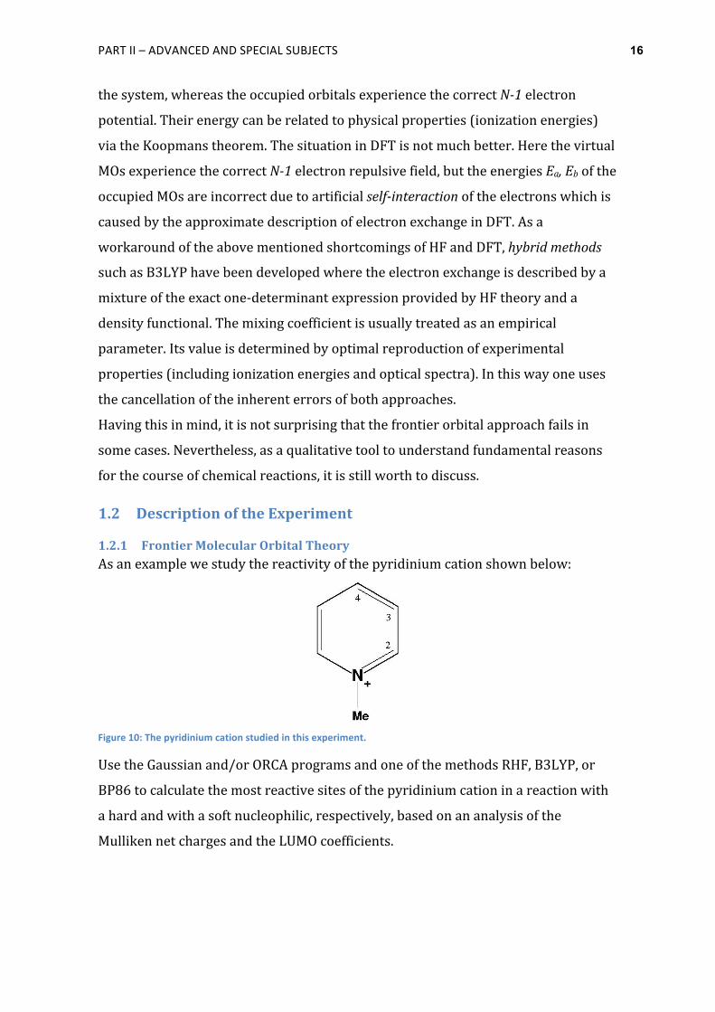
1.2.1 Frontier Molecular Orbital Theory As an example we study the reactivity of the pyridinium cation shown below:

Figure 10: The pyridinium cation studied in this experiment.

Use the Gaussian and/or ORCA programs and one of the methods RHF, B3LYP, or

BP86 to calculate the most reactive sites of the pyridinium cation in a reaction with

a hard and with a soft nucleophilic, respectively, based on an analysis of the

Mulliken net charges and the LUMO coefficients.


Create the molecular structure as described in previous experiments, perform a

structure optimization and analyse the wavefunction of the final structure.

Check if the Mulliken net charges and the shape of the LUMO change if you increase

the basis set from SVP to TZVP. Will the qualitative results of the frontier orbital

analysis change? Hint: instead of analysing the MO coefficients it is sufficient to

draw an orbital picture using MOLDEN or MOLEKEL. In any case the keyword

POP=FULL is needed in Gaussian (ORCA prints a Loewdin analysis of each MO by

default).

Experimentally it is known that hard nucleophilics (OH-‐, NH2-‐) prefer C(2), and soft

nucleophilics (CN-‐, (CH2,Ph)-‐C-‐O-‐) prefer C(4).

Verify the relative reactivity of the two sites versus OH-‐ and CN-‐ by calculating the

energy difference of the four transition structures CN(2), CN(4), OH(2) and OH(4) as

shown below. In this case it is sufficient to fully optimize the structures, no TS

search is necessary.

Figure 11: Structures of the Reaction Products to be Optimized

1.2.2 The Woodward-‐Hoffman Rules

- Dissociation of formaldehyde

Use the ORCA program to optimize the following structures employing HF/6-‐311G*


and generate .cube files for each MO using orca_plot. Alternatively, you can use the

Gaussian program employing HF/6-‐311G* and generate .chk files.

A. H2C=O

B. CO

C. H2 Classify the HF valence orbitals and the lowest unoccupied orbitals according to

their irreducible representation (irrep). Investigate the orbital symmetry

concerning the symmetry elements of the point group C2v.

• Identity (E)

• two-‐fold rotation axis (C2)

• mirror-‐plane in the xz-‐plane (σxz)

• mirror-‐plane in the yz-‐plane (σyz)

Figure 12: Coordinate system used in this experiment.

Table 4: The character table of the C2v point group.

C2v E C2 σxz σyz

A1 1 1 1 1 z x2, y2, z2

A2 1 1 -1 -1 Rz xy

B1 1 -1 1 -1 x, Ry xz



B2 1 -1 -1 1 y, Rx

• Draw a MO diagram for H2C=O on the one side and for CO + H2 on the other side. Connect orbitals which belong to the same irrep with each other.

• Repeat these steps in Cs symmetry with the symmetry elements E and σ. Remember that there are two possibilities for the orientation of formaldehyde in this point group. What should attract your attention?

1.2.3 Walsh’s Rules Perform calculations on the following molecules with the Hartree-‐Fock method and the SVP basis set and the ORCA program:

• LiH2+ (distance= 1.7 Angström)

• BeH2 (distance= 1.34 Angström)

• CH2 (S=0; RKS calculation) (distance=1.078 Angström)

• CH2 (S=1; ROHF calculation; keyword ! ROHF) (distance 1.078 Angström)

• H2O (distance=0.956 Angström)

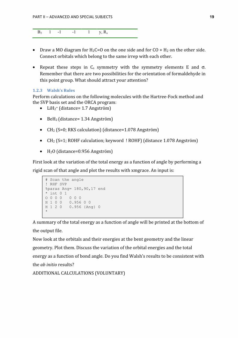
First look at the variation of the total energy as a function of angle by performing a

rigid scan of that angle and plot the results with xmgrace. An input is:

A summary of the total energy as a function of angle will be printed at the bottom of

the output file.

Now look at the orbitals and their energies at the bent geometry and the linear

geometry. Plot them. Discuss the variation of the orbital energies and the total

energy as a function of bond angle. Do you find Walsh’s results to be consistent with

the ab initio results?

ADDITIONAL CALCULATIONS (VOLUNTARY)

# Scan the angle ! RHF SVP %paras Ang= 180,90,17 end * int 0 1 O 0 0 0 0 0 0 H 1 0 0 0.956 0 0 H 1 2 0 0.956 {Ang} 0 *


Plot the variation of the nuclear repulsion energy, the one-‐electron energy, the two-‐

electron energy as well as the kinetic energy of the system as a function of angle.

Also plot the sum of the occupied MO energies weighted by their occupancy as a

function of bond angle. These data must be extracted from the ORCA output file.

What do you find? What is the physical reason for obtaining a bent geometry versus

a linear geometry?.

ORCA labs 6 Frontier orbitals - University of...

Documents

Transcript of ORCA labs 6 Frontier orbitals - University of...