IT 11 010

Examensarbete 30 hpApril 2011

Orbit Segmentation for Cranio- Maxillofacial Surgery Planning

Johan Nysjö

Institutionen för informationsteknologiDepartment of Information Technology

2

Teknisk- naturvetenskaplig fakultet UTH-enheten Besöksadress: Ångströmlaboratoriet Lägerhyddsvägen 1 Hus 4, Plan 0 Postadress: Box 536 751 21 Uppsala Telefon: 018 – 471 30 03 Telefax: 018 – 471 30 00 Hemsida: http://www.teknat.uu.se/student

Abstract

Orbit Segmentation for Cranio-Maxillofacial SurgeryPlanning

Johan Nysjö

A central problem in cranio-maxillofacial (CMF) surgery is to restore the normalanatomy of the facial skeleton after defects, e.g., malformations, tumours, and traumato the face. There is ample evidence that careful pre-operative surgery planning cansignificantly improve the precision and predictability of CMF surgery as well as reducethe post-operative morbidity. In addition, the time in the operating room can bereduced and thereby also costs. Of particular interest in CMF surgery planning is tomeasure the shape and volume of the orbit (eye socket), comparing an intact sidewith an injured side. These properties can be measured in 3D CT images of the skull,but in order to do this, we first need to separate the orbit from the rest of theimage—a process called segmentation.

Today, orbit segmentation is usually performed by experts in CMF surgery planningwho manually trace the orbit boundaries in a large number of CT image slices. Thismanual segmentation method is accurate but time-consuming, tedious, and sensitiveto operator errors. Fully automatic orbit segmentation, on the other hand, isunreliable and difficult to achieve, mainly because of the high shape variability of theorbit, the thin nature of the orbital walls, the lack of an exact definition of the orbitalopening, and the presence of CT imaging artifacts such as noise and the partial volumeeffect.

The outcome of this master's thesis project is a prototype of a semi-automatic systemfor segmenting orbits in CT images. The system first extracts the boundaries of theorbital bone structures and then segments the orbit by fitting an interactivedeformable simplex mesh to the extracted boundaries. A graphical user interface withvolume visualization tools and haptic feedback allows the user to explore the inputCT image, define anatomical landmarks, and guide the deformable simplex meshthrough the segmentation.

To evaluate the performance of our segmentation system, we let three test usersindependently segment 14 orbits twice (in a set of seven CT images) with thesegmentation tools provided by the system. In order to assess segmentation accuracy,we construct crisp and fuzzy ground truth segmentations from manual orbitsegmentations performed by the three test users. The results of this case studyindicate that our segmentation system can be used to obtain fast and accurate orbitsegmentations, with high intra-operator and inter-operator precision.

Tryckt av: Reprocentralen ITC

Sponsor: NovaMedTechIT 11 010Examinator: Anders JanssonÄmnesgranskare: Ewert BengtssonHandledare: Ingela Nyström

4

Contents

1 Introduction 7

2 Digital images 9

3 Computed tomography 11

4 Image pre-processing 13

4.1 Noise reduction . . . . . . . . . . . . . . . . . . . . . . . . . . . . . . . . . . . . . 14

4.1.1 Gaussian �ltering . . . . . . . . . . . . . . . . . . . . . . . . . . . . . . . . 14

4.1.2 Bilateral �ltering . . . . . . . . . . . . . . . . . . . . . . . . . . . . . . . . 14

4.2 Image sharpening . . . . . . . . . . . . . . . . . . . . . . . . . . . . . . . . . . . . 15

4.3 Edge detection . . . . . . . . . . . . . . . . . . . . . . . . . . . . . . . . . . . . . 16

4.3.1 Gradient approximation . . . . . . . . . . . . . . . . . . . . . . . . . . . . 16

4.3.2 Canny edge detection . . . . . . . . . . . . . . . . . . . . . . . . . . . . . 17

4.4 Binary mathematical morphology . . . . . . . . . . . . . . . . . . . . . . . . . . . 17

5 Image segmentation 19

5.1 Gray-level thresholding . . . . . . . . . . . . . . . . . . . . . . . . . . . . . . . . . 19

5.1.1 Global thresholding . . . . . . . . . . . . . . . . . . . . . . . . . . . . . . 19

5.1.2 Hysteresis thresholding . . . . . . . . . . . . . . . . . . . . . . . . . . . . . 20

5.2 Multi-seeded fuzzy connectedness segmentation . . . . . . . . . . . . . . . . . . . 22

5.3 Deformable simplex meshes . . . . . . . . . . . . . . . . . . . . . . . . . . . . . . 23

5.3.1 Geometric representation . . . . . . . . . . . . . . . . . . . . . . . . . . . 24

5.3.2 Initialization . . . . . . . . . . . . . . . . . . . . . . . . . . . . . . . . . . 25

5.3.3 Deformation . . . . . . . . . . . . . . . . . . . . . . . . . . . . . . . . . . . 25

5.3.4 Internal forces . . . . . . . . . . . . . . . . . . . . . . . . . . . . . . . . . . 25

5.3.5 External forces . . . . . . . . . . . . . . . . . . . . . . . . . . . . . . . . . 25

5.3.6 Interactive forces . . . . . . . . . . . . . . . . . . . . . . . . . . . . . . . . 28

5.3.7 Visualization of external forces . . . . . . . . . . . . . . . . . . . . . . . . 28

5.4 A semi-automatic method for orbit segmentation . . . . . . . . . . . . . . . . . . 28

6 Segmentation evaluation 31

6.1 Precision . . . . . . . . . . . . . . . . . . . . . . . . . . . . . . . . . . . . . . . . . 31

6.2 Accuracy . . . . . . . . . . . . . . . . . . . . . . . . . . . . . . . . . . . . . . . . 31

6.3 E�ciency . . . . . . . . . . . . . . . . . . . . . . . . . . . . . . . . . . . . . . . . 32

7 Volume visualization 33

7.1 Multi-planar reformatting . . . . . . . . . . . . . . . . . . . . . . . . . . . . . . . 33

7.2 Hardware-accelerated direct volume rendering . . . . . . . . . . . . . . . . . . . . 34

5

8 Haptics 37

8.1 Haptic devices . . . . . . . . . . . . . . . . . . . . . . . . . . . . . . . . . . . . . . 378.2 Haptic rendering . . . . . . . . . . . . . . . . . . . . . . . . . . . . . . . . . . . . 38

8.2.1 Proxy-based surface haptics . . . . . . . . . . . . . . . . . . . . . . . . . . 388.2.2 Proxy-based volume haptics . . . . . . . . . . . . . . . . . . . . . . . . . . 39

9 Development of a semi-automatic system for orbit segmentation 41

9.1 Related work . . . . . . . . . . . . . . . . . . . . . . . . . . . . . . . . . . . . . . 419.2 An orbit segmentation system based on the WISH toolkit . . . . . . . . . . . . . 41

9.2.1 Image �le I/O . . . . . . . . . . . . . . . . . . . . . . . . . . . . . . . . . . 429.2.2 Image analysis and image processing tools . . . . . . . . . . . . . . . . . . 439.2.3 Volume visualization . . . . . . . . . . . . . . . . . . . . . . . . . . . . . . 439.2.4 Haptics . . . . . . . . . . . . . . . . . . . . . . . . . . . . . . . . . . . . . 439.2.5 Graphical user interface . . . . . . . . . . . . . . . . . . . . . . . . . . . . 449.2.6 Hardware . . . . . . . . . . . . . . . . . . . . . . . . . . . . . . . . . . . . 459.2.7 Usage example . . . . . . . . . . . . . . . . . . . . . . . . . . . . . . . . . 45

10 Results 47

11 Summary and conclusions 53

11.1 Summary . . . . . . . . . . . . . . . . . . . . . . . . . . . . . . . . . . . . . . . . 5311.2 Conclusions . . . . . . . . . . . . . . . . . . . . . . . . . . . . . . . . . . . . . . . 5311.3 Future work . . . . . . . . . . . . . . . . . . . . . . . . . . . . . . . . . . . . . . . 54

Acknowledgments 57

References 59

6

Chapter 1

Introduction

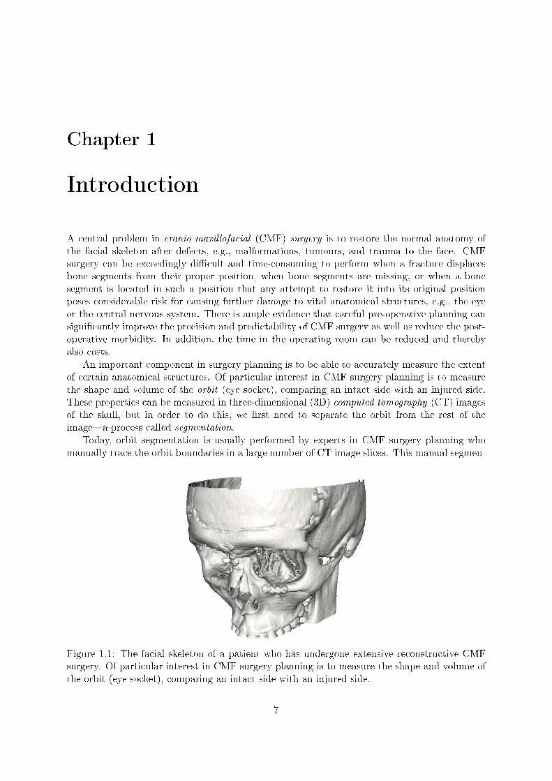
A central problem in cranio-maxillofacial (CMF) surgery is to restore the normal anatomy ofthe facial skeleton after defects, e.g., malformations, tumours, and trauma to the face. CMFsurgery can be exceedingly di�cult and time-consuming to perform when a fracture displacesbone segments from their proper position, when bone segments are missing, or when a bonesegment is located in such a position that any attempt to restore it into its original positionposes considerable risk for causing further damage to vital anatomical structures, e.g., the eyeor the central nervous system. There is ample evidence that careful pre-operative planning cansigni�cantly improve the precision and predictability of CMF surgery as well as reduce the post-operative morbidity. In addition, the time in the operating room can be reduced and therebyalso costs.

An important component in surgery planning is to be able to accurately measure the extentof certain anatomical structures. Of particular interest in CMF surgery planning is to measurethe shape and volume of the orbit (eye socket), comparing an intact side with an injured side.These properties can be measured in three-dimensional (3D) computed tomography (CT) imagesof the skull, but in order to do this, we �rst need to separate the orbit from the rest of theimage�a process called segmentation.

Today, orbit segmentation is usually performed by experts in CMF surgery planning whomanually trace the orbit boundaries in a large number of CT image slices. This manual segmen-

Figure 1.1: The facial skeleton of a patient who has undergone extensive reconstructive CMFsurgery. Of particular interest in CMF surgery planning is to measure the shape and volume ofthe orbit (eye socket), comparing an intact side with an injured side.

7

tation method is accurate but time-consuming, tedious, and sensitive to operator errors. Fullyautomatic orbit segmentation, on the other hand, is unreliable and di�cult to achieve, mainlybecause of the high shape variability of the orbit, the thin nature of the orbital walls, the lack ofan exact de�nition of the orbital opening, and the presence of CT imaging artifacts such as noiseand the partial volume e�ect (PVE). The PVE [1], in particular, can be a major confoundingfactor in orbit segmentation since it transforms parts of the thin bone structures in the orbitinto soft-tissue-like structures.

Image segmentation can be divided into two related tasks: recognition and delineation [2].Recognition is the task of determining where in the image the object of interest is located,whereas delineation is the task of determining the spatial extent of the object. In general,humans outperform computers at the task of recognition, whereas computers are better atdelineation. Previous work on medical image segmentation by, e.g., Vidholm et al. [3] hasshown that the use of semi-automatic or interactive segmentation methods, in which a humanuser provides expert knowledge to the segmentation algorithm through interaction, can lead toincreased segmentation accuracy and reduced user interaction time.

To visualize a 3D CT image on a planar display, e.g., a standard TFT-LCD monitor, we needto create a 2D projection of the 3D data. Advanced volume visualization techniques, combinedwith today's powerful 3D graphics hardware and computer systems, allow us to perform suchprojections at real-time or interactive speeds [2, 4]. Furthermore, when we interact with real-life3D objects, the sense of touch (haptics) is an essential addition to our visual perception. Duringthe last two decades, the development of haptic devices and haptic rendering algorithms has madeit possible to create haptic interfaces in which the user can feel, touch, and manipulate virtual3D objects in a natural and intuitive way. It has been demonstrated [3] that such interfacesgreatly facilitate interactive segmentation of objects in medical volume images.

In this master's thesis project, we develop a prototype of a semi-automatic system for seg-menting orbits in CT images. The system �rst extracts the boundaries of the orbital bonestructures and then segments the orbit by �tting an interactive deformable simplex mesh tothe extracted boundaries. A graphical user interface (GUI) with volume visualization tools andhaptic feedback allows the user to explore the input CT image, de�ne anatomical landmarks,and guide the deformable simplex mesh through the segmentation. We develop the segmentationsystem as an extension of WISH [3, 5], an existing open source software toolkit for interactivesegmentation with haptic interaction. To evaluate the performance of our segmentation system,we let three test users independently segment 14 orbits twice (in a set of seven CT images) withthe segmentation tools provided by the system. For comparison, we also let the three test userssegment the 14 orbits manually.

The project has been carried out at the Centre for Image Analysis (CBA), Uppsala University,Sweden, in cooperation with the Department of Surgical Sciences, Oral & Maxillofacial Surgery,Uppsala University, Sweden.

8

Chapter 2

Digital images

A gray-scale image captured by a sensor can be expressed as a continuous function f(x), wherex is a spatial coordinate vector, and f(x) is the intensity value at x. In order to be processedby a computer, this continuous image function must �rst be digitized, i.e., converted into digitalform [6]. Digitization involves two processes: sampling and quantization. Sampling is the processof taking samples of the continuous image at discrete points in some prede�ned grid, whereasquantization is the process of converting the continuous intensity values of the samples intodiscrete quantities. In the resulting digital image, each image element is a grid point representedby a certain number of bits. A digital image using b storage bits per image element has L = 2b

possible intensity levels (gray-levels). Digital images with only two intensity levels are known asbinary images.

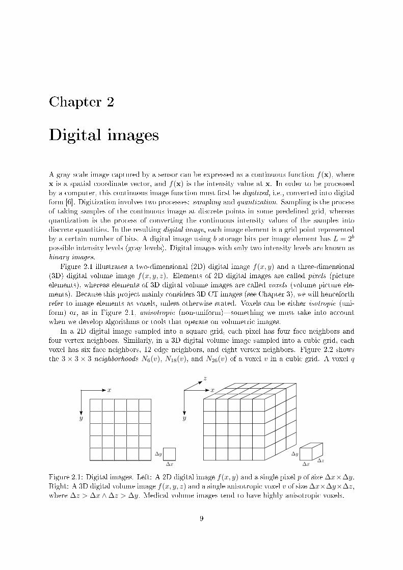
Figure 2.1 illustrates a two-dimensional (2D) digital image f(x, y) and a three-dimensional(3D) digital volume image f(x, y, z). Elements of 2D digital images are called pixels (pictureelements), whereas elements of 3D digital volume images are called voxels (volume picture ele-ments). Because this project mainly considers 3D CT images (see Chapter 3), we will henceforthrefer to image elements as voxels, unless otherwise stated. Voxels can be either isotropic (uni-form) or, as in Figure 2.1, anisotropic (non-uniform)�something we must take into accountwhen we develop algorithms or tools that operate on volumetric images.

In a 2D digital image sampled into a square grid, each pixel has four face neighbors andfour vertex neighbors. Similarly, in a 3D digital volume image sampled into a cubic grid, eachvoxel has six face neighbors, 12 edge neighbors, and eight vertex neighbors. Figure 2.2 showsthe 3 × 3 × 3 neighborhoods N6(v), N18(v), and N26(v) of a voxel v in a cubic grid. A voxel q

Figure 2.1: Digital images. Left: A 2D digital image f(x, y) and a single pixel p of size ∆x×∆y.Right: A 3D digital volume image f(x, y, z) and a single anisotropic voxel v of size ∆x×∆y×∆z,where ∆z > ∆x ∧∆z > ∆y. Medical volume images tend to have highly anisotropic voxels.

9

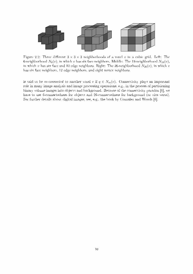
Figure 2.2: Three di�erent 3 × 3 × 3 neighborhoods of a voxel v in a cubic grid. Left: The6-neighborhood N6(v), in which v has six face neighbors. Middle: The 18-neighborhood N18(v),in which v has six face and 12 edge neighbors. Right: The 26-neighborhood N26(v), in which vhas six face neighbors, 12 edge neighbors, and eight vertex neighbors.

is said to be m-connected to another voxel v if q ∈ Nm(v). Connectivity plays an importantrole in many image analysis and image processing operations, e.g., in the process of partitioningbinary volume images into objects and background. Because of the connectivity paradox [6], wehave to use 6-connectedness for objects and 26-connectedness for background (or vice versa).For further details about digital images, see, e.g., the book by Gonzalez and Woods [6].

10

Chapter 3

Computed tomography

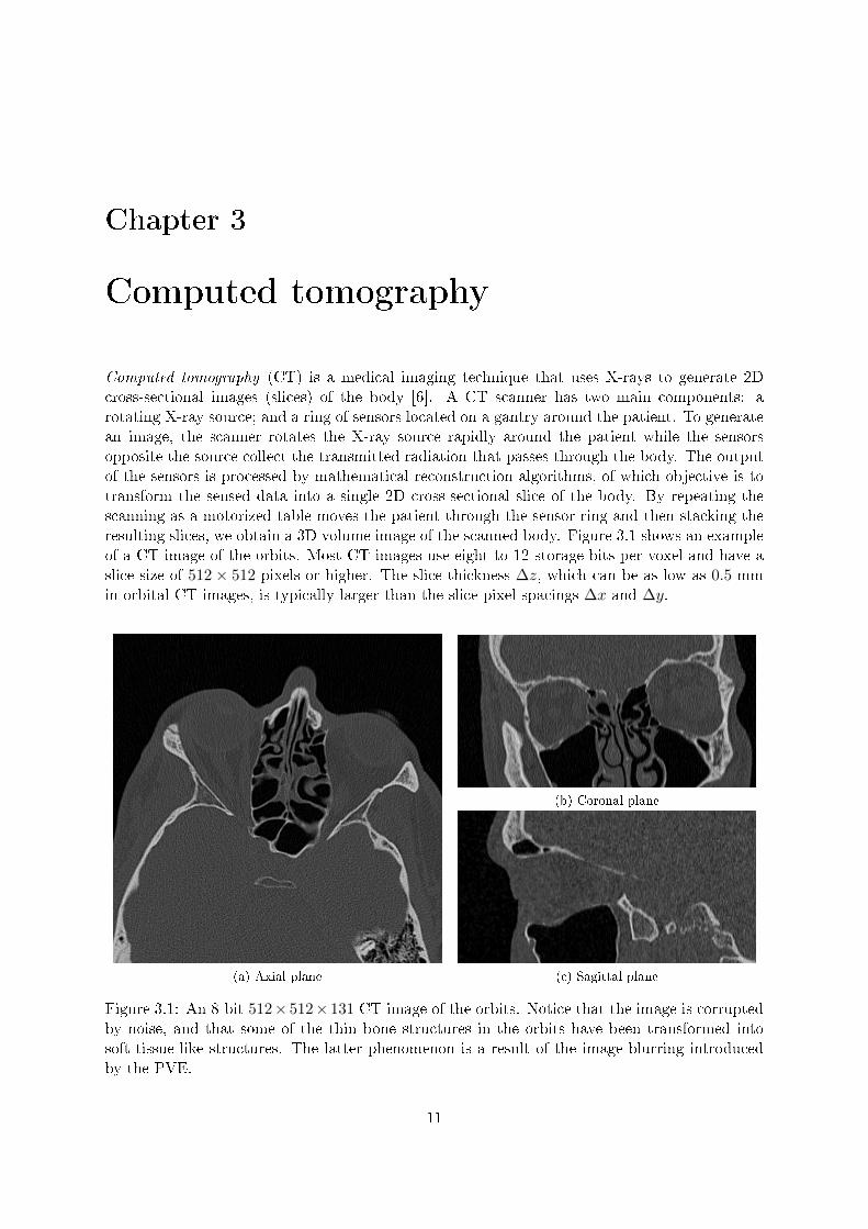
Computed tomography (CT) is a medical imaging technique that uses X-rays to generate 2Dcross-sectional images (slices) of the body [6]. A CT scanner has two main components: arotating X-ray source; and a ring of sensors located on a gantry around the patient. To generatean image, the scanner rotates the X-ray source rapidly around the patient while the sensorsopposite the source collect the transmitted radiation that passes through the body. The outputof the sensors is processed by mathematical reconstruction algorithms, of which objective is totransform the sensed data into a single 2D cross-sectional slice of the body. By repeating thescanning as a motorized table moves the patient through the sensor ring and then stacking theresulting slices, we obtain a 3D volume image of the scanned body. Figure 3.1 shows an exampleof a CT image of the orbits. Most CT images use eight to 12 storage bits per voxel and have aslice size of 512× 512 pixels or higher. The slice thickness ∆z, which can be as low as 0.5 mmin orbital CT images, is typically larger than the slice pixel spacings ∆x and ∆y.

(a) Axial plane

(b) Coronal plane

(c) Sagittal plane

Figure 3.1: An 8-bit 512×512×131 CT image of the orbits. Notice that the image is corruptedby noise, and that some of the thin bone structures in the orbits have been transformed intosoft-tissue-like structures. The latter phenomenon is a result of the image blurring introducedby the PVE.

11

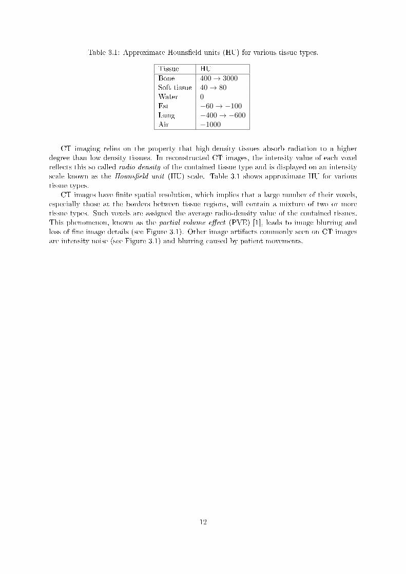
Table 3.1: Approximate Houns�eld units (HU) for various tissue types.

Tissue HU

Bone 400→ 3000Soft tissue 40→ 80Water 0Fat −60→ −100Lung −400→ −600Air −1000

CT imaging relies on the property that high-density tissues absorb radiation to a higherdegree than low-density tissues. In reconstructed CT images, the intensity value of each voxelre�ects this so-called radio-density of the contained tissue type and is displayed on an intensityscale known as the Houns�eld unit (HU) scale. Table 3.1 shows approximate HU for varioustissue types.

CT images have �nite spatial resolution, which implies that a large number of their voxels,especially those at the borders between tissue regions, will contain a mixture of two or moretissue types. Such voxels are assigned the average radio-density value of the contained tissues.This phenomenon, known as the partial volume e�ect (PVE) [1], leads to image blurring andloss of �ne image details (see Figure 3.1). Other image artifacts commonly seen on CT imagesare intensity noise (see Figure 3.1) and blurring caused by patient movements.

12

Chapter 4

Image pre-processing

Image pre-processing operations are used to suppress unwanted image features or enhance certainimage features for further processing [7]. It should be emphasized that image pre-processingoperations never increase the amount of information in the input image; however, they mightremove relevant information and should therefore be used restrictively.

One of the fundamental tools for image pre-processing is spatial �ltering [6]. A spatial �lter

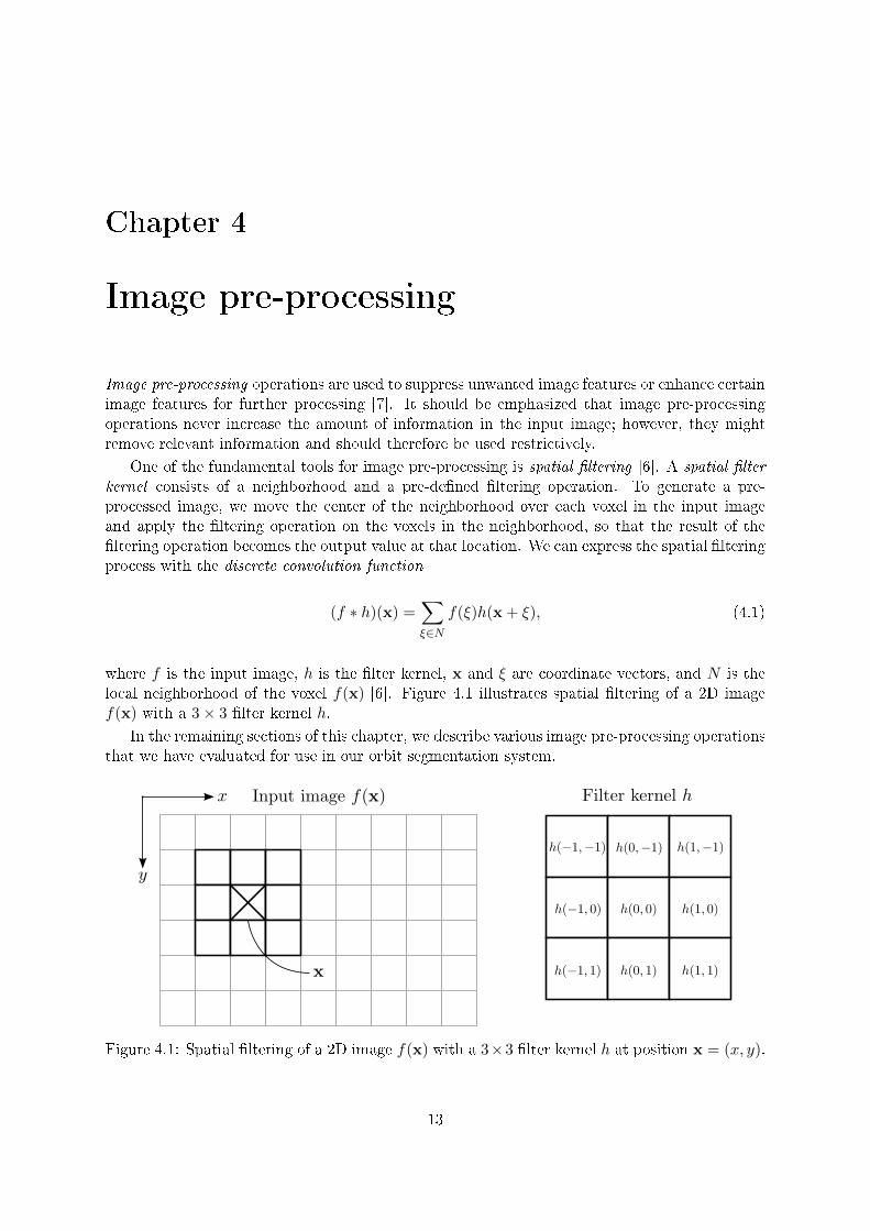
kernel consists of a neighborhood and a pre-de�ned �ltering operation. To generate a pre-processed image, we move the center of the neighborhood over each voxel in the input imageand apply the �ltering operation on the voxels in the neighborhood, so that the result of the�ltering operation becomes the output value at that location. We can express the spatial �lteringprocess with the discrete convolution function

(f ∗ h)(x) =∑ξ∈N

f(ξ)h(x + ξ), (4.1)

where f is the input image, h is the �lter kernel, x and ξ are coordinate vectors, and N is thelocal neighborhood of the voxel f(x) [6]. Figure 4.1 illustrates spatial �ltering of a 2D imagef(x) with a 3× 3 �lter kernel h.

In the remaining sections of this chapter, we describe various image pre-processing operationsthat we have evaluated for use in our orbit segmentation system.

Figure 4.1: Spatial �ltering of a 2D image f(x) with a 3×3 �lter kernel h at position x = (x, y).

13

(a) (b) (c)

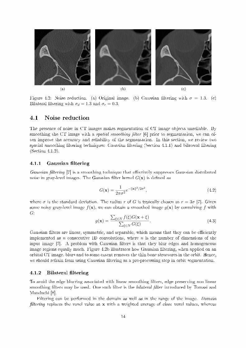
Figure 4.2: Noise reduction. (a) Original image. (b) Gaussian �ltering with σ = 1.3. (c)Bilateral �ltering with σd = 1.3 and σr = 0.3.

4.1 Noise reduction

The presence of noise in CT images makes segmentation of CT image objects unreliable. Bysmoothing the CT image with a spatial smoothing �lter [6] prior to segmentation, we can of-ten improve the accuracy and reliability of the segmentation. In this section, we review twospatial smoothing �ltering techniques: Gaussian �ltering (Section 4.1.1) and bilateral �ltering(Section 4.1.2).

4.1.1 Gaussian �ltering

Gaussian �ltering [7] is a smoothing technique that e�ectively suppresses Gaussian distributednoise in gray-level images. The Gaussian �lter kernel G(x) is de�ned as

G(x) =1

2πσ2e−‖x‖

2/2σ2, (4.2)

where σ is the standard deviation. The radius r of G is typically chosen as r = 3σ [7]. Givensome noisy gray-level image f(x), we can obtain a smoothed image g(x) by convolving f withG:

g(x) =

∑ξ∈N f(ξ)G(x + ξ)∑

ξ∈N G(ξ). (4.3)

Gaussian �lters are linear, symmetric, and separable, which means that they can be e�cientlyimplemented as n consecutive 1D convolutions, where n is the number of dimensions of theinput image [7]. A problem with Gaussian �lters is that they blur edges and homogeneousimage regions equally much. Figure 4.2b illustrates how Gaussian �ltering, when applied on anorbital CT image, blurs and to some extent removes the thin bone structures in the orbit. Hence,we should refrain from using Gaussian �ltering as a pre-processing step in orbit segmentation.

4.1.2 Bilateral �ltering

To avoid the edge blurring associated with linear smoothing �lters, edge preserving non-linearsmoothing �lters may be used. One such �lter is the bilateral �lter introduced by Tomasi andManduchi [8].

Filtering can be performed in the domain as well as in the range of the image. Domain

�ltering replaces the voxel value at x with a weighted average of close voxel values, whereas

14

range �ltering replaces the voxel value at x with a weighted average of similar voxel values.Here, voxels are referred to as being close to each other if they occupy nearby spatial locationsand similar to each other if they have nearby intensity values. The idea of bilateral �ltering isto combine domain and range �ltering, so that the voxel value at x is replaced by a weightedaverage of close and similar voxel values. Bilateral �ltering of a gray-level image f(x) producesa smoothed image h(x), de�ned as

h(x) =

∑ξ∈N f(ξ)c(ξ,x)s(f(ξ), f(x))∑ξ∈N c(ξ,x)s(f(ξ), f(x))

, (4.4)

where c(ξ,x) is the closeness function

c(ξ,x) =1

2πσ2d

e−‖ξ−x‖2/2σ2

d , (4.5)

and s(f(ξ), f(x)) is the similarity function

s(f(ξ), f(x)) =1

2πσ2e−‖f(ξ)−f(x)‖2/2σ2

r . (4.6)

Other de�nitions of the closeness and similarity functions are also possible [8]. The geometric

spread σd in the image domain is chosen based on the desired amount of smoothing we want toachieve in homogeneous image regions, whereas the photometric spread σr in the image range ischosen to achieve the desired amount of combination of voxel values [8]. If ‖f(ξ)− f(x)‖ � σr,then f(ξ) and f(x) will be mixed together, otherwise not.

Bilateral �lters are non-linear and non-separable and are therefore slower and more expensiveto compute than Gaussian �lters of corresponding size. The main advantage of using bilateral�lters is that they smooth homogeneous image regions while preserving edges (as shown inFigure 4.2c). Thus, bilateral �ltering should be a suitable method for suppressing noise inorbital CT images.

4.2 Image sharpening

Spatial sharpening �lters are used to enhance edges in images [6]. A spatial sharpening �lterthat has become the standard sharpening tool in many digital image processing systems is theunsharp mask �lter [6]. This �lter e�ectively sharpens edges without overly amplifying noise [9]and might therefore be a suitable tool for sharpening orbital CT images.

The idea of unsharp masking is to �rst blur the original image f(x) with a spatial smoothing�lter (e.g., a Gaussian �lter of scale σ) and then subtract the blurred image from f to createan unsharp mask. By adding this mask, multiplied with a positive weight k, to f , we obtain asharpened version of f .

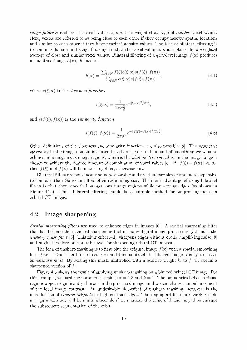
Figure 4.3 shows the result of applying unsharp masking on a blurred orbital CT image. Forthis example, we used the parameter settings σ = 1.3 and k = 1. The boundaries between tissueregions appear signi�cantly sharper in the processed image, and we can also see an enhancementof the local image contrast. An undesirable side-e�ect of unsharp masking, however, is theintroduction of ringing artifacts at high-contrast edges. The ringing artifacts are barely visiblein Figure 4.3b but will be more noticeable if we increase the value of k and may then corruptthe subsequent segmentation of the orbit.

15

(a) (b)

Figure 4.3: Image sharpening. (a) Original image. (b) Unsharp masking with σ = 1.3 andk = 1.

4.3 Edge detection

An edge in a digital image is a pixel or voxel in which the image intensity function changesabruptly. Image pre-processing methods used to locate such abrupt intensity changes are callededge detectors [7]. To determine edge direction and strength, many edge detectors use approxi-mations of the image gradient and the image gradient magnitude, respectively. In this section, wedescribe some standard gradient approximation methods (Section 4.3.1) and provide an exampleof a 3D edge detector (Section 4.3.2).

4.3.1 Gradient approximation

For a continuous 3D function f(x), the gradient of f at the coordinate x = (x, y, z) is de�nedas

∇f(x) =

gxgygz

=

∂f∂x∂f∂y∂f∂z

. (4.7)

For a digital volume image f(x), we cannot compute ∇f analytically. We can, however, approx-imate ∇f by using, e.g., the centered di�erence formula

∇f(x) =

gxgygz

≈f(x+1,y,z)−f(x−1,y,z)

2∆xf(x,y+1,z)−f(x,y+1,z)

2∆yf(x,y,z+1)−f(x,y,z+1)

2∆z

. (4.8)

The gradient magnitude ‖∇f(x)‖ represents the rate of change in the direction of the gradientvector and is de�ned as

‖∇f(x)‖ =√g2x + g2

y + g2z . (4.9)

Linear gradient �lters based on �nite di�erence approximations respond strongly to noise; thus,to obtain reliable gradient approximations, we have to incorporate noise reduction in the gradientcomputation [7]. A simple but rather ine�cient way to achieve this is to �rst smooth the inputimage f with a Gaussian �lter G and then compute the gradient of the smoothed image [7]. Amore e�cient way is to use a Gaussian gradient �lter [7]. Because convolution is associative andcommutative, the gradient of f can be e�ciently computed by convolving f with the gradientof G:

∇[G(x) ∗ f(x)] = [∇G(x)] ∗ f(x) (4.10)

16

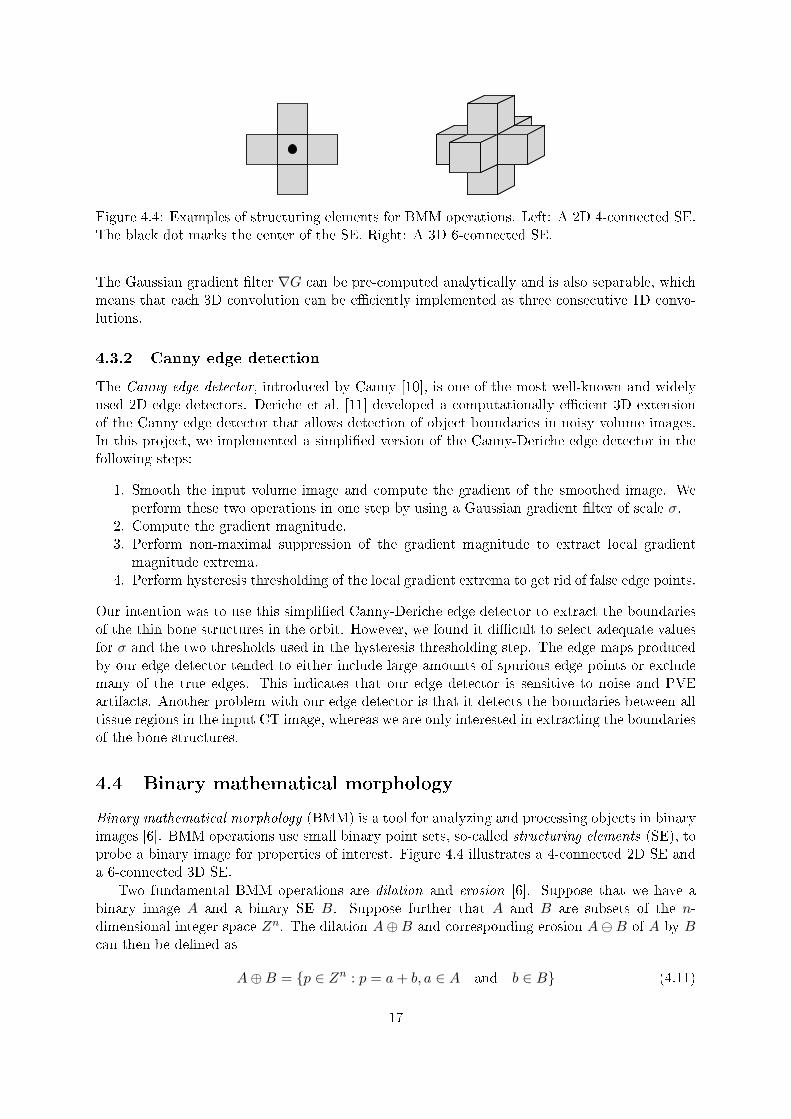
Figure 4.4: Examples of structuring elements for BMM operations. Left: A 2D 4-connected SE.The black dot marks the center of the SE. Right: A 3D 6-connected SE.

The Gaussian gradient �lter ∇G can be pre-computed analytically and is also separable, whichmeans that each 3D convolution can be e�ciently implemented as three consecutive 1D convo-lutions.

4.3.2 Canny edge detection

The Canny edge detector, introduced by Canny [10], is one of the most well-known and widelyused 2D edge detectors. Deriche et al. [11] developed a computationally e�cient 3D extensionof the Canny edge detector that allows detection of object boundaries in noisy volume images.In this project, we implemented a simpli�ed version of the Canny-Deriche edge detector in thefollowing steps:

1. Smooth the input volume image and compute the gradient of the smoothed image. Weperform these two operations in one step by using a Gaussian gradient �lter of scale σ.

2. Compute the gradient magnitude.3. Perform non-maximal suppression of the gradient magnitude to extract local gradient

magnitude extrema.4. Perform hysteresis thresholding of the local gradient extrema to get rid of false edge points.

Our intention was to use this simpli�ed Canny-Deriche edge detector to extract the boundariesof the thin bone structures in the orbit. However, we found it di�cult to select adequate valuesfor σ and the two thresholds used in the hysteresis thresholding step. The edge maps producedby our edge detector tended to either include large amounts of spurious edge points or excludemany of the true edges. This indicates that our edge detector is sensitive to noise and PVEartifacts. Another problem with our edge detector is that it detects the boundaries between alltissue regions in the input CT image, whereas we are only interested in extracting the boundariesof the bone structures.

4.4 Binary mathematical morphology

Binary mathematical morphology (BMM) is a tool for analyzing and processing objects in binaryimages [6]. BMM operations use small binary point sets, so-called structuring elements (SE), toprobe a binary image for properties of interest. Figure 4.4 illustrates a 4-connected 2D SE anda 6-connected 3D SE.

Two fundamental BMM operations are dilation and erosion [6]. Suppose that we have abinary image A and a binary SE B. Suppose further that A and B are subsets of the n-dimensional integer space Zn. The dilation A⊕B and corresponding erosion AB of A by Bcan then be de�ned as

A⊕B = {p ∈ Zn : p = a+ b, a ∈ A and b ∈ B} (4.11)

17

(a) (b) (c)

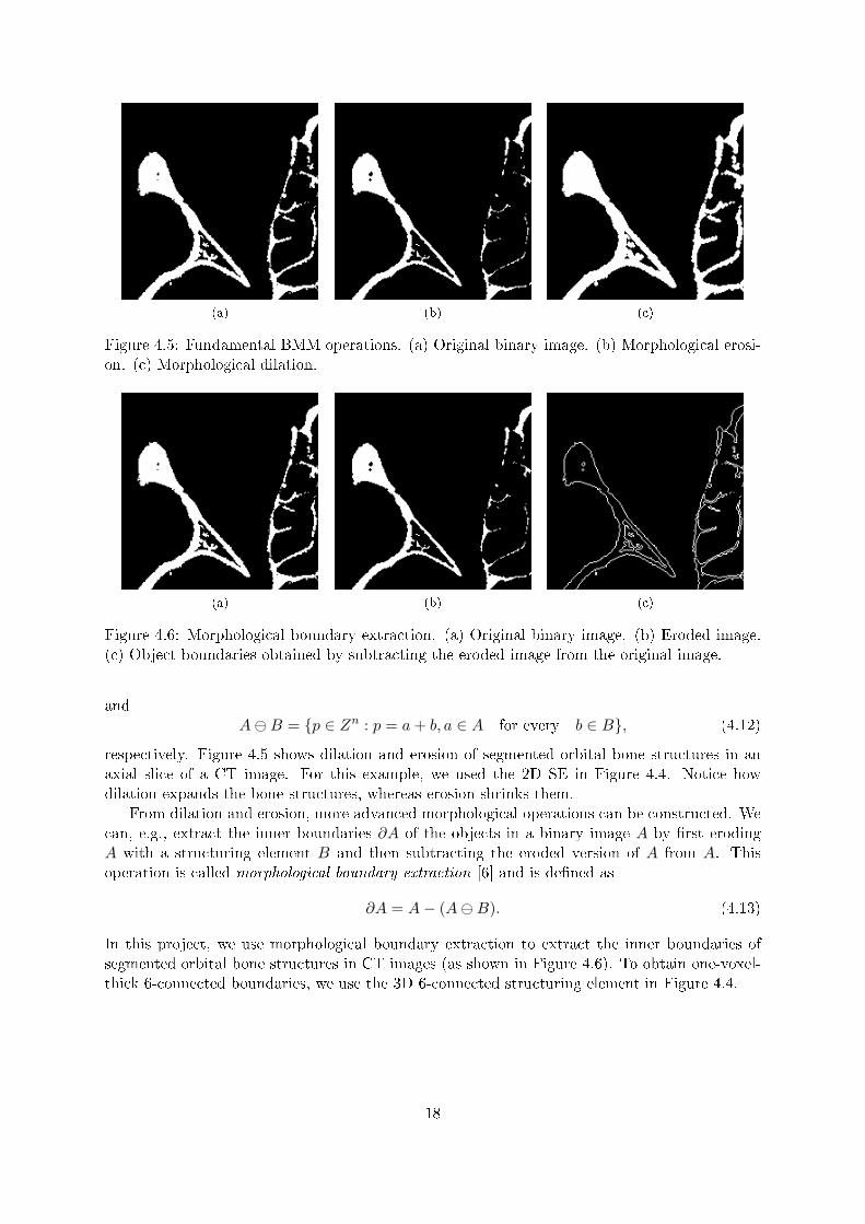
Figure 4.5: Fundamental BMM operations. (a) Original binary image. (b) Morphological erosi-on. (c) Morphological dilation.

(a) (b) (c)

Figure 4.6: Morphological boundary extraction. (a) Original binary image. (b) Eroded image.(c) Object boundaries obtained by subtracting the eroded image from the original image.

andAB = {p ∈ Zn : p = a+ b, a ∈ A for every b ∈ B}, (4.12)

respectively. Figure 4.5 shows dilation and erosion of segmented orbital bone structures in anaxial slice of a CT image. For this example, we used the 2D SE in Figure 4.4. Notice howdilation expands the bone structures, whereas erosion shrinks them.

From dilation and erosion, more advanced morphological operations can be constructed. Wecan, e.g., extract the inner boundaries ∂A of the objects in a binary image A by �rst erodingA with a structuring element B and then subtracting the eroded version of A from A. Thisoperation is called morphological boundary extraction [6] and is de�ned as

∂A = A− (AB). (4.13)

In this project, we use morphological boundary extraction to extract the inner boundaries ofsegmented orbital bone structures in CT images (as shown in Figure 4.6). To obtain one-voxel-thick 6-connected boundaries, we use the 3D 6-connected structuring element in Figure 4.4.

18

Chapter 5

Image segmentation

Image segmentation, the process of identifying and separating objects of interest from the restof the image, is a fundamental problem in medical image analysis, where accurate segmentationusually is a pre-requisite for further analysis of image objects. Despite decades of research, fullyautomatic segmentation of arbitrary medical images is still an unsolved problem [3]. Manualsegmentation, on the other hand, is often too time-consuming, tedious, and sensitive to usererrors to be of practical use.

In this chapter, we investigate the usefulness of semi-automatic or interactive segmentationmethods in segmenting orbits or orbital bone structures in CT images. We review four seg-mentation methods: global thresholding (Section 5.1.1), hysteresis thresholding (Section 5.1.2),multi-seeded fuzzy connectedness segmentation (Section 5.2), and deformable simplex mesh seg-mentation (Section 5.3). At the end of the chapter, we propose a semi-automatic method fororbit segmentation (Section 5.4).

5.1 Gray-level thresholding

The underlying idea of gray-level thresholding is that gray-level images can be directly partitionedinto regions based on intensity values [6]. This section focuses on two common thresholdingmethods: global thresholding (Section 5.1.1) and hysteresis thresholding (Section 5.1.2).

5.1.1 Global thresholding

Global thresholding [6] is one of the simplest and most widely used segmentation methods.Given a gray-scale volume image f(x) composed of bright objects on a dark background (or viceversa), we select a single gray-level t (the global threshold) that separates the objects from thebackground and threshold f at t to generate a segmented binary image g(x), de�ned as

g(x) =

{1 if f(x) ≥ t0 otherwise

, (5.1)

where g(x) = 1 are the object voxels and g(x) = 0 are the background voxels.A threshold that separates two image regions from each other is usually located in an obvious

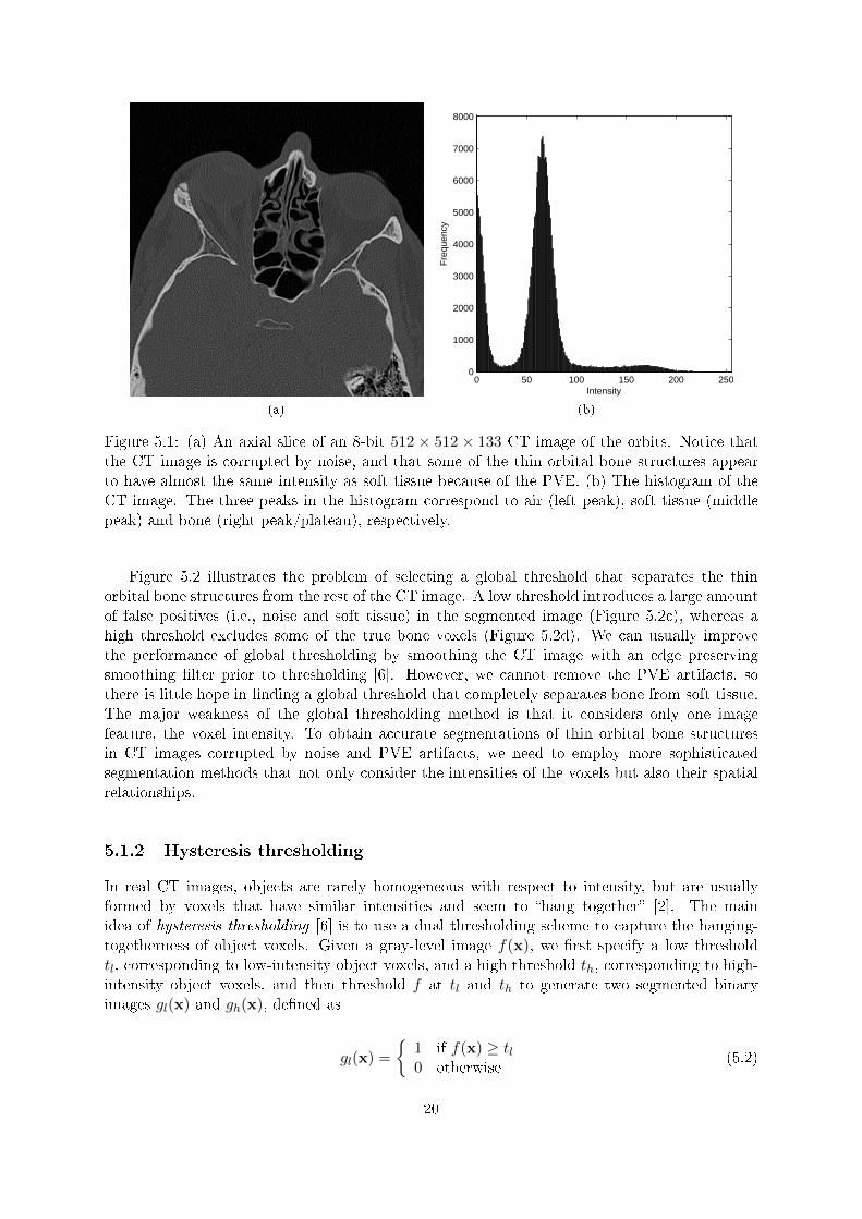
and deep valley of the image histogram. Figure 5.1a shows an axial slice of an 8-bit 512×512×133CT image of the orbits. The histogram of this CT image (Figure 5.1b) shows three peaks,corresponding to air (left peak), soft tissue (middle peak) and bone tissue (right peak/plateau).Due to noise and PVE artifacts, there is no distinct valley between the middle peak and theright peak in the histogram. Thus, we cannot easily separate bone and soft tissue with a singleglobal threshold.

19

(a)

0 50 100 150 200 2500

1000

2000

3000

4000

5000

6000

7000

8000

Intensity

Fre

quen

cy

(b)

Figure 5.1: (a) An axial slice of an 8-bit 512 × 512 × 133 CT image of the orbits. Notice thatthe CT image is corrupted by noise, and that some of the thin orbital bone structures appearto have almost the same intensity as soft tissue because of the PVE. (b) The histogram of theCT image. The three peaks in the histogram correspond to air (left peak), soft tissue (middlepeak) and bone (right peak/plateau), respectively.

Figure 5.2 illustrates the problem of selecting a global threshold that separates the thinorbital bone structures from the rest of the CT image. A low threshold introduces a large amountof false positives (i.e., noise and soft tissue) in the segmented image (Figure 5.2c), whereas ahigh threshold excludes some of the true bone voxels (Figure 5.2d). We can usually improvethe performance of global thresholding by smoothing the CT image with an edge preservingsmoothing �lter prior to thresholding [6]. However, we cannot remove the PVE artifacts, sothere is little hope in �nding a global threshold that completely separates bone from soft tissue.The major weakness of the global thresholding method is that it considers only one imagefeature, the voxel intensity. To obtain accurate segmentations of thin orbital bone structuresin CT images corrupted by noise and PVE artifacts, we need to employ more sophisticatedsegmentation methods that not only consider the intensities of the voxels but also their spatialrelationships.

5.1.2 Hysteresis thresholding

In real CT images, objects are rarely homogeneous with respect to intensity, but are usuallyformed by voxels that have similar intensities and seem to �hang together� [2]. The mainidea of hysteresis thresholding [6] is to use a dual thresholding scheme to capture the hanging-togetherness of object voxels. Given a gray-level image f(x), we �rst specify a low thresholdtl, corresponding to low-intensity object voxels, and a high threshold th, corresponding to high-intensity object voxels, and then threshold f at tl and th to generate two segmented binaryimages gl(x) and gh(x), de�ned as

gl(x) =

{1 if f(x) ≥ tl0 otherwise

(5.2)

20

(a) (b) (c)

(d) (e) (f)

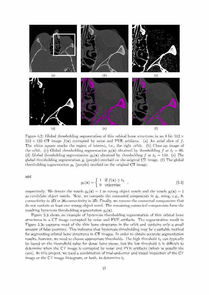
Figure 5.2: Global thresholding segmentation of thin orbital bone structures in an 8-bit 512 ×512 × 133 CT image f(x) corrupted by noise and PVE artifacts. (a) An axial slice of f .The white square marks the region of interest, i.e., the right orbit. (b) Close-up image ofthe orbit. (c) Global thresholding segmentation gl(x) obtained by thresholding f at tl = 80.(d) Global thresholding segmentation gh(x) obtained by thresholding f at th = 110. (e) Theglobal thresholding segmentation gl (purple) overlaid on the original CT image. (f) The globalthresholding segmentation gh (purple) overlaid on the original CT image.

and

gh(x) =

{1 if f(x) ≥ th0 otherwise

, (5.3)

respectively. We denote the voxels gh(x) = 1 as strong object voxels and the voxels gl(x) = 1as candidate object voxels. Next, we compute the connected components in gl, using, e.g., 8-connectivity in 2D or 26-connectivity in 3D. Finally, we remove the connected components thatdo not contain at least one strong object voxel. The remaining connected components form theresulting hysteresis thresholding segmentation gs(x).

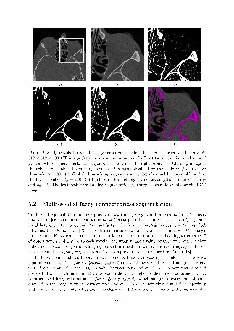
Figure 5.3 shows an example of hysteresis thresholding segmentation of thin orbital bonestructures in a CT image corrupted by noise and PVE artifacts. The segmentation result inFigure 5.3e captures most of the thin bone structures in the orbit and contains only a smallamount of false positives. This indicates that hysteresis thresholding may be a suitable methodfor segmenting orbital bone structures in CT images. In order to obtain accurate segmentationresults, however, we need to choose appropriate thresholds. The high threshold th can typicallybe based on the Houns�eld value for dense bone tissue, but the low threshold tl is di�cult todetermine when the CT image is corrupted by noise and PVE artifacts (which is usually thecase). In this project, we used a combination of trial-and-error and visual inspection of the CTimage or the CT image histogram, or both, to determine tl.

21

(a) (b) (c)

(d) (e) (f)

Figure 5.3: Hysteresis thresholding segmentation of thin orbital bone structures in an 8-bit512 × 512 × 133 CT image f(x) corrupted by noise and PVE artifacts. (a) An axial slice off . The white square marks the region of interest, i.e., the right orbit. (b) Close-up image ofthe orbit. (c) Global thresholding segmentation gl(x) obtained by thresholding f at the lowthreshold tl = 80. (d) Global thresholding segmentation gh(x) obtained by thresholding f atthe high threshold th = 110. (e) Hysteresis thresholding segmentation gs(x) obtained from gland gh. (f) The hysteresis thresholding segmentation gs (purple) overlaid on the original CTimage.

5.2 Multi-seeded fuzzy connectedness segmentation

Traditional segmentation methods produce crisp (binary) segmentation results. In CT images,however, object boundaries tend to be fuzzy (unsharp) rather than crisp because of, e.g., ma-terial heterogeneity, noise, and PVE artifacts. The fuzzy connectedness segmentation method,introduced by Udupa et al. [12], takes these intrinsic uncertainties and inaccuracies of CT imagesinto account. Fuzzy connectedness segmentation attempts to capture the �hanging-togetherness�of object voxels and assigns to each voxel in the input image a value between zero and one thatindicates the voxel's degree of belongingness to the object of interest. The resulting segmentationis represented as a fuzzy set, an alternative set representation introduced by Zadeh [13].

In fuzzy connectedness theory, image elements (pixels or voxels) are referred to as spels

(spatial elements). The fuzzy adjacency µα(c, d) is a local fuzzy relation that assigns to everypair of spels c and d in the image a value between zero and one based on how close c and dare spatially. The closer c and d are to each other, the higher is their fuzzy adjacency value.Another local fuzzy relation is the fuzzy a�nity µκ(c, d), which assigns to every pair of spelsc and d in the image a value between zero and one based on how close c and d are spatiallyand how similar their intensities are. The closer c and d are to each other and the more similar

22

their intensities are, the higher is their fuzzy a�nity value. Fuzzy connectedness is a globalfuzzy relation that assigns to every pair of spels in the image a strength of connectedness (globalhanging-togetherness) based on the a�nity values (local hanging-togetherness) found along allpossible paths between the two spels. A path between two spels c and d is a sequence of linksbetween successive spels in the image, starting from c and ending in d. The strength of a linkbetween two successive spels in the path is their a�nity, and the strength of a path is thestrength of its weakest link. The strength of fuzzy connectedness µK(c, d) between a pair ofspels c and d is then the strength of the strongest path between c and d [12].

To segment an image, we �rst specify a seed spel c somewhere inside the object of interestand then compute the strength of fuzzy connectedness between c and every other spel di in theimage, generating a fuzzy connectedness map (i.e., a fuzzy segmentation) in which each voxel hasa value between zero and one that indicates the voxel's degree of belongingness to the object ofinterest. From this fuzzy connectedness map, we can optionally obtain a crisp segmentation bythresholding the fuzzy connectedness map at some level α ∈ [0, 1]�a process known as α-cutting.The process of determining the strengths of all possible paths between c and every other speldi is a problem of high combinatorial complexity, which makes the fuzzy connectedness mappotentially time-consuming to compute [12]. Nyul et al. [14] demonstrated that it is possible tocompute 3D fuzzy connectedness maps at interactive speeds by combining e�cient graph searchalgorithms with modern PC hardware.

The original fuzzy connectedness segmentation method uses a single seed to segment a singleobject in the input image. However, single-seeded fuzzy connectedness segmentation becomesimpractical when the object of interest is composed of several disjoint or seemingly disjointcomponents (as is the case for the orbital bone structures). Moreover, unless the seeding is donemanually, it is often easier to extract a set of seeds from the object of interest than to extractexactly one seed. The multi-seeded fuzzy connectedness segmentation method, introduced bySaha and Udupa [15], solves these problems by allowing the user to specify multiple seeds perobject and perform simultaneous segmentation of multiple disjoint objects.

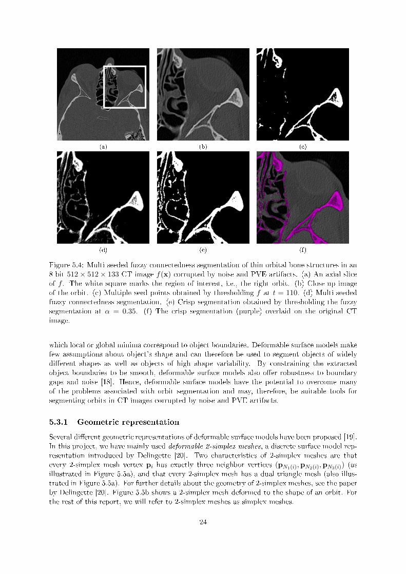
Figure 5.4 shows an example of multi-seeded fuzzy connectedness segmentation of thin orbitalbone structures in a CT image corrupted by noise and PVE artifacts. For this example, wegenerated multiple seeds (Figure 5.4c) by thresholding the CT image at t = 110. The fuzzyconnectedness map (Figure 5.4d) provides an accurate and information-rich representation ofthe bone structures in the image. The crisp segmentation (Figure 5.4e), which we obtainedby thresholding the fuzzy connectedness map at α = 0.35, captures the orbital bone structuresaccurately and contains only a small amount of false positives. Although anecdotal, this exampleindicates that multi-seeded fuzzy connectedness segmentation is robust to noise and PVE.

An advantage of using multi-seeded fuzzy connectedness segmentation over hysteresis thresh-olding is that we do not have to take a crisp (and possible premature) decision about the lowerthreshold for bone tissue. We still have to select a threshold that generates at least one seedinside each bone segment in the orbit, but once we have computed the fuzzy connectednessmap, we can rapidly threshold it at di�erent membership levels α until we obtain a su�cientlyaccurate crisp segmentation.

5.3 Deformable simplex meshes

Deformable contour models (also known as 2D snakes) were introduced by Kass et al. [16] andextended to deformable surface models (also known as 3D snakes) by Terzopoulos et al. [17].Since their introduction in the late 1980s, deformable surface models have been frequently usedin medical image segmentation. A deformable surface model may be thought of as an elasticsurface (de�ned in the image domain) that is driven by the minimization of a cost function, of

23

(a) (b) (c)

(d) (e) (f)

Figure 5.4: Multi-seeded fuzzy connectedness segmentation of thin orbital bone structures in an8-bit 512× 512× 133 CT image f(x) corrupted by noise and PVE artifacts. (a) An axial sliceof f . The white square marks the region of interest, i.e., the right orbit. (b) Close-up imageof the orbit. (c) Multiple seed-points obtained by thresholding f at t = 110. (d) Multi-seededfuzzy connectedness segmentation. (e) Crisp segmentation obtained by thresholding the fuzzysegmentation at α = 0.35. (f) The crisp segmentation (purple) overlaid on the original CTimage.

which local or global minima correspond to object boundaries. Deformable surface models makefew assumptions about object's shape and can therefore be used to segment objects of widelydi�erent shapes as well as objects of high shape variability. By constraining the extractedobject boundaries to be smooth, deformable surface models also o�er robustness to boundarygaps and noise [18]. Hence, deformable surface models have the potential to overcome manyof the problems associated with orbit segmentation and may, therefore, be suitable tools forsegmenting orbits in CT images corrupted by noise and PVE artifacts.

5.3.1 Geometric representation

Several di�erent geometric representations of deformable surface models have been proposed [19].In this project, we have mainly used deformable 2-simplex meshes, a discrete surface model rep-resentation introduced by Delingette [20]. Two characteristics of 2-simplex meshes are thatevery 2-simplex mesh vertex pi has exactly three neighbor vertices (pN1(i),pN2(i),pN3(i)) (asillustrated in Figure 5.5a), and that every 2-simplex mesh has a dual triangle mesh (also illus-trated in Figure 5.5a). For further details about the geometry of 2-simplex meshes, see the paperby Delingette [20]. Figure 5.5b shows a 2-simplex mesh deformed to the shape of an orbit. Forthe rest of this report, we will refer to 2-simplex meshes as simplex meshes.

24

(a) (b)

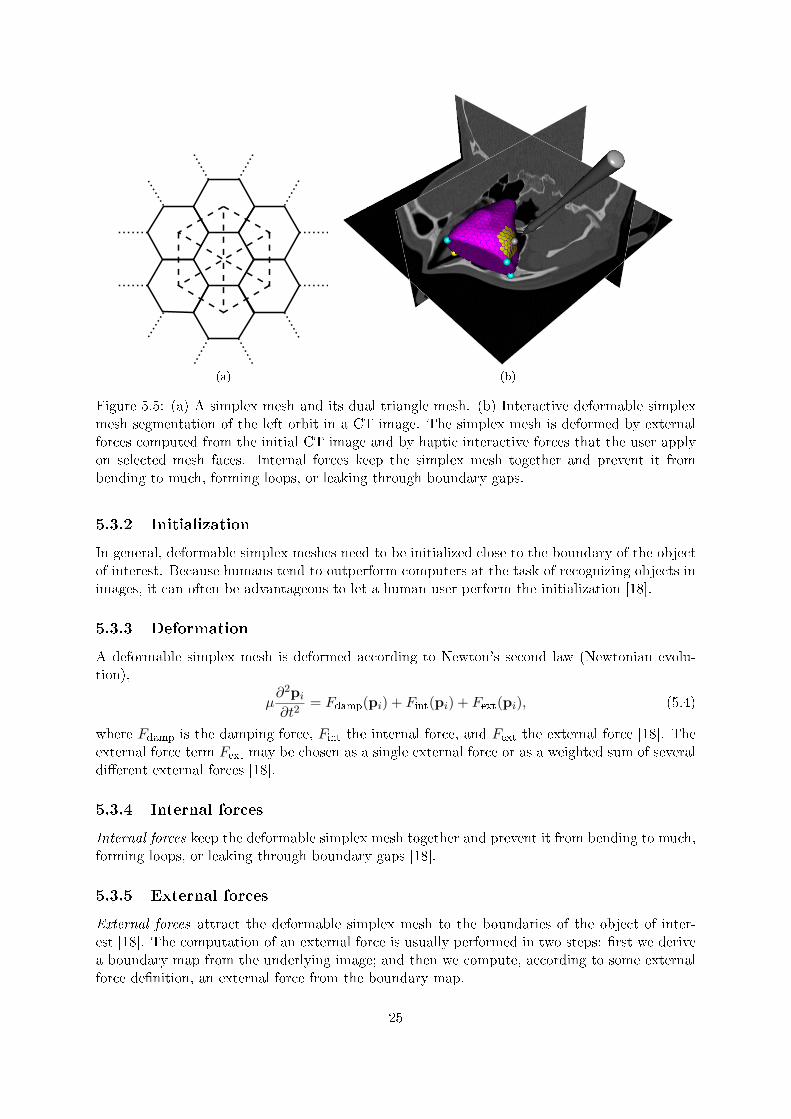
Figure 5.5: (a) A simplex mesh and its dual triangle mesh. (b) Interactive deformable simplexmesh segmentation of the left orbit in a CT image. The simplex mesh is deformed by externalforces computed from the initial CT image and by haptic interactive forces that the user applyon selected mesh faces. Internal forces keep the simplex mesh together and prevent it frombending to much, forming loops, or leaking through boundary gaps.

5.3.2 Initialization

In general, deformable simplex meshes need to be initialized close to the boundary of the objectof interest. Because humans tend to outperform computers at the task of recognizing objects inimages, it can often be advantageous to let a human user perform the initialization [18].

5.3.3 Deformation

A deformable simplex mesh is deformed according to Newton's second law (Newtonian evolu-tion),

µ∂2pi∂t2

= Fdamp(pi) + Fint(pi) + Fext(pi), (5.4)

where Fdamp is the damping force, Fint the internal force, and Fext the external force [18]. Theexternal force term Fext may be chosen as a single external force or as a weighted sum of severaldi�erent external forces [18].

5.3.4 Internal forces

Internal forces keep the deformable simplex mesh together and prevent it from bending to much,forming loops, or leaking through boundary gaps [18].

5.3.5 External forces

External forces attract the deformable simplex mesh to the boundaries of the object of inter-est [18]. The computation of an external force is usually performed in two steps: �rst we derivea boundary map from the underlying image; and then we compute, according to some externalforce de�nition, an external force from the boundary map.

25

(a) (b) (c)

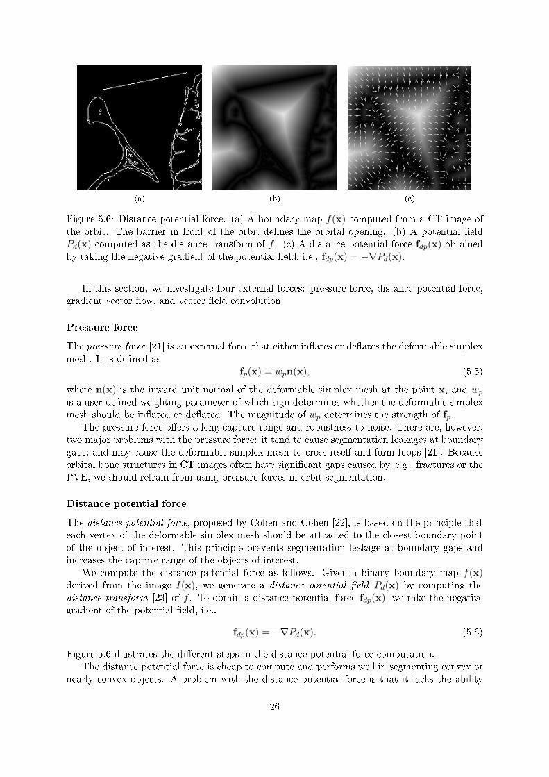
Figure 5.6: Distance potential force. (a) A boundary map f(x) computed from a CT image ofthe orbit. The barrier in front of the orbit de�nes the orbital opening. (b) A potential �eldPd(x) computed as the distance transform of f . (c) A distance potential force fdp(x) obtainedby taking the negative gradient of the potential �eld, i.e., fdp(x) = −∇Pd(x).

In this section, we investigate four external forces: pressure force, distance potential force,gradient vector �ow, and vector �eld convolution.

Pressure force

The pressure force [21] is an external force that either in�ates or de�ates the deformable simplexmesh. It is de�ned as

fp(x) = wpn(x), (5.5)

where n(x) is the inward unit normal of the deformable simplex mesh at the point x, and wpis a user-de�ned weighting parameter of which sign determines whether the deformable simplexmesh should be in�ated or de�ated. The magnitude of wp determines the strength of fp.

The pressure force o�ers a long capture range and robustness to noise. There are, however,two major problems with the pressure force: it tend to cause segmentation leakages at boundarygaps; and may cause the deformable simplex mesh to cross itself and form loops [21]. Becauseorbital bone structures in CT images often have signi�cant gaps caused by, e.g., fractures or thePVE, we should refrain from using pressure forces in orbit segmentation.

Distance potential force

The distance potential force, proposed by Cohen and Cohen [22], is based on the principle thateach vertex of the deformable simplex mesh should be attracted to the closest boundary pointof the object of interest. This principle prevents segmentation leakage at boundary gaps andincreases the capture range of the objects of interest.

We compute the distance potential force as follows. Given a binary boundary map f(x)derived from the image I(x), we generate a distance potential �eld Pd(x) by computing thedistance transform [23] of f . To obtain a distance potential force fdp(x), we take the negativegradient of the potential �eld, i.e.,

fdp(x) = −∇Pd(x). (5.6)

Figure 5.6 illustrates the di�erent steps in the distance potential force computation.The distance potential force is cheap to compute and performs well in segmenting convex or

nearly convex objects. A problem with the distance potential force is that it lacks the ability

26

to deform simplex meshes into narrow boundary concavities; however, most orbits are nearlyconvex, so the distance potential force should, in most cases, be able to capture the boundaryof the orbit.

Gradient vector �ow

Gradient vector �ow (GVF) �elds, introduced by Xu and Prince [18], provide a long capturerange, prevent segmentation leakage at boundary gaps, and have the ability to capture narrowboundary concavities. A 3D GVF �eld fgvf(x) minimizes the energy functional

Egvf =

∫R3

µ‖∇fgvf(x)‖2 + ‖∇f(x)‖2‖fgvf(x)−∇f(x)‖2dx, (5.7)

where f is a binary or gray-level boundary map, and µ is a regularization parameter that controlsthe smoothness of the GVF �eld. The �rst term in the integral is responsible for producing asmoothly varying vector �eld in homogeneous regions, whereas the second term forces the GVF�eld to be close to ∇f in regions close to boundaries.

Although well-suited for orbit segmentation, GVF �elds have some disadvantages: they areexpensive to compute; and are sensitive to noise and parameter settings. Computing a 3DGVF �eld with the original GVF algorithm, which uses �nite di�erence approximations and asimple iterative method to solve Equation 5.7 [18], may take several hours. Vidholm et al. [24]demonstrated that multi-grid methods can reduce the computational time from hours to mereminutes, which is an acceptable time for interactive segmentation.

Vector �eld convolution

Vector �eld convolution (VFC) �elds, introduced by Li and Scott [25], have all the desirableproperties of GVF �elds, but are cheaper to compute, more customizable, and less sensitive tonoise and parameter settings. To compute a 3D VFC �eld, we �rst create a vector �eld kernel

k(x) of radius R, de�ned ask(x) = m(x)n(x), (5.8)

where m(x) is a magnitude function, e.g.,

m(x) = (r + ε)−γ , (5.9)

and n(x) is a unit vector that points to the kernel origin, de�ned as

n(x) = −x/r. (5.10)

In Equations 5.9 and 5.10, r is the distance ‖x‖ from the kernel origin, ε is a small positiveconstant used to prevent division by zero, and γ is a positive parameter that controls thedecreasingness of the magnitude function. The 3D VFC �eld fvfc(x) is computed by convolvingk with a binary or gray-level boundary map f(x):

fvfc(x) = f(x) ∗ k(x) (5.11)

The convolution in Equation 5.11 is expensive to compute, but can be accelerated by the fastFourier transform (FFT) [25]. The performance of a VFC �eld depends on the quality of theboundary map, the choice of magnitude function m, and the kernel radius R. By increasing R,we increase the capture range of the VFC �eld, but also make the convolution more expensive tocompute. For the magnitude function de�ned in Equation 5.9, a small γ forces the deformablesimplex mesh to ignore noise and weak object boundaries, whereas a large γ increases thein�uence of object boundaries and noise.

27

5.3.6 Interactive forces

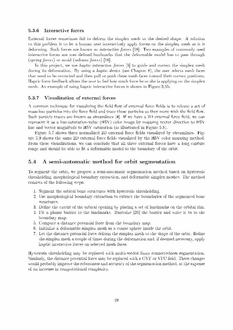
External forces sometimes fail to deform the simplex mesh to the desired shape. A solutionto this problem is to let a human user interactively apply forces on the simplex mesh as it isdeforming. Such forces are known as interactive forces [18]. Two examples of commonly usedinteractive forces are user de�ned landmarks that the deformable model has to pass through(spring forces) or avoid (volcano forces) [18].

In this project, we use haptic interactive forces [3] to guide and correct the simplex meshduring its deformation. By using a haptic device (see Chapter 8), the user selects mesh facesthat need to be corrected and then pull or push these mesh faces toward their correct positions.Haptic force feedback allows the user to feel how much force he or she is applying on the simplexmesh. An example of using haptic interactive forces is shown in Figure 5.5b.

5.3.7 Visualization of external forces

A common technique for visualizing the �eld �ow of external force �elds is to release a set ofmass-less particles into the force �eld and trace these particles as they move with the �eld �ow.Such particle traces are known as streamlines [4]. If we have a 2D external force �eld, we canrepresent it as a hue-saturation-value (HSV) color image by mapping vector direction to HSVhue and vector magnitude to HSV saturation (as illustrated in Figure 5.8).

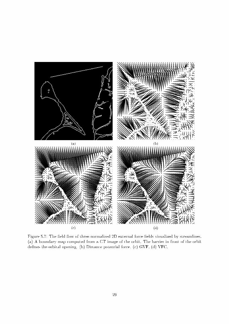
Figure 5.7 shows three normalized 2D external force �elds visualized by streamlines. Fig-ure 5.9 shows the same 2D external force �elds visualized by the HSV color mapping method.From these visualizations, we can conclude that all three external forces have a long capturerange and should be able to �t a deformable model to the boundary of the orbit.

5.4 A semi-automatic method for orbit segmentation

To segment the orbit, we propose a semi-automatic segmentation method based on hysteresisthresholding, morphological boundary extraction, and deformable simplex meshes. The methodconsists of the following steps:

1. Segment the orbital bone structures with hysteresis thresholding.2. Use morphological boundary extraction to extract the boundaries of the segmented bone

structures.3. De�ne the extent of the orbital opening by placing a set of landmarks on the orbital rim.4. Fit a planar barrier to the landmarks. Rasterize [26] the barrier and write it to to the

boundary map.5. Compute a distance potential force from the boundary map.6. Initialize a deformable simplex mesh as a coarse sphere inside the orbit.7. Let the distance potential force deform the simplex mesh to the shape of the orbit. Re�ne

the simplex mesh a couple of times during the deformation and, if deemed necessary, applyhaptic interactive forces on selected mesh faces.

Hysteresis thresholding may be replaced with multi-seeded fuzzy connectedness segmentation.Similarly, the distance potential force may be replaced with a GVF or VFC �eld. These changeswould probably improve the robustness and accuracy of the segmentation method, at the expenseof an increase in computational complexity.

28

(a) (b)

(c) (d)

Figure 5.7: The �eld �ow of three normalized 2D external force �elds visualized by streamlines.(a) A boundary map computed from a CT image of the orbit. The barrier in front of the orbitde�nes the orbital opening. (b) Distance potential force. (c) GVF. (d) VFC.

29

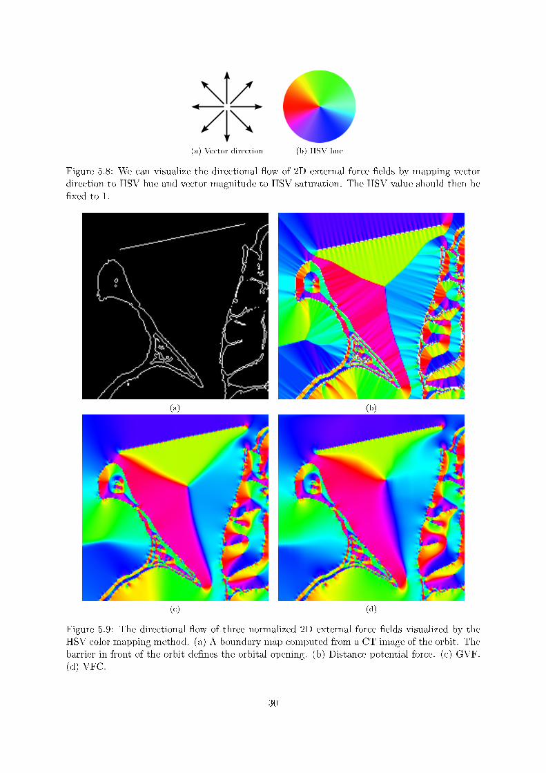
(a) Vector direction (b) HSV hue

Figure 5.8: We can visualize the directional �ow of 2D external force �elds by mapping vectordirection to HSV hue and vector magnitude to HSV saturation. The HSV value should then be�xed to 1.

(a) (b)

(c) (d)

Figure 5.9: The directional �ow of three normalized 2D external force �elds visualized by theHSV color mapping method. (a) A boundary map computed from a CT image of the orbit. Thebarrier in front of the orbit de�nes the orbital opening. (b) Distance potential force. (c) GVF.(d) VFC.

30

Chapter 6

Segmentation evaluation

Segmentation evaluation, i.e., the process of measuring and comparing the performance of dif-ferent segmentation methods in some particular application domain, is an essential step in thedevelopment of new segmentation methods for medical applications. A systematic framework forsegmentation evaluation was recently introduced by Udupa et al. [27]. This framework, whichis capable of handling both crisp and fuzzy segmentations, states that segmentation methodsshould be compared based on three factors: precision, accuracy, and e�ciency. We will coverthese factors in detail in the remaining sections of this chapter.

6.1 Precision

Segmentation precision is a measure of repeatability, i.e., how sensitive a segmentation methodis to operator input. The precision of a segmentation method M for a given situation Ti iscomputed as

PRMTi (O) =|CMO1

∩ CMO2|

|CMO1∪ CMO2

|,(6.1)

where CMO1and CMO2

are two fuzzy segmentations of an object O in some scene C. To assess theintra-operator precision of M , we let an operator segment the same object in the same scenetwice by using M . Similarly, to assess the inter-operator precision of M , we let two operatorssegment the same object in the same scene once by using M .

6.2 Accuracy

Segmentation accuracy denotes the degree to which a segmentation agrees with truth. Supposethat we want to assess the accuracy of a fuzzy segmentation CMO of some object O in a CTimage C. Because absolute true segmentation is generally not available for real CT images, the�rst thing we need to do is to choose an appropriate surrogate of true segmentation that wecan compare CMO with. We can obtain a fuzzy ground truth segmentation Ctd by, e.g., averagingmultiple manual segmentations performed by multiple experts [27]. Given Ctd, we assess theaccuracy of CMO by measuring two accuracy entities: sensitivity and speci�city. Sensitivity ismeasured as the true positive volume fraction

TPV FMd (O) =|CTP ||Ctd|

, (6.2)

31

C

C

C

C

C

C

C

TN

FN

FP

TP

td

OM

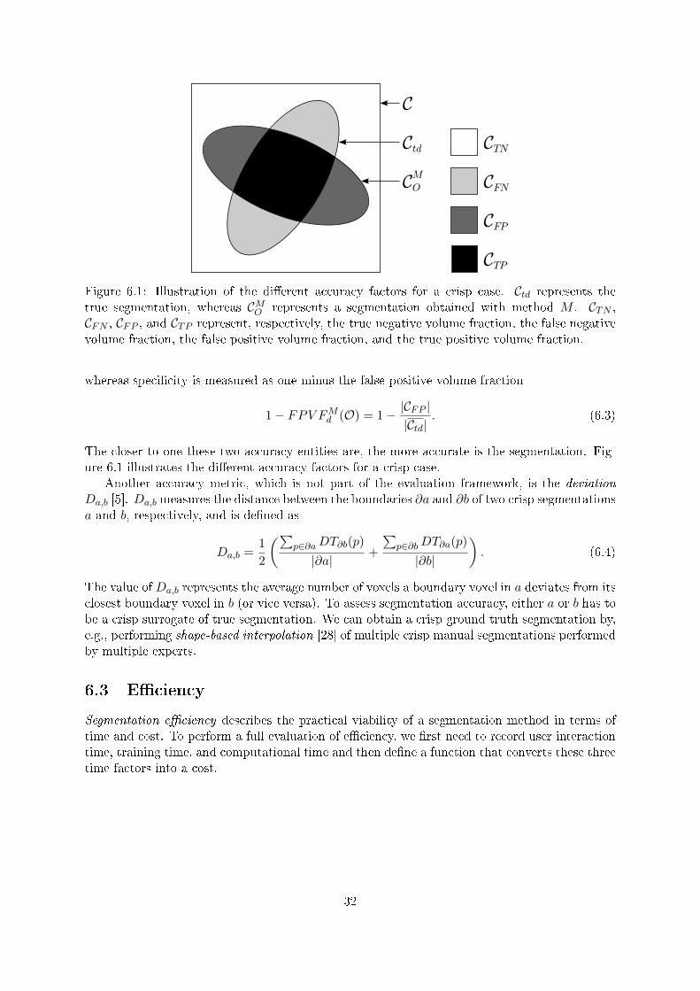
Figure 6.1: Illustration of the di�erent accuracy factors for a crisp case. Ctd represents thetrue segmentation, whereas CMO represents a segmentation obtained with method M . CTN ,CFN , CFP , and CTP represent, respectively, the true negative volume fraction, the false negativevolume fraction, the false positive volume fraction, and the true positive volume fraction.

whereas speci�city is measured as one minus the false positive volume fraction

1− FPV FMd (O) = 1− |CFP ||Ctd|

. (6.3)

The closer to one these two accuracy entities are, the more accurate is the segmentation. Fig-ure 6.1 illustrates the di�erent accuracy factors for a crisp case.

Another accuracy metric, which is not part of the evaluation framework, is the deviation

Da,b [5]. Da,b measures the distance between the boundaries ∂a and ∂b of two crisp segmentationsa and b, respectively, and is de�ned as

Da,b =1

2

(∑p∈∂aDT∂b(p)

|∂a|+

∑p∈∂bDT∂a(p)

|∂b|

). (6.4)

The value of Da,b represents the average number of voxels a boundary voxel in a deviates from itsclosest boundary voxel in b (or vice versa). To assess segmentation accuracy, either a or b has tobe a crisp surrogate of true segmentation. We can obtain a crisp ground truth segmentation by,e.g., performing shape-based interpolation [28] of multiple crisp manual segmentations performedby multiple experts.

6.3 E�ciency

Segmentation e�ciency describes the practical viability of a segmentation method in terms oftime and cost. To perform a full evaluation of e�ciency, we �rst need to record user interactiontime, training time, and computational time and then de�ne a function that converts these threetime factors into a cost.

32

Chapter 7

Volume visualization

Volume visualization is the process of exploring, transforming, and viewing volumetric dataas images. In this chapter, we review two commonly used volume visualization techniques:multi-planar reformatting (Section 7.1) and hardware-accelerated direct volume rendering (Sec-tion 7.2).

7.1 Multi-planar reformatting

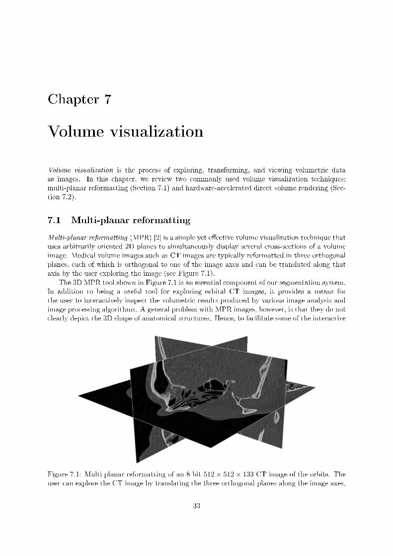
Multi-planar reformatting (MPR) [2] is a simple yet e�ective volume visualization technique thatuses arbitrarily oriented 2D planes to simultaneously display several cross-sections of a volumeimage. Medical volume images such as CT images are typically reformatted in three orthogonalplanes, each of which is orthogonal to one of the image axes and can be translated along thataxis by the user exploring the image (see Figure 7.1).

The 3D MPR tool shown in Figure 7.1 is an essential component of our segmentation system.In addition to being a useful tool for exploring orbital CT images, it provides a means forthe user to interactively inspect the volumetric results produced by various image analysis andimage processing algorithms. A general problem with MPR images, however, is that they do notclearly depict the 3D shape of anatomical structures. Hence, to facilitate some of the interactive

Figure 7.1: Multi-planar reformatting of an 8-bit 512× 512× 133 CT image of the orbits. Theuser can explore the CT image by translating the three orthogonal planes along the image axes.

33

steps in our proposed segmentation method (see Section 5.4), e.g., the positioning of landmarkson the orbital rim, we should supplement MPR with more sophisticated volume visualizationtechniques.

7.2 Hardware-accelerated direct volume rendering

Volume rendering is the process of creating 2D projections of 3D data [4]. In contrast to surfacerendering [4], volume rendering does not generate explicit geometric representations of imageobjects, but operates directly on the volumetric data, considering each voxel as a geometricprimitive with its own surface. The primary objective of volume rendering is typically not tocreate realistic images, but rather to create informative images from which human observers caneasily derive features of interest.

GPU-based ray-casting [29, 30] is an e�cient, �exible, and widely used volume renderingtechnique that exploits the intrinsic parallelism on modern GPUs. Suppose that we have avolumetric CT image that we want to project onto a planar display. The basic idea of ray-casting is to determine the values of the fragments (i.e., the pixel candidates) by casting aray from each fragment into the volume image. As the ray traverses the volume image, itgathers color and transparency information from the voxels it passes through. This informationis processed by a ray function, of which objective is to determine the �nal value of the fragment.We can represent a ray parametrically as

r(t) = r0 + dt, (7.1)

where r0 = (x0, y0, z0) is the starting point of the ray, and d = (a, b, c) is the normalized raydirection vector. To determine the ray starting points and direction vectors for all fragments,we render the front- and back-face of the volume's bounding box to 2D RGB textures, encodingtexture coordinates as RGB colors. The starting points of the rays are given by the front-facetexture. To obtain the direction vectors, we subtract the back-face texture from the front-facetexture and store the di�erence in a 2D RGBA texture; the length of each direction vector isstored in the texture's alpha channel and represents the maximum distance for the ray traversal.Given the ray starting points and direction vectors, we store the input volume image in a 3Dtexture and let the fragment shader of the GPU perform the ray-casting in a single, parallel passby sampling the 3D texture along the rays. For each ray r(t), the fragment shader initializes tto zero and then increments t with some pre-de�ned step length ∆t until r(t) hits the back-faceof the bounding box or is terminated early by the ray function. As a �nal step, the resultingimage is blended back to the display.

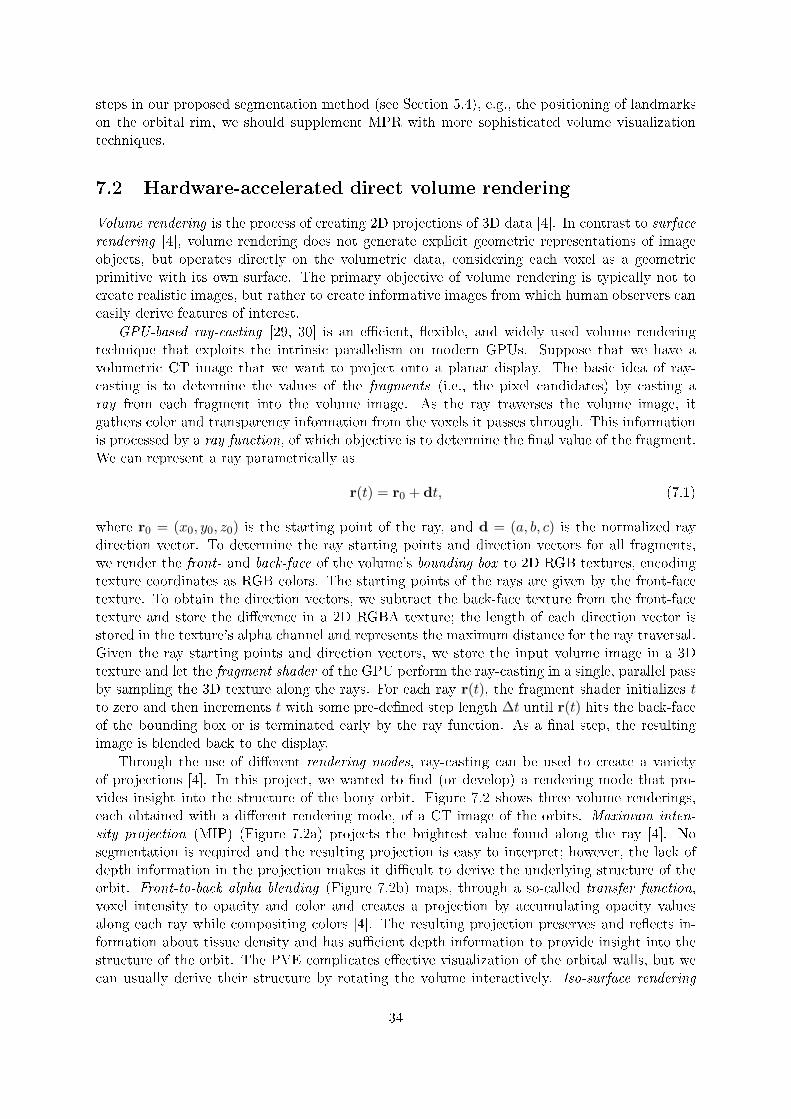
Through the use of di�erent rendering modes, ray-casting can be used to create a varietyof projections [4]. In this project, we wanted to �nd (or develop) a rendering mode that pro-vides insight into the structure of the bony orbit. Figure 7.2 shows three volume renderings,each obtained with a di�erent rendering mode, of a CT image of the orbits. Maximum inten-

sity projection (MIP) (Figure 7.2a) projects the brightest value found along the ray [4]. Nosegmentation is required and the resulting projection is easy to interpret; however, the lack ofdepth information in the projection makes it di�cult to derive the underlying structure of theorbit. Front-to-back alpha blending (Figure 7.2b) maps, through a so-called transfer function,voxel intensity to opacity and color and creates a projection by accumulating opacity valuesalong each ray while compositing colors [4]. The resulting projection preserves and re�ects in-formation about tissue density and has su�cient depth information to provide insight into thestructure of the orbit. The PVE complicates e�ective visualization of the orbital walls, but wecan usually derive their structure by rotating the volume interactively. Iso-surface rendering

34

(a)

(b) (c)

Figure 7.2: Hardware-accelerated direct volume renderings of an 8-bit 512×512×133 CT imageof the orbits. (a) MIP. (b) Front-to-back alpha blending. (c) Iso-surface rendering.

(Figure 7.2c) extracts the �rst sample found along the ray of which value satis�es a pre-de�nedthreshold criteria (i.e., a global threshold) and then uses the gradient of the CT image for shad-ing computations [4]. The resulting projection is a shaded and highly realistic image of thefacial skeleton. In general, a global threshold cannot completely separate bone from the rest ofthe CT image (see Section 5.1.1), so extracted iso-surfaces tend to either include noise and softtissue or exclude parts of the thin bones that form the orbital walls.

35

36

Chapter 8

Haptics

When we interact with real-life 3D objects, the sense of touch (haptics) is an essential additionto our visual perception. During the last two decades, the development of haptic devices andhaptic rendering algorithms has made it possible to create haptic interfaces in which the usercan feel, touch, and manipulate virtual 3D objects in a natural and intuitive way. It has beendemonstrated by Vidholm et al. [3] that such interfaces greatly facilitate interactive segmentationof objects in volume images.

In this chapter, we provide a brief description of the design and functionality of haptic devices(Section 8.1). We also review two state-of-the-art haptic rendering algorithms (Section 8.2).

8.1 Haptic devices

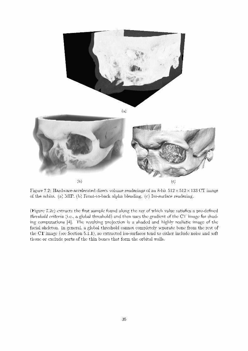
A haptic device is usually constructed as a small robot arm with a stylus or a ball that the userholds on to. Haptic feedback is given at the haptic probe, an interaction point located at the tipof the stylus or at the center of the ball. The number of independent translations or rotationsa haptic device can monitor and control (as input or output) are referred to as its degrees

of freedom (DOF). The feedback generated by a haptic device can be kinesthetic or tactile.

Figure 8.1: The PHANTOM Desktop haptic device from Sensable Technologies.

37

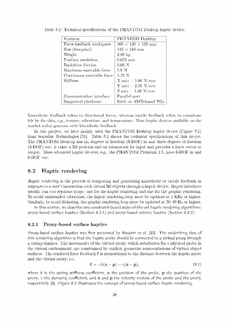
Table 8.1: Technical speci�cations of the PHANTOM Desktop haptic device.

Features PHANTOM Desktop

Force feedback workspace 160 × 120 × 120 mmSize (footprint) 143 × 184 mmWeight 2.86 kgPosition resolution 0.023 mmBackdrive friction 0.06 NMaximum exertable force 7.9 NContinuous exertable force 1.75 NSti�ness X axis > 1.86 N/mm

Y axis > 2.35 N/mmZ axis > 1.48 N/mm

Communication interface Parallel portSupported platforms Intel- or AMD-based PCs

Kinesthetic feedback refers to directional forces, whereas tactile feedback refers to sensationsfelt by the skin, e.g., texture, vibrations, and temperature. Most haptic devices available on themarket today generate only kinesthetic feedback.

In this project, we have mainly used the PHANTOM Desktop haptic device (Figure 8.1)from Sensable Technologies [31]. Table 8.1 shows the technical speci�cations of this device.The PHANTOM Desktop has six degrees of freedom (6-DOF) in and three degrees of freedom(3-DOF) out: it takes a 3D position and an orientation for input and provides a force vector asoutput. More advanced haptic devices, e.g., the PHANTOM Premium 1.5, have 6-DOF in and6-DOF out.

8.2 Haptic rendering

Haptic rendering is the process of computing and generating kinesthetic or tactile feedback inresponse to a user's interaction with virtual 3D objects through a haptic device. Haptic interfacesusually run two separate loops: one for the haptic rendering and one for the graphic rendering.To avoid unintended vibrations, the haptic rendering loop must be updates at 1 KHz or higher.Similarly, to avoid �ickering, the graphic rendering loop must be updated at 20�30 Hz or higher.

In this section, we describe two constraint-based state-of-the-art haptic rendering algorithms:proxy-based surface haptics (Section 8.2.1) and proxy-based volume haptics (Section 8.2.2).

8.2.1 Proxy-based surface haptics

Proxy-based surface haptics was �rst presented by Ruspini et al. [32]. The underlying idea ofthis rendering algorithm is that the haptic probe should be connected to a virtual proxy througha spring-damper. The movements of the virtual proxy, which substitutes for a physical probe inthe virtual environment, are constrained by explicit geometric representations of virtual objectsurfaces. The rendered force feedback f is proportional to the distance between the haptic probeand the virtual proxy, i.e.,

f = −k(x− p)− γ(x− p), (8.1)

where k is the spring sti�ness coe�cient, x the position of the probe, p the position of theproxy, γ the damping coe�cient, and x and p the velocity vectors of the probe and the proxy,respectively [3]. Figure 8.2 illustrates the concept of proxy-based surface haptic rendering.

38

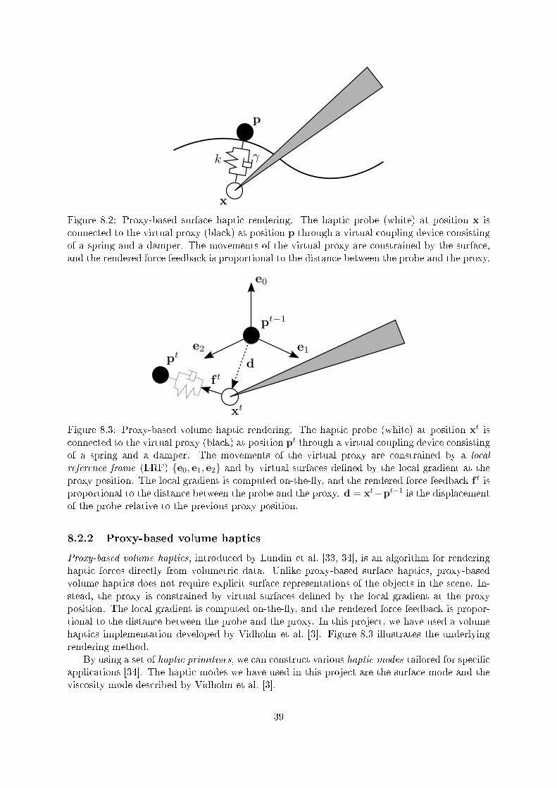
Figure 8.2: Proxy-based surface haptic rendering. The haptic probe (white) at position x isconnected to the virtual proxy (black) at position p through a virtual coupling device consistingof a spring and a damper. The movements of the virtual proxy are constrained by the surface,and the rendered force feedback is proportional to the distance between the probe and the proxy.

Figure 8.3: Proxy-based volume haptic rendering. The haptic probe (white) at position xt isconnected to the virtual proxy (black) at position pt through a virtual coupling device consistingof a spring and a damper. The movements of the virtual proxy are constrained by a local

reference frame (LRF) {e0, e1, e2} and by virtual surfaces de�ned by the local gradient at theproxy position. The local gradient is computed on-the-�y, and the rendered force feedback f t isproportional to the distance between the probe and the proxy. d = xt−pt−1 is the displacementof the probe relative to the previous proxy position.

8.2.2 Proxy-based volume haptics

Proxy-based volume haptics, introduced by Lundin et al. [33, 34], is an algorithm for renderinghaptic forces directly from volumetric data. Unlike proxy-based surface haptics, proxy-basedvolume haptics does not require explicit surface representations of the objects in the scene. In-stead, the proxy is constrained by virtual surfaces de�ned by the local gradient at the proxyposition. The local gradient is computed on-the-�y, and the rendered force feedback is propor-tional to the distance between the probe and the proxy. In this project, we have used a volumehaptics implementation developed by Vidholm et al. [3]. Figure 8.3 illustrates the underlyingrendering method.

By using a set of haptic primitives, we can construct various haptic modes tailored for speci�capplications [34]. The haptic modes we have used in this project are the surface mode and theviscosity mode described by Vidholm et al. [3].

39

40

Chapter 9

Development of a semi-automatic

system for orbit segmentation

In this chapter, we �rst discuss some related work on orbit segmentation (Section 9.1) andthen describe how we developed a prototype of a semi-automatic system for orbit segmentation(Section 9.2).

9.1 Related work

Many general-purpose systems for medical image analysis and visualization provide tools thatcan be used for manual segmentation of arbitrary objects in CT images. A few examples ofsuch systems are ITK-SNAP [35], OsiriX [36], and Mimics [37]. For each slice in the CTimage, the user utilizes a mouse or a stylus to outline or �ll regions corresponding to objectsof interest. Navigation between slices is typically performed with a keyboard. In order tocorrectly reconstruct 3D objects in CT images, the user must view and segment adjacent slicesin order. Regensburg et al. [38] found manual segmentation to be a reliable and accurate toolfor measuring orbital soft tissue volume, but did not assess its e�ciency.

Stratovan Maxillo [39] is a medical image segmentation system tailored for orbit segmenta-tion. It implements a semi-automatic segmentation method, in which the user �rst de�nes aset of anatomical landmarks and the system then automatically �ts a deformable surface modelto the orbit. The system provides advanced volume visualization tools and seems to produceaccurate orbit segmentations. A potential weakness of the system, however, is that the userinterface is designed for traditional 2D input devices. The semi-automatic segmentation processinvolves complex 3D interaction tasks that would probably be more natural and intuitive for ahuman user to carry out with a 6-DOF 3D input device.

Lamecker et al. [40, 41] developed a statistical 3D shape model (atlas) of the orbit, with theintention of using it for automatic segmentation and reconstruction of orbits in CT images. Inan initial case study, they demonstrated that the atlas was able to capture the shape variabilityof normal orbits. However, they found the generalization ability of the atlas to be insu�cientfor routine clinical usage. Fractured orbits display a high shape variability that is di�cult tocapture in an atlas, and the segmentation is further complicated by noise and PVE artifacts.

9.2 An orbit segmentation system based on the WISH toolkit

We developed our orbit segmentation system as an extension of an existing software toolkit forinteractive segmentation with haptics. This toolkit, WISH, was developed by Vidholm et al. [3, 5]

41

wishH3DGVFFilter

WISH

H3D API

WISHH3DOpenGL

OpenHaptics

Graphicswindow

C++

Python

TkInterGUI

X3D

Hapticdevice

Hapticdevice

wishH3DFuzzyConnectednessFilter

wishH3DDeformableSimplexMesh

wishH3DVolumeHaptics

wishH3DVolumeRenderer

wishH3DVolumeSlicer

wishH3DVolume

...

Figure 9.1: The software architecture of WISH and WISHH3D.

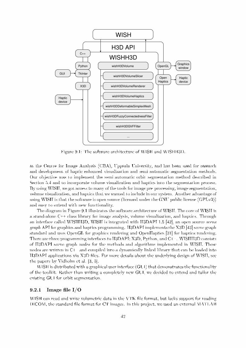
at the Centre for Image Analysis (CBA), Uppsala University, and has been used for researchand development of haptic-enhanced visualization and semi-automatic segmentation methods.Our objective was to implement the semi-automatic orbit segmentation method described inSection 5.4 and to incorporate volume visualization and haptics into the segmentation process.By using WISH, we got access to many of the tools for image pre-processing, image segmentation,volume visualization, and haptics that we wanted to include in our system. Another advantage ofusing WISH is that the software is open source (licensed under the GNU public license (GPLv3))and easy to extend with new functionality.

The diagram in Figure 9.1 illustrates the software architecture of WISH. The core of WISH isa stand-alone C++ class library for image analysis, volume visualization, and haptics. Throughan interface called WISHH3D, WISH is integrated with H3DAPI 1.5 [42], an open source scenegraph API for graphics and haptics programming. H3DAPI implements the X3D [43] scene graphstandard and uses OpenGL for graphics rendering and OpenHaptics [31] for haptics rendering.There are three programming interfaces to H3DAPI: X3D, Python, and C++. WISHH3D consistsof H3DAPI scene graph nodes for the methods and algorithms implemented in WISH. Thesenodes are written in C++ and compiled into a dynamically linked library that can be loaded intoH3DAPI applications via X3D �les. For more details about the underlying design of WISH, seethe papers by Vidholm et al. [3, 5].

WISH is distributed with a graphical user interface (GUI) that demonstrates the functionalityof the toolkit. Rather than writing a completely new GUI, we decided to extend and tailor theexisting GUI for orbit segmentation.

9.2.1 Image �le I/O

WISH can read and write volumetric data in the VTK �le format, but lacks support for readingDICOM, the standard �le format for CT images. In this project, we used an external MATLAB

42

script to convert DICOM CT images to VTK volumes. Future work includes extending WISHto handle DICOM images natively.

9.2.2 Image analysis and image processing tools

WISH contains several image analysis and image processing tools. We found the following toolsuseful to include in our orbit segmentation system:

• wishH3DBilateralFilter

• wishH3DCompareSegmentations

• wishH3DDeformableSimplexMesh

• wishH3DDistanceMapFilter

• wishH3DFuzzyConnectednessFilter (multi-seeded)• wishH3DGVFFilter

• wishH3DGaussianGradientsFilter

• wishH3DGaussianSmoothingFilter

• wishH3DThresholdFilter

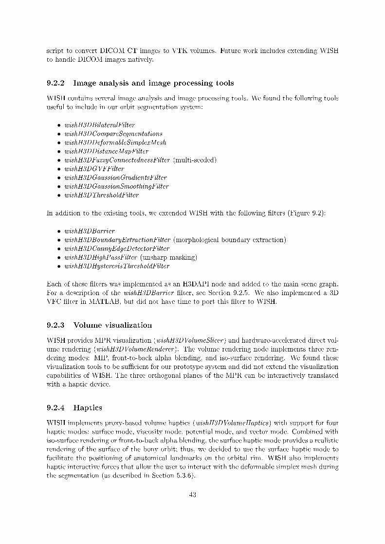
In addition to the existing tools, we extended WISH with the following �lters (Figure 9.2):

• wishH3DBarrier

• wishH3DBoundaryExtractionFilter (morphological boundary extraction)• wishH3DCannyEdgeDetectorFilter

• wishH3DHighPassFilter (unsharp masking)• wishH3DHysteresisThresholdFilter

Each of these �lters was implemented as an H3DAPI node and added to the main scene graph.For a description of the wishH3DBarrier �lter, see Section 9.2.5. We also implemented a 3DVFC �lter in MATLAB, but did not have time to port this �lter to WISH.

9.2.3 Volume visualization

WISH provides MPR visualization (wishH3DVolumeSlicer) and hardware-accelerated direct vol-ume rendering (wishH3DVolumeRenderer). The volume rendering node implements three ren-dering modes: MIP, front-to-back alpha blending, and iso-surface rendering. We found thesevisualization tools to be su�cient for our prototype system and did not extend the visualizationcapabilities of WISH. The three orthogonal planes of the MPR can be interactively translatedwith a haptic device.

9.2.4 Haptics

WISH implements proxy-based volume haptics (wishH3DVolumeHaptics) with support for fourhaptic modes: surface mode, viscosity mode, potential mode, and vector mode. Combined withiso-surface rendering or front-to-back alpha blending, the surface haptic mode provides a realisticrendering of the surface of the bony orbit; thus, we decided to use the surface haptic mode tofacilitate the positioning of anatomical landmarks on the orbital rim. WISH also implementshaptic interactive forces that allow the user to interact with the deformable simplex mesh duringthe segmentation (as described in Section 5.3.6).

43

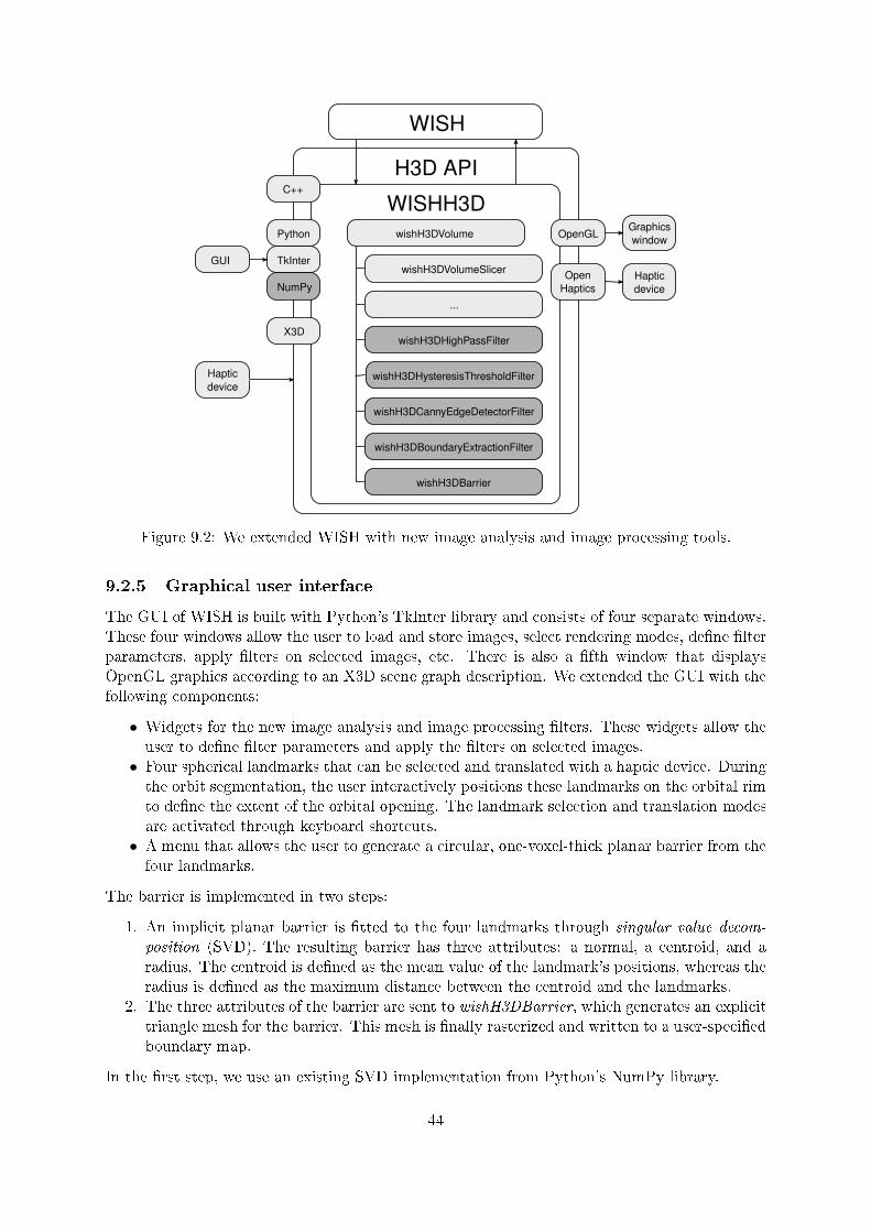
WISH

H3D API

WISHH3DOpenGL

OpenHaptics

Graphicswindow

C++

Python

TkInterGUI

X3D

Hapticdevice

Hapticdevice

wishH3DVolumeSlicer

wishH3DVolume

NumPy

wishH3DHighPassFilter

wishH3DBarrier

wishH3DBoundaryExtractionFilter

wishH3DHysteresisThresholdFilter

wishH3DCannyEdgeDetectorFilter

...

Figure 9.2: We extended WISH with new image analysis and image processing tools.

9.2.5 Graphical user interface

The GUI of WISH is built with Python's TkInter library and consists of four separate windows.These four windows allow the user to load and store images, select rendering modes, de�ne �lterparameters, apply �lters on selected images, etc. There is also a �fth window that displaysOpenGL graphics according to an X3D scene graph description. We extended the GUI with thefollowing components:

• Widgets for the new image analysis and image processing �lters. These widgets allow theuser to de�ne �lter parameters and apply the �lters on selected images.• Four spherical landmarks that can be selected and translated with a haptic device. Duringthe orbit segmentation, the user interactively positions these landmarks on the orbital rimto de�ne the extent of the orbital opening. The landmark selection and translation modesare activated through keyboard shortcuts.• A menu that allows the user to generate a circular, one-voxel-thick planar barrier from thefour landmarks.

The barrier is implemented in two steps:

1. An implicit planar barrier is �tted to the four landmarks through singular value decom-

position (SVD). The resulting barrier has three attributes: a normal, a centroid, and aradius. The centroid is de�ned as the mean value of the landmark's positions, whereas theradius is de�ned as the maximum distance between the centroid and the landmarks.

2. The three attributes of the barrier are sent to wishH3DBarrier, which generates an explicittriangle mesh for the barrier. This mesh is �nally rasterized and written to a user-speci�edboundary map.

In the �rst step, we use an existing SVD implementation from Python's NumPy library.

44

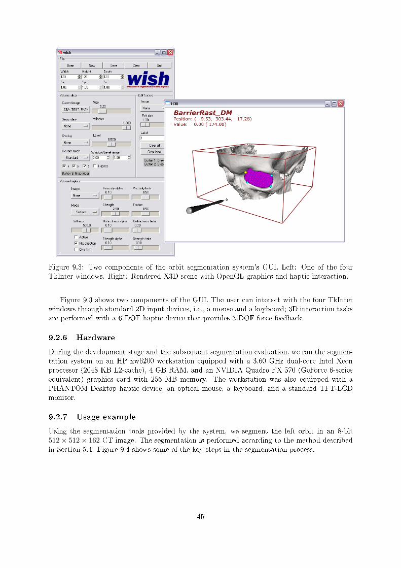
Figure 9.3: Two components of the orbit segmentation system's GUI. Left: One of the fourTkInter windows. Right: Rendered X3D scene with OpenGL graphics and haptic interaction.

Figure 9.3 shows two components of the GUI. The user can interact with the four TkInterwindows through standard 2D input devices, i.e., a mouse and a keyboard; 3D interaction tasksare performed with a 6-DOF haptic device that provides 3-DOF force feedback.

9.2.6 Hardware

During the development stage and the subsequent segmentation evaluation, we ran the segmen-tation system on an HP xw6200 workstation equipped with a 3.60 GHz dual-core Intel Xeonprocessor (2048 KB L2-cache), 4 GB RAM, and an NVIDIA Quadro FX 570 (GeForce 6-seriesequivalent) graphics card with 256 MB memory. The workstation was also equipped with aPHANTOM Desktop haptic device, an optical mouse, a keyboard, and a standard TFT-LCDmonitor.

9.2.7 Usage example

Using the segmentation tools provided by the system, we segment the left orbit in an 8-bit512× 512× 162 CT image. The segmentation is performed according to the method describedin Section 5.4. Figure 9.4 shows some of the key steps in the segmentation process.

45

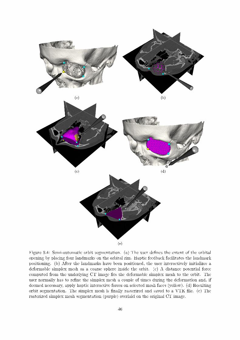
(a) (b)

(c) (d)

(e)

Figure 9.4: Semi-automatic orbit segmentation. (a) The user de�nes the extent of the orbitalopening by placing four landmarks on the orbital rim. Haptic feedback facilitates the landmarkpositioning. (b) After the landmarks have been positioned, the user interactively initializes adeformable simplex mesh as a coarse sphere inside the orbit. (c) A distance potential forcecomputed from the underlying CT image �ts the deformable simplex mesh to the orbit. Theuser normally has to re�ne the simplex mesh a couple of times during the deformation and, ifdeemed necessary, apply haptic interactive forces on selected mesh faces (yellow). (d) Resultingorbit segmentation. The simplex mesh is �nally rasterized and saved to a VTK �le. (e) Therasterized simplex mesh segmentation (purple) overlaid on the original CT image.

46

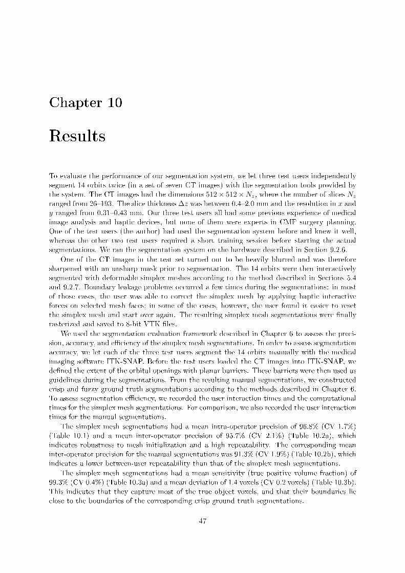
Chapter 10

Results

To evaluate the performance of our segmentation system, we let three test users independentlysegment 14 orbits twice (in a set of seven CT images) with the segmentation tools provided bythe system. The CT images had the dimensions 512× 512×Nz, where the number of slices Nz

ranged from 26�193. The slice thickness ∆z was between 0.4�2.0 mm and the resolution in x andy ranged from 0.31�0.43 mm. Our three test users all had some previous experience of medicalimage analysis and haptic devices, but none of them were experts in CMF surgery planning.One of the test users (the author) had used the segmentation system before and knew it well,whereas the other two test users required a short training session before starting the actualsegmentations. We ran the segmentation system on the hardware described in Section 9.2.6.

One of the CT images in the test set turned out to be heavily blurred and was thereforesharpened with an unsharp mask prior to segmentation. The 14 orbits were then interactivelysegmented with deformable simplex meshes according to the method described in Sections 5.4and 9.2.7. Boundary leakage problems occurred a few times during the segmentations: in mostof those cases, the user was able to correct the simplex mesh by applying haptic interactiveforces on selected mesh faces; in some of the cases, however, the user found it easier to resetthe simplex mesh and start over again. The resulting simplex mesh segmentations were �nallyrasterized and saved to 8-bit VTK �les.

We used the segmentation evaluation framework described in Chapter 6 to assess the preci-sion, accuracy, and e�ciency of the simplex mesh segmentations. In order to assess segmentationaccuracy, we let each of the three test users segment the 14 orbits manually with the medicalimaging software ITK-SNAP. Before the test users loaded the CT images into ITK-SNAP, wede�ned the extent of the orbital openings with planar barriers. These barriers were then used asguidelines during the segmentations. From the resulting manual segmentations, we constructedcrisp and fuzzy ground truth segmentations according to the methods described in Chapter 6.To assess segmentation e�ciency, we recorded the user interaction times and the computationaltimes for the simplex mesh segmentations. For comparison, we also recorded the user interactiontimes for the manual segmentations.

The simplex mesh segmentations had a mean intra-operator precision of 96.8% (CV 1.7%)(Table 10.1) and a mean inter-operator precision of 95.7% (CV 2.1%) (Table 10.2a), whichindicates robustness to mesh initialization and a high repeatability. The corresponding meaninter-operator precision for the manual segmentations was 91.3% (CV 1.9%) (Table 10.2b), whichindicates a lower between-user repeatability than that of the simplex mesh segmentations.

The simplex mesh segmentations had a mean sensitivity (true positive volume fraction) of99.3% (CV 0.4%) (Table 10.3a) and a mean deviation of 1.4 voxels (CV 0.2 voxels) (Table 10.3b).This indicates that they capture most of the true object voxels, and that their boundaries lieclose to the boundaries of the corresponding crisp ground truth segmentations.

47

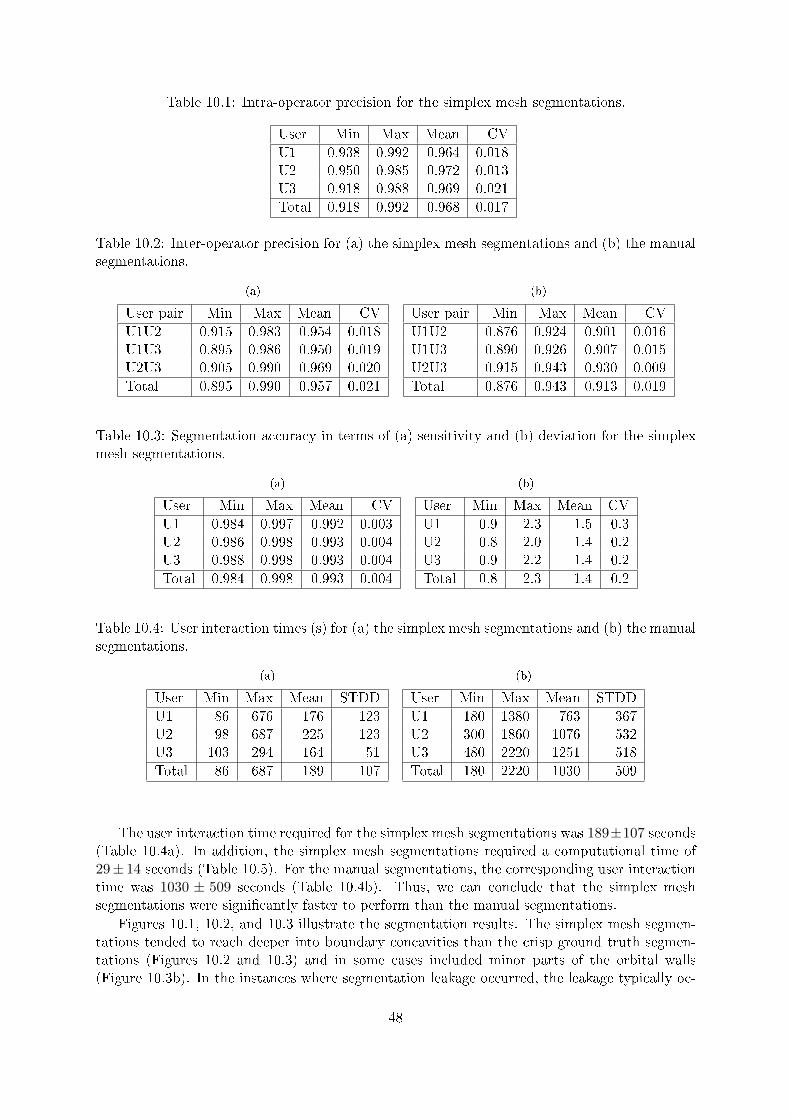
Table 10.1: Intra-operator precision for the simplex mesh segmentations.

User Min Max Mean CV

U1 0.938 0.992 0.964 0.018U2 0.950 0.985 0.972 0.013U3 0.918 0.988 0.969 0.021

Total 0.918 0.992 0.968 0.017

Table 10.2: Inter-operator precision for (a) the simplex mesh segmentations and (b) the manualsegmentations.

(a)

User pair Min Max Mean CV

U1U2 0.915 0.983 0.954 0.018U1U3 0.895 0.986 0.950 0.019U2U3 0.905 0.990 0.969 0.020

Total 0.895 0.990 0.957 0.021

(b)

User pair Min Max Mean CV

U1U2 0.876 0.924 0.901 0.016U1U3 0.890 0.926 0.907 0.015U2U3 0.915 0.943 0.930 0.009

Total 0.876 0.943 0.913 0.019

Table 10.3: Segmentation accuracy in terms of (a) sensitivity and (b) deviation for the simplexmesh segmentations.

(a)

User Min Max Mean CV

U1 0.984 0.997 0.992 0.003U2 0.986 0.998 0.993 0.004U3 0.988 0.998 0.993 0.004

Total 0.984 0.998 0.993 0.004

(b)

User Min Max Mean CV

U1 0.9 2.3 1.5 0.3U2 0.8 2.0 1.4 0.2U3 0.9 2.2 1.4 0.2

Total 0.8 2.3 1.4 0.2

Table 10.4: User interaction times (s) for (a) the simplex mesh segmentations and (b) the manualsegmentations.

(a)

User Min Max Mean STDD

U1 86 676 176 123U2 98 687 225 123U3 103 294 164 51

Total 86 687 189 107

(b)

User Min Max Mean STDD

U1 180 1380 763 367U2 300 1860 1076 532U3 480 2220 1251 518

Total 180 2220 1030 509

The user interaction time required for the simplex mesh segmentations was 189±107 seconds(Table 10.4a). In addition, the simplex mesh segmentations required a computational time of29± 14 seconds (Table 10.5). For the manual segmentations, the corresponding user interactiontime was 1030 ± 509 seconds (Table 10.4b). Thus, we can conclude that the simplex meshsegmentations were signi�cantly faster to perform than the manual segmentations.

Figures 10.1, 10.2, and 10.3 illustrate the segmentation results. The simplex mesh segmen-tations tended to reach deeper into boundary concavities than the crisp ground truth segmen-tations (Figures 10.2 and 10.3) and in some cases included minor parts of the orbital walls(Figure 10.3b). In the instances where segmentation leakage occurred, the leakage typically oc-

48

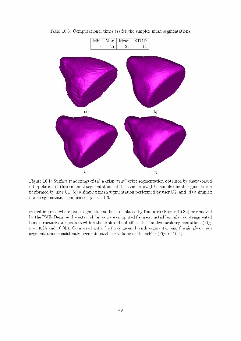
Table 10.5: Computational times (s) for the simplex mesh segmentations.

Min Max Mean STDD

6 45 29 14

(a) (b)

(c) (d)

Figure 10.1: Surface renderings of (a) a crisp �true� orbit segmentation obtained by shape-basedinterpolation of three manual segmentations of the same orbit, (b) a simplex mesh segmentationperformed by user U1, (c) a simplex mesh segmentation performed by user U2, and (d) a simplexmesh segmentation performed by user U3.

curred in areas where bone segments had been displaced by fractures (Figure 10.3b) or removedby the PVE. Because the external forces were computed from extracted boundaries of segmentedbone structures, air pockets within the orbit did not a�ect the simplex mesh segmentations (Fig-ure 10.2b and 10.3b). Compared with the fuzzy ground truth segmentations, the simplex meshsegmentations consistently overestimated the volume of the orbits (Figure 10.4).

49

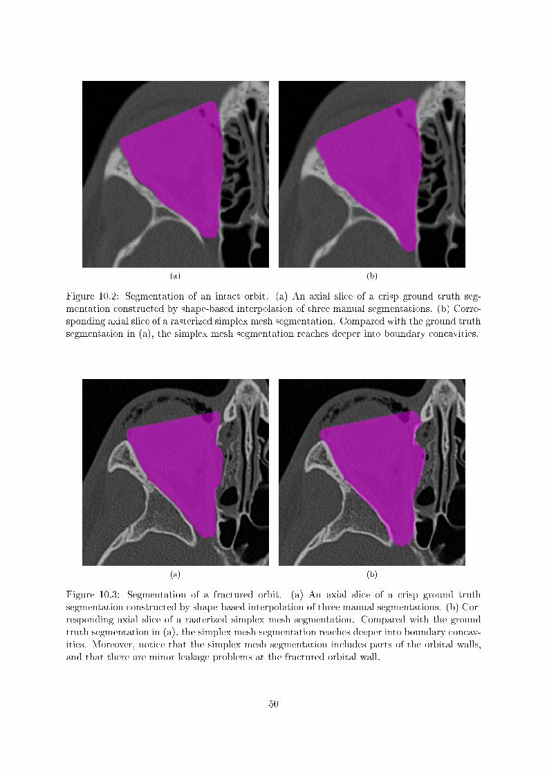
(a) (b)

Figure 10.2: Segmentation of an intact orbit. (a) An axial slice of a crisp ground truth seg-mentation constructed by shape-based interpolation of three manual segmentations. (b) Corre-sponding axial slice of a rasterized simplex mesh segmentation. Compared with the ground truthsegmentation in (a), the simplex mesh segmentation reaches deeper into boundary concavities.

(a) (b)

Figure 10.3: Segmentation of a fractured orbit. (a) An axial slice of a crisp ground truthsegmentation constructed by shape-based interpolation of three manual segmentations. (b) Cor-responding axial slice of a rasterized simplex mesh segmentation. Compared with the groundtruth segmentation in (a), the simplex mesh segmentation reaches deeper into boundary concav-ities. Moreover, notice that the simplex mesh segmentation includes parts of the orbital walls,and that there are minor leakage problems at the fractured orbital wall.

50

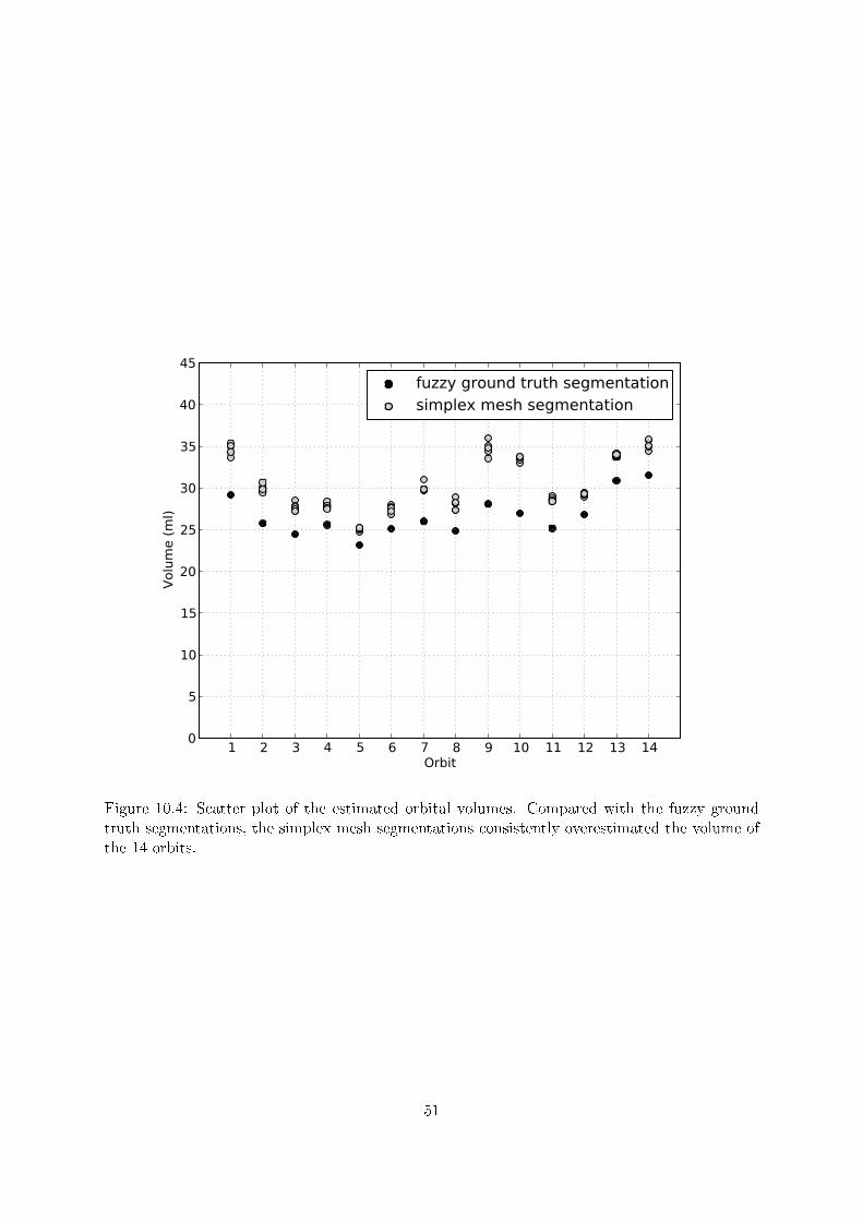
1 2 3 4 5 6 7 8 9 10 11 12 13 14Orbit

0

5

10

15

20

25

30

35

40

45

Volu

me

(ml)

fuzzy ground truth segmentationsimplex mesh segmentation

Figure 10.4: Scatter plot of the estimated orbital volumes. Compared with the fuzzy groundtruth segmentations, the simplex mesh segmentations consistently overestimated the volume ofthe 14 orbits.

51

52

Chapter 11

Summary and conclusions

In this chapter, we summarize and conclude this master's thesis project. We also provide somesuggestions for future work.

11.1 Summary

In this master's thesis project, we developed a prototype of a semi-automatic system for seg-menting orbits in CT images. The underlying segmentation method consists of three mainstages. In the �rst stage, we use hysteresis thresholding and morphological boundary extractionto segment and extract the boundaries of the bone structures in the orbit. In the second stage,we de�ne the extent of the orbital opening by placing four landmarks on the orbital rim. Tothese landmarks, we �t a planar barrier that we rasterize and write to the boundary map. Inthe third and �nal stage, we compute a distance potential force from the boundary map and usethe resulting force to �t an interactive deformable simplex mesh to the orbit.

We developed the segmentation system as an extension of WISH, an existing open sourcesoftware toolkit for interactive segmentation with haptic interaction. A GUI with volume visu-alization tools and haptic feedback allows the user to explore the underlying CT image, de�neanatomical landmarks, and guide the deformable simplex mesh through the segmentation.

To evaluate the performance of our segmentation system, we let three test users indepen-dently segment 14 orbits twice (in a set of seven CT images) with the segmentation tools providedby the system. In order to assess segmentation accuracy, we constructed crisp and fuzzy groundtruth segmentations from manual orbit segmentations performed by the three test users. Theresults of this case study indicate that our segmentation system can be used to obtain fast andaccurate orbit segmentations, with high intra-operator and inter-operator precision.

For information about the availability of the source code for the segmentation system, pleasevisit the project's web page1.

11.2 Conclusions

Separating bone and soft tissue in orbital CT images is a non-trivial task due to the presence ofnoise and PVE artifacts. To obtain accurate segmentations of the thin bone structures in the or-bit, we have to employ segmentation methods that not only consider the intensities of the voxelsbut also their spatial relationships. We showed that both the hysteresis thresholding method andthe multi-seeded fuzzy connectedness segmentation method are capable of producing su�ciently

1http://www.cb.uu.se/research/haptics/orbitproject

53

accurate segmentation results. An advantage of using the multi-seeded fuzzy connectedness ap-proach over hysteresis thresholding is that we do not have to identify a lower threshold tl for bonetissue; moreover, by providing a fuzzy object representation, multi-seeded fuzzy connectednesssegmentation preserves more information about the segmented bone structures. However, theseadvantages come at the expense of a higher computational complexity.

The deformable simplex mesh used in the segmentation system can represent objects ofwidely di�erent shapes and is also robust to noise and boundary gaps. These desirable propertiesmake it a suitable tool for segmenting intact as well as injured orbits in CT images corruptedby noise and PVE artifacts. We demonstrated that the distance potential force was able toaccurately �t the deformable simplex mesh to the 14 orbits in the test set, although some ofthe segmentations required interactive correction. Replacing the distance potential force witha GVF or VFC �eld would probably improve the robustness and accuracy of our segmentationmethod, but also increase its computational cost.

As expected, the manual orbit segmentations turned out to be tedious and time-consumingto perform. We observed an average interaction time of 17 minutes. The simplex mesh segmen-tations required signi�cantly less interaction time�only three minutes on average. They alsohad a higher intra-operator precision than the manual segmentations. These results con�rmsome of the expected bene�ts of semi-automatic segmentation over manual segmentation.

Compared with the crisp and fuzzy ground truth segmentations we constructed from themanual segmentations, the simplex mesh segmentations reached deeper into boundary concavi-ties and thereby overestimated the volume of the orbits. Some of the simplex mesh segmentationsalso included minor parts of the orbital walls. It should be emphasized, however, that none ofthe test users who performed the manual segmentations were experts in CMF surgery planning;thus, it is uncertain whether the ground truth segmentations are more correct than the simplexmesh segmentations.

During the case study, we noticed that the two untrained test users were able to use thesegmentation system more or less independently after a short training session. Although theyinitially required considerably more time than the experienced test user to segment the orbits,their mean user interaction times were similar to that of the experienced test user. These resultsindicate that the segmentation system is fairly simple and intuitive to use.

Furthermore, we found that haptic interaction, via a haptic-enabled 6-DOF input device,facilitated the positioning of anatomical landmarks and allowed the test users to interact with thedeformable simplex mesh in a natural and intuitive way. The haptic interactive forces providedan e�ective means for the test users to correct defects in the simplex mesh segmentations. Ourcase study supports the statement that haptic feedback and 3D interaction facilitate interactivesegmentation of volume images; however, it does not establish whether haptic feedback actuallyimproves the performance of our segmentation method.

In conclusion, we have demonstrated that it is possible to obtain fast and accurate orbitsegmentations by combining semi-automatic segmentation tools with volume visualization andhaptics. Although the current segmentation system is a prototype, it has the potential to beused in routine clinical practice after further improvement and testing.

11.3 Future work

To con�rm the accuracy of our proposed segmentation method, both the simplex mesh seg-mentations and the ground truth segmentations should be visually inspected by an expert inCMF surgery planning. Future work should also include evaluation of segmentation speci�city.Because speci�city depends on the size of the scene domain, such an evaluation would requirethe segmented CT volumes to be cropped around the orbits in a consistent way.

54

In order to determine whether haptic feedback improves segmentation accuracy, precision,or e�ciency, we need to perform the simplex mesh segmentations with and without hapticfeedback. It would also be interesting to investigate whether stereo graphics or head trackingcan be used to facilitate the segmentation. Preliminary tests we conducted with anaglyph stereographics indicate that binocular depth cues signi�cantly facilitate the positioning of anatomicallandmarks on the orbital rim.

The planar barriers we generated from the four user-de�ned landmarks did not follow thenatural curvature of the orbital rims. Future work should evaluate whether these deviations a�ectthe segmentation accuracy. The outcome of such an evaluation should then decide whether thereis a need for developing more sophisticated methods for de�ning the orbital opening. Since thereis no consensus about how to de�ne the extent of the orbital opening [38], these tasks wouldrequire close collaboration with expert physicians.

A limitation of the current segmentation system is that it only runs on 32-bit architectures.The 32-bit address space becomes a bottleneck when computing, e.g., Gaussian gradients orGVF �elds for large CT volumes. Hence, the segmentation system should be ported to a 64-bitarchitecture and operating system, in order to take advantage of the larger physical and virtualaddress spaces as well as the higher precision �xed-point math capabilities.

To improve the usability and e�ciency of the segmentation system, we should hide redun-dant GUI widgets and de�ne suitable parameter presets; moreover, we should streamline thecomputations of boundary maps and external forces.

Furthermore, the segmentation system lacks a tool for cropping the CT volume aroundthe orbits. Such a tool would allow us to reduce the amount of data and thereby speed upthe computations. The performance of the ray-caster can be improved by, e.g., implementinghierarchical data structures and empty space skipping [30]. Another, perhaps obvious way toimprove the rendering performance is to use a faster GPU with larger graphics memory.

Finally, we think it would be interesting to investigate whether the segmentation systemcan be used to segment other bone cavities in the cranium, e.g., the sinuses or the intra-cranialcavity.

55

56

Acknowledgments

I would like to acknowledge and thank the following people for their help and contributions to thismaster's thesis project. Special thanks to my supervisors, Ingela Nyström and Filip Malmberg,who gave me the opportunity to work on this project and provided valuable feedback and supportduring the work.

• Ingela Nyström1

• Filip Malmberg1

• Ewert Bengtsson1

• Fredrik Nysjö1

• Jan-Michaél Hirsch2

• Elias Messo2

• Roman Khonsari3

The project was supported by a grant from NovaMedTech4.

1Centre for Image Analysis (CBA), Uppsala University, Sweden2Department of Surgical Sciences, Oral & Maxillofacial Surgery, Uppsala University, Sweden3Department of Craniofacial Development, King's College, London4http://www.novamedtech.se

57

58

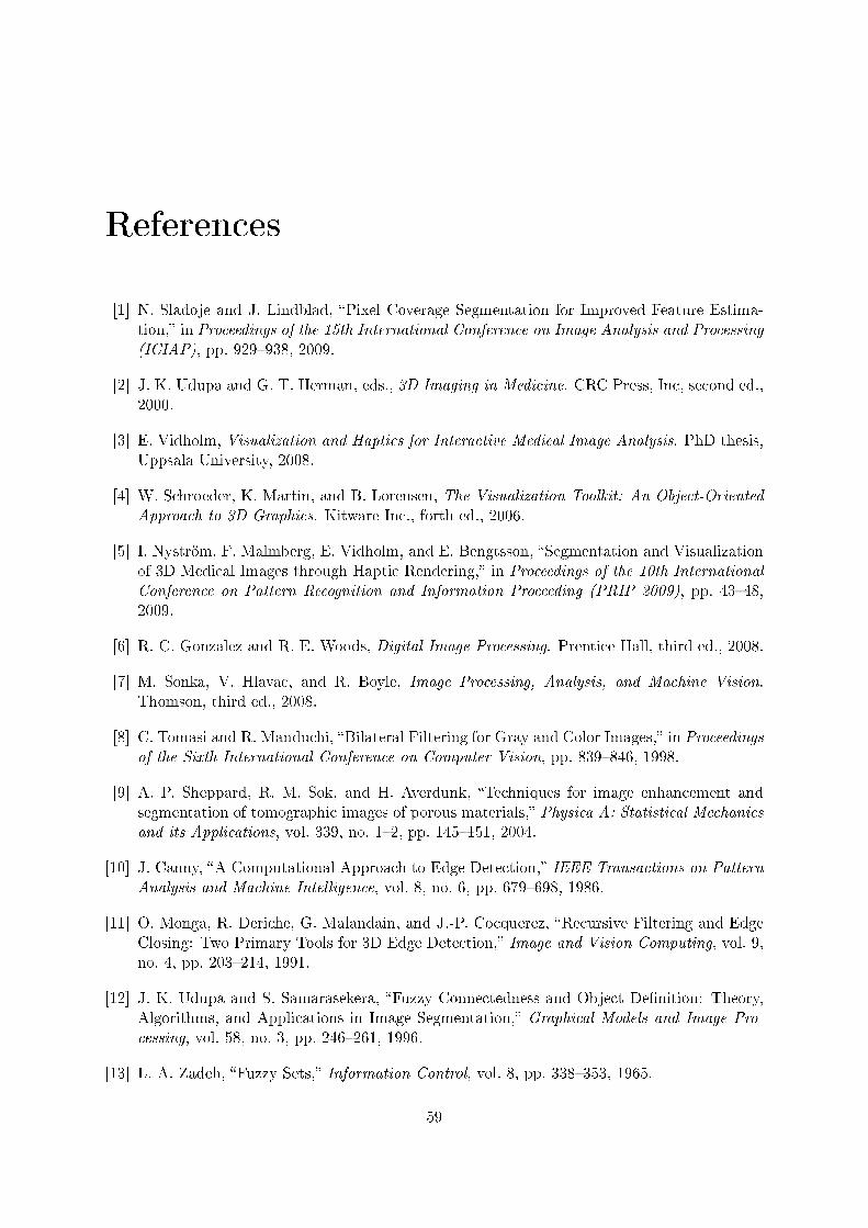
References

[1] N. Sladoje and J. Lindblad, �Pixel Coverage Segmentation for Improved Feature Estima-tion,� in Proceedings of the 15th International Conference on Image Analysis and Processing

(ICIAP), pp. 929�938, 2009.

[2] J. K. Udupa and G. T. Herman, eds., 3D Imaging in Medicine. CRC Press, Inc, second ed.,2000.

[3] E. Vidholm, Visualization and Haptics for Interactive Medical Image Analysis. PhD thesis,Uppsala University, 2008.

[4] W. Schroeder, K. Martin, and B. Lorensen, The Visualization Toolkit: An Object-Oriented

Approach to 3D Graphics. Kitware Inc., forth ed., 2006.

[5] I. Nyström, F. Malmberg, E. Vidholm, and E. Bengtsson, �Segmentation and Visualizationof 3D Medical Images through Haptic Rendering,� in Proceedings of the 10th International

Conference on Pattern Recognition and Information Proceeding (PRIP 2009), pp. 43�48,2009.

[6] R. C. Gonzalez and R. E. Woods, Digital Image Processing. Prentice Hall, third ed., 2008.

[7] M. Sonka, V. Hlavac, and R. Boyle, Image Processing, Analysis, and Machine Vision.Thomson, third ed., 2008.

[8] C. Tomasi and R. Manduchi, �Bilateral Filtering for Gray and Color Images,� in Proceedingsof the Sixth International Conference on Computer Vision, pp. 839�846, 1998.

[9] A. P. Sheppard, R. M. Sok, and H. Averdunk, �Techniques for image enhancement andsegmentation of tomographic images of porous materials,� Physica A: Statistical Mechanics

and its Applications, vol. 339, no. 1�2, pp. 145�151, 2004.

[10] J. Canny, �A Computational Approach to Edge Detection,� IEEE Transactions on Pattern

Analysis and Machine Intelligence, vol. 8, no. 6, pp. 679�698, 1986.

[11] O. Monga, R. Deriche, G. Malandain, and J.-P. Cocquerez, �Recursive Filtering and EdgeClosing: Two Primary Tools for 3D Edge Detection,� Image and Vision Computing, vol. 9,no. 4, pp. 203�214, 1991.

[12] J. K. Udupa and S. Samarasekera, �Fuzzy Connectedness and Object De�nition: Theory,Algorithms, and Applications in Image Segmentation,� Graphical Models and Image Pro-

cessing, vol. 58, no. 3, pp. 246�261, 1996.

[13] L. A. Zadeh, �Fuzzy Sets,� Information Control, vol. 8, pp. 338�353, 1965.

59

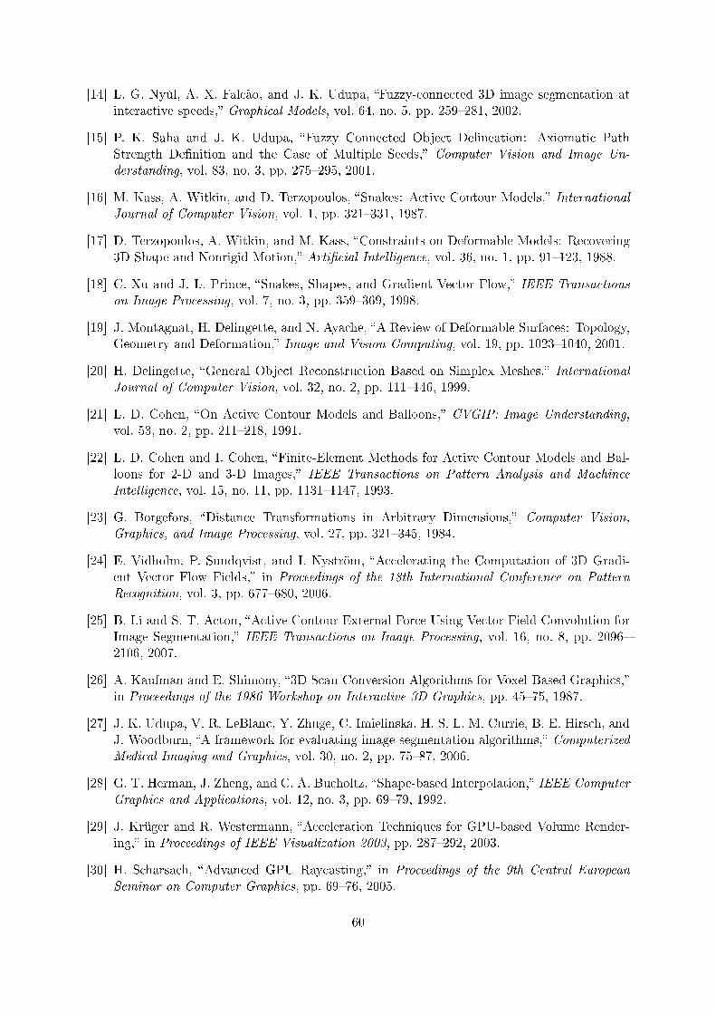
[14] L. G. Nyúl, A. X. Falcão, and J. K. Udupa, �Fuzzy-connected 3D image segmentation atinteractive speeds,� Graphical Models, vol. 64, no. 5, pp. 259�281, 2002.

[15] P. K. Saha and J. K. Udupa, �Fuzzy Connected Object Delineation: Axiomatic PathStrength De�nition and the Case of Multiple Seeds,� Computer Vision and Image Un-

derstanding, vol. 83, no. 3, pp. 275�295, 2001.

[16] M. Kass, A. Witkin, and D. Terzopoulos, �Snakes: Active Contour Models,� InternationalJournal of Computer Vision, vol. 1, pp. 321�331, 1987.

[17] D. Terzopoulos, A. Witkin, and M. Kass, �Constraints on Deformable Models: Recovering3D Shape and Nonrigid Motion,� Arti�cial Intelligence, vol. 36, no. 1, pp. 91�123, 1988.

[18] C. Xu and J. L. Prince, �Snakes, Shapes, and Gradient Vector Flow,� IEEE Transactions

on Image Processing, vol. 7, no. 3, pp. 359�369, 1998.

[19] J. Montagnat, H. Delingette, and N. Ayache, �A Review of Deformable Surfaces: Topology,Geometry and Deformation,� Image and Vision Computing, vol. 19, pp. 1023�1040, 2001.

[20] H. Delingette, �General Object Reconstruction Based on Simplex Meshes,� International

Journal of Computer Vision, vol. 32, no. 2, pp. 111�146, 1999.

[21] L. D. Cohen, �On Active Contour Models and Balloons,� CVGIP: Image Understanding,vol. 53, no. 2, pp. 211�218, 1991.

[22] L. D. Cohen and I. Cohen, �Finite-Element Methods for Active Contour Models and Bal-loons for 2-D and 3-D Images,� IEEE Transactions on Pattern Analysis and Machince

Intelligence, vol. 15, no. 11, pp. 1131�1147, 1993.

[23] G. Borgefors, �Distance Transformations in Arbitrary Dimensions,� Computer Vision,

Graphics, and Image Processing, vol. 27, pp. 321�345, 1984.

[24] E. Vidholm, P. Sundqvist, and I. Nyström, �Accelerating the Computation of 3D Gradi-ent Vector Flow Fields,� in Proceedings of the 18th International Conference on Pattern

Recognition, vol. 3, pp. 677�680, 2006.

[25] B. Li and S. T. Acton, �Active Contour External Force Using Vector Field Convolution forImage Segmentation,� IEEE Transactions on Image Processing, vol. 16, no. 8, pp. 2096�2106, 2007.

[26] A. Kaufman and E. Shimony, �3D Scan-Conversion Algorithms for Voxel-Based Graphics,�in Proceedings of the 1986 Workshop on Interactive 3D Graphics, pp. 45�75, 1987.

[27] J. K. Udupa, V. R. LeBlanc, Y. Zhuge, C. Imielinska, H. S. L. M. Currie, B. E. Hirsch, andJ. Woodburn, �A framework for evaluating image segmentation algorithms,� ComputerizedMedical Imaging and Graphics, vol. 30, no. 2, pp. 75�87, 2006.

[28] G. T. Herman, J. Zheng, and C. A. Bucholtz, �Shape-based Interpolation,� IEEE Computer

Graphics and Applications, vol. 12, no. 3, pp. 69�79, 1992.

[29] J. Krüger and R. Westermann, �Acceleration Techniques for GPU-based Volume Render-ing,� in Proceedings of IEEE Visualization 2003, pp. 287�292, 2003.

[30] H. Scharsach, �Advanced GPU Raycasting,� in Proceedings of the 9th Central European

Seminar on Computer Graphics, pp. 69�76, 2005.

60

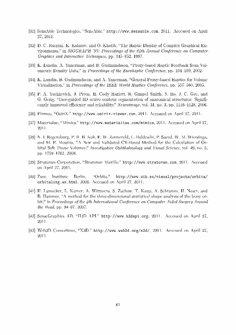
[31] SensAble Technologies, �SensAble.� http://www.sensable.com, 2011. Accessed on April27, 2011.

[32] D. C. Ruspini, K. Kolarov, and O. Khatib, �The Haptic Display of Complex Graphical En-vironments,� in SIGGRAPH '97: Proceedings of the 24th Annual Conference on Computer

Graphics and Interactive Techniques, pp. 345�352, 1997.

[33] K. Lundin, A. Ynnerman, and B. Gudmundsson, �Proxy-based Haptic Feedback from Vol-umetric Density Data,� in Proceedings of the Eurohaptic Conference, pp. 104�109, 2002.

[34] K. Lundin, B. Gudmundsson, and A. Ynnerman, �General Proxy-based Haptics for VolumeVisualization,� in Proceedings of the IEEE World Haptics Conference, pp. 557�560, 2005.

[35] P. A. Yushkevich, J. Piven, H. Cody Hazlett, R. Gimpel Smith, S. Ho, J. C. Gee, andG. Gerig, �User-guided 3D active contour segmentation of anatomical structures: Signi�-cantly improved e�ciency and reliability,� Neuroimage, vol. 31, no. 3, pp. 1116�1128, 2006.

[36] Pixmeo, �OsiriX.� http://www.osirix-viewer.com, 2011. Accessed on April 27, 2011.

[37] Materialise, �Mimics.� http://www.materialise.com/mimics, 2011. Accessed on April 27,2011.

[38] N. I. Regensburg, P. H. B. Kok, F. W. Zonneveld, L. Baldeschi, P. Saeed, W. M. Wiersinga,and M. P. Mourits, �A New and Validated CT-Based Method for the Calculation of Or-bital Soft Tissue Volumes,� Investigative Ophthalmology and Visual Science, vol. 49, no. 5,pp. 1758�1762, 2008.

[39] Stratovan Corporation, �Stratovan Maxillo.� http://www.stratovan.com, 2011. Accessedon April 27, 2011.

[40] Zuse Institute Berlin, �Orbita.� http://www.zib.eu/visual/projects/orbita/

orbitalong.en.html, 2006. Accessed on April 27, 2011.

[41] H. Lamecker, L. Kamer, A. Wittmers, S. Zachow, T. Kaup, A. Schramm, H. Noser, andB. Hammer, �A method for the three-dimensional statistical shape analysis of the bony or-bit,� in Proceedings of the 4th International Conference on Computer Aided Surgery Around

the Head, pp. 94�97, 2007.

[42] SenseGraphics AB, �H3D API.� http://www.h3dapi.org, 2011. Accessed on April 27,2011.

[43] Web3D Consortium, �X3D.� http://www.web3d.org/x3d/, 2011. Accessed on April 27,2011.

61