Oral presentation - Universität Kassel sand pack from (Pre-Experiment 2) Calculate the tank...
48
Tank Experiments and Numerical Modeling of Macrodispersion of Density-Dependent Transport in Stochastically Heterogeneous Porous Media Mehran Iranpour Mobarakeh and Manfred Koch Oral presentation InterPore 2017
Transcript of Oral presentation - Universität Kassel sand pack from (Pre-Experiment 2) Calculate the tank...
Tank Experiments and Numerical Modeling of Macrodispersion of Density-Dependent Transport in
Stochastically Heterogeneous Porous Media
Mehran Iranpour Mobarakeh
and
Manfred Koch
Oral presentationInterPore 2017

Overview
Introduction and Background
Research Objectives
Literature Review
Experimental Set-up
SUTRA (deterministic) Analysis
Results and Discussion
Conclusions and Future works
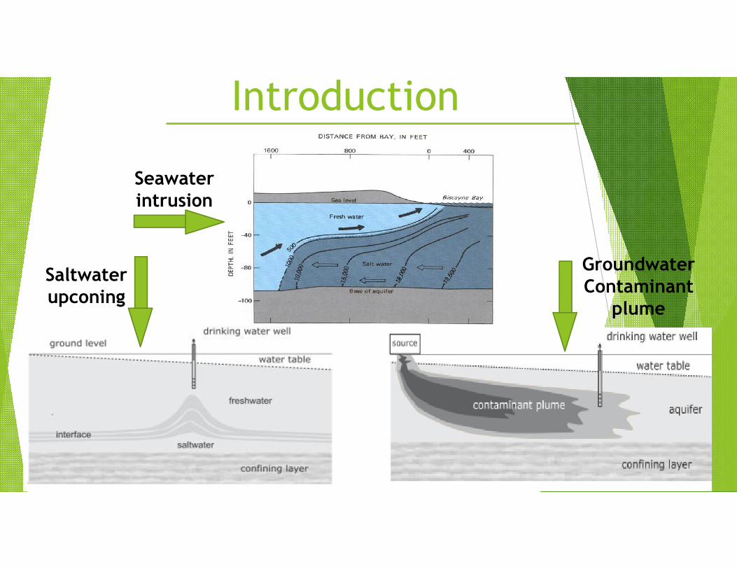
Introduction
kjhb
Seawater intrusion
Saltwater upconing
Groundwater Contaminant
plume
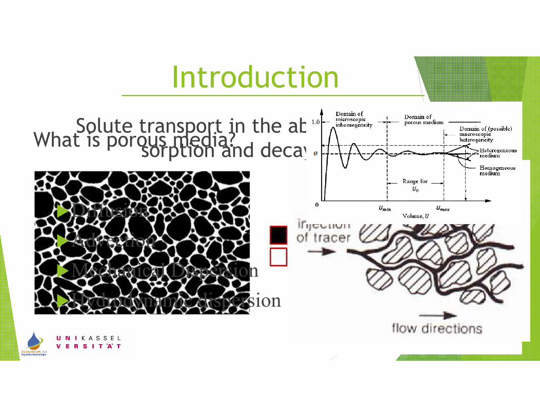
What is porous media?Solute transport in the absence of
sorption and decay:
Diffusion
Advection
Mechanical Dispersion
Hydrodynamic dispersion
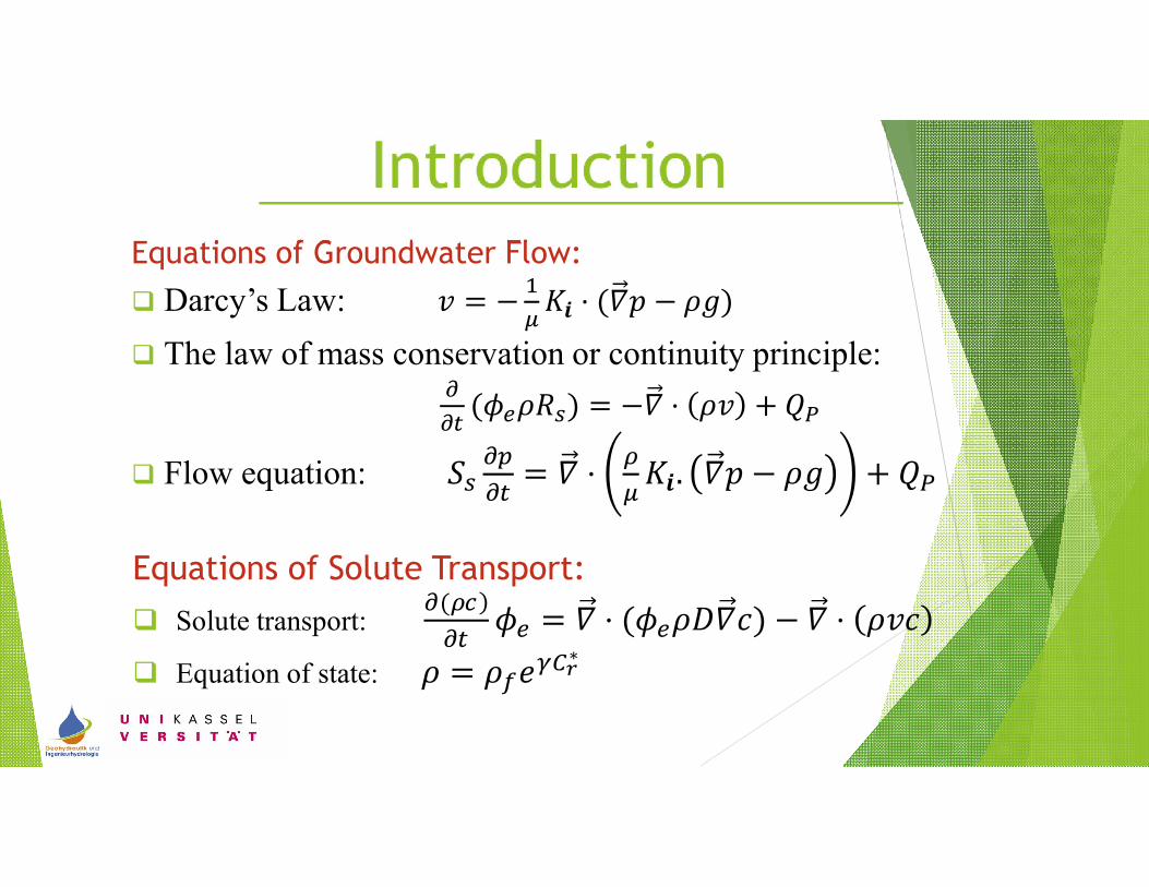
Equations of Groundwater Flow:
Darcy’s Law: � = −�
��� ⋅(�� − ��)
The law of mass conservation or continuity principle:�
��(�����)= −� ⋅ �� + ��
Flow equation: ����
��= � ⋅
�
���. �� − �� + ��
Equations of Solute Transport:
Solute transport: �(��)
���� = � ⋅(���� ��)− � ⋅ ���
Equation of state: � = ������∗

Dependency of transverse dispersion:
Dependency on fluid velocity by Peclet number
�� =��
�� ��= 0.28(��)�.����
�
Dependency on variable density
Dependency on heterogeneity
Dependency on scale

Literature Review
Investigator Year Research Work
Henry 1964
resolving the difficulties of modeling the
narrow transition zone between outflowing
fresh water and inflowing salt water
Kobus and Spitz 1985
Studying the quantitative evaluation of the
effects of permeability heterogeneity
interacting with density coupling
Schincariol and Schwartz 1990
illustrating the combined effect of
heterogeneity and solute concentration on
the vertical transvers e dispersion of a
continuously injected plume sinking in a
model aquifer
Investigator Year Research Work
Welty and Gelhar 1991, 1992
Finding that downward solute movement
due to gravity can enhance effective
vertical mixing or dispersion of a solute
plume
Tchelepi 1994
Finding that for fluids which also contrast
in density as well as viscosity, the tendency
of the overriding of the lighter fluid above
the less dense displaced one is damped by
permeability heterogeneity
Gleick et al. 2000
Investigating that global warming can be
expected to exacerbate seawater intrusion
into freshwater aquifers
Starke 2005
Studying the effect of heterogeneity on
density dependent transport in tank
experiment
Investigator Year Research Work
Schotting and
Gutierrez2008
Their investigation deals with the interplay of flow and transport
processes that affect dispersion. They found the fact that transverse
dispersivity was to be dependent on fluid velocity and density
difference contradicts the premise that dispersivity is a porous
medium constant.
Raoof and
Hassanizadeh2013
They did research about dispersivity dependence on saturation. In
this study, using a pore network model, they studied how the
transverse dispersivity varies nonlinearly with saturation. They
schematize the porous medium as a network of pore bodies and pore
throats with finite volumes to mimic the microstructure of real
porous media.
Karadimitriou et
al.2014
They did simultaneous thermal and optical imaging of two-phase
flow in a micro-model of the aquifer. They found that thermal
effects increase the dispersivity.
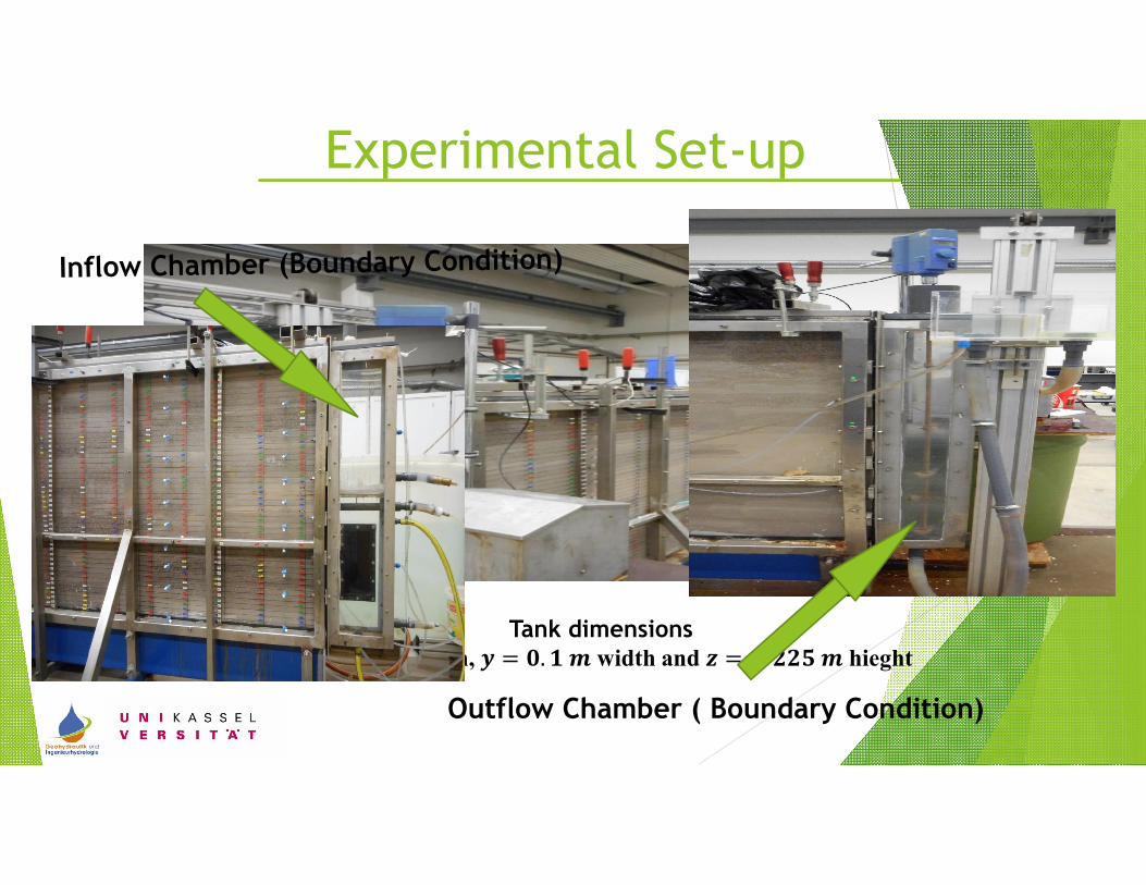
Experimental Set-up
Tank dimensions� = �.� � length, � = �.� � width and � = �.��� � hieght
Outflow Chamber ( Boundary Condition)

Schematic view of the Tank
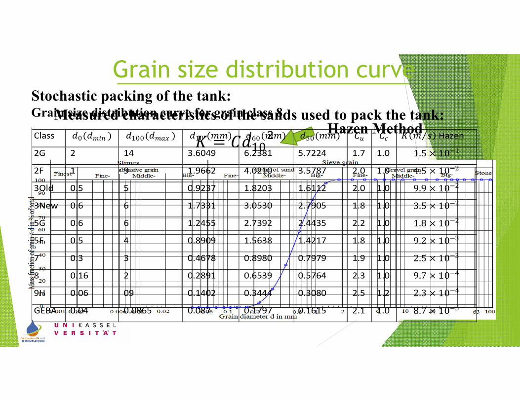
Grain size distribution curveStochastic packing of the tank: Grain size distribution curve for grain class 8.
� = ����� Hazen Method
Measured characteristics of the sands used to pack the tank:Class �0(���� ) �100(���� ) �10 (��) �60(��) �50(��) �� �� �(� �⁄ ) Hazen
2G 2 14 3.6049 6.2381 5.7224 1.7 1.0 1.5 × 10⁻¹
2F 1 9 1.9662 4.0210 3.5787 2.0 1.0 4.5 × 10⁻²
3Old 0.5 5 0.9237 1.8203 1.6112 2.0 1.0 9.9 × 10⁻²
3New 0.6 6 1.7331 3.0530 2.7905 1.8 1.0 3.5 × 10⁻²
5G 0.6 6 1.2455 2.7392 2.4435 2.2 1.0 1.8 × 10⁻²
5F 0.5 4 0.8909 1.5638 1.4217 1.8 1.0 9.2 × 10⁻³
7 0.3 3 0.4678 0.8980 0.7979 1.9 1.0 2.5 × 10⁻³
8 0.16 2 0.2891 0.6539 0.5764 2.3 1.0 9.7 × 10⁻⁴
9H 0.06 09 0.1402 0.3444 0.3080 2.5 1.2 2.3 × 10⁻⁴
GEBA 0.04 0.0865 0.087 0.1797 0.1615 2.1 1.0 8.7 × 10⁻⁵
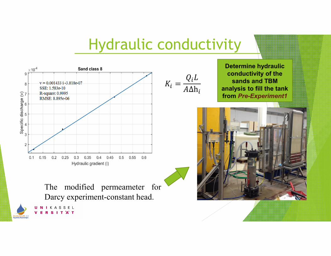
Hydraulic conductivityDetermine hydraulic conductivity of the
sands and TBM analysis to fill the tankfrom Pre-Experiment1
The modified permeameter forDarcy experiment-constant head.
�� =���
�Δh�
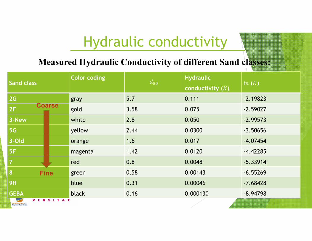
Measured Hydraulic Conductivity of different Sand classes:
Sand classColor coding
���Hydraulic
conductivity (�)�� (�)
2G gray 5.7 0.111 -2.19823
2F gold 3.58 0.075 -2.59027
3-New white 2.8 0.050 -2.99573
5G yellow 2.44 0.0300 -3.50656
3-Old orange 1.6 0.017 -4.07454
5F magenta 1.42 0.0120 -4.42285
7 red 0.8 0.0048 -5.33914
8 green 0.58 0.00143 -6.55269
9H blue 0.31 0.00046 -7.68428
GEBA black 0.16 0.000130 -8.94798
Hydraulic conductivity
Coarse
Fine
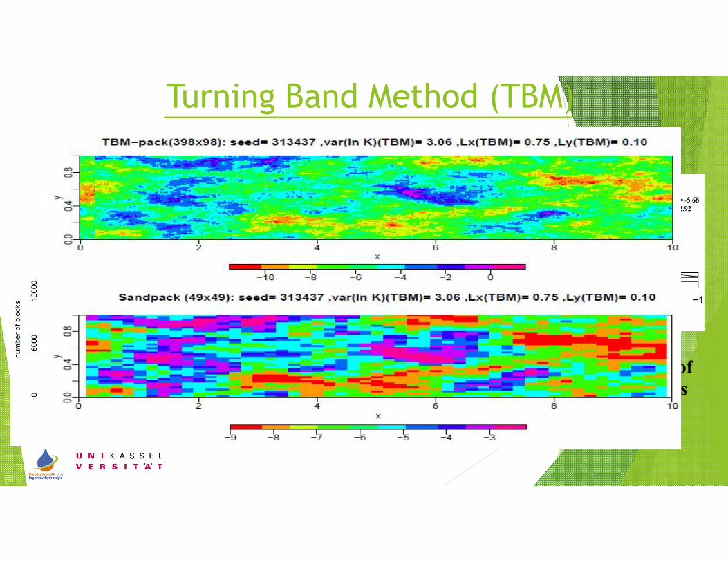
Turning Band Method (TBM)
Histogram of TBM blocks 392*98
Histogram of downscaled version of 392 × 98 blocks into 49 × 49 blocks
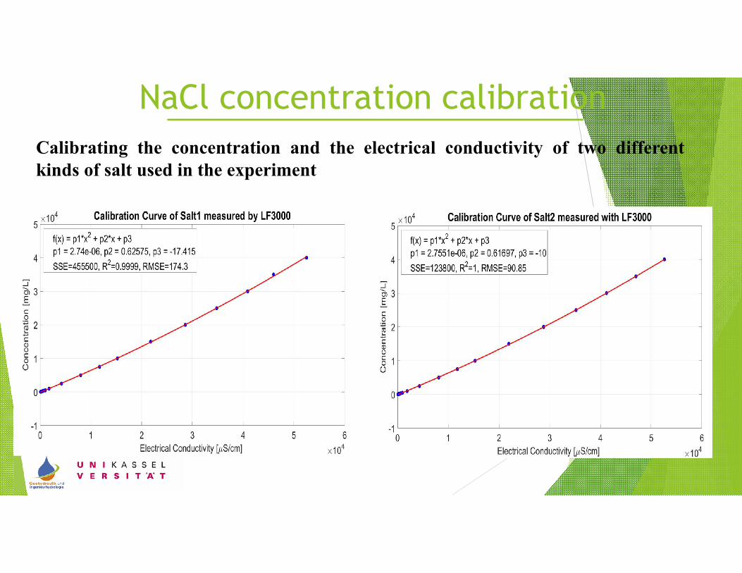
Calibrating the concentration and the electrical conductivity of two differentkinds of salt used in the experiment
NaCl concentration calibration
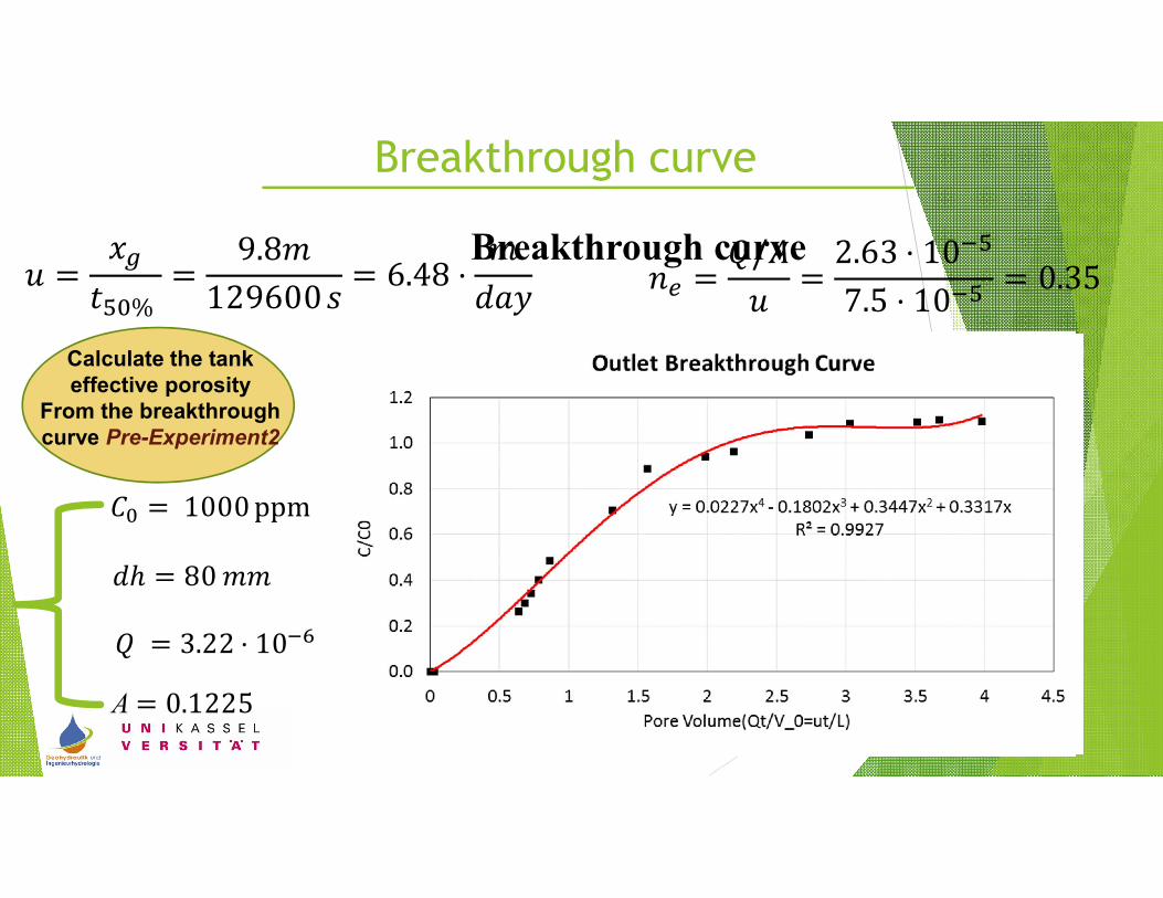
Breakthrough curve
�� = 1000 ppm
�ℎ = 80 ��
� =��
���% =
9.8�
129600 �= 6.48 ⋅
�
���
Breakthrough curve�� =
�/�
�=
2.63 ⋅10��
7.5 ⋅10��= 0.35
� = 3.22 ⋅10��
Piston flow:without molecular diffusionand mechanical dispersion
A = 0.1225
Calculate the tank effective porosity
From the breakthrough curve Pre-Experiment2
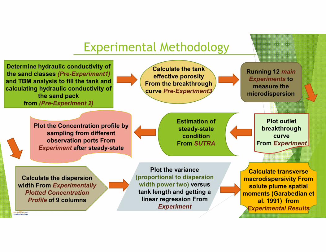
Experimental Methodology
Determine hydraulic conductivity of the sand classes (Pre-Experiment1) and TBM analysis to fill the tank and calculating hydraulic conductivity of
the sand packfrom (Pre-Experiment 2)
Calculate the tank effective porosity
From the breakthrough curve Pre-Experiment3
Running 12 main Experiments to
measure the microdispersion
Plot outlet breakthrough
curveFrom Experiment
Estimation of steady-state
conditionFrom SUTRA
Plot the Concentration profile by sampling from different observation ports From
Experiment after steady-state
Calculate the dispersion width From Experimentally
Plotted Concentration Profile of 9 columns
Plot the variance (proportional to dispersion
width power two) versus tank length and getting a linear regression From
Experiment
Calculate transverse macrodispersivity From
solute plume spatial moments (Garabedian et
al. 1991) from Experimental Results
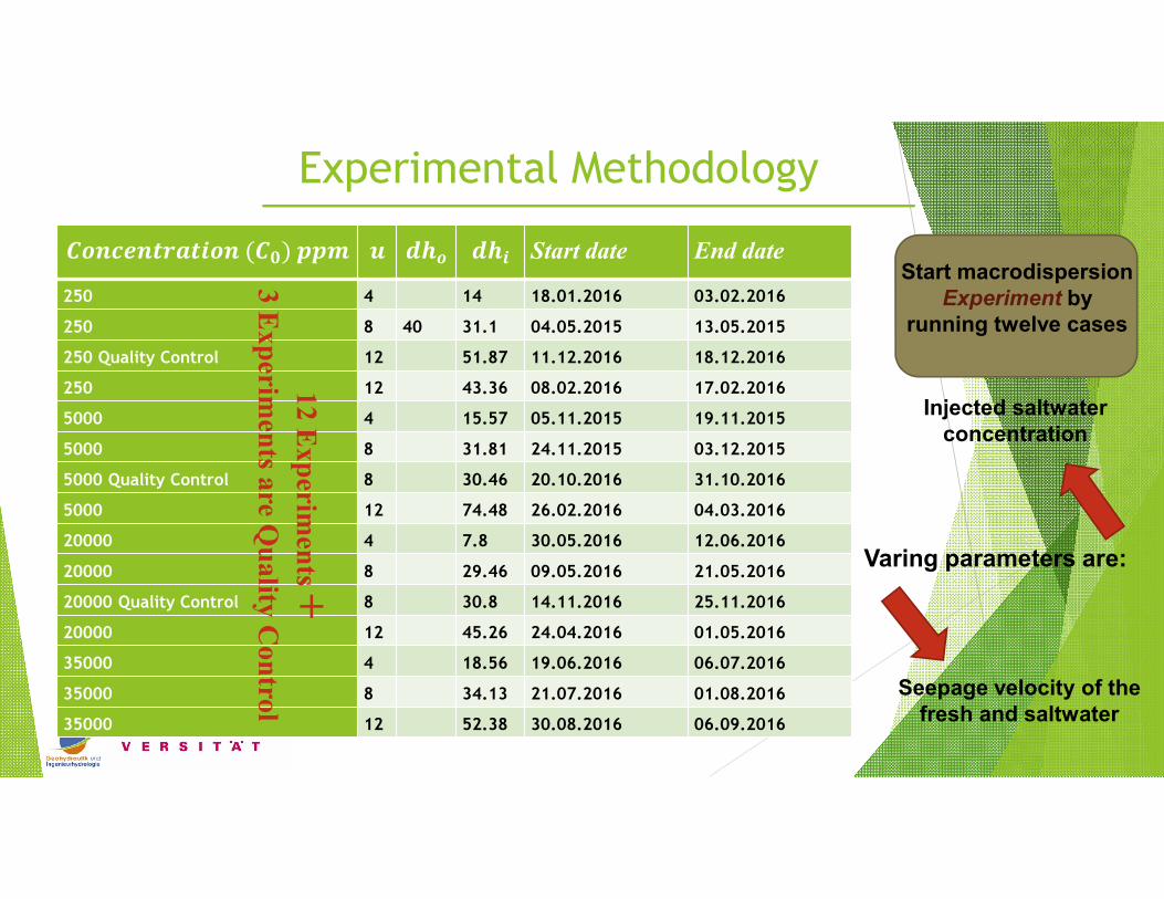
������������� (��) ��� � ��� ��� Start date End date
250 4 14 18.01.2016 03.02.2016
250 8 40 31.1 04.05.2015 13.05.2015
250 Quality Control 12 51.87 11.12.2016 18.12.2016
250 12 43.36 08.02.2016 17.02.2016
5000 4 15.57 05.11.2015 19.11.2015
5000 8 31.81 24.11.2015 03.12.2015
5000 Quality Control 8 30.46 20.10.2016 31.10.2016
5000 12 74.48 26.02.2016 04.03.2016
20000 4 7.8 30.05.2016 12.06.2016
20000 8 29.46 09.05.2016 21.05.2016
20000 Quality Control 8 30.8 14.11.2016 25.11.2016
20000 12 45.26 24.04.2016 01.05.2016
35000 4 18.56 19.06.2016 06.07.2016
35000 8 34.13 21.07.2016 01.08.2016
35000 12 52.38 30.08.2016 06.09.2016
Experimental Methodology
Varing parameters are:
Injected saltwater concentration
Seepage velocity of the fresh and saltwater
Start macrodispersionExperiment by
running twelve cases
12 E
xperim
ents +
3 E
xperim
ents are Q
uality
Co
ntrol
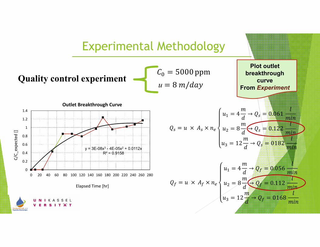
Experimental Methodology
Plot outlet breakthrough
curveFrom Experiment
y = 3E-08x3 - 4E-05x2 + 0.0112xR² = 0.9158
0
0.2
0.4
0.6
0.8
1
1.2
1.4
0 20 40 60 80 100 120 140 160 180 200 220 240 260 280
C/C
_exp
ecte
d [
]
Elapsed Time [hr]
Outlet Breakthrough Curve
�� = � × �� × ��
�� = 4�
�→ �� = 0.061
�
���
�� = 8�
�→ �� = 0.122
�
���
�� = 12�
�→ �� = 0182
�
���
�� = � × �� × ��
�� = 4�
�→ �� = 0.056
�
���
�� = 8�
�→ �� = 0.112
�
���
�� = 12�
�→ �� = 0168
�
���
�� = 5000 ppm
u = 8 �/���Quality control experiment

Experimental Methodology
�� = 5000 ppm
u = 8 �/���Quality control experiment
Estimation of steady-state
conditionFrom SUTRA

Experimental Methodology
�� = 5000 ppm
u = 8 �/���Quality control experiment
Plot the Concentration profile by sampling from different
observation ports From Experiment
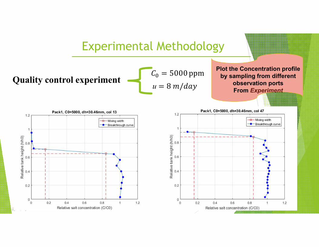
Experimental Methodology
�� = 5000 ppm
u = 8 �/���Quality control experiment
Plot the Concentration profile by sampling from different
observation ports From Experiment
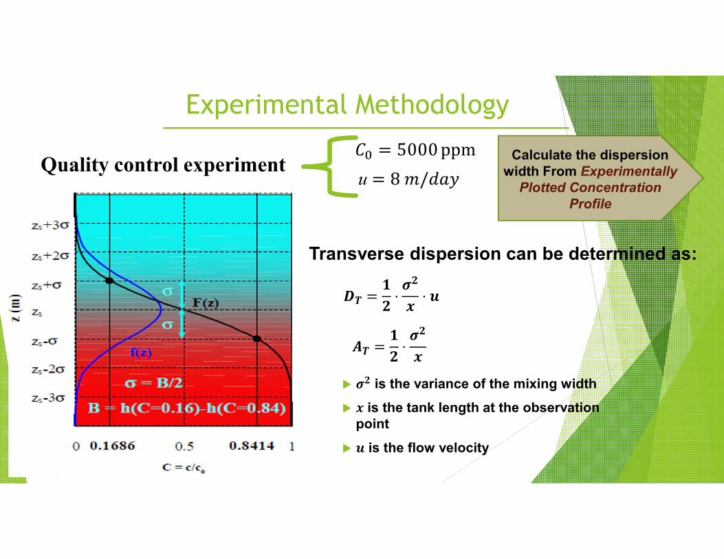
Experimental Methodology
�� = 5000 ppm
u = 8 �/���Quality control experiment
Calculate the dispersion width From Experimentally
Plotted Concentration Profile
�� is the variance of the mixing width
� is the tank length at the observationpoint
� is the flow velocity
�� =�
�⋅
��
�⋅�
�� =�
�⋅
��
�
Transverse dispersion can be determined as:
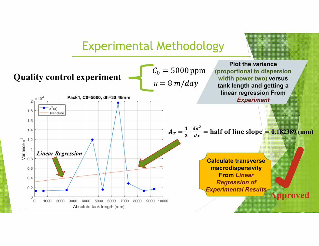
Experimental Methodology
�� = 5000 ppm
u = 8 �/���Quality control experiment
Plot the variance (proportional to dispersion
width power two) versus tank length and getting a linear regression From
Experiment
Calculate transverse macrodispersivity
From Linear Regression of
Experimental Results
�� =�
�⋅
���
��= ���� �� ���� ����� = 0.182389 (mm)
Linear Regression
Approved
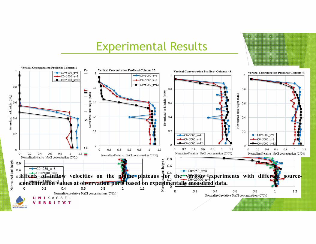
Experimental Results
Effects of inflow velocities on the plume plateaus for the various experiments with different source-concentration values at observation ports based on experimentally measured data.
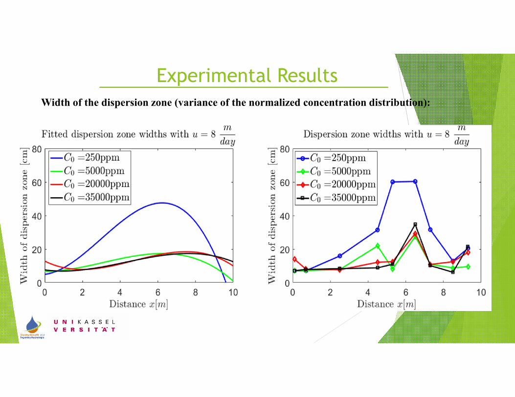
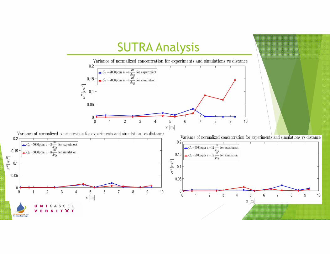
Experimental ResultsWidth of the dispersion zone (variance of the normalized concentration distribution):
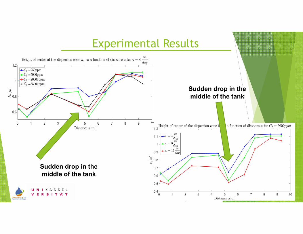
Experimental Results
Sudden drop in the middle of the tank
Sudden drop in the middle of the tank

Conclusions The transverse macrodispersivity was found to be proportional to the variance,
correlation length and anisotropy of the permeability distribution of the aquifer.
In the case of large molecular Peclet numbers, the diffusion is negligible, withlarge heterogeneity of the porous medium, as this work, the diffusion isnegligible. However, if the heterogeneity and the number of Peclet are small, thediffusion must be taken into account for the calculation.
The pressure distribution at the tank boundaries is a very sensitive parameter inthis model. Even slight deviations of the experimental conditions against thetheoretically determined pressure boundary conditions cause great changes in theflow and transport behavior of the system. The correct consideration andmaintenance of correct pressure boundary conditions is therefore indispensablefor an exact simulation of real processes.
Future works Experiments with variable granular structure dependent dispersivities �� and ��,
mean granular structure �� as well as attempts to study the homogeneous mediawhere influence of density is independent of the heterogeneity are necessary.
Because of the high pressure sensitivity at the boundaries of the model, anecessity of a continuous recording of the pressure levels using pressure probesis seen, which should be logged automatically.
In order to get the transport behavior data consistently everywhere in the tankand to prevent systematic errors, it’s reasonable to record the spatial andtemporal concentration process of water constituent (solute) with photometricand digital methods.

Thank you Vielen Dank
سپاسگزارم

Dependency of transverse dispersion:
Dependency on scaleHorizontal dispersivity Transverse dispersivity
Horizontal
Vertical
Longitudinal

Models of dispersion:
First order analysis
Perturbation analysis
Monte-Carlo analysis
This method was used in this work with Stochastic description ofhydraulic conductivity variation
comprehensive approach touncertainty propagation
deterministic solutions forthe numerically generatedrealizations

Piezometer boards
Two different Piezometerboards employed in differentstages of the experiment inorder to keep track of changesin the pressure inside andoutside of the tank.

Inlet Flowmeters
Flowmeters employed to track the flowrates of salt and freshwater at alltimes during the experiment to register an identical flowrate for both thefresh and salt water. The model of both flowmeters is Proline Promag 53,which operates based on electromagnetic fields.
Saltwater flowmeter
Freshwater flowmeter
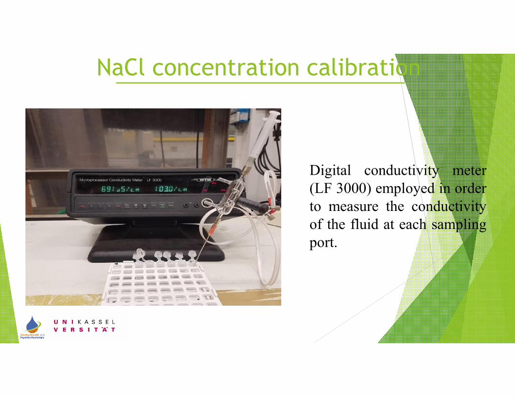
NaCl concentration calibration
Digital conductivity meter(LF 3000) employed in orderto measure the conductivityof the fluid at each samplingport.

Constant head method
Modified
The modified permeameter forDarcy experiment-constant head.

Experimental Tank Hydraulic Conductivity
�ℎ (��) �ℎ ∗ �/��� (
��
�) �(
�
�) �(
�
�) �� (
�
�) �� (
�
���)
5 6.250E-04 6.015E-06 9.624E-03 4.910E-05 1.228E-04 10.6064
10 1.250E-03 1.171E-05 9.371E-03 9.562E-05 2.391E-04 20.6544
12 1.500E-03 1.412E-05 9.412E-03 1.153E-04 2.881E-04 24.8951
14 1.750E-03 1.658E-05 9.474E-03 1.353E-04 3.384E-04 29.2345
16 2.000E-03 1.899E-05 9.493E-03 1.550E-04 3.875E-04 33.4797
Determination of the hydraulic conductivity of sand-pack:
� =� ⋅��
� ∙ �ℎ0
0.000002
0.000004
0.000006
0.000008
0.00001
0.000012
0.000014
0.000016
0.000018
0.00002
0.0005 0.0007 0.0009 0.0011 0.0013 0.0015 0.0017 0.0019 0.0021
Q (
m3
/day
)
dh*A/dl
A*dh/dl-Q
Plot of Discharge vs. Hydraulic Gradient:
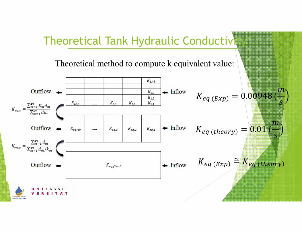
Theoretical method to compute k equivalent value:
��� (���) = 0.00948 (�
��
��� (������) = 0.01 (�
��
��� (���) =� ��� (������)
Theoretical Tank Hydraulic Conductivity
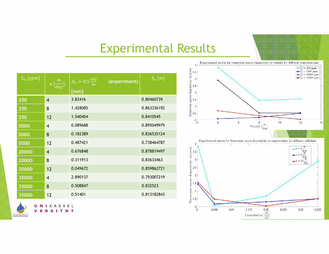
�� [���]� [
�
���] �� = 0.5
����
��(experiment)
[mm]
ℎ� [�]
250 4 3.83416 0.80460739
250 8 1.428085 0.863336192
250 12 1.540404 0.8410545
5000 4 0.089688 0.895049979
5000 8 0.182389 0.836535124
5000 12 0.487421 0.738464787
20000 4 0.676848 0.878819497
20000 8 0.311913 0.83633463
20000 12 0.049672 0.859862721
35000 4 2.890137 0.793007219
35000 8 0.508847 0.832523
35000 12 0.51401 0.813182843
Experimental Results
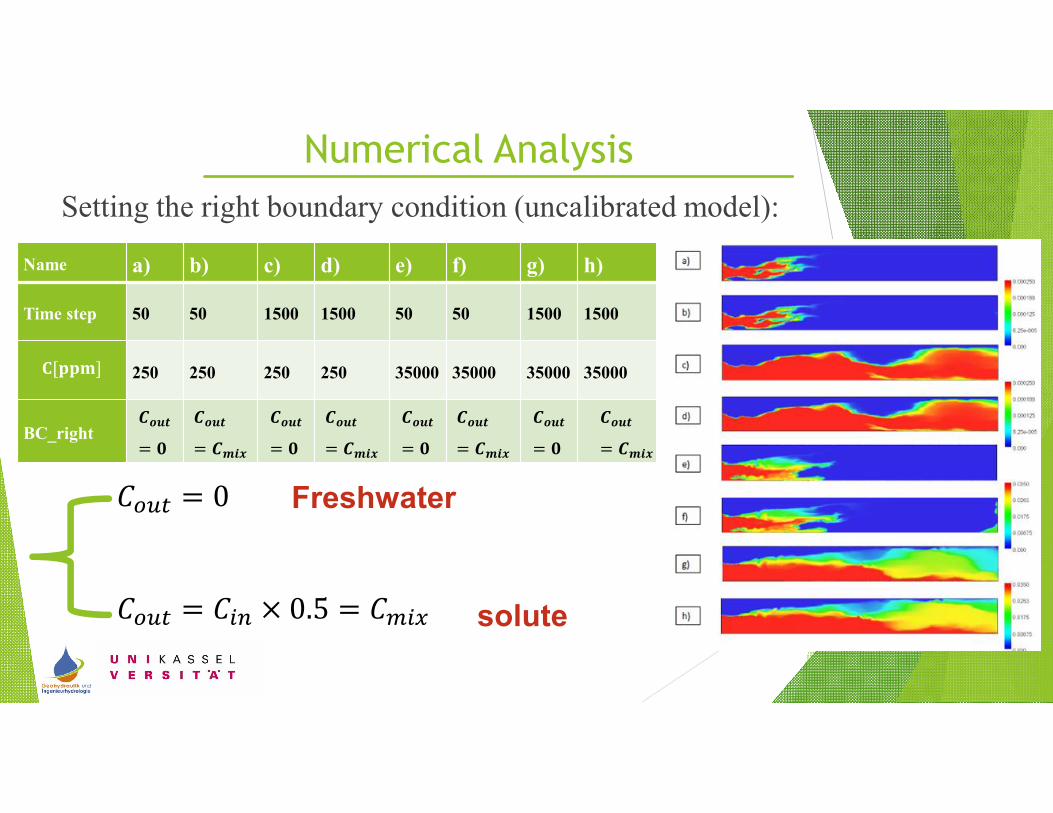
Numerical Analysis
Setting the right boundary condition (uncalibrated model):
Name a) b) c) d) e) f) g) h)
Time step 50 50 1500 1500 50 50 1500 1500
�[���] 250 250 250 250 35000 35000 35000 35000
BC_right����
= �
����
= ����
����
= �
����
= ����
����
= �
����
= ����
����
= �
����
= ����
���� = ��� × 0.5 = ����
���� = 0 Freshwater
solute
SUTRA Analysis

SUTRA Analysis
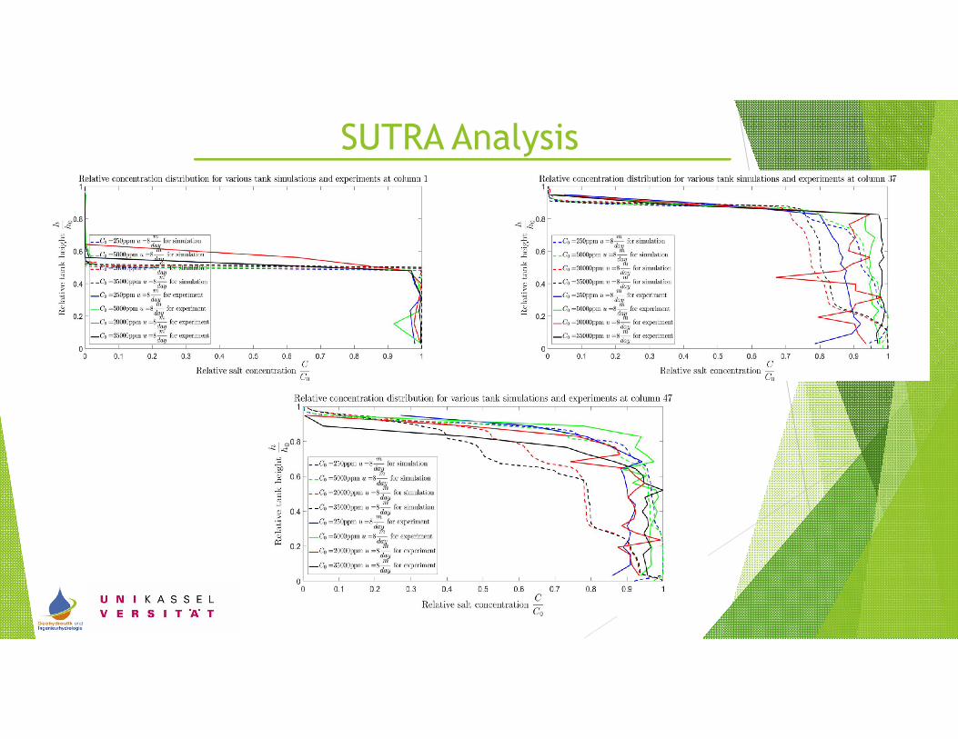
SUTRA Analysis
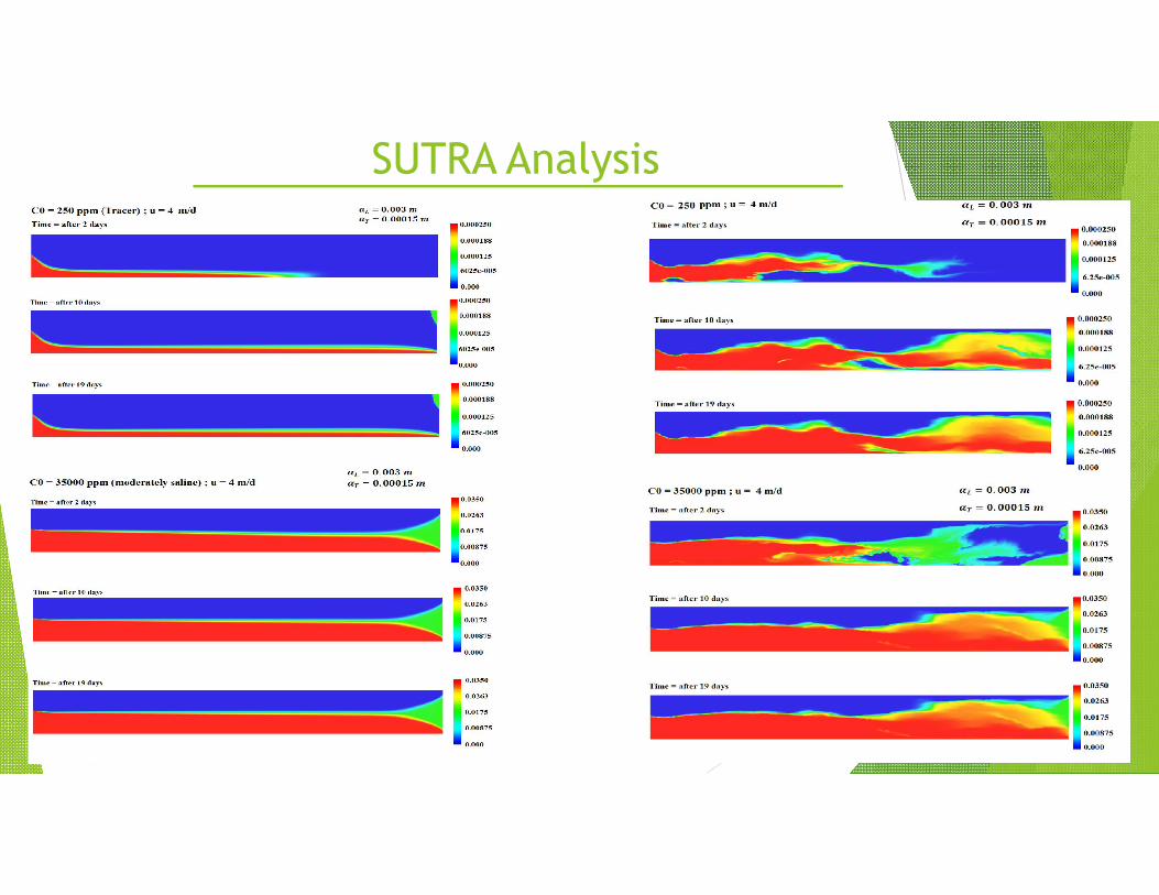
SUTRA Analysis
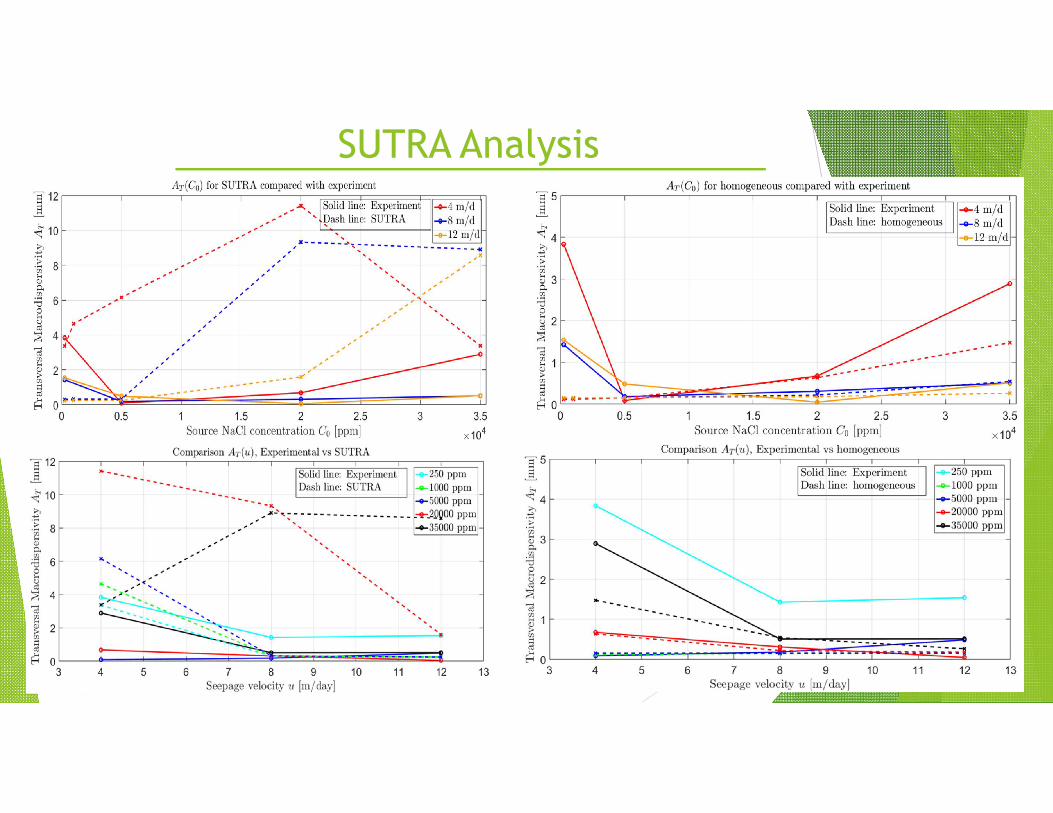
SUTRA Analysis
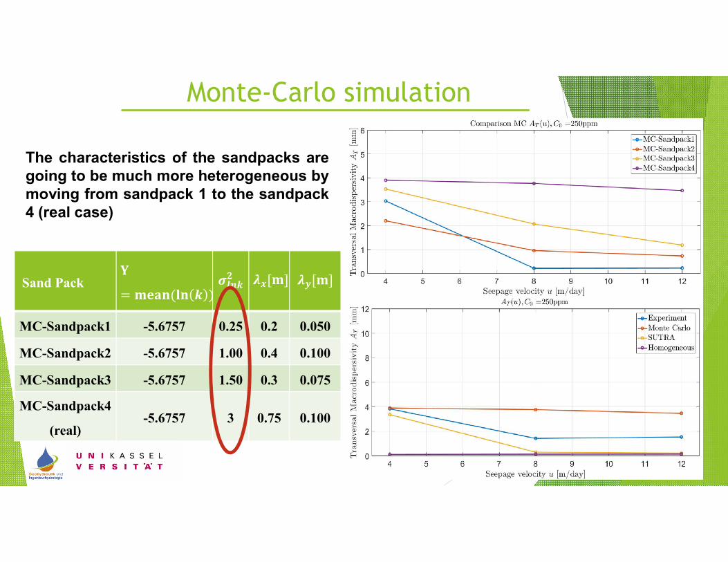
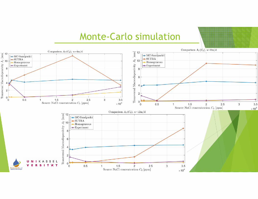
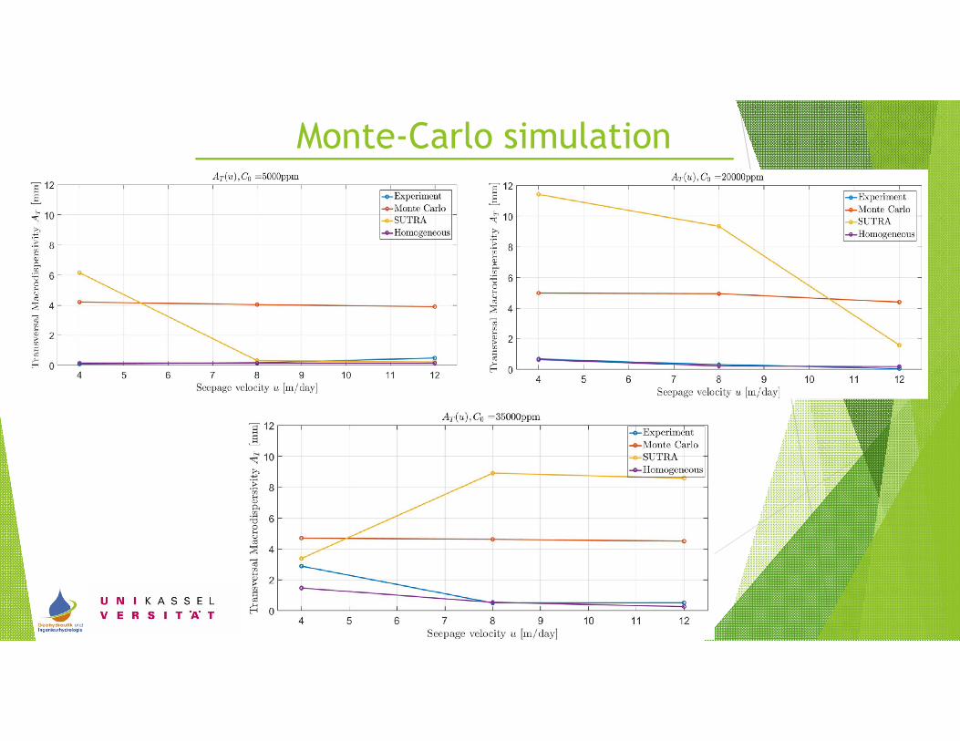
Monte-Carlo simulation
Sand Pack�
= ����(�� � )����
� ��[�] ��[�]
MC-Sandpack1 -5.6757 0.25 0.2 0.050
MC-Sandpack2 -5.6757 1.00 0.4 0.100
MC-Sandpack3 -5.6757 1.50 0.3 0.075
MC-Sandpack4
(real)-5.6757 3 0.75 0.100
The characteristics of the sandpacks aregoing to be much more heterogeneous bymoving from sandpack 1 to the sandpack4 (real case)
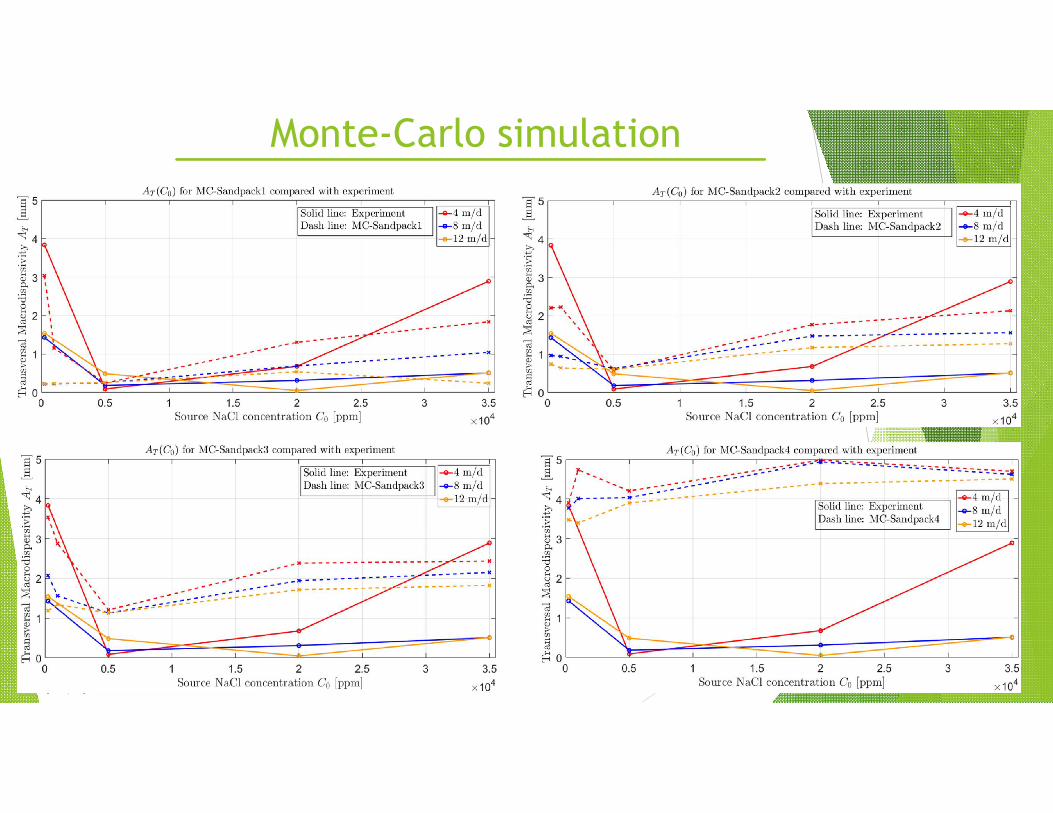
Monte-Carlo simulation

Monte-Carlo simulation
Monte-Carlo simulation
Monte-Carlo simulation