OPTIMAL DESIGN OF A SEGWAY - University of...

OPTIMAL DESIGN OF A SEGWAY By

Vijay Manikandan Janakiraman Taylor Tappe Hao Pan

Saradhi Rengarajan

ME 555-10-06 Winter 2010 Final Report

ABSTRACT

The system under consideration is a Segway human transport system. The Segway is a “two-wheeled, self-balancing electric vehicle,” which makes personal mobility easy and fun. The aim of this project is to optimize the Segway system to minimize the overall weight subjected to constraints on cost, performance, passenger comfort and stability. The Segway system has been divided into four key subsystems, namely, the structure, the electrical system, vibrations, and controls. Each subsystem is optimized to minimize its own objective function subjected to its own constraints and finally they are integrated and optimized as a system. The project describes the physics of each subsystem, the interaction between subsystems, and optimization at the subsystem and at a system level. Several insights have been gained on system modeling for optimization, model reduction and analysis, applying the theory behind optimization to practical problems, identifying the merits and demerits of different optimization algorithms, troubleshooting and selecting the best approach for the system problem etc. The project terminates by finding an optimal design which is more robust and a cost effective system comparable to the ones in the market.

2

Table of Contents

List of Figures ............................................................................................................................................... 7

List of Tables .............................................................................................................................................. 10

1. Design Problem Statement ..................................................................................................................... 13

1.1 Introduction ...................................................................................................................................... 13

1.2 Problem Statement ............................................................................................................................ 13

1.3 Model Assumptions and Approximations ........................................................................................ 14

1.4 System Quantities ............................................................................................................................. 15

1.4.1 List of Design Variables ............................................................................................................ 15

1.4.2 List of Parameters ...................................................................................................................... 16

1.4.3 List of Constants ........................................................................................................................ 18

1.5 Modeling Technique ......................................................................................................................... 18

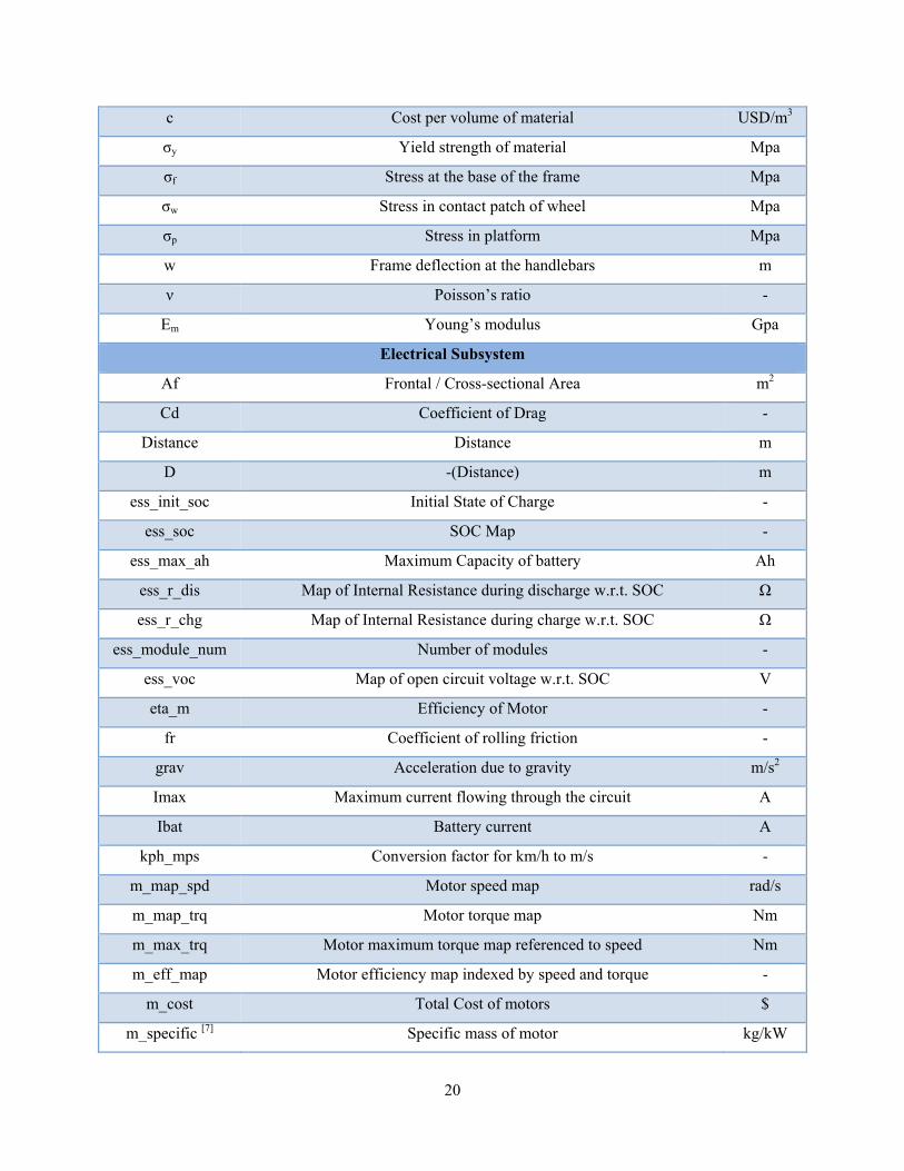
2. Nomenclature .......................................................................................................................................... 19

3. Structure Subsystem ................................................................................................................................ 24

3.1 Introduction ...................................................................................................................................... 24

3.2 Mathematical Model ......................................................................................................................... 26

3.2.1 Objective Function .................................................................................................................... 26

3.2.2 Constraints ................................................................................................................................. 28

3.2.3 Design Variables and Parameters .............................................................................................. 29

3.3 Model Analysis ................................................................................................................................. 30

3.3.1Monotonicity Analysis ............................................................................................................... 30

3.3.2 Behavior of Objective Function and Constraints ...................................................................... 32

3.4 Optimization Study ........................................................................................................................... 36

3.5 Parametric Study ............................................................................................................................... 37

3.6 Discussion of Results ........................................................................................................................ 38

3.7 System Trade-offs ............................................................................................................................. 40

4 Electrical Subsystem ................................................................................................................................ 41

3

4.1. Introduction ..................................................................................................................................... 41



4.2.2 Constraints ................................................................................................................................. 42

4.2.3 Governing Equations ................................................................................................................. 42

4.2.4 Model Summary ........................................................................................................................ 43

4.2.5 Coding for Numerical Processing: ............................................................................................ 43

4.3 Model Analysis ................................................................................................................................. 44

4.3.1 Monotonicity Analysis: ............................................................................................................. 44

4.3.2 Well-Boundedness: ................................................................................................................... 46


4.4.1 Optimizer Settings ..................................................................................................................... 46

4.4.2 Results and Possible Local Minima .......................................................................................... 47



4.7 System Trade-offs ............................................................................................................................. 49

5 Vibrations Subsystem .............................................................................................................................. 50

5.1 Introduction ...................................................................................................................................... 50


5.2.1 Description of the System ......................................................................................................... 50


5.2.3 Constraints ................................................................................................................................. 51

5.2.4 Model Summary ........................................................................................................................ 52

5.3 Model Analysis ................................................................................................................................. 54

5.3.1 Monotonicity Analysis .............................................................................................................. 54

5.3.2 Constraints Activity ................................................................................................................... 55

5.3.3 Well-boundedness ..................................................................................................................... 58

4


5.4.1 Approach 1: Changing Starting Points ...................................................................................... 58

5.4.2 Approach 2: Normalization and Changing DiffMinChange ..................................................... 60

5.4.3 Approach 3: Combining fmincon and Nomad .......................................................................... 61

5.4.4 Summary ................................................................................................................................... 61


5.5.1 Transmissibility vs F_0 ............................................................................................................. 63

5.5.2 Transmissibility vs m_S ............................................................................................................ 63


5.7 System-level Tradeoffs ..................................................................................................................... 65

6 Control System and Stability ................................................................................................................... 66

6.1 Introduction ...................................................................................................................................... 66

6.6.1 Subsystem Problem Statement .................................................................................................. 66



6.2.2 Plant Model ............................................................................................................................... 68

6.2.3 Design Variables and Parameters .............................................................................................. 69

6.3 Model Analysis ................................................................................................................................. 70

6.3.1 Behavior of objective function and constraints ......................................................................... 70

6.3.2 Monotonicity Table ................................................................................................................... 78


6.4.1 Optimization using FMINCON ................................................................................................. 80

6.4.2 Optimization using DIRECT METHOD and Combined Optimization .................................... 83


6.5.1 Passenger Mass ......................................................................................................................... 85

6.5.2 Passenger Height ....................................................................................................................... 86


5

6.7 System-Level Tradeoffs ................................................................................................................... 89

7 System Integration Study ......................................................................................................................... 91

7.1 System Interactions ........................................................................................................................... 91

7.2 Problem Formulation ........................................................................................................................ 92

7.3 Optimization Approaches ................................................................................................................. 95

7.3.1 First Attempt with fmincon ....................................................................................................... 95

7.3.2 Direct Method Algorithm .......................................................................................................... 97

7.3.3 Nomad Algorithm ..................................................................................................................... 98

7.3.4 Simulated Annealing ................................................................................................................. 98

7.3.5 Sequential Aptimization of Subsystems .................................................................................... 98

7.3.6 Second Attempt with fmincon ................................................................................................... 99

7.4 Numerical Results ........................................................................................................................... 100

7.5 Conclusion ...................................................................................................................................... 102

8. References ............................................................................................................................................. 103

9. Appendix ............................................................................................................................................... 105

9.1 Structrural Subsystem ..................................................................................................................... 105

9.1.1 MATLAB Codes ..................................................................................................................... 105

9.2 Electrical Subsystem ....................................................................................................................... 110

9.2.1 MATLAB Codes ..................................................................................................................... 110

9.2.2 SIMULINK Blocks ................................................................................................................. 112

9.3 Vibrations Subsystem ..................................................................................................................... 115

9.3.1 Methods Comparison .............................................................................................................. 115

9.3.2 MATLAB codes ...................................................................................................................... 116

9.3.3 Nomad Codes .......................................................................................................................... 118

9.3.4 Derivation of Governing Equations of the System.................................................................. 119

9.3.5 Unsuccessful Attempts in the Optimization Process ............................................................... 121

9.4 Controls Subsystem ........................................................................................................................ 123

6

9.4.1 Direct Method Codes .............................................................................................................. 123

9.4.2 MATLAB Codes ..................................................................................................................... 125

7

List of Figures

Figure 1.1 A real segway pircture

Figure 3.1 Segway model view 1


Figure 3.4 Wheel stress vs wheel radius

Figure 3.5 Objective function vs wheel thickness

Figure 3.6 Wheel stress vs wheel thickness

Figure 3.7 Contact fraction vs wheel thickness

Figure 3.8 Objective function vs platform thickness

Figure 3.9 Objective function vs platform length

Figure 3.10 Platform stress vs platform length

Figure 3.11 Objective function vs platform width

Figure 3.12 Platform stress vs platform width

Figure 3.13 Contact fraction vs platform width

Figure 3.14 Objective function vs Outer frame diameter

Figure 3.15 Pipe stress vs outer frame diameter

Figure 3.16 Frame deflection vs outer diameter

Figure 3.17 Objective function vs frame diameter

Figure 3.18 Pipe stress vs frame diameter

Figure 3.19 Frame deflection vs inner diameter

Figure 3.20 Objective function handlebar height

Figure 3.21 Pipe stress vs handlebar height

Figure 3.22 Frame deflection vs handlebar height

8

Figure 3.23 Objective function vs. iteration

Figure 3.24 System mass vs load

Figures 3.25-27 Structural subsystem optimized design model, view 1 and view 2

Figure 4.1 Parametric study: required maximum speed

Figure 5.1 Vibrations subsystem mathematical model

Figure 5.2 Transmissibility vs c_S

Figure 5.3 Transmissibility vs c_T

Figure 5.4 Transmissibility vs k_S

Figure 5.5 Transmissibility vs k_T

Figure 5.6 Transmissibility vs m_T

Figure 5.7 Nomad: objective functions vs iterations for different sets of starting points

Figure 5.8 Transmissibility vs F_0

Figure 5.9 Transmissibility vs m_S

Figure 6.1 Segway System sketch [5]

Figure 6.2 SIMULINK model of the feedback system

Figure 6.3 Effect of variable X1 on objective and constraints





Figure 6.8 Optimization progress for CASE 1


9


Figure 6.11 Working principle behind global optimization (Direct) and local optimization (fmincon)

Figure 6.12 Variation of settling time with Passenger Mass

Figure 6.13 Variation of system constraints with Passenger Mass

Figure 6.14 Variation of Settling time with Passenger center of mass height

Figure 6.15 Variation of constraints with Passenger center of mass height

Figure 6.16 Summary of optimization study

Figure 6.17 Comparison of optimal controller to that of the base controller

Figure 7.1 System interactions

Figure 7.2 fmincon: objective function vs iteration

Figure 7.3 fmincon: objective function vs iterations

Figure 7.4 fmincon: objective function with iterations

Figure 9.1 Main block

Figure 9.2 Electric motor block

Figure 9.3 Battery block

Figure 9.4 Pack Voc, Rint block

Figure 9.5 Current computation block

Figure 9.6 SOC algorithm block

10

List of Tables

Table 1.1 Segway subsystems and corresponding responsible persons

Table 1.2 List of design variables

Table 1.3 List of parameters

Table 1.4 List of constants

Table 2.1 Nomenclature

Table 3.1 Structural subsystem constraints

Table 3.2 Structural subsystem monotonicity table

Table 3.3 Structural subsystem typical values of parameters

Table 3.4 Optimum for carbon fiber

Table 3.5 Numerical results of the parametric study with respect to material

Table 3.6 Parametric study on different materials and corresponding optimum

Table 4.1 Electrical subsystem design variables

Table 4.2 Electrical subsystem parameters

Table 4.3 Bounds of the design variables

Table 4.4 Optimizer settings

Table 4.5 Optimization results

Table 4.6 Parametric study: required maximum speed

Table 5.1 Vibrations subsystem design variables

Table 5.2 Vibrations subsystem parameters

Table 5.3 Vibrations subsystem constant

Table 5.4 Vibrations subsystem constraints

Table 5.5 Nomad optimization results

11

Table 5.6 Summary of constraint activity

Table 5.7 Different sets of starting points

Table 5.8 Nomad optimization results for different sets of starting points

Table 5.9 fmincon results for different sets of starting points

Table 5.10 Combining Nomad and fmincon: results for different sets of starting points

Table 5.11 Summary of optimization results

Table 6.1 System constraints and description

Table 6.2 Effect of variable X1 on objective and constraints





Table 6.7 Monotonicity Table

Table 6.8 System Parameters and Constants

Table 6.9 Comparison of fmincon optimization routine for different initial conditions

Table 6.10 Comparison of fmincon and direct method optimization routines

Table 7.1 Transformation of roles of subsystems

Table 7.2 Showing feasible design and the objective corresponding to it

Table 7.3 Comparing the feasible design and the sequential optimum objective functions

Table 7.4 Comparing the objective function values of the feasible design, the sequential optimum and the

fmincon solution from sequential optimum

Table 7.5 Listing the optimal design at the system and the subsystem levels

Table 7.6 Listing the objective function values at the system and the subsystem levels

12

Table 7.7 Summary of final costs

Table 9.1 Method comparison

Table 9.2 fmincon: results

13

1. Design Problem Statement

1.1 Introduction

The Segway Human Transport system is a personal transport vehicle used for short commutes. It

has zero emissions and is estimated to cost around 2.5 cents in electricity bills per hour of operation. The

Segway works on balancing on an inverted pendulum concept where the user gives a small disturbance by

tilting forward (the intended direction of motion) and the platform responds by moving in that direction to

balance the passenger from falling which gives a constant velocity along that direction. This can be

extended to motion in all directions on the horizontal plane, i.e., just by simply shifting the passenger’s

center of mass, the Segway is steered along the required direction. The segways available in the market

can travel up to a speed of 12.5 mph and occupy a footprint width that is only slightly larger than the

shoulder width of an average person.

Figure 1.1 A real Segway picture [1]

1.2 Problem Statement

The system objective is to minimize the mass of the segway system which can be stated as

follows:

, , ,

, ; … 1.1

14

The objective function above was subjected to the subsystem and system level constraints. There

were several performance quantities that qualified for the system objective but the mass of the overall

system was taken as the objective function and the others were treated as constraints. The primary reason

was to reduce the model complexity by avoiding multiple objectives and weighted objective function. The

mass was chosen over another viable candidate, cost because an accurate inclusive cost model was

difficult to obtain. Furthermore, cost and mass are closely related and mass was chosen over cost in order

to have a more accurate representation of the problem. Also, optimizing for mass would result in other

advantages like user-friendliness, enhanced performance and greater usability.

The division of the Segway system and the team member responsible for each subsystem is as

follows:

Subsystem Team member

Structure and body design Taylor

Motor and battery performance Saradhi

Passenger comfort and vibrations Paul

Control and stability Vijay

Table 1.1 Segway subsystems and corresponding responsible persons

These four subsystems were chosen to represent the whole Segway for this optimization problem

because they well-represent the entire system while maintaining a level of complexity which is

appropriate for this project. For the specific objective, the structural optimization and the powertrain

optimization are supremely important. For the general functionality of the Segway, the control

optimization and the comfort/vibration optimization are crucial to making this model more realistic.

1.3 Model Assumptions and Approximations

The assumptions associated with the structural model include material and geometric

assumptions. For instance, the model treats the wheels, frame and platform separately and does not

account for the interactions between those components. Secondly, the entire structure was made of one

single material with a very low safety factor of 1.25, which, if changed would directly affect the mass of

the system. The handlebars dimensions were not modeled or included in the objective function in order to

reduce the model complexity. Lastly, the model assumes a concentrated load at the handlebars and

another concentrated load directly in the center of the plate. Further explanation of the model

assumptions can be located in the structural subsystem’s modeling section. The electrical system captures

15

the power relations between the motor and battery and no thermal model was included. Also the

dimensions of motor and battery were not considered in the model. The vibrations system only considered

the vibrations in the vertical direction while lateral and longitudinal motions were neglected. The

interactions between the wheels and the ground were generated based on equivalent spring and damping

effects of the wheels. The suspension system was assumed to be inserted between the wheels and the

segway platform and it was composed of only springs and dampers. The ground excitation was assumed

to be a sinusoidal wave since it is very common and easy to be described mathematically. Also tire mass

was neglected. The control system was modeled for longitudinal motion of the segway traveling at

maximum velocity. Steering and rolling was neglected. All dynamics were assumed continuous and a full

state feedback was assumed to be available for the controller. The weight of the controller and associated

power electronics were neglected.

1.4 System Quantities

The design variables of the system are a combination of the design variables for the subsystems.

Below is a list of variables, parameters and constants for the complete system.

1.4.1 List of Design Variables

No. Variable Units Upper

bound

Lower

Bound

Feasible

Design Description

Structural Subsystem

1 Material - - - Al 6061 Structural Material

2 r m 1 .1 .152 Wheel radius

3 t m 1 .01 .035 Wheel thickness

4 wp m 1 .1 .63 Platform width

5 hp m 1 .01 .035 Platform thickness

6 lp m 1 .1 .45 Platform length

7 dfi m 1 0 .084 Inner Frame diameter

8 dfo m 1 .001 .1 Outer Frame diameter

9 hh m 1.2 .1 .951 Handlebar height

Electrical Subsystem

10 sfm - 5 0.1 1 Scaling factor for motor

16

11 sbv - 5 0.1 2 Scaling factor for battery

voltage

12 sba - 5 0.1 1 Scaling factor for battery Ah

capacity

Vibrations Subsystem

13 c_S N*sec/m 5000 3000 4000 Damping coefficient of

suspension

14 c_T N*sec/m 1500 500 1000 Damping coefficient of the

wheels

15 k_S N/m 30000 10000 20000 Spring constant of suspension

16 k_T N/m 300000 200000 250000 Spring constant of the wheels

17 m_T kg 25 5 15 Mass of the wheels

Controls Subsystem

18 q1 - 100 1 34.449 Weight factor for state 1


20 q3 - 100 1 100 Weight factor for state 3


22 r - 1 0.01 0.01 Weight factor for controller

effort

Table 1.2 List of design variables

1.4.2 List of Parameters

No. Parameter Value Units Description


1 A 450 USD Maximum cost

2 B .1 m Minimum safety platform lip height

3 C .1 m Minimum Ground clearance

4 E .7 m Maximum device footprint width

5 F .5 m Maximum device footprint length

6 G .951 m Lowest handlebar height

7 H .08 m Human foot width

8 I .5 m Distance between medial sides of the foot

17

9 J .3 m Human foot length

10 K .4 m human step height

11 L 1.1898 m Highest handlebar height

12 Ph 300 N Maximum handlebar load

13 Pb 4000 N Maximum load at the platform

14 N .0005 m Maximum handlebar deflection

15 hm .05 m Typical motor height

16 ρ 2700 kg/m3 Density for Al 6061

17 c 11880 USD/m3 Cost for Al 6061

18 σy 275 MPa Yield strength

19 ν .33 - Poisson’s Ratio for Al 6061


20 vmax 20 km/h Maximum speed required

21 TR 20 - Transmission ratio

22 Rw 0.20 m Tire Radius

23 torque 6 Nm Torque requirement from user

24 Af 0.7 m2 Frontal Area of cross-section

25 Mv 150 kg Total mass (Segway + Payload)

26 ess_init_soc 0.9 - Initial SOC


27 F_0 0.1 N Magnitude of ground excitation

28 m_S 100 kg Total mass of the rider and segway excluding wheels

29 omega 60 Hz Frequency of ground excitation

30 t_S 0 sec Starting time of simulation

31 t_E 5 sec Ending time of simulation

32 V_S_S 0 m/sec Initial vertical velocity of the rider

33 V_T_S 0 m/sec Initial vertical velocity of the wheels

34 z_S_S 0 m Initial vertical displacement of the rider

35 z_T_S 0 m Initial vertical displacement of the wheels

Controls Subsystem

36 l 1.8 m Passenger height

37 m 120 Kg Passenger weight

18

Table 1.3 List of parameters

1.4.3 List of Constants

No. Parent subsystem Constant Value Units Description

1 Electrical Cd 0.7 - Coefficient of drag

2 Electrical rho 1.2 kg/m3 Density of air

3 Electrical fr 0.015 - Coefficient of rolling resistance

4 Controls, Vibrations and Electrical g 9.81 m/s2 Acceleration due to gravity

Table 1.4 List of constants

1.5 Modeling Technique

Most of the models for the subsystems were implicit (black box type) models except for the

structure subsystem which was modeled based on analytical relations. All the subsystems were modeled

in MATLAB and hence developing a system level model was merely making a connection between the

subsystems. The optimization was also done mainly using fmincon (an implementation of the sequential

quadratic programming algorithm). Other algorithms such as the direct method, nomad etc were also tried

and more information can be found in the later sections of this report.

38 V_max 12.5 Mph Maximum velocity

19

2. Nomenclature

Symbol Description Units


Structural Material Material used for body of Segway (steel, Al etc.) -

r Wheel radius m

t Wheel thickness (measured from lateral platform edge to lateral wheel

edge) m

wp Platform width m

hp Platform thickness m

lp Platform length m

dfi Inner frame diameter m

dfo Outer frame diameter m

hh Handlebar height m

A Structural cost (for structural components only) USD

B Distance from top of platform to tops of wheels m

C Ground clearance m

E Device footprint width m

F Device footprint length m

G Low height of human hand from bottom of foot m

H Human foot width m

I Distance between medial sides of feet m

J Human foot length m

K Human step height m

L High elbow height m

Ph Maximum handlebar load N

Pb Maximum base load N

N Maximum handlebar deflection m

hm Height of the motor and battery packs m

ρ Density of chosen material kg/m3

20

c Cost per volume of material USD/m3

σy Yield strength of material Mpa

σf Stress at the base of the frame Mpa

σw Stress in contact patch of wheel Mpa

σp Stress in platform Mpa

w Frame deflection at the handlebars m

ν Poisson’s ratio -

Em Young’s modulus Gpa


Af Frontal / Cross-sectional Area m2

Cd Coefficient of Drag -

Distance Distance m

D -(Distance) m

ess_init_soc Initial State of Charge -

ess_soc SOC Map -

ess_max_ah Maximum Capacity of battery Ah

ess_r_dis Map of Internal Resistance during discharge w.r.t. SOC Ω

ess_r_chg Map of Internal Resistance during charge w.r.t. SOC Ω

ess_module_num Number of modules -

ess_voc Map of open circuit voltage w.r.t. SOC V

eta_m Efficiency of Motor -

fr Coefficient of rolling friction -

grav Acceleration due to gravity m/s2

Imax Maximum current flowing through the circuit A

Ibat Battery current A

kph_mps Conversion factor for km/h to m/s -

m_map_spd Motor speed map rad/s

m_map_trq Motor torque map Nm

m_max_trq Motor maximum torque map referenced to speed Nm

m_eff_map Motor efficiency map indexed by speed and torque -

m_cost Total Cost of motors $

m_specific [7] Specific mass of motor kg/kW

21

Mv Total Mass of Segway (Vehicle + Payload) kg

N_tire Rotational Speed of tire rpm

N_motor Rotational Speed of motor rpm

Pbat Power requested from battery W

P_supplied Power supplied by battery to motor W

Pm Motor Power kW

Rw Radius of wheel m

Rint Net Internal Resistance Ω

rho Density of air kg/m3

sfm Scaling factor for motor sizing -

sbv Scaling factor for battery voltage -

sba Scaling factor for battery capacity -

soc State of Charge of battery at any instant -

TR Transmission Ratio -

torque Torque requirement from driver -

time Maximum time of simulation sec

used_ah Battery Capacity used Ah

vmax Required top speed km/h

v Actual speed output at wheels km/h

Voc Total Open Circuit Voltage V

Vbat Terminal Voltage of battery V

wm Mass of motor kg

wb Mass of battery pack kg

w Total mass of electrical system kg


c_S Damping coefficient of the suspension N*sec/m

c_T Damping coefficient of the wheels N*sec/m

F_0 Magnitude of ground excitation displacement z_G N

g Gravity m/sec2

k_S Spring constant of the suspension N/m

k_T Spring constant of the wheels N/m

m_S Total mass of the rider and the segway excluding the wheels kg

22

m_T Total mass of the two wheels kg

omega Frequency of ground excitation displacement z_G Hz

t Time sec

t_S Starting time of modeling dynamics of the segway system sec

t_E Ending time of modeling dynamics of the segway system sec

V_S_S Starting value of the vertical velocity of the segway rider m/sec

V_T_S Starting value of the vertical velocity of the tires m/sec

z_G Vertical displacement due to ground excitation m

z_S Vertical displacement felt by the segway rider m

z_S_S Starting value of vertical displacement felt by the segway rider m

z_T Vertical displacement of the tires m

z_T_S Starting value of vertical displacement of the tires m

xi Vector of starting points for the optimization, i=1,2,3,4 NA

Controls Subsystem

Segway frame tilt angle Radians

Segway frame angular velocity Rad/s

Segway platform displacement m

Segway platform velocity m/s

q1, q2, q3, q4 Weight values correspond to states , , , -constant-

r Weight corresponding to the control effort -constant-

Q Diagonal matrix containing the qi -constant-

R Diagonal matrix containing the r -constant-

M Segway system mass kg

m Passenger mass kg

l Distance of wheel centerline to the passenger center of mass m

Ei Eigen values of the system -constant-

Plant input or controller output. It is the command to the actuator

(motor command) N

Rise time s

Settling time s

% overshoot %

g Acceleration due to gravity m/s2

23

P Power of motor KW

N Speed of motor rpm

T Torque of motor Nm

K State feedback gain vector -constant

Table 2.1 Nomenclature

24

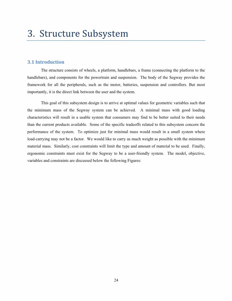
3. Structure Subsystem

3.1 Introduction

The structure consists of wheels, a platform, handlebars, a frame (connecting the platform to the

handlebars), and components for the powertrain and suspension. The body of the Segway provides the

framework for all the peripherals, such as the motor, batteries, suspension and controllers. But most

importantly, it is the direct link between the user and the system.

This goal of this subsystem design is to arrive at optimal values for geometric variables such that

the minimum mass of the Segway system can be achieved. A minimal mass with good loading

characteristics will result in a usable system that consumers may find to be better suited to their needs

than the current products available. Some of the specific tradeoffs related to this subsystem concern the

performance of the system. To optimize just for minimal mass would result in a small system where

load-carrying may not be a factor. We would like to carry as much weight as possible with the minimum

material mass. Similarly, cost constraints will limit the type and amount of material to be used. Finally,

ergonomic constraints must exist for the Segway to be a user-friendly system. The model, objective,

variables and constraints are discussed below the following Figures:

25



26

3.2 Mathematical Model

3.2.1 Objective Function

The goal of this subsystem is to minimizing the mass of the Segway while adhering to the

constraints of the problem. For this subsystem, minimizing mass translates to minimizing material of the

Segway and then performing a parametric study of the material to be used. Stress and deflection

constraints will be important as will practical usability issues. Multiple analytical expressions were used

for the stress and deflection constraints.

r, t, w , h , l , df , df , h , , , , , , , , , , , , , , , , , , , ,

The formulation above only realizes eight variables and includes all the material properties into

the parameters since the material choice is a discrete variable. The equations for the objective function

and intermediate parameters σf, σw, σp, and w are discussed below and must be calculated for the sake of

the constraints.

22 2

… 3.1

The objective function simply adds the volumes of the separate components: two wheels, a

platform and the frame, and multiplies the sum by the density of the chosen material.

32… 3.2

My model assumes a circular pipe loaded at one end (the handlebars) and fixed at the other (the

platform). This equation comes from beam theory and simply gives the maximum stress, which occurs at

the fixed end, in the pipe as a function of its dimensions and the load applied.

… 3.3

For the stress on the wheel, my model assumes uniform stress along the tire bead. This is not an

accurate model of the stress if no tire is used, and even then, it makes some rather large assumptions.

Without the tire, the stress would be much more complex, depend on the material properties, and would

not be able to be solved analytically. My model also assumes that the tire is much softer than the wheel.

27

16 ∑ ∑

… 3.4

16 ∑ ∑

… 3.5

12

2… 3.6

where M is the maximum between Mx and My.

The platform stress was modeled using the equations above. I could not code for an infinite sum,

but I took the sum for both m and n from 1 to 10 and found that it had sufficiently converged. This

actually overestimates the stress slightly since the boundary conditions for the formulae assume fully

fixed edges. These are stricter than the boundary conditions used on the Segway, where the plate is only

fixed for a length which equals the wheel diameter. This dimension is always shorter than the platform

length, so the corners are free to move, which will cause the resulting stress to be less than if the full

length of the side had been fixed. This is not necessarily a bad thing since an overestimated stress

increases the safety factor, however the answers obtained when this constraint is active will not be truly

optimized for the geometry of the Segway unless the wheel diameter is exactly the same as the platform

length. Nevertheless, it is a good approximation of the stress for this problem.

64

3… 3.7

The equation above describes the deflection of the frame given its dimensions and the load

applied at the handlebars.

A few notes must be made regarding the modeling of the Segway system. First, the entire system

would give better results if some finite element software were used. My simple analytical models cannot

give the coupled responses or the accuracy that commercial FEA software would provide. The equations

I used are for ideal cases, and while still applicable to the system, even slight variations would change the

equations drastically. For these reasons, I have chosen to model the Segway with a single concentrated

28

load directly at the center of the platform (perpendicular) and another single concentrated load directly on

the handlebars, parallel to the platform. Furthermore, I have not included the handlebars in any of my

calculations. They were neglected from my model in order to reduce the number of variables.

Consequently, any mass or volume outputs from the model do not account for the handlebars.

3.2.2 Constraints

Constraint Description (* indicates a practical constraint, all others are physical)

g1: (V*c – A)/A < 0; *The volume of the structure multiplied by the cost per volume of the

material must not be more than the structural cost. For scaling reasons, I

divided by A so that the value would be more appropriate with the rest of the

constraints

g2: (σf - .8*σy)/ σy < 0; The maximum frame stress must not be more than 80% of the yield stress.

This division was made for the same scaling reason as in constraint 1.

g3: σw - .8*σy)/ σy < 0; The maximum wheel stress must not be more than 80% of the yield stress of

the material.

g4: σp - .8*σy)/ σy < 0; The maximum platform stress must not be more than 80% of the yield stress

of the material

g5: .5*hp + B - r < 0; *The height of the top of the platform (the mounting height plus the platform

thickness) must be less than a distance B under the top of the wheels (2*r –

B). This distance B ensures that the bottom of the foot is below the top of

the tires as a safety precaution

g6: -r + .5*hp + hm + C

< 0;

The mounting height of the platform must not be lower than the height of the

motor and the required ground clearance

g7: wp + 2t – E < 0; The width of the plate and both tires must fit within the footprint of the

Segway

g8: 4H + dfo – wp/1.5 <

0;

Four human foot widths must fit within the width of the platform minus the

outer diameter of the frame with a 3/2 safety ratio for comfort

g9: lp - F < 0; The length of a the platform must not be more than the length of the device

footprint length

g10: 1.5*J - lp < 0; The length of a human foot must fit within the length of the platform with a

3/2 safety factor for comfort and safety

29

g11: r + .5*hp – K < 0; *The top of the platform (mhp + hp) must not be higher than the height a

human can step

g12: dfi - dfo < 0; The inner frame diameter must not be larger than the outer frame diameter

g13: dfo – I < 0; *The outer frame diameter must not be more than the maximum distance a

human can spread feet

g14 . r - .5*hp - G < 0; * The diameter of the wheels may not be larger than the height of the human

hand when arm is relaxed for safety reasons

g15: .05 – t/(2*t + wp) <

0;

* The wheels must contact 10% of the device footprint width for comfort and

terrain issues

g16: w - N < 0; The deflection must not be more than the maximum allowable deflection

Table 3.1 Structural subsystem constraints

3.2.3 Design Variables and Parameters

The design variables and parameters were explained above in the nomenclature. They will not be

listed here so as not to be redundant. There are a total of nine variables, one of which is discrete. The

discrete variable is the material and can be any one of six options:

(1) Stainless steel – 304

(2) AISI 1045 steel, cold drawn

(3) AISI 4130 steel, annealed at 865C

(4) 6061-T6 Aluminum

(5) 7075-T6 Aluminum

(6) Hexcel – AS4C (3000 filaments) carbon fiber

I used the following values for the parameters

Name Value

A 450

B .1

C .1

E .7

F .5

30

G .951

H .08

I .5

J .3

K .4

L 1.1898

hm .05

Ph 300

Pb 40000

N .0005

k 1,2,3,4,5,6

Table 3.2 Structural subsystem typical values of parameters

3.3 Model Analysis

3.3.1Monotonicity Analysis

Monotonicity analysis is appropriate for this model in many of the constraints and the objective.

There exist some equations, of course, where monotonicity principles do not apply, however there are few

of these and some which may be inferred intuitively. Below is the monotonicity table of my variables.

r t hp

lp

wp

dfi

dfo h

h

Objective + + + + + - + +

g1 + + + + + - + +

g2 + NM +

g3 - -

g4 - NM NM

g5 - +

g6 - +

g7 + +

g8 - +

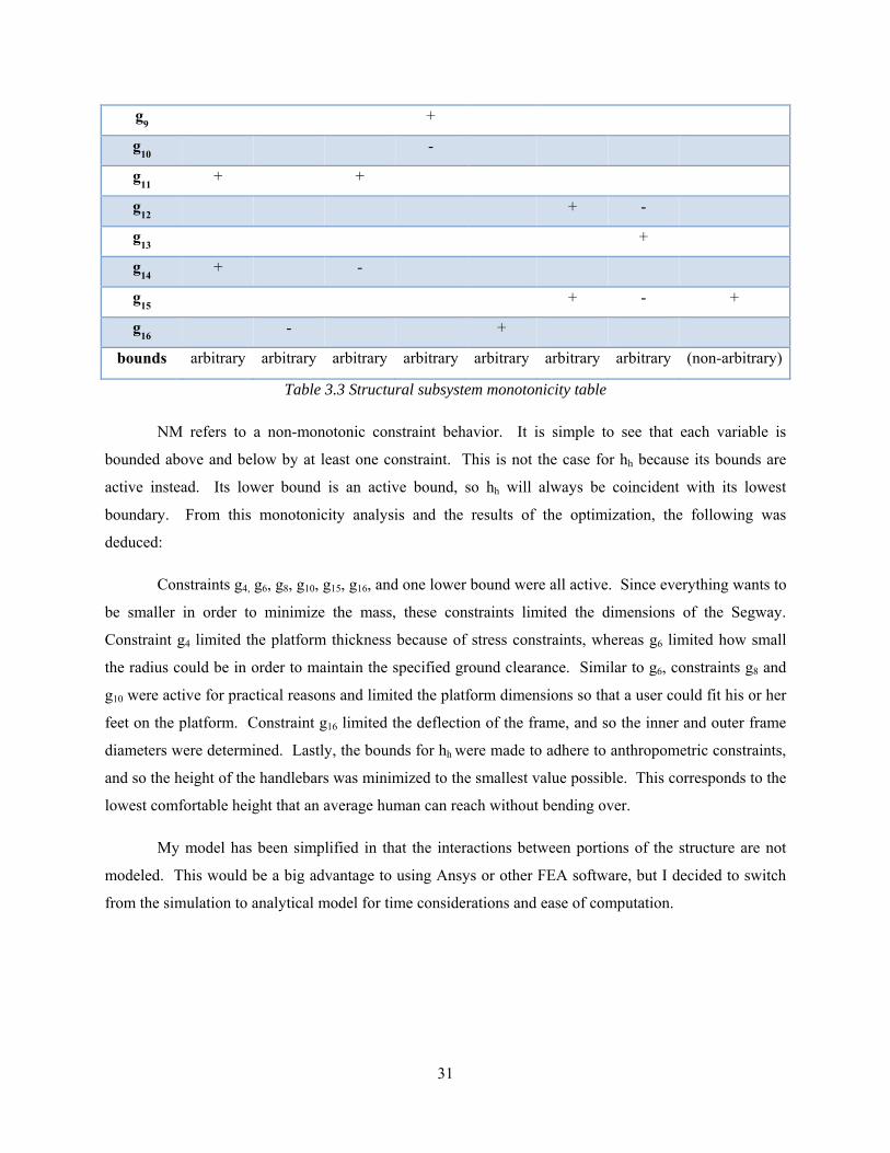
31

g9 +

g10 -

g11 + +

g12 + -

g13 +

g14 + -

g15 + - +

g16 - +

bounds arbitrary arbitrary arbitrary arbitrary arbitrary arbitrary arbitrary (non-arbitrary)

Table 3.3 Structural subsystem monotonicity table

NM refers to a non-monotonic constraint behavior. It is simple to see that each variable is

bounded above and below by at least one constraint. This is not the case for hh because its bounds are

active instead. Its lower bound is an active bound, so hh will always be coincident with its lowest

boundary. From this monotonicity analysis and the results of the optimization, the following was

deduced:

Constraints g4, g6, g8, g10, g15, g16, and one lower bound were all active. Since everything wants to

be smaller in order to minimize the mass, these constraints limited the dimensions of the Segway.

Constraint g4 limited the platform thickness because of stress constraints, whereas g6 limited how small

the radius could be in order to maintain the specified ground clearance. Similar to g6, constraints g8 and

g10 were active for practical reasons and limited the platform dimensions so that a user could fit his or her

feet on the platform. Constraint g16 limited the deflection of the frame, and so the inner and outer frame

diameters were determined. Lastly, the bounds for hh were made to adhere to anthropometric constraints,

and so the height of the handlebars was minimized to the smallest value possible. This corresponds to the

lowest comfortable height that an average human can reach without bending over.

My model has been simplified in that the interactions between portions of the structure are not

modeled. This would be a big advantage to using Ansys or other FEA software, but I decided to switch

from the simulation to analytical model for time considerations and ease of computation.

32

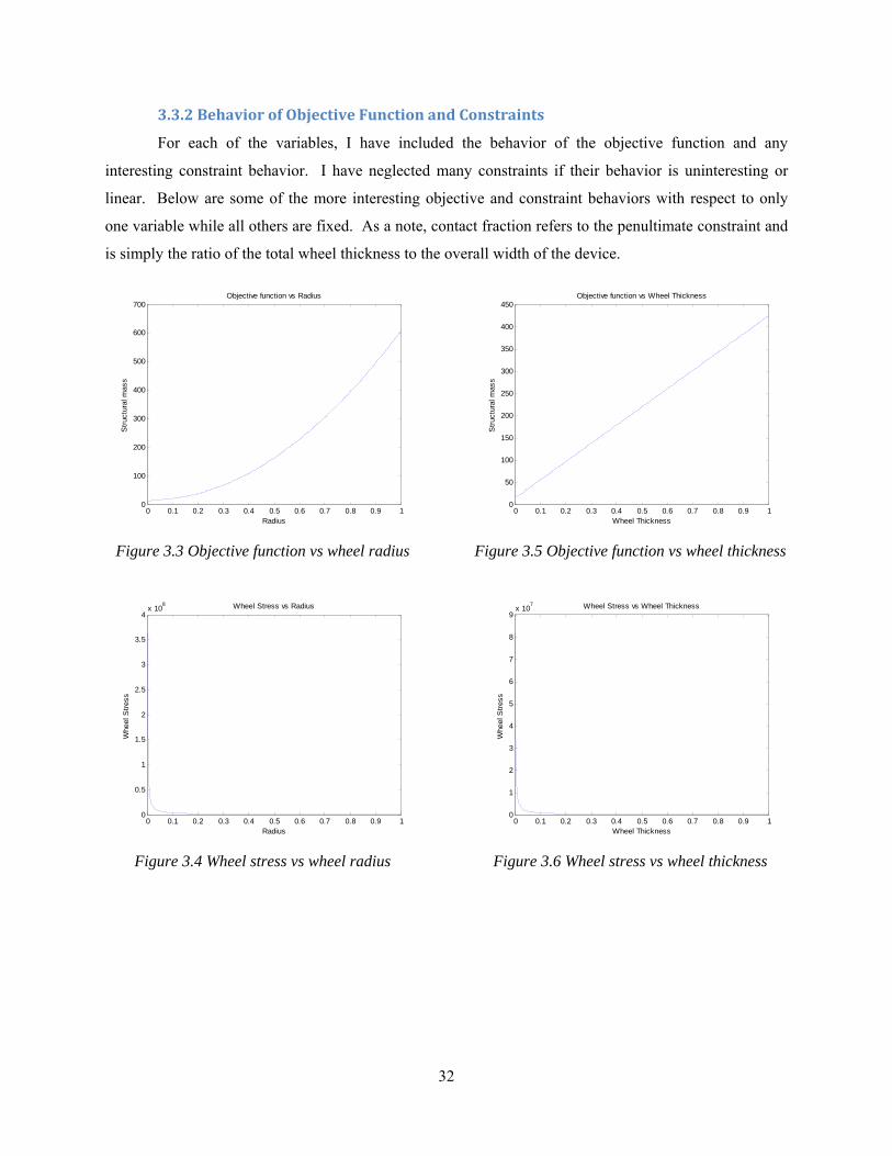
3.3.2 Behavior of Objective Function and Constraints

For each of the variables, I have included the behavior of the objective function and any

interesting constraint behavior. I have neglected many constraints if their behavior is uninteresting or

linear. Below are some of the more interesting objective and constraint behaviors with respect to only

one variable while all others are fixed. As a note, contact fraction refers to the penultimate constraint and

is simply the ratio of the total wheel thickness to the overall width of the device.

Figure 3.3 Objective function vs wheel radius

Figure 3.4 Wheel stress vs wheel radius

Figure 3.5 Objective function vs wheel thickness

Figure 3.6 Wheel stress vs wheel thickness

0 0.1 0.2 0.3 0.4 0.5 0.6 0.7 0.8 0.9 10

100

200

300

400

500

600

700Objective function vs Radius

Radius

Str

uctu

ral m

ass

0 0.1 0.2 0.3 0.4 0.5 0.6 0.7 0.8 0.9 10

0.5

1

1.5

2

2.5

3

3.5

4x 10

8 Wheel Stress vs Radius

Radius

Whe

el S

tres

s

0 0.1 0.2 0.3 0.4 0.5 0.6 0.7 0.8 0.9 10

50

100

150

200

250

300

350

400

450Objective function vs Wheel Thickness

Wheel Thickness

Str

uctu

ral m

ass

0 0.1 0.2 0.3 0.4 0.5 0.6 0.7 0.8 0.9 10

1

2

3

4

5

6

7

8

9x 10

7 Wheel Stress vs Wheel Thickness

Wheel Thickness

Whe

el S

tres

s

33

Figure 3.7 Contact fraction vs wheel thickness

Figure 3.8 Objective function vs platform

thickness

Figure 3.9 Objective function vs platform length

Figure 3.10 Platform stress vs platform length

Figure 3.11 Objective function vs platform width

Figure 3.12 Platform stress vs platform width

0 0.1 0.2 0.3 0.4 0.5 0.6 0.7 0.8 0.9 1-0.35

-0.3

-0.25

-0.2

-0.15

-0.1

-0.05

0

0.05

0.1Contact Fraction vs Wheel Thickness

Wheel Thickness

Con

tact

Fra

ctio

n

0 0.1 0.2 0.3 0.4 0.5 0.6 0.7 0.8 0.9 10

100

200

300

400

500

600

700

800Objective function vs Platform Thickness

Platform Thickness

Str

uctu

ral m

ass

0 0.1 0.2 0.3 0.4 0.5 0.6 0.7 0.8 0.9 120

22

24

26

28

30

32

34

36

38

40Objective function vs Platform Length

Platform Length

Str

uctu

ral m

ass

0 0.1 0.2 0.3 0.4 0.5 0.6 0.7 0.8 0.9 10

0.5

1

1.5

2

2.5x 10

8 Platform Stress vs Platform Length

Platform Length

Pla

tfor

m S

tres

s

0 0.1 0.2 0.3 0.4 0.5 0.6 0.7 0.8 0.9 120

22

24

26

28

30

32

34Objective function vs Platform Width

Platform Width

Str

uctu

ral m

ass

0 0.1 0.2 0.3 0.4 0.5 0.6 0.7 0.8 0.9 10

0.5

1

1.5

2

2.5x 10

8 Platform Stress vs Platform Width

Platform Width

Pla

tfor

m S

tres

s

34

Figure 3.13 Contact fraction vs platform width

Figure 3.14 Objective function vs Outer frame

diameter

Figure 3.15 Pipe stress vs outer frame diameter

Figure 3.16 Frame deflection vs outer diameter

Figure 3.17 Objective function vs frame

diameter

Figure 3.18 Pipe stress vs frame diameter

0 0.1 0.2 0.3 0.4 0.5 0.6 0.7 0.8 0.9 1-0.45

-0.4

-0.35

-0.3

-0.25

-0.2

-0.15

-0.1

-0.05

0

0.05Contact Fraction vs Platform Width

Platform Width

Con

tact

Fra

ctio

n

0 0.1 0.2 0.3 0.4 0.5 0.6 0.7 0.8 0.9 1-2000

-1500

-1000

-500

0

500Objective function vs Outer Frame Diameter

Outer Frame Diameter

Str

uctu

ral m

ass

0 0.1 0.2 0.3 0.4 0.5 0.6 0.7 0.8 0.9 1-2

-1.5

-1

-0.5

0

0.5

1

1.5

2

2.5x 10

8 Pipe Stress vs Outer Frame Diameter

Outer Frame Diameter

Pip

e S

tres

s

0 0.1 0.2 0.3 0.4 0.5 0.6 0.7 0.8 0.9 1-0.02

-0.015

-0.01

-0.005

0

0.005

0.01

0.015

0.02

0.025Frame Deflection vs Outer Diameter

Outer Diameter

Fra

me

Def

lect

ion

0 0.1 0.2 0.3 0.4 0.5 0.6 0.7 0.8 0.9 10

500

1000

1500

2000

2500Objective function vs Inner Frame Diameter

Inner Frame Diameter

Str

uctu

ral m

ass

0 0.1 0.2 0.3 0.4 0.5 0.6 0.7 0.8 0.9 1-8

-7

-6

-5

-4

-3

-2

-1

0

1x 10

8 Pipe Stress vs Inner Frame Diameter

Inner Frame Diameter

Pip

e S

tres

s

35

Figure 3.19 Frame deflection vs inner diameter

Figure 3.20 Objective function handlebar height

Figure 3.21 Pipe stress vs handlebar height

Figure 3.22 Frame deflection vs handlebar

height

A few notes about the plots above: In some of the frame diameter plots, there is a discontinuous

region. This is caused by one of the diameters crossing the other one. In effect, the outer and inner

diameters switch roles. Physically, this cannot happen, however when all other variables are fixed and

the behavior of the objective or constraints is observed with respect to only one variable, mathematical

nuances like this appear. This is also evident in the obviously non-monotonic behavior of the platform

width and length plots when looking at their respective effects on the platform stress. This dip in the

stress can be explained by the values of lp and wp approaching each other. When the platform is a square,

the stress is the lowest, which makes intuitive sense.

0 0.1 0.2 0.3 0.4 0.5 0.6 0.7 0.8 0.9 1-0.07

-0.06

-0.05

-0.04

-0.03

-0.02

-0.01

0

0.01Frame Deflection vs Inner Diameter

Inner Diameter

Fra

me

Def

lect

ion

0 0.1 0.2 0.3 0.4 0.5 0.6 0.7 0.8 0.9 122

23

24

25

26

27

28

29Objective function vs Handlebar Height

Handlebar Height

Str

uctu

ral m

ass

0 0.1 0.2 0.3 0.4 0.5 0.6 0.7 0.8 0.9 10

1

2

3

4

5

6

7x 10

6 Pipe Stress vs Handlebar Height

Handlebar Height

Pip

e S

tres

s

0 0.1 0.2 0.3 0.4 0.5 0.6 0.7 0.8 0.9 10

1

2

3

4

5

6x 10

-4 Frame Deflection vs Handlebar Height

Handlebar Height

Fra

me

Def

lect

ion

36

3.4 Optimization Study

I used the fmincon functionality in MATLAB, which is an implementation of the sequential

quadratic programming algorithm, for this optimization and found it to be reasonably well-suited for the

problem. I did encounter some bugs, but I think overall, fmincon worked to optimize for the minimum

mass. I found the optimum to be the Carbon Fiber with the following dimensions

r t hp lp wp dfi dfo hh

.1516 .0347 .0032 .45 .6245 .0918 .0963 .951

Table 3.4 Optimum for carbon fiber

The following plot shows the convergence rate of my model when fmincon was used. This

convergence is very quick and smooth which indicates that perhaps the model was a simple one for the

algorithm to solve.

Figure 3.23 Objective function vs. iteration

Constraints 4,6,8,10,15 and 16 were active. The final mass was 11.58kg and the final Cost was

$382.14. All of this falls within the constraints, however I don’t think it is the best option.

0 1 2 3 4 5 6 725

30

35

40

45

50

55

60

65

70

Iteration

Fun

ction va

lue

Current Function Value: 28.5198

37

3.5 Parametric Study

After doing parametric studies for the material and the load, I think that the best material is

Aluminum 6061. Here are the numerical results of the parametric study with respect to material.

r t hp lp wp dfi dfo hh Mass Cost

k = 1 0.1563 0.0344 0.0126 0.45 0.6186 0.0859 0.0924 0.951 77.1 267.9995

k = 2 0.1539 0.032 0.0078 0.45 0.5765 0 0.0643 0.951 77.5778 402.0406

k = 3 0.1542 0.0346 0.0084 0.45 0.6229 0.0899 0.0953 0.951 64.95 450

k = 4 0.1555 0.035 0.011 0.45 0.63 0.0838 0.1 0.951 28.8208 126.8115

k = 5 0.1541 0.035 0.0081 0.45 0.63 0.0846 0.1 0.951 27.103 432.7795

k = 6 0.1516 0.0347 0.0032 0.45 0.6245 0.0918 0.0963 0.951 11.5801 382.1446

Table 3.5 Numerical results of the parametric study with respect to material

The third-lowest mass was the cheapest, by far, and I think it is the best choice given the

constraints and parameters.

Figure 3.24 System mass vs load

0

20

40

60

80

100

0 500000 1000000 1500000 2000000

System M

ass

Load

System mass vs Load

38

Load r t hp lp wp dfi dfo hh Mass Cost

40 0.1502 0.035 0.0003 0.45 0.63 0.0838 0.1 0.951 19.677 86.5788

400 0.1506 0.035 0.0011 0.45 0.63 0.0838 0.1 0.951 20.3215 89.4147

4000 0.1517 0.035 0.0035 0.45 0.63 0.0838 0.1 0.951 22.3608 98.3877

400000 0.1674 0.035 0.0349 0.45 0.63 0.0838 0.1 0.951 49.3601 217.1843

1000000 0.1776 0.035 0.0551 0.45 0.63 0.0838 0.1 0.951 66.9487 294.5742

2000000 0.1889 0.0337 0.0779 0.45 0.6066 0 0.0844 0.951 92.1844 405.6112

Table 3.6 Parametric study on different materials and corresponding optimum

This figure represents the mass as a function of the load. It gets incredibly high for this material

(Al 6061). The other materials had similar plots of system mass versus load.

I also performed a parametric study on cost and found those very boring since they were

infeasible until the price listed in the optimal table above, after which, they were constant.

3.6 Discussion of Results

From the above results, one may see many trends. For instance, the dimensions of the Segway

system actually don’t change much even when very different materials are chosen. This is probably

because my model is very tightly constrained and many of the constraints are dimensional for ergonomic

or tolerance considerations. It is these constraints that are active, although a stress constraint is also

active, which explains the minor differences in the designs. Also, given a very wide range of initial

starting points for the model, fmincon seemed to always find the same solution. This indicates that the

optimum found may be global. This is not a terribly surprising result since my model was fairly simple

and consisted of mostly monotonic linear and quadratic functions. Since fmincon is an implementation of

a gradient-based algorithm, simple monotonic functions are well-suited to this solver. In my parametric

studies, it seems obvious that mass and cost will increase with respect to increased load. One can

intuitively think that with a larger load on the platform, the thickness of the platform will need to be

greater. This is seen in the study and reflected in the objective.

The final design of the optimized structural system can be seen in the following images:

39

Figures 3.25-27 Structural subsystem optimized design model, views 1-3

40

3.7 System Tradeoffs

The structural system did not actually have trade-offs in the end since we used a sequential

approach for the entire system and since my subsystem did not depend on any of the others. The overall

objective was actually reduced in the system optimization since the fmincon options were changed to very

small step sizes. For this reason, the system optimization found a slightly better optimum that my

subsystem did not find since the step size was large enough for it to skip over. Minimizing the mass

actually helps the other subsystems for the most part. This can be seen in the overall system optimization

at the end of this report. A decreased mass will actually increase the transmissibility, which is the

subsystem objective for the dynamics and vibrations subsystem. With this as a constraint, it is possible

that my subsystem objective may not be the system objective. As it turned out, I could optimize the

structure while not interfering with the transmissibility since the masses of the user and the electrical

system were enough to actually decrease the transmissibility from the value obtained in the subsystem

level.

41

4. Electrical Subsystem

4.1. Introduction

The electrical subsystem comprises of the battery and two electrical motors, one for each wheel.

The objective of this subsystem is to optimize the motor and the battery sizes in order to maximize the

travelling range of the Segway transporter. A base capacity of 2hp each has been chosen for the motor

based upon commercially available models while a battery of capacity 6Ah and 72 Volts has been chosen

as the base model. These motors and battery packs were scaled appropriately in order to optimize the

electrical subsystem. In order to do so, scaling factors were introduced for the motor size, battery voltage

and battery capacity. These scaling factors were optimized in order to reach an optimum solution.

The model used for the electrical subsystem comes from an existing SIMULINK model of an

automobile which has been suitably modified [6].



The main objective of this subsystem is to maximize the distance covered by the Segway in a

single charge while catering to the constraints on minimum top speed, total cost, weight, operating

efficiency of motor, maximum allowable current through the circuit and the minimum threshold state of

charge of the battery that can be reached.

max, ,

Distance

This can be written as a minimization problem as follows:

min,, ,

Distance

Thus, minimizing the negative of the distance or the range of the Segway is the same as

maximizing the distance. Maximizing the range has been taken as an objective of this sub-system since

the entire electrical system is based on the range and speed required only. The range dictates the voltage

42

and capacity of the battery pack to be used while the speed plays a major role in deciding the motor

sizing.

4.2.2 Constraints

An upper bound has been set on the total weight of the electrical system since an absence of this

constraint will result in indefinite sizing of the battery in order to achieve maximum range. The constraint

on the minimum top speed has been set in order to size the motor appropriately and hence, to clearly

define the feasible domain. Another constraint on the cost of motor ensures that the motor cost does not

go beyond the upper bound on the cost. The next constraint is on the motor efficiency in order to verify

that the motor is operating at its efficient region. A constraint binding the maximum current through the

circuit has also been set.

g1: w – 20 ≤ 0

g2: 20 – v ≤ 0

g3: m_cost – 1000 ≤ 0

g4: 0.70 – eta_m ≤ 0

g5: Imax – 60 ≤ 0

The following Constraints are validated implicitly in the SIMULINK model:

g6: 0.2 – soc ≤ 0

g7: P_supplied – ((Voc / 2)2/Rint) ≤ 0

4.2.3 Governing Equations

1. ess_voc = f1 (SOC) … 4.1

2. ess_dis =f2 (SOC) … 4.2

3. ess_chg =f3 (SOC) … 4.3

4. I

VOC VOC P R

R for VOC 4P R 0

VOCR

VOC 4P R 0 … 4.4

5. Vbat = VOC – (Ibat * Rint) … 4.5

6.

… 4.6

43

7. _ _ _

_ _ … 4.7

8. wm = m_specific X Pm … 4.8

9. N_tire = v/2ΠRw … 4.9

10. N_motor = N_tire * TR … 4.10

11. m_cost = f5 (sfm) … 4.11

4.2.4 Model Summary

Design Variables

S.No. Symbol Description Unit

1 sfm Scaling factor for motor -

2 sbv Scaling factor for battery voltage -

3 sba Scaling factor for battery capacity -

Table 4.1 Electrical subsystem design variables

Design Parameters

S.No. Symbol Description Assumed Value

1 vmax Maximum speed required 20 km/h

2 TR Transmission ratio 20

3 Rw Tire Radius 0.20 m

4 torque Torque requirement from user 6 Nm

5 Af Frontal Area of cross-section 0.7 m2

6 Mv Total mass (Segway + Payload) 150 kg

7 ess_init_soc Initial SOC 0.9

Table 4.2 Electrical subsystem parameters

4.2.5 Coding for Numerical Processing:

From the equation

Pbat = Voc*Ibat – Ibat2Rint … 4.12

We get

44

Ibat VOC VOC 4P R

2R… 4.13

In cases whenVOC 4P R 0, attempt to take the square root of a negative quantity will

result in complex numbers. This situation arises typically when the power required is higher than the

power available in the battery. Hence, in such situations, I = Voc/ 2Rint is used. This is also the

maximum current that the battery can provide. Similarly, in order to avoid division by zero and also to

have non-zero values of the scaling factors, the lower bounds of all the scaling factors have been set as

0.1.

4.3 Model Analysis

4.3.1 Monotonicity Analysis:

The objective function cannot be analytically written in terms of the design variables in order to

perform monotonicity analysis as done conventionally. The objective function is an indirect function of

all the design variables and hence, an intuitive and reason based monotonicity analysis has only been

provided.

Objective

min,, ,

, ,

Subject To

g1: w – 20 ≤ 0

w = wm + wb

wm = 11.0474*sfm

wb = 3.99168*sbv*sba

Hence,

g1: (11.0474*sfm + 3.99168*sbv*sba) – 20 ≤ 0

g2: 20 – v ≤ 0

The velocity is a function of the scaling factor of the motor sfm and hence,

45

g2: 20 – f1 (sfm) ≤ 0

g3: m_cost – 1000 ≤ 0

m_cost = 289.677*sfm + 223.42

Hence,

g3: (289.677*sfm + 223.42) – 1000 ≤ 0

g4: 0.70 – eta_m ≤ 0

g5: Imax – 60 ≤ 0

Imax = f2 (l/Voc) and hence, Imax = f2 (l/sbv)

Hence,

g5: f2 (l/sbv) – 60 ≤ 0

g6: 0.2 – soc ≤ 0

soc = f3 (sba)

Hence,

g6: 0.2 – f3 (sba) ≤ 0

The role of sfm on the objective function as well as the constraints is difficult to explain since

there are many factors which might result in either an increase or a decrease of the objective function or

the constraint by a corresponding change in sfm. This is because, an increase in sfm might push the motor

to operate in a more or a less efficient region of operation and hence, the distance might increase or

decrease. Increasing sbv and sba will result in an increase in the distance due to higher battery life and

hence, this will lead to a decrease in the objective function which is the negative of the distance covered.

Hence, mathematically

min,, ,

, ,

Subject to

1 , , ; 2 ; 3 ; 4 ; 5 ; 6

46

The monotonicity with respect to sbv and sba can be interpreted as follows. An increase in both

voltage as well as battery capacity will result in a greater range and hence, the value of the objective

function increases as sbv and sba increase. On the other hand, the constraint g5 decreases as sbv increases

and g6 decreases as sba increases. Hence, g5 and g6 can be considered active constraints. It is very

difficult to draw any conclusions about constraint activity with respect to sfm as it’s a highly complex

function.

4.3.2 WellBoundedness:

It is not possible to talk explicitly about well boundedness in this problem since the relationships

are not linear. However, both lower and upper bounds have been assigned to the design variables and

hence, we can consider the problem to be well bounded.

S. No. Variable Lower bound Upper bound

1 sfm 0.1 5

2 sbv 0.1 5

3 sba 0.1 5

Table 4.3 Bounds of the design variables


4.4.1 Optimizer Settings

S.No. Option Setting

1 Algorithm active-set

2 Display iter-detailed

3 DiffMinChange 1e-10

4 TolX 1e-8

5 TolCon 1e-8

6 TolFun 1e-8

7 PlotFcns @optimplotx

8 PlotFcns @optimplotfval

Table 4.4 Optimizer settings

47

4.4.2 Results and Possible Local Minima

In order to compute the true range of the Segway, the simulation should be run for a minimum of

about 3000 to 4000 seconds for each iteration of the optimizer. But, this results in “Memory Allocation

Errors” when run from the function. Hence, I have scaled down the problem in order to run it for ten

seconds alone for each iteration. After obtaining the optimum values of the scaling factors, I have

computed the true range of the Segway with a fully charged battery.

S.No. Initial Point

[sfm,sbv,sba] sfm sbv sba fval

wm

kg

wb

kg

m_cost

$

True Range

km

1 [0.9, 3, 1] 1.0365 2.9233 0.7327 -55.6436 11.45 8.51 523.7 18.34

2 [5, 5, 5] 1.2287 1.2688 1.2688 -55.6550 13.57 6.43 579.4 24.097

3 [1, 2, 1] 0.9991 2 1 -55.650 11.04 7.98 512.8 23.303

Table 4.5 Optimization results

The above set of values obtained for different starting points indicates that there no single global

minima, but, a set of possible local minima. The second and third sets of values for the design variables

are pretty different from each other. In spite of this, both the cases have almost the same range. This can

be attributed to the fact that the second case has moderate values of both the battery voltage as well as the

capacity while the third case clearly has a lesser capacity but a greater voltage which reduces the current

flow and hence, the SOC of the battery decreases much slower when compared to a battery with sbv=1

and sba=1.

Taking a specific price of $730 / kWh [8] for the batteries, the battery costs $253.84 for the second

case while it costs $315.36 for the third. Computing the overall cost of the electrical system, the second

one comes at a cost of $833.24 while the third one costs $828.16. Hence, the specifications of the second

one are better for a commercial Segway since a $5 extra cost will give almost a kilometer of extra range.


A parametric study of the change of the optimum values of the design variable upon changing the

maximum speed required was conducted and the following results were obtained. The starting point was

fixed at [1, 2, 1].

48

vmax (km/h) sfm sbv sba

22 1.1237 1.9794 0.9589

20 0.991 2 1

18 0.9998 2 1

16 0.9938 2 1

14 1 2 1

Table 4.6 Parametric study: required maximum speed

Figure 4.1 Parametric study: required maximum speed

The trends observed in the above plot clearly shows that the motor sizing is the alone affected by

changes in the top speed required since the battery voltage and capacity are more associated with the

range of the Segway rather than the top speed. The up and down variation of the scaling factor of the

motor with increase in top speed can be attributed to the change in the efficient operating region of the

motor with increase in velocity and hence, the load.

0

0.5

1

1.5

2

2.5

0.990.9910.9920.9930.9940.9950.9960.9970.9980.999

11.001

12 14 16 18 20 22 24

sfm

vmax (km/h)

Parametric Study

sfm

sbv

sba

49


The results indicate the existence of several local minima. This can be accounted to the fact that

several different combinations of battery voltage and capacity can result in the same range of the segway

and hence, the starting point plays a big role in the optimum point reached. The monotonicity with respect

to the battery is not predictable since the objective function, the range, is slightly affected by the operating

efficiency of the battery and for the same torque requirement, the efficiency of the motor may be more or

less depending on the operating speed of the motor. Since the model was computationally intense and

required a long time and memory for simulation, the problem was scaled down to be run for ten seconds.

But, this resulted in reduced average velocity since the PID controller used in the electrical subsystem

required some minimum settling time for the velocity to settle down and hence, the constraint was slightly

relaxed in the scaled down version. However, in the complete test for the range upon reaching the

optimum showed that the average velocity was equal to the required velocity.

4.7 System Tradeoffs

(1) The electrical subsystem has been designed for assumed values of various parameters like the

total mass, cross-sectional area, torque requirement, tire radius etc. The values of these

parameters might change based on the design variables of other subsystems and hence, these

parameters and also the design variables need to be reworked and changed accordingly in

order to optimize the entire system.

(2) Conflicts regarding the cost distribution between sub-systems may result in the need for

changes in the design variables in order to accommodate for the changes in cost allocation.

(3) Space and packaging constraints if considered, might result in tradeoff’s between the

available space and the size of the battery and motor.

(4) The range of the segway was made a constraint in the system level while the subsystem mass

was made the objective function. Hence, the required range to be achieved in ten seconds was

placed as a constraint on the distance. However, the optimum points found did not result in

the same total range expected when they were plugged into the stand alone model and tested

for a period of 3600 secs since the battery performance is not linear and hence, the

performance for 10 secs cannot be assumed to be equal to that for the entire time span.

50

5. Vibrations Subsystem

5.1 Introduction

This subsystem, passenger comfort and vibrations, aims to minimize the acceleration felt by the

rider for a given road excitation. Noticing the fact that currently there is no known suspension system for

the segway, designing such a suspension for the segway to reduce abrupt and unwanted acceleration felt

by the rider could add additional market value to the segway. The subsystem deals with the interactions

between the ground and the segway wheels, as well as the performance of the newly designed suspension

system, which is greatly inspired by those that are already widely used in automobiles and is to be put in

between the wheels and the segway.


5.2.1 Description of the System

The model used for the subsystem comes from existing linear models developed for an

automobile performance and will be modified to accommodate the Segway [9]. The simplified system

diagram is shown below. It takes into account elastic and damping effect added to the system by the

interactions between the tires and the ground, expressed in terms of equivalent spring constant (k_T) and

damping coefficient (c_T). The two tires are simply modeled as a mass (m_T) since that’s the only thing

that would influence the acceleration felt by the rider. Also, an imaginary suspension system, composed

of a spring (k_S) and a damper (c_S), is inserted in between the wheels and the platform of the segway.

All the other parts of the segway, including the platform (chassis, motor, microchips), the standing control

shaft and the handle bar, as well as the rider are modeled as one single mass (m_S). This parameter is so

designed to simplify the analysis and avoid potential conflicts with other subsystem when integrating

them in the future.

A sinusoidal ground excitation is used since it is the most common form of external disturbance.

It is expressed in terms of displacement, z_G. See appendix for detailed derivation of governing equations

of the system

51



The minimization of the acceleration felt by the segway rider is decided to be the main objective

since it directly affects the comfort and ride quality. To apply the concept of transmissibility, which is

simply defined as the ratio of output to input, the objective function is so created to minimize the ratio of

the acceleration felt by human to the acceleration due to ground excitation. That is,

minzSzG

Since both accelerations zS (segway rider) and zG (ground) are varying time series data,

a statistical measure of the magnitude of a varying quantity, the root mean square (RMS) is calculated for

both of them. That’s what the notation | | in the above equation means. The value of the objective

function is considered reasonable if it is less than one, which means that the acceleration felt by the rider

is smaller than that generated by ground excitation.

5.2.3 Constraints

For the spring constants (k_S, k_T) and the damping coefficients (c_S,c_T), a lower limit was

established to prevent the springs and the dampers to be too soft for the system to work properly. For

instance, imagine a spring being compressed to its bottom height all the time, it brings no effect to the

whole system. On the other hand, an upper limit was also needed for those four parameters to prevent

them to be too stiff. If that is the case, then the suspension system can be treated as a rigid connection

between the tires and the segway platform, which will lose its suspension functionality. There were also

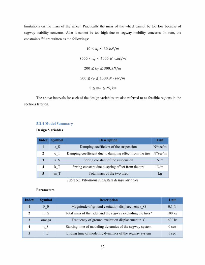
52

limitations on the mass of the wheel. Practically the mass of the wheel cannot be too low because of

segway stability concerns. Also it cannot be too high due to segway mobility concerns. In sum, the

constraints [10] are written as the followings:

10 30, /

3000 5000, · /

200 300, /

500 1500, · /

5 25,

The above intervals for each of the design variables are also referred to as feasible regions in the

sections later on.

5.2.4 Model Summary

Design Variables

Index Symbol Description Unit

1 c_S Damping coefficient of the suspension N*sec/m

2 c_T Damping coefficient due to damping effect from the tire N*sec/m

3 k_S Spring constant of the suspension N/m

4 k_T Spring constant due to spring effect from the tire N/m

5 m_T Total mass of the two tires kg

Table 5.1 Vibrations subsystem design variables

Parameters


1 F_0 Magnitude of ground excitation displacement z_G 0.1 N

2 m_S Total mass of the rider and the segway excluding the tires* 100 kg

3 omega Frequency of ground excitation displacement z_G 60 Hz

4 t_S Starting time of modeling dynamics of the segway system 0 sec

5 t_E Ending time of modeling dynamics of the segway system 5 sec

53

6 V_S_S Starting value of the vertical velocity of the segway rider 0 m/sec

7 V_T_S Starting value of the vertical velocity of the tires 0 m/sec

8 z_S_S Starting value of vertical displacement felt by the segway rider 0 m

9 z_T_S Starting value of vertical displacement of the tires 0 m

*Temporary value. The value should come from the optimized result of the structural subsystem.

Table 5.2 Vibrations subsystem parameters

Constant


1 g Gravity 9.8 m/sec2

Table 5.3 Vibrations subsystem constant

Summary

Objective Function

Transmissibility will be used later on to refers to the objective function of the vibrations

subsystem

Subject to:

Upper Bound Lower Bound

: , g : kS 10,000 0

: g : cS 3000 0

: , g : kT 200,000 0

: g : cT 500 0

: g : mT 5 0

Table 5.4 Vibrations subsystem constraints

There are zero equality constraints and ten inequality constraints. Degrees of freedom cannot be

determined at this point due to the fact that number of active constraints cannot be determined. The reason

is that there is no explicit expression for the objective function and monotonicity of each design variables

54

is not clear. However the problem is well bounded since there are both upper and lower bounds for each

of the design variables.

5.3 Model Analysis

5.3.1 Monotonicity Analysis

Due to the complexity of the objective function, monotonicity analysis cannot be done in a

conventional manner. Rather, some analysis can still be done to explore the relationship between the

objective function and the design variables. The objective function (transmissibility) values were plotted

with only one design variable changing and all the other design variables fixed at the values of their

starting points. The results are shown below:

Figure 5.2 Transmissibility vs c_S Figure 5.3 Transmissibility vs c_T

Figure 5.4 Transmissibility vs k_S Figure 5.5 Transmissibility vs k_T


55

To add physical meaning to the plots above, first notice that the influence on the objective

function caused by suspension system design variables (k_S and c_S) was just the opposite of that by tire

dynamics design variables (k_T and c_T). This was verified if simply analyzing the force balance for the

tires. Forces generated by those two sets of variables got canceled due to their opposite directions.

Secondly, the objective function decreased almost monotonically with the mass of the tires. A low-mass

tire is desired so that only small amount of inertia force can be transmitted to the segway rider, reducing

the acceleration felt by the rider.

In addition, all the plots above showed a lot of noise in this minimization problem. This noise can

easily cause some optimization algorithm to get stuck in some local minimum, failing to find the global

minimum.

5.3.2 Constraints Activity

This was done by changing the constraint and checking whether or not the values of the objective

function and the design variables also changes.

Nomad Optimization Software was implemented in this analysis. MATLAB optimization

algorithm fmincon was not used here since it got stuck easily in the vicinity of the starting point as was

explained in the monotonicity analysis session.

The optimization results obtained by Nomad are shown below and it will be used as comparison

basis for checking constraint activity:

Before After

fval 0.5623 0.3508

k_S 20000 29940

c_S 4000 3000

k_T 250000 200592

c_T 1000 1496

m_T 5 5.625

Table 5.5 Nomad optimization results

56

Summary of constraint activety

Constraint Number Activity

1 Active (strong)*

2 Inactive

3 Inactive

4 Active (strong)

5 Active (weak)*

6 Active (weak)

7 Active (strong)

8 Active (strong)

9 Active (weak)

10 Active (strong)

* Strong/weak activity indicates significance of changes in objective function or optimum solution. Table 5.6 Summary of constraint activity\

Link monotonicity analysis (non-conventional approach in this project) to the activity analysis:

Mathematically:

, , , ,

Subject to:

; ; ; ; ; ; ; ; ;

It can be found that (1) if function value goes down as a constraint goes to zero, the constraint is

always active (strong). This can be verified for constraints g1, g4, g7, g8, g10. And this resembles very

much to monotonicity principle 1. (2) On the other hand, if the function value goes up as a constraint goes

to zero, the constraint can be active (weak) OR inactive. This can be verified for constraints g5, g6, g9

OR g2, g3. The non-linear nature of the minimization problem might cause this. The following pictures

demonstrate the above two points graphically.

57




Inactive constraint

Active constraint (weak)

Active constraint (strong)

58

5.3.3 Wellboundedness

The well-boundedness cannot be verified since the monotonicity of the minimization problem is

still not clear. However, the problem can be said to be well-bounded since there are both lower and upper

bounds for each of the design variables.


5.4.1 Approach 1: Changing Starting Points

Here a method of finding starting points was explored so that hopefully better solutions can be

found. Plot objective function with one changing design variable changing and others fixed using the

starting points 20000,4000,250000,500,15 :




59

Minimum point of function value vs. one changing design variable only

Collect minimum points from each of the graphs above and form a new set of starting points.

Repeat the procedure, plot objective function with one changing design variable changing and others

fixed using the new starting points x2, collect minimum points, and so on so forth. Four different sets of

starting points are:

x1 x2 x3 x4

k_S 20000 30000 23240 17400

c_S 4000 3000 3000 3000

k_T 250000 300000 200000 200000

c_T 500 1500 1500 1480

m_T 15 5 5 5.4

Table 5.7 Different sets of starting points

Nomad was used to check how good the starting points are:

x1 x2 x3 x4

fval 0.3508 0.3482 0.3481 0.3480

k_S 29940 28342 17608 29980

c_S 3000 3000 3000 3000

k_T 200592 200032 200000 200000

c_T 1496 1469.5 1500 1499.75

m_T 5.625 5 5 5.3883

Table 5.8 Nomad: optimization results for different sets of starting points

Nomad searched a greater area of feasible region than fmincon and the starting points did help the

objective function values get improved values. Also function convergence was improved:

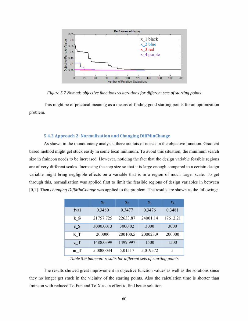
60

Figure 5.7 Nomad: objective functions vs iterations for different sets of starting points

This might be of practical meaning as a means of finding good starting points for an optimization

problem.

5.4.2 Approach 2: Normalization and Changing DiffMinChange

As shown in the monotonicity analysis, there are lots of noises in the objective function. Gradient

based method might get stuck easily in some local minimum. To avoid this situation, the minimum search

size in fmincon needs to be increased. However, noticing the fact that the design variable feasible regions

are of very different scales. Increasing the step size so that it is large enough compared to a certain design

variable might bring negligible effects on a variable that is in a region of much larger scale. To get

through this, normalization was applied first to limit the feasible regions of design variables in between

[0,1]. Then changing DiffMinChange was applied to the problem. The results are shown as the following:

x1 x2 x3 x4

fval 0.3480 0.3477 0.3476 0.3481

k_S 21757.725 22633.87 24001.14 17612.21

c_S 3000.0013 3000.02 3000 3000

k_T 200000 200100.5 200023.9 200000

c_T 1488.0399 1499.997 1500 1500

m_T 5.0000034 5.01517 5.019572 5

Table 5.9 fmincon: results for different sets of starting points

The results showed great improvement in objective function values as well as the solutions since

they no longer get stuck in the vicinity of the starting points. Also the calculation time is shorter than

fmincon with reduced TolFun and TolX as an effort to find better solution.

x_1 black x_2 blue x_3 red x_4 purple

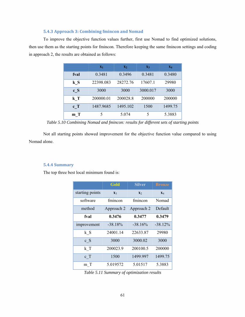
61

5.4.3 Approach 3: Combining fmincon and Nomad

To improve the objective function values further, first use Nomad to find optimized solutions,

then use them as the starting points for fmincon. Therefore keeping the same fmincon settings and coding

in approach 2, the results are obtained as follows:

x1 x2 x3 x4

fval 0.3481 0.3496 0.3481 0.3480

k_S 22398.083 28272.76 17607.1 29980

c_S 3000 3000 3000.017 3000

k_T 200000.01 200028.8 200000 200000

c_T 1487.9685 1495.102 1500 1499.75

m_T 5 5.074 5 5.3883

Table 5.10 Combining Nomad and fmincon: results for different sets of starting points

Not all starting points showed improvement for the objective function value compared to using

Nomad alone.

5.4.4 Summary

The top three best local minimum found is:

Gold Silver Bronze

starting points x3 x2 x4

software fmincon fmincon Nomad

method Approach 2 Approach 2 Default

fval 0.3476 0.3477 0.3479

improvement -38.18% -38.16% -38.12%

k_S 24001.14 22633.87 29980

c_S 3000 3000.02 3000

k_T 200023.9 200100.5 200000

c_T 1500 1499.997 1499.75

m_T 5.019572 5.01517 5.3883

Table 5.11 Summary of optimization results

62

Therefore fmincon with normalization and increased search step size turned out to be the best for

the optimization of the subsystem. It was also noticed that non-gradient based method Nomad showed an

uncompromising performance to the problem with only its default settings.

Constraints 4, 7, 8, 10 are active, as indicated as strong activity in the monotonicity analysis.

Therefore the corresponding design variables c_S, k_T, c_T, m_T are boundary solutions. Constraints 1

and 6 are not active since the value of k_S turned out to be an interior solution. Monotonicity principle 1

made a very good prediction of the constraint activity for such a nonlinear problem. The final solutions

are local optimum, especially with respect to design variable k_S. This is because high non-linearity of

the objective function with k_S changing, as indicated below:

Figure 5.4 Transmissibility vs k_S

Numerical stability was good using Nomad and fmincon, with less than one percent of change in

the objective function value for different sets of starting points.

63


5.5.1 Transmissibility vs F_0

Figure 5.8 Transmissibility vs F_0

F_0 is the magnitude of ground excitation displacement z_G. The objective function displays a

high non-linearity and noisy behavior with respect to F_0. Although it increases with F_0, the objective is

insensitive to this parameter since the change of its value is not significant. Since the objective is defined

as the ratio of accelerations, it cannot quantify the change in the magnitude of acceleration felt by the

segway rider when ground excitation gets worse. This parametric study indicates a necessity to modify

the objective function to measure the change in the magnitude of acceleration.

5.5.2 Transmissibility vs m_S

Figure 5.9 Transmissibility vs m_S

64

m_S is the total mass of the rider and the segway excluding the tires. The objective decreases as

the m_S increases. This is intuitively understandable since the transmissibility will improve if there is

more inertia in the system to resist the disturbance caused by external force. Also notice that the objective

function is very sensitive to this parameter. The value of m_S in the current system is set to be 100kg

based on the averaged mass of the rider and the segway. This parametric study inspired some future work

to introduce a certain range of masses of riders into the model and redesign the objective function to

incorporate that.


In the final result the objective reached a value of about 0.34 from the initial value of 0.51. This

means that the segway rider felt one third of the ground excitation acceleration than initially the half

acceleration, which is quite an improvement. First it was noticed that the mass of the segway wheels

reached its lower bound. This is consistent with the monotonicity analysis and it makes physical sense

since minimum inertia force from the wheels was desired to be transmitted to the rider. Also, the

equivalent spring constant of the wheels hit its lower bound. Low-spring-constant wheels have good

elasticity which is an important way of absorbing energy of vibrations. High-spring-constant wheels are

almost rigid and it allows great amount of vibrations to be passed to the rider. Another design variable of

the wheels, the damping coefficient was at its upper bound. This was intuitively understandable because

high-damping-coefficient wheels dissipated a good amount of energy from the vibrations. Recall the fact

as discussed in the monotonicity analysis, that the influence on the objective function caused by

suspension system design variables (k_S and c_S) was just the opposite of that by wheel dynamics design

variables (k_T and c_T), it is not surprise to see that the c_S arrived at its lower bound and k_S lies in the

region that is closer to the upper bound. Due to the high nonlinearity of the objective function with

respect to k_T, the reason of k_T being an interior solution was not clear at this stage.

Future work may explore a way to approximate the objective function with smooth differentiable

functions to remove the noise from the original problem by means of meta modeling, numerical

approximations, creating response surfaces, etc. Also, using the fact that four design variables (c_S, k_T,

c_T, m_T) reached the same solution for different starting points, it may be interesting to see how the

objective function behaves with the only remaining design variable k_S with all the other four fixed at

their optimal solution. This hopefully can simplify the problem and discover better results. Furthermore,

the model used in the subsystem is very simple and does not have practical constraints, e.g. cost,

65

geometric. More complexity needs to be added to the current model to make it more realistic and

applicable.

5.7 Systemlevel Tradeoffs

The main anticipated trade-offs for the subsystem are:

(1) The cost of suspension system components (springs and dampers) vs. the acceleration felt by

the rider. Cost is a system level measure of how good the system is. Intuitively speaking,

expensive springs and damper mean higher spring constants and damping coefficients.

However if the reduced subsystem objective, transmissibility is so achieved with high spring

constant and damping coefficient suspension system, it will raise the cost of the whole system

and thus making the conflict.

(2) The design of wheels vs. system level mobility. Wheels with high mass are desired to

increase the inertia and reduce the impact from the ground. But this mass cannot be infinitely

increased due to practical limitations such as the mobility and portability of the entire segway

system.

(3) Conflicts with other subsystem. Again a high mass of the entire system is desired to reduce

vibrations. On the other hand, for example, the controls and stability subsystems might need

smaller mass for better controllability.

66

6. Control System and Stability

6.1 Introduction

The control system is the key part of the segway that provides balancing stability while at rest and

during motion. The segway can be thought of an inverted pendulum which has its mass above its pivot

point mounted on a moving platform. A normal pendulum hanging downwards is always stable while an

inverted pendulum is inherently unstable and has to be actively balanced to remain in an upright position

by providing torque to the pendulum or by moving the pivot horizontally front or back. This concept is

made use of while modeling the dynamics of the segway system and while designing control systems for

it.

This project is concerned with the longitudinal (front and back) motion of the segway owing to

the limited time constraint (vehicle yaw and roll are not studied). The forward and backward motion

(disturbance) of the pendulum (the frame of segway) can be sensed by using gyroscopes and angle

encoders and these form the sensors for the system. The motors running the wheels act as actuators. The

energy is supplied using a battery system acting as the energy storage. A computer based controller gets

the inputs from the sensors, filters them and commands the actuators for achieving the goal of stabilizing

the system as well as moving the system longitudinally in a stable manner.

6.1.1 Subsystem Problem Statement

The Segway being an unstable system has to be balanced and propelled using a controller. A

simple feedback control system can be designed to control the motion of the Segway in a desired manner.

The controller gains can be tuned such that the response of the system is quick (settling time). However,

the quick responsiveness makes the system more oscillatory (overshoot), ie., the segway moves beyond

the desired rotation angle and overshoots and comes back to its desired angle. If this action is

considerable, it can become an inconvenience for the user as it shuttles back and forth before settling to a

steady state. There is a tradeoff between the quick responsiveness and overshooting action. As the

system’s response increases, the settling time and steady state error also increases which is undesirable. If

the controller has to be designed for minimum response time, the other performance outputs are affected.

Also, quick response would demand for the control input (motors) to be large. These tradeoffs motivate

the need to find an optimal controller design that would satisfy the objective and also satisfy several

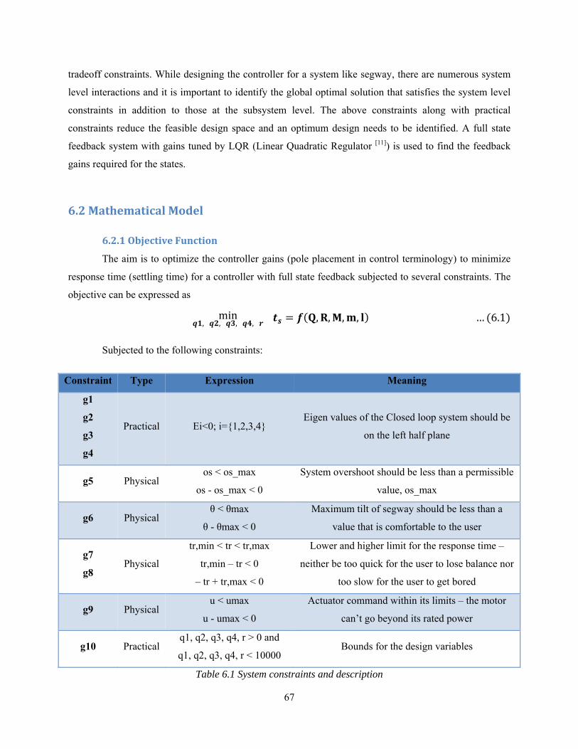
67

tradeoff constraints. While designing the controller for a system like segway, there are numerous system

level interactions and it is important to identify the global optimal solution that satisfies the system level

constraints in addition to those at the subsystem level. The above constraints along with practical

constraints reduce the feasible design space and an optimum design needs to be identified. A full state

feedback system with gains tuned by LQR (Linear Quadratic Regulator [11]) is used to find the feedback

gains required for the states.



The aim is to optimize the controller gains (pole placement in control terminology) to minimize

response time (settling time) for a controller with full state feedback subjected to several constraints. The

objective can be expressed as

min, , , ,

, , , , … 6.1

Subjected to the following constraints:

Constraint Type Expression Meaning

g1

g2

g3

g4

Practical Ei<0; i=1,2,3,4 Eigen values of the Closed loop system should be

on the left half plane

g5 Physical os < os_max

os - os_max < 0

System overshoot should be less than a permissible

value, os_max

g6 Physical θ < θmax

θ - θmax < 0

Maximum tilt of segway should be less than a

value that is comfortable to the user

g7

g8 Physical

tr,min < tr < tr,max

tr,min – tr < 0

– tr + tr,max < 0

Lower and higher limit for the response time –

neither be too quick for the user to lose balance nor

too slow for the user to get bored

g9 Physical u < umax

u - umax < 0

Actuator command within its limits – the motor

can’t go beyond its rated power

g10 Practical q1, q2, q3, q4, r > 0 and

q1, q2, q3, q4, r < 10000 Bounds for the design variables

Table 6.1 System constraints and description

68

The matrices

1 0 0 00 2 0 00 0 3 00 0 0 4

and are the weight matrices corresponding to the

four states and the control input. The qi corresponds to the importance of the ith state and r corresponds to

the importance given to the controller effort. When qi is large compared to the other gains, the LQR

algorithm calculates a gain matrix K such that the first state settles quickly while other states and input are

relaxed.

The LQR algorithm guarantees the stability of the system and hence robustness to stability is not

considered as an additional constraint to the problem. Practical bounds for the design variables are

selected after running trial optimization to avoid a null design space.

6.2.2 Plant Model

The dynamic model of the Segway for longitudinal motion [2, 3, 4] can be described with the help

of a simple schematic and equations of motion.

Figure 6.1 A schematic of Segway System [15]

Equations of motion

The equations of motion are based on the ‘inverted pendulum on a cart’ problem and formulated

using Lagrangian dynamics. The non-linear equations are

… 6.2

0 … 6.3

69

On linearization, the following equations can be obtained

1 … 6.4

1 … 6.5

In state space form, the model can be represented by

… 6.6

The above equation is of the form X AX Bu Fd where

0 1 0 0 0 0 0

0 0 0 1

0 0 0

01

01

… 6.7

The above linear system can be used to represent the Segway and Ei form the eigenvalues of the

matrix A. The control input is a force as shown in the diagram but the force is delivered as a torque by the

driving motor which can be calculated as follows

… 6.8

The controller is a simple full state feedback controller [16].

6.2.3 Design Variables and Parameters

The design variables are the variables that appear in the objective function. They are

(1) The state weight matrix variables , 4 variables 4

(2) The controller effort weight matrix 1 variable co the only input

The upper and lower bounds for the design variables are mentioned in the constraints table (Table 6.1).

The parameters in the model are

(1) Segway system mass M (depends on dimensions, material, size of motors, battery etc).

(2) Passenger mass m

70

(3) Height of center of mass l (depends on the passenger height and the segway frame height)

The system is modeled in MATLAB/SIMULINK where the optimization routine could be easily

called. The system is modeled in SIMULINK and called from MATLAB. Every time the model was

called for optimization, the solver crashed because the variables did not get updated for every run as the

model was called from within a function. However, using global variables and ‘set_param’ function to set

the parameters for the SIMULINK model solved the issue. A snapshot of the model in SIMULINK is

shown below.

Figure 6.2 SIMULINK model of the feedback system

6.3 Model Analysis

The objective function as well as the constraints is all nonlinear functions of the design variables.

The objective and constraints are determined from the SIMULINK model directly without using

analytical expressions. Hence a monotonicity analysis can’t be conducted in a direct manner and it is

important to make this analysis indirectly using engineering knowledge.

6.3.1 Behavior of the objective function and constraints

To analyze the dependency of the objective and constraints on each design variable (Xi), the

following plots have been shown. The design variables are the weights given to the states and control

effort. In the below analysis, it can be seen that the Eigen values constraint doesn’t make a big impact

because they were calculated using the LQR code in MATLAB which gives the best eigen values for a

stable system and hence they are met for any value of design variables. They can be considered

dominated by other active constraints.

71

Dependency on X1

Figure 6.3 shows how the settling time and the other constraints vary with increase in X1. As f

increases, g5, g6 and g9 decreases and the monotonicity relations are indicated in Table 6.2. The

maximum pendulum deflection angle (g6) and motor power required (g9) are a direct consequence of

overshoot (g5). If we need the system to be quick, we need to give a short power burst for the actuator

and hence overshoot increase which also means that the deflection is more. Hence the overshoot or motor

power could be an active constraint for the variable X1 bounding it from below. There is no upper bound

for this variable except for the practical constraint but that is of no significance since the objective

function increases as X1 increase.

Design Variable Expression Increase or Decrease?

X1 = q1

f ts

g1

g2

g3

g4

Ei<0; i=1,2,3,4

g5 os < os_max

os - os_max < 0

g6 θ < θmax

θ - θmax < 0

g7

g8


tr,min – tr < 0

– tr + tr,max < 0

g9 u < umax

u - umax < 0

g10 q1, q2, q3, q4, r > 0 and

q1, q2, q3, q4, r < 10000 Variable Bounds


*In the following Figures (Figure 6.3 – Figure 6.7), the top left subplot is the objective function and the

other subplots are the constraints

72


Dependency on X2

Figure 6.4 shows the effect of variable X2 on the settling time and the other constraints. With

increase in X2, f increases, g6 and g9 decreases and the monotonicity relations are indicated in Table 6.3.

The increase in X2 will be bounded by overshoot constraint (g5) which can’t go beyond a maximum

value. The decrease in X2 will be bounded by one of constraints g6 or g9 which has a maximum

permissible limit. Hence the variable X2 is well constrained by constraints g5, g6 or g9 which looks active

for the variable X2. The Eigen value constraints are well below the limited value and could be dominated

by the active constraints.

0 2000 4000 6000 8000 1000075.64

75.66

75.68

75.7

75.72

75.74

x1

sett

ling

time

in s

0 2000 4000 6000 8000 100004.2756

4.2756

4.2756

4.2757

4.2758

4.2758

x1

over

shoo

t in

%0 2000 4000 6000 8000 10000

1.1665

1.167

1.1675

1.168

1.1685

1.169

x1max

imum

pen

dulu

m a

ngle

in d

egre

es

0 2000 4000 6000 8000 1000013

13.5

14

14.5

15

15.5

x1re

spon

se t

ime

of p

endu

lum

in s

0 2000 4000 6000 8000 100000.1775

0.1776

0.1777

0.1778

0.1779

x1

mot

or p

ower

0 2000 4000 6000 8000 10000-8

-6

-4

-2

0

x1

Eig

en V

alue

s

73



X2 = q2

f ts

g1

g2

g3

g4

Ei<0; i=1,2,3,4

g5 os < os_max

os - os_max < 0

g6 θ < θmax

θ - θmax < 0

g7

g8


tr,min – tr < 0

– tr + tr,max < 0

g9 u < umax

u - umax < 0

0 2000 4000 6000 8000 1000075.645

75.65

75.655

75.66

x2

sett

ling

time

in s

0 2000 4000 6000 8000 100004.2757

4.2758

4.2758

4.2758

4.2758

4.2758

x2

over

shoo

t in

%

0 2000 4000 6000 8000 100001.1681

1.1681

1.1681

1.1681

x2max

imum

pen

dulu

m a

ngle

in d

egre

es

0 2000 4000 6000 8000 1000013

13.5

14

14.5

15

15.5

x2

resp

onse

tim

e of

pen

dulu

m in

s

0 2000 4000 6000 8000 100000.1778

0.1778

0.1778

0.1778

x2

mot

or p

ower

0 2000 4000 6000 8000 10000-10

-8

-6

-4

-2

0

x2

Eig

en V

alue

s

74

g10 q1, q2, q3, q4, r > 0 and



Dependency on X3

Figure 6.5 shows how the settling time and the other constraints vary with increase in X3. With

increase in X3, f decreases, g6, g8 and g9 increase and the monotonicity relations are indicated in Table

6.4. The increase in X3 will be bounded by one of response time (g7), motor power (g9) or maximum

pendulum angle (g6) which can’t go beyond their maximum values. The decrease in X3 will be bounded

by one of constraints g5 (overshoot) or g7 which has a maximum permissible limit. Hence the variable X2

is well constrained.


X3 = q3

f ts

g1

g2

g3

g4

Ei<0; i=1,2,3,4

g5 os < os_max

os - os_max < 0

g6 θ < θmax

θ - θmax < 0

g7

g8


tr,min – tr < 0

– tr + tr,max < 0

g9 u < umax

u - umax < 0

g10 q1, q2, q3, q4, r > 0 and



75


Dependency on X4


0 2000 4000 6000 8000 100000

20

40

60

80

x3

sett

ling

time

in s

0 2000 4000 6000 8000 100003.9

4

4.1

4.2

4.3

4.4

x3

over

shoo

t in

%

0 2000 4000 6000 8000 100000

5

10

15

x3max

imum

pen

dulu

m a

ngle

in d

egre

es

0 2000 4000 6000 8000 100000

5

10

15

x3

resp

onse

tim

e of

pen

dulu

m in

s

0 2000 4000 6000 8000 100000

0.5

1

1.5

2

x3

mot

or p

ower

0 2000 4000 6000 8000 10000-8

-6

-4

-2

0

x3

Eig

en V

alue

s

0 2000 4000 6000 8000 100000

100

200

300

400

x4

sett

ling

time

in s

0 2000 4000 6000 8000 100000

1

2

3

4

5

x4

over

shoo

t in

%

0 2000 4000 6000 8000 100000.2

0.4

0.6

0.8

1

1.2

x4max

imum

pen

dulu

m a

ngle

in d

egre

es

0 2000 4000 6000 8000 100006

8

10

12

14

16

x4

resp

onse

tim

e of

pen

dulu

m in

s

0 2000 4000 6000 8000 100000

0.05

0.1

0.15

0.2

x4

mot

or p

ower

0 2000 4000 6000 8000 10000-10

-8

-6

-4

-2

0

x4

Eig

en V

alue

s

76


X4 = q4

f ts

g1

g2

g3

g4

Ei<0; i=1,2,3,4

g5 os < os_max

os - os_max < 0

g6 θ < θmax

θ - θmax < 0

g7

g8


tr,min – tr < 0

– tr + tr,max < 0

g9 u < umax

u - umax < 0

g10 q1, q2, q3, q4, r > 0 and



Figure 6.6 shows how the settling time and the other constraints vary with increase in X4. With

increase in X4, f increases, g5, g6, g7 and g9 increase and the g8 increase. The monotonicity relations are

indicated in Table 6.5. The increase in X4 will be bounded by g8 (response time) which can’t go below a

minimum limit. The decrease in X4 will be bounded by one of constraints g5, g6, g7 or g9 which can’t go

beyond their maximum limits. Hence the variable X4 is well constrained.

Dependency on X5

The design variable r (X5) corresponds to the importance given to the control effort to keep it as

minimum as possible. As r increase, f increases because control effort will be lowered (g9 decreases) and

hence system takes a long time to settle. The constraint g6 also decreases because the system is not slowly

taken to steady state without much peaks and hence maximum deflection of pendulum decreases. The

overshoot increases but not very rapidly and the values are nearly constant around 4.31%. The decrease in

77

motor power g9 is very obvious. The response time (g7) increases as the system gets slower but we have

2 constraints for this quantity – the response time cannot be more than 8 and cannot be less than 2. Hence

g8 is an active constraint for X5 bounding it from above and one of g6 or g9 could be an active constraint

bounding X5 from below.


0 20 40 60 80 10050

100

150

200

250

x5

sett

ling

time

in s

0 20 40 60 80 100

4.28

4.29

4.3

4.31

4.32

x5

over

shoo

t in

%

0 20 40 60 80 1000.2

0.4

0.6

0.8

1

1.2

x5max

imum

pen

dulu

m a

ngle

in d

egre

es

0 20 40 60 80 10010

20

30

40

50

x5

resp

onse

tim

e of

pen

dulu

m in

s

0 20 40 60 80 1000.05

0.1

0.15

0.2

0.25

x5

mot

or p

ower

0 20 40 60 80 100-8

-6

-4

-2

0

x5

Eig

en V

alue

s

78


X5 = r

f ts

g1

g2

g3

g4

Ei<0; i=1,2,3,4

g5 os < os_max

os - os_max < 0

g6 θ < θmax

θ - θmax < 0

g7

g8


tr,min – tr < 0

– tr + tr,max < 0

g9 u < umax

u - umax < 0

g10 q1, q2, q3, q4, r > 0 and

q1, q2, q3, q4, r < 10000


6.3.2 Monotonicity Table

In order to summarize the monotonicity analysis for the system, a monotonicity table can be

constructed where the impact of each variable on the objective and constraint can be quickly observed and

analyzed. Table 6.7 shows the monotonicity relations for the subsystem concerned. The objective function

and the important constraints (possible active constraints) are considered. A + indicates monotonically

increasing relation and – indicates a monotonically decreasing relation. N indicates neutral (no change)

and NA indicates that monotonicity can’t be determined.

79

X1 X2 X3 X4 X5

f + + - + +

g5 - + NA - NA

g6 - - + - -

g7 N N - - +

g8 N N + + -

g9 - - + - -

Table 6.7 Monotonicity Table

The analysis performed above is not guaranteed to be accurate. The problem is a highly nonlinear

one and the absence of analytical relations for the objective and constraints makes it very hard to identify

the active constraints for each variable correctly. However, the monotonicity analysis for this subsystem

was based on physical intuition and can be considered a first insight into the problem even though it

doesn’t correctly reflect the shape of the feasible space.


Since the problem is not extremely non-monotonic, a first run of optimization was performed

using a gradient based method – fmincon routine in MATLAB. We are well aware that gradient based

methods converge to local minima and a good set of starting points are required. Hence 3 simulations are

performed with different starting points that reasonably covered the entire space. In order to compare the

gradient based and gradient free algorithms and to identify the appropriate optimization routine for the

given subsystem, a gradient free algorithm – Direct method was used in MATLAB. For all optimizations,

the following set of parameters and constants were used.

80

Quantity Value Units Description

Parameters

M 40 Kg Mass of the Segway System

m 120 Kg Mass of Payload

(Passenger and other load)

Rw 0.2 m Radius of wheel

Constants g 9.81 m/s2 Acceleration due to gravity

Table 6.8 System Parameters and Constants

6.4.1 Optimization using FMINCON

With any initial condition, the objective function was converged to a local minimum in less

number of iterations. The results for different initial conditions when optimized using fmincon are shown

below.

CASE 1:

Initial condition: X0 = [1, 1, 1, 1, 0.01]


0 5 10 15 20 254

6

8

10

12

14

16

18

20

22

24

Iteration

Fun

ctio

n va

lue


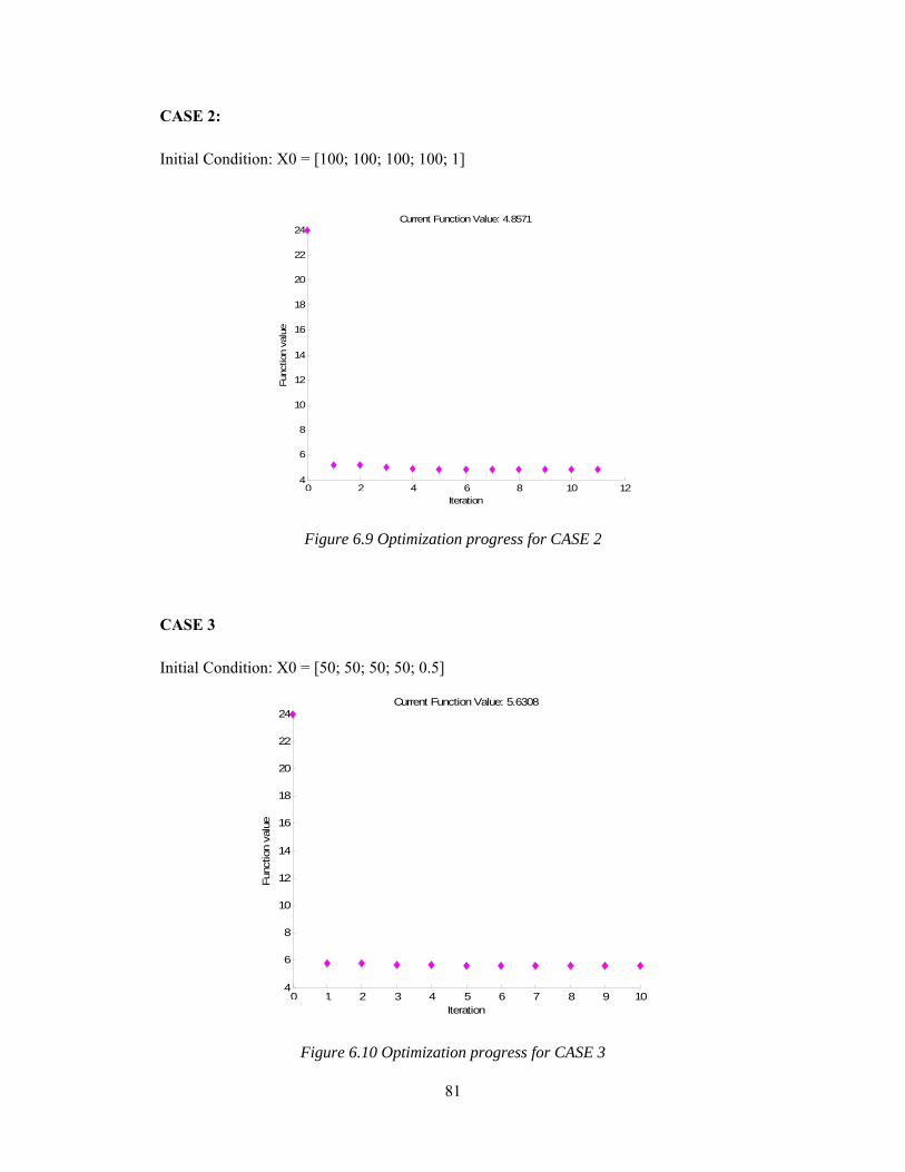
81

CASE 2:

Initial Condition: X0 = [100; 100; 100; 100; 1]


CASE 3

Initial Condition: X0 = [50; 50; 50; 50; 0.5]


0 2 4 6 8 10 124

6

8

10

12

14

16

18

20

22

24

Iteration

Fun

ctio

n va

lue


0 1 2 3 4 5 6 7 8 9 104

6

8

10

12

14

16

18

20

22

24

Iteration

Fun

ctio

n va

lue


82

Constraints Satisfied?

S – satisfied N – not satisfied

CASE 1

X0 = [1, 1, 1, 1, 0.01]

CASE 2

X0 = [100; 100; 100; 100; 1]

CASE 3

X0 = [50; 50; 50; 50; 0.5]

f* 4.8454 4.8571 5.6308

X*

X1 12.6780

X2 1.3690

X3 100.0000

X4 59.9586

X5 0.0100

X1 99.9016

X2 99.8811

X3 100.0000

X4 60.3112

X5 0.0100

X1 49.9902

X2 49.9887

X3 52.9391

X4 45.8658

X5 0.0100

g1

g2

g3

g4

-8.3151

-6.8283

-0.6130 + 0.4912i

-0.6130 - 0.4912i

S

-9.6929

-5.8654

-0.6125 + 0.4910i

-0.6125 - 0.4910i

S

-9.0589

-6.2527

-0.5236 + 0.4193i

-0.5236 - 0.4193i

S

g5 2.0000 S 2.0000 S 2.0000 S

g6 10.8214 S 10.8034 S

9.2109

S

g7

g8

1.7269

(upper active)

S

1.7269

(upper active)

S 1.7269 S

g9

1.6640

(lower active) S

1.6613

(lower active) S

1.4155

(lower active) S

Table 6.9 Comparison of fmincon optimization routine for different initial conditions

Table 6.9 compares the results of fmincon for different initial conditions. The solver also

mentioned about the upper and lower active constraints for the objective function. In all cases, the system

response time (constraints g7, g8) form the upper active bound while the motor power (constraint g9)

83

forms the lower active bound. This means that the bounds were active which dominates the constraints.

Future study can be conducted by extending the bounds until the constraints become active. However, if

the bounds are not considered, these constraints could be active which was identified by the monotonicity

analysis earlier.

6.4.2 Optimization using DIRECT METHOD and Combined Optimization

Given the same parameters and constants, the optimization problem is solved by a gradient free

method – Direct method and it was observed that the direct method can be time consuming. It takes about

10 times the time taken by fmincon routine. Also, the direct method converged to a global optimum but

that was less than what fmincon could converge.

We are aware that the direct method is a globally convergent algorithm and fmincon is a locally

convergent algorithm. It means that even if direct method fails to find a solution that is better than that of

fmincon, it gives a sense of global optimum. Without an initial condition, it converges to a global

optimum region whereas fmincon converges to a local optimum given a starting condition. On trying with

several starting conditions, only if we are fortunate that fmincon will find a global optimum. This

behavior can be explained with the help of the figure below.

Figure 6.11 Working principle behind global optimization (Direct) and local optimization (fmincon)

If we consider the scenario in the figure above, the direct method can be used to converge to a

global optimal space (dark black circle). If this region is used as an initial condition for fmincon, we can

84

converge to a local optimum in the global optimum space (yellow point). This solution can be considered

as a global minimum. An alternate approach could be to start with several initial conditions for fmincon

and end at the best solution. However such a solution cannot be guaranteed to be a global optimum. For

the controls subsystem, the solution obtained using combined optimization is better than the optimum

values of both methods used separately. The results of the direct method and the improved solution using

fmincon can be shown in the table below.

Constraints Satisfied?

S – satisfied N – not satisfied

Direct method Fmincon with initial condition from direct method

f* 5.1748 4.8423

X*

X1 34.4602

X2 1.3244

X3 99.9925

X4 96.3409

X5 0.0101

X1 34.4494

X2 2.1005

X3 100.0000

X4 59.9711

X5 0.0100

g1

g2

g3

g4

-8.5459

-6.6943

-0.6356 + 0.4531i

-0.6356 - 0.4531i

S

-8.3250

-6.8232

-0.6129 + 0.4911i

-0.6129 - 0.4911i

S

g5 1.2387 S 1.2387 S

g6 10.4783 S 10.8194 S

g7

g8

1.7269

(upper active) S

1.7269

(upper active) S

g9 1.6108 S 1.6636 S

Table 6.10 Comparison of fmincon and direct method optimization routines

85


The global optimum of an optimization problem is valid only for the given set of variables and

parameters. It is highly likely that the parameters vary a lot due to changes in the requirements as well as

uncertainty in measurements. Hence it is important to understand how the global optimum varies with

variations in the system parameters. For instance, a Segway system can’t be designed only for a person

with a particular weight and height. It has to be robust and satisfactorily function to a wide range of users.

Hence the variation of passenger mass (m in the model) and passenger height (which affects center of

mass height l in the model) on the global optimum are studied. For the following parametric studies, it has

been observed that the solver gave optimum results with all constraints well within its limits and the plots

have been generated only after the optimum was found.

6.5.1 Passenger Mass

The passenger mass is varied between 80 and 140 Kg in steps of 10 and the variation in the

objective and constraints are analyzed as shown below. It can be observed that if the passenger weight is

increased, the settling time increases. Also the motor power required increases along with overshoot. But

the max pendulum angle is decreased. This can be realized physically where the motor need more power

to move greater load and the system takes more time to settle because of overshoot. This behavior can be

expected for increase in passenger mass in any range.

Figure 6.12 Variation of settling time with Passenger Mass

80 90 100 110 120 130 140

4.85

4.9

4.95

5

5.05

5.1

5.15

5.2

5.25

5.3

5.35

Passenger Mass in kg

Set

tling

Tim

e in

s

86

Figure 6.13 Variation of system constraints with Passenger Mass

6.5.2 Passenger Height

The passenger height affects the height of center of mass of the system directly. By varying the

value of l between 0.4 m to 1.1 m in steps of 0.1 m (which corresponds to about 80 cms to 220 cms in

steps of 20 cms in terms of passenger height), the variation of objective and constraitns are analyzed as

shown below.

Figure 6.14 Variation of Settling time with Passenger center of mass height

80 90 100 110 120 130 1400.8

0.9

1

1.1

1.2

1.3

1.4

1.5


Ove

rsho

ot in

%

80 90 100 110 120 130 14010

10.2

10.4

10.6

10.8

11

11.2

11.4

11.6


Max

Pen

dulu

m A

ngle

80 90 100 110 120 130 1400.5

1

1.5

2

2.5

3


Res

pons

e Tim

e

80 90 100 110 120 130 1401.3

1.4

1.5

1.6

1.7

1.8


Mot

or P

ower

Req

uire

d in

KW

0.4 0.5 0.6 0.7 0.8 0.9 1 1.1

5.1

5.15

5.2

5.25

5.3

5.35

5.4

5.45

5.5

Passenger CG Height in m

Set

tling

Tim

e in

s

87

Figure 6.15 Variation of constraints with Passenger center of mass height

From the above Figures, we can observe that if the passenger is tall, the settling time increases

while overshoot, pendulum max angle and the motor power reduces. This might be because the center of

mass plays an important role in balancing the pendulum torque and the motor torque. For the same mass

and greater ‘perpendicular radius’, we get a greater driving torque and the motor only needs to give

sufficient torque to balance the system and hence a lower value. This behavior can be expected for

increase in passenger CG height in any range.


The optimization study using fmincon and direct method resulted in a global optimum solution.

The complete optimization study can be summarized in the following figure.

0.4 0.5 0.6 0.7 0.8 0.9 1 1.11.1

1.15

1.2

1.25

1.3

1.35


Ove

rsho

ot in

%

0.4 0.5 0.6 0.7 0.8 0.9 1 1.1

10.2

10.3

10.4

10.5

10.6


Max

Pen

dulu

m A

ngle

0.4 0.5 0.6 0.7 0.8 0.9 1 1.10.5

1

1.5

2

2.5

3


Res

pons

e Tim

e

0.4 0.5 0.6 0.7 0.8 0.9 1 1.11.56

1.57

1.58

1.59

1.6

1.61

1.62

1.63


Mot

or P

ower

Req

uire

d in

KW

88

Figure 6.16 Summary of optimization study

From the above figure, it can be observed that the design variable X3 that corresponds to the

weight given to the angular velocity of the pendulum state has reached its upper bound. If the value of

weight for any state is high, it means that that state will settle down soon. Hence when X3 reaches its

upper bound, it means that the response time (constraints g7 and g8) is quick and hence the low settling

time. This also implies that the variable bound on X3 itself is an active constraint limiting the objective

function. However, the settling time also depends on the other states which affect overshoot, controller

effort etc. and it can be said that the optimum is reached only if the value of X3 hits its upper bound.

Also, the value of X5 reaches its lower bound. This means that the system is trying to settle down

quickly and doesn’t give any importance to the controller effort which increases the motor power required

to control the system. The value of X5 hitting its lower bound also means that the constraint on motor

power required (2 KW) is higher than that corresponding to the lowest value of X5. If the lower bound is

reduced, then there might be a case where the constraint would be active and limit the value of X5.The

values of the other variables at the optimum are interior to the bounds and hence the optimum obtained is

an interior solution. The active bounds were identified by fmincon and have been shown in Table 6.9.

The control system performance is compared to the uncontrolled system and is shown in the

figure below

89

Figure 6.17 Comparison of optimal controller to that of the base controller

Figure 6.17 shows the response of the system velocity when given a step change in the platform

tilt. It can be observed from the figure above that the optimal controller has a quicker response and less

overshoot.

Future work can focus on varying the active bounds and shrinking the inactive bounds to see the

solution limits. Also, the present model captures only longitudinal dynamics and it would be interesting to

add a more complete steering model to find if any active bounds on the other variables arise.

6.7 SystemLevel Tradeoffs

All the above tasks of finding the optimum objective function value are with respect to the given

set of parameters and constraints. However when the above subsystem is integrated to the other

subsystems to complete the Segway system, system level interactions are expected that could vary the

parameters, constants as well as the constraint limits.

Time (sec)

Am

plitu

de

0 5 10 15 20 25 30 35 400

5

10

15

20

25

optimal design

base design

90

For instance, the objective of this subsystem is to minimize the settling time. One of the active

constraints is the motor max power which has an upper limit of 2 KW. At a system level, this value could

increase or drop depending on the optimum motor scaling factor that is determined by the electrical

subsystem. Hence the global minimum from this subsystem may not remain the same at a system level

and hence a slower or faster system could result depending on the subsystem’s optimal design. Also, the

parameters used in the model come from other subsystems during system study and hence the solution is

expected to change on integration with other subsystems. For example, the system mass is a parameter

used in this model which is a sum of the structure mass (from structure subsystem) and electrical system

mass (from electrical subsystem) and as the subsystems are optimized, these parameters vary and will

have an effect on the optimal design of the control system.

Another instance could be a conflict with the electrical subsystem for the motor and battery

rating. An active constraint, the small response time requirement of the system can demand for a large

electric motor which might not be possible because it increases the weight and cost of the overall system.

Hence the constraint may not be satisfied at a system level. It may also result in a situation where the

structure can be relaxed by a little reducing weight and cost thereby giving resources to buy a larger

motor that can satisfy the constraints. These issues need to be examined during system integration and

constraint relaxation or elimination might have to be done to accommodate the most important needs.

91

7. System Integration Study

The optimization study at a subsystem level has been done and valuable insights have been

gained. The objective of this project is to optimize the Segway as a system and not just the subsystems.

Hence it is important to understand the behavior of every subsystem as well as the interactions between

them, the causality and the tradeoffs. When the four concerned subsystems are combined, the system

model has 20 design variables, 34 parameters and 4 constants. A monotonicity analysis for the system

may not be done because enough insights on the subsystems have been gained and it would be redundant

if a system level monotonicity analysis is performed. The major tasks in a system integration study are

(1) Identifying the system level interactions

(2) Linking the subsystem models to create the complete system model.

(3) Formulating and solving the optimization problem

Each of these will be discussed in the following sections.

7.1 System Interactions

There are four subsystems for the Segway – Structure, Electrical, Vibrations and Controls and all

of these interact with each other. The system level interactions is pictured as shown below

Figure 7.1 System interactions

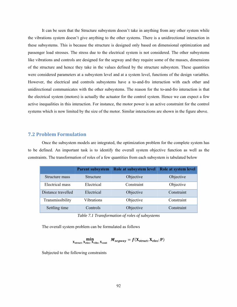
92

It can be seen that the Structure subsystem doesn’t take in anything from any other system while

the vibrations system doesn’t give anything to the other systems. There is a unidirectional interaction in

these subsystems. This is because the structure is designed only based on dimensional optimization and

passenger load stresses. The stress due to the electrical system is not considered. The other subsystems

like vibrations and controls are designed for the segway and they require some of the masses, dimensions

of the structure and hence they take in the values defined by the structure subsystem. These quantities

were considered parameters at a subsystem level and at a system level, functions of the design variables.

However, the electrical and controls subsystems have a to-and-fro interaction with each other and

unidirectional communicates with the other subsystems. The reason for the to-and-fro interaction is that

the electrical system (motors) is actually the actuator for the control system. Hence we can expect a few

active inequalities in this interaction. For instance, the motor power is an active constraint for the control

systems which is now limited by the size of the motor. Similar interactions are shown in the figure above.

7.2 Problem Formulation

Once the subsystem models are integrated, the optimization problem for the complete system has

to be defined. An important task is to identify the overall system objective function as well as the

constraints. The transformation of roles of a few quantities from each subsystem is tabulated below

Parent subsystem Role at subsystem level Role at system level

Structure mass Structure Objective Objective

Electrical mass Electrical Constraint Objective

Distance travelled Electrical Objective Constraint

Transmissibility Vibrations Objective Constraint

Settling time Controls Objective Constraint

Table 7.1 Transformation of roles of subsystems

The overall system problem can be formulated as follows

, , ,

, ;

Subjected to the following constraints

93

Constraint Type Expression Meaning

Structure Subsystem

g1 Practical Cost < cost_max Low cost

g2 Physical Frame stress < yield stress Avoid device material failure

g3 Physical Wheel stress < yield stress Avoid device material failure

g4 Physical Platform stress < yield stress Avoid device material failure

g5 Practical Platform height < wheel height

– safety distance Keep user’s safe and better contained

g6 Physical Ground clearance < lowest non-

wheel part Ground clearance

g7 Practical width < width_max Practical width

g8 Practical width > width_min Humans must be able to use it comfortably

g9 Practical length < length_max Practical length

g10 Practical length_min < length Humans must be able to use it comfortably

g11 Practical Platform height < platform

height_max A human must be able to step up to it

g12 Physical inner frame diameter < outer

frame diameter The pipe cannot be physical otherwise

g13 Practical outer frame diameter < outer

frame diameter_max

A human must be able to position one foot on

either side

g14 Practical Wheel radius < wheel

radius_max

The wheel radius cannot pose a danger to the

user

g15 Practical frame deflection < frame

deflection_max Practical usability

g16 Practical wheel contact min < wheel

contact Minimum contact area with the ground


94

g26 Practical Distance min < Distance

Minimum range of segway required from a

fully charged battery (Scaled down for 10 sec

run)

g27 Practical Efficiency min < Efficiency Motor operating efficiency should be above

the minimum

g28 Practical Imax < max Imax Current in the circuit should be within limits

g29 Practical Motor Cost < max Motor cost Low cost

g30 Practical Velocity > min Velocity Speed to be greater than minimum required

value


g17 Practical transmissibility < 0.4 max allowable transmissibility

g18 Practical transmissibility > 0 non-negative transmissibility

Controls Subsystem

g19 Physical System overshoot < max

permissible limit System should not oscillate

g20 Physical Max tilt of platform < max

permissible value

Segway should not tilt too much for user to

lose balance

g21 Physical Response time < max value Response of Segway should not be too slow

g22 Physical Response time > min value Response of Segway should not be too quick

g23 Physical Actuator power limit < max

value

Controller effort should be less than electrical

system’s maximum ability

g24 Practical Eigen values should be negative Eigen values should be on the left half plane

for stability

g25 Physical Settling time < max permissible

value Control response should settle quickly

This problem has some design variables that do not appear in the objective function such as the

spring and damper constants, controller gains etc (they appear only for the constraints and is interesting

95

when the constraints are active). For instance, the settling time is an active constraint for the system

problem and depends on the controller gains which do not appear in the objective function. This

constraint however does affect the optimum design variable values and hence cannot be eliminated from

the analysis according to monotonicity principle 2.

7.3 Optimization Approaches

The optimization problem for the system was not straight forward and a simple application of any

single available algorithm did not result in a feasible solution. Hence the following methods were

attempted.

7.3.1 First Attempt with Fmincon

Several attempts using fmincon failed to converge to a feasible region. On observing the function

progress, it was seen that the objective function did not converge at all. Instead of decreasing, the function

values increased at certain iterations. The following plot shows the function history plot from fmincon.

Figure 7.2 fmincon: objective function vs iteration

The behavior was the same even after about 200 function evaluations and it was concluded that

fmincon wouldn’t return to feasible space and hence we did not proceed with further iterations. One

reason for this behavior could be that fmincon is based on sequential quadratic programming (SQP) with

active set strategy which does a quadratic approximation of the objective function and linear

approximation of the constraints. Hence it might be possible that the highly nonlinear constraints were

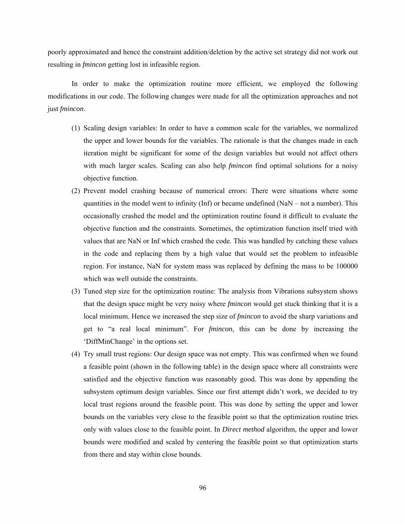
96

poorly approximated and hence the constraint addition/deletion by the active set strategy did not work out

resulting in fmincon getting lost in infeasible region.

In order to make the optimization routine more efficient, we employed the following

modifications in our code. The following changes were made for all the optimization approaches and not

just fmincon.

(1) Scaling design variables: In order to have a common scale for the variables, we normalized

the upper and lower bounds for the variables. The rationale is that the changes made in each

iteration might be significant for some of the design variables but would not affect others

with much larger scales. Scaling can also help fmincon find optimal solutions for a noisy

objective function.

(2) Prevent model crashing because of numerical errors: There were situations where some

quantities in the model went to infinity (Inf) or became undefined (NaN – not a number). This

occasionally crashed the model and the optimization routine found it difficult to evaluate the

objective function and the constraints. Sometimes, the optimization function itself tried with

values that are NaN or Inf which crashed the code. This was handled by catching these values

in the code and replacing them by a high value that would set the problem to infeasible

region. For instance, NaN for system mass was replaced by defining the mass to be 100000

which was well outside the constraints.

(3) Tuned step size for the optimization routine: The analysis from Vibrations subsystem shows

that the design space might be very noisy where fmincon would get stuck thinking that it is a

local minimum. Hence we increased the step size of fmincon to avoid the sharp variations and

get to “a real local minimum”. For fmincon, this can be done by increasing the

‘DiffMinChange’ in the options set.

(4) Try small trust regions: Our design space was not empty. This was confirmed when we found

a feasible point (shown in the following table) in the design space where all constraints were

satisfied and the objective function was reasonably good. This was done by appending the

subsystem optimum design variables. Since our first attempt didn’t work, we decided to try

local trust regions around the feasible point. This was done by setting the upper and lower

bounds on the variables very close to the feasible point so that the optimization routine tries

only with values close to the feasible point. In Direct method algorithm, the upper and lower

bounds were modified and scaled by centering the feasible point so that optimization starts

from there and stay within close bounds.

97

Feasible design variables objective function

X1=0.2 X2=0.035 X3=0.01 X4=0.45 X5=0.63

57.41 kg X6=0.084 X7=0.1 X8=0.951 X9=24001 X10=3000

X11=200024 X12=1500 X13=34.46 X14=1.32 X15=100

X16=96.34 X17=0.01 X18=1.04 X19=2.92 X20=0.73

Table 7.2 Showing feasible design and the objective corresponding to it

After making the above changes, we realized that fmincon worked in a much better way. The

figure below shows that the objective converged but still couldn’t find a feasible point.

Figure 7.3 fmincon: objective function vs iterations

Only a few constraints were violated and the model never crashed but the process was too slow to

be run for hundreds of iterations. If run for many hundreds of iterations, fmincon would have settled in a

feasible space but given the additional active constraint, the project deadline, we had to find a better

approach.

7.3.2 Direct Method Algorithm

Direct method worked really well for some of our subsystems (controls and vibrations) and so we

tried it for the system level optimization. The direct method is a derivative free globally convergent

algorithm works really well for problems with less number of design variables. As the number increases,

the number of iterations required to solve the problem increases exponentially. For the Segway system,

there were 20 design variables and even after running for 7500 function evaluations, a feasible solution

could not be found.

98

7.3.3 Nomad Algorithm

The nomad is a derivative free algorithm that worked well for the vibrations subsystem was used

to solve the system problem but with no use. Nomad too couldn’t find a feasible solution.

7.3.4 Simulated Annealing

Simulated Annealing is a quasi-global derivative free algorithm and is known to work well for

large dimension problems. Simulated Annealing gave a solution which violated the constraints. This

might be due to the fact that simulated annealing doesn’t have a good constraint handling technique. The

constraints are multiplied by a penalty factor and added to the objective function. Hence there is no

guarantee that the optimum would not violate all constraints. There are many parameters to be tuned for

good performance such as the penalty weights and temperature cooling schedule. The statement above

was based on the knowledge given in the lecture by John Whitefoot on derivative free algorithms.

7.3.5 Sequential Aptimization of Subsystems

As discussed in the system interaction section (Figure 7.1), the Segway system doesn’t have too

many 2-way type of iteration. Most of the interactions are 1-way and hence it is very easy to optimize the

subsystems separately and sequentially depending on the direction of interaction.

The structure subsystem was optimized first using fmincon and the optimum defined the

parameters for the remaining subsystems. Using the results from structure system, the electrical system

was optimized (If there were any constraints of system-1 that depend on the optimum design variables of

system-2, it is necessary to go back and check the validity of the constraints of system-1 using the output

from system-2). The output of the electrical system were fed to the control system and optimized

separately. However, an active constraint of the controls subsystem, the motor maximum power which

affects the response time of the segway, was defined by the electrical system. In the first loop, the

maximum power was very less that the controls subsystem could not find a feasible solution. This was

fixed by going back to the electrical system and adding another constraint so that the electrical system

produces at least the required power by the control system. The new optimum of electrical system is fed

again to the control system and an optimum design was found. Finally, the vibrations subsystem was

optimized taking the subsystem optimum of the others.

99

In this way, an iterative procedure was employed and the overall system optimum was found that

satisfied all the constraints and the objective function value being very low (this value was much lower

that the feasible solution). This is compared in the table shown below

Feasible design variables Initial Feasible

point

Sequential

optimum

X1=0.152 X2=0.035 X3=0.035 X4=0.45 X5=0.63

57.41 kg 34.4 kg X6=0.085 X7=0.1 X8=0.951 X9=30000 X10=3001.29

X11=200000 X12=1500 X13=34.45 X14=2.03 X15=100

X16=56.36 X17=0.01 X18=0.55 X19=0.71 X20=2.17

Table 7.3 Comparing the feasible design and the sequential optimum objective functions

The combined subsystem optima resulted in a feasible point and not the overall system optimum

and there were system conflicts which were resolved using the sequential optimization.

7.3.6 Second Attempt with Fmincon

The above optimum seemed like a really good solution. However, we wanted to observe the

behavior of fmincon with the above value as the starting point. To our surprise, fmincon worked well and

found a better point after 3 iterations. This solution cannot be termed as the global minimum since

fmincon only finds local minimum and it depends on the initial condition. Hence this is the best solution

that can be obtained for the segway system based on the above approaches and the given time frame. The

progress of fmincon can be shown in the figure below and this solution is compared with the previously

found solutions.

Figure 7.4 fmincon: objective function with iterations

100

Feasible design variables

Initial

Feasible

point

Sequential

optimum

Sequential

+

fmincon

X1=0.152 X2=0.035 X3=0.035 X4=0.45 X5=0.63

57.41 kg 34.4 kg 32.08 kg

X6=0.085 X7=0.1 X8=0.95 X9=30000 X10=3001.29

X11=200000 X12=1500 X13=34.45 X14=2.03 X15=100

X16=56.36 X17=0.01 X18=0.37 X19=0.69 X20=2.17

Table 7.4 Comparing the objective function values of the feasible design, the sequential optimum and the

fmincon solution from sequential optimum

7.4 Numerical Results

As discussed earlier, the optimum of all the subsystems is just a feasible solution and not an

optimal solution for the system problem. On examining the nature of the problem, a better feasible point

was found using the approaches discussed in the previous section. This solution was considered a local

optimum and the results are shown below.

Variable System Subsystem Variable System Subsystem

Wheel radius 0.152 m 0.152 m Scaling factor for

battery Ah 2.17 0.73

Wheel thickness 0.035 m 0.035 m Suspension spring

stiffness 30000 Nm 24001 Nm

Platform width 0.035 m 0.035 m Suspension damper

coefficient

3001.29

Ns/m 3000 Ns/m

Platform thickness 0.45 m 0.45 m Tire stiffness 200000 Nm 200024

Nm

Platform length 0.63 m 0.63 m Tire damping

coefficient 1500 Ns/m 1500 Ns/m

101

Inner frame diameter 0.085 m 0.084 m Controller gain q1 34.45 34.46

Outer frame diameter 0.1 m 0.1 m Controller gain q2 2.03 1.32

Handlebar height 0.951 m 0.951 m Controller gain q3 100 100

Scaling factor for

motor 0.37 1.04 Controller gain q4 56.36 96.34

Scaling factor for

battery voltage 0.69 2.92 Controller gain r 0.01 0.01

Table 7.5 Listing the optimal design at the system and the subsystem levels

Objective function System level Subsystem level

Structure Mass 22.06 kg 22.36 kg

Electrical System Mass 10.02 kg 19.02 kg

Vehicle Range 20.1 km

(constraint)

23.3 km

(maximize)

Transmissibility 0.26 0.38

Settling Time 7.0 sec 4.84 sec

Table 7.6 Listing the objective function values at the system and the subsystem levels

The optimal design for the system is compared with the optimal design of the subsystems as

shown in table 7.5 and the objective function values are compared in table 7.6. It can be observed that the

subsystem level optimal design is not the same as that of the system level optimal design and the

difference gives an idea about the system interactions that changed the feasible design space. From table

7.6, it can also be seen that the objective functions of all the subsystems improved when integrated with

the system except for the settling time which got a hit. The settling time is an active constraint for the

system which moved to its upper bound (7 seconds) at the optimum. While at the subsystem level, it was

an objective function and was minimized to 4.8 seconds. It is compromised by about 2 seconds in order to

improve the objectives of the other subsystems. Also, the mass of the electrical subsystem has reduced

since the range which was the objective function at the subsystem level has become a constraint while the

subsystem mass which was earlier a constraint has become the objective in the system level. Hence, the

102

optimizer has minimized the mass while meeting the set constraints. This is a good example of a system

level trade off caused due to system interaction. Below are a few important results for the whole system.

The system weight seems to be comparable to the ones available in the market [17]. The cost cannot be

compared because the below table represents the cost of the material and the motor. Costs owing to

development, manufacturing, marketing etc. are not included and doesn’t give a full picture about the cost

of the segway.

Final system mass is: 32.08 kg

Final material cost is: $ 97.06

Final motor cost is: $ 329.14

Table 7.7 Summary of final costs

7.5 Conclusion

The Segway system was an ideal case study to conduct design optimization. The nature of system

interaction and the complexities of each subsystem made it feasible for a 4-month course project. There

were a few system assumptions and approximations being made during the modeling phase that reduced

the complexity of the problem but at the same time had enough to capture the interesting behavior.

Every subsystem was modeled from scratch except for the electrical system (taken from an

existing model) which gave us a chance to understand the problem completely and model analysis helped

in gaining an insight into the optimization problem. Even though few of the subsystems had a highly non-

linear (black box type) model, critical examination of the objective function dependency on the variables

have been performed and an indirect monotonicity analysis have been performed.

During subsystem optimization, we learned how to use the optimization routine to solve the

problem, handle constraints, debug codes, use the theory learned in class to sensibly set bounds, select

initial conditions, time-steps etc. and understand the validity of the results. The difference between

gradient based and derivative free algorithms have been understood.

Understanding of the system level interactions and causality helped in selecting the appropriate

algorithm for the system level optimization and arrive at a feasible solution. The system integration was

not straight forward and hence valuable experience was gained while solving the system problem.

103

8. References [1] Picture source: http://co2calculator.wordpress.com/2008/10/

[2] Analysis of Stress and Strain in a Vehicle Wheel;

http://pep.metapress.com/content/y30x465434780n75/

[3] Specific Beam Loading;

http://www.efunda.com/formulae/solid_mechanics/beams/casestudy_display.cfm?case=cantilever_endloa

d#target

[4] Structural Beam Bending Equations;

http://www.engineersedge.com/beam_bending/beam_bending9.htm

[5] Ugural, A.C. Stresses in Beams, Plates and Shells 2009

[6] SIMULINK model and maps of Toyota Prius provided in ME 555-009 course

[7] Power-to-weight ratio data

http://en.wikipedia.org/wiki/Power-to-weight_ratio#Electric_Motors.2FElectromotive_Generators

[8] Cost of Battery Power

http://corrosion-doctors.org/Batteries/cost.htm

[9] Pareto optimization of a five-degree of freedom vehicle vibration model using a multi-objective

uniform-diversity genetic algorithm by N. Nariman-Zadeh et al.

[10] Bounds on Spring Constants and Damper Coefficients: Vehicle suspension optimization,

Mathematical and Computer Modelling, Volume 11, 1988, Pages 946-949, P. Pintado, F.G. Benitez

[11] Theory on LQG, http://en.wikipedia.org/wiki/Linear-quadratic_regulator

[12] Theory on inverted pendulum problem, http://en.wikipedia.org/wiki/Inverted_pendulum

[13] Lecture notes on Inverted pendulum problem, EECS 560, Prof. Grizzle

104

[14] Adam Cardi, “Design of RC Segway”

[15] Source of figure, http://en.wikipedia.org/wiki/Inverted_pendulum

[16] Inverted pendulum modeling, http://www.engin.umich.edu/group/ctm/examples/pend/invSS.html

[17] Typical weight of a segway can be found here: http://www.speed-sports.com/segway/index.html

105

9. Appendix

9.1 Structrural Subsystem

9.1.1 MATLAB Codes

Below are the codes used for the fmincon function.

% The following script is the file which sets up an optimization using % the fmincon function. Other subroutines are called and their % descriptions and comments may be found in those files % % Nomenclature % Note: All units are in kg, N, m, depending on the dimension in % question % % Objective % smax = maximum stress from analytical calculations % Variables (x) % x(1) = r = wheel radius % x(2) = t = wheel thickness % x(3) = hp = platform thickness % x(4) = lp = platform length % x(5) = wp = platform width % x(6) = dfi = inner frame diameter % x(7) = dfo = outer frame diameter % x(8) = hh = handlebar height % % Parameters % A = maximum cost in USD for the materials of the structure % B = minimum safety distance from top of platform to top of wheels % C = minimum ground clearance % D % E = maximum device footprint width % F = maximum device footprint length % G = comfortable low reach hand height % H = human foot width % I = distance between medial sides of feet % J = human foot length % K = comfortable human step height % L = comfortable high reach hand height % hm = motor height % rho = density of chosen material % nu = Poisson's ratio of chosen material % c = cost per volume of chosen material

106

% yield = yield strength of chosen material % V = total volume of structure clear all close all % Initialize parameters A = 450; B = .1; C = .1; E = .7; F = .5; G = .951; %Female low - This captures over 95% of the population H = .08; %This captures over 95% of the population I = .5; %This is the max distance a rider should have to spread his or her feet J = .3; %This captures over 95% of the population K = .4; %This makes for a manageable step height L = 1.1898; %Male high - This captures 95% of the population hm = .05; %rho goes here %nu %c %yield Ph = 300; %This is the load at the handlebars Pb = 180000; %This is the load at the platform %Elastic N = .0005; %Maximum handlebar deflection % In order to get information for a specific material, that must be % specified. The number chosen for the variable k will correspond to one % of six materials as follows: % k = 1, Stainless Steel 304 % k = 2, Cold Drawn Steel 1045 % k = 3, Steel 4130 annealed at 865C % k = 4, Aluminum 6061 T6 % k = 5, Aluminum 7075 T6 % k = 6, Hexcel Carbon Fiber. Many material properties associated with % this particular material are inexact and depend on dimensions and % application method. Any results should be considered VERY rough % estimates of how the carbon fiber would perform. % Set material %%%%%%%%%%%% %%%%%%%%%%%% k = 6; %%%%%%%%%%%%% %%%%%%%%%%%%% [c nu rho yield Elastic] = Findprops(k); global Params; Params = [A;B;C;E;F;G;H;I;J;K;L;hm;rho;nu;c;yield;Ph;Pb;Elastic;N]; % global sParams; % sParams = Params./Params;

107

Amatrix = []; bvec = []; Aeq = []; beq = []; lb = [0 0 0 0 0 0 0 G]; ub = [1e6 1e6 1e6 1e6 1e6 1e6 I L]; options = optimset('Display','iter',... % output 'TolX',0.001,... % convergence tolerance on design variables 'TolFun',0.0001,... % convergence tolerance on objective function 'TolCon',0.001,... % convergence tolerance on constraints 'MaxIter',1400,... % maximum number of iterations 'DiffMinChange',0.2,... % minimum finite difference (for calculating gradients) 'DiffMaxChange',0.2,... % maximum finite difference (for calculating gradients) 'LargeScale','off'); % large scale optimization (usually should be set to OFF) global x0; x0 = [.25,.1,.1,.75,.5,.05,.1,.5]; % initial starting point % xscaled0 = x0./x0; [xopt,fval,exitflag,ouput] = fmincon('FUNmass',x0,Amatrix,bvec,Aeq,beq,lb,ub,'NONLCON'); xopt function [g,h]=NONLCON(x) global Params % inequality constraints r = x(1); %= wheel radius t = x(2); %= wheel thickness hp = x(3); %= platform thickness lp = x(4); %= platform length wp = x(5); %= platform width dfi = x(6); %= inner frame diameter dfo = x(7); %= outer frame diameter hh = x(8); %= handlebar height A = Params(1); B = Params(2); C = Params(3); E = Params(4); F = Params(5); G = Params(6); H = Params(7); I = Params(8); J = Params(9); K = Params(10); L = Params(11); hm = Params(12);

108

rho = Params(13); nu = Params(14); c = Params(15); yield = Params(16); Ph = Params(17); Pb = Params(18); Elastic = Params(19); N = Params(20); V = 2*pi*r^2*t + lp*hp*wp + pi*hh*((dfo/2)^2 - (dfi/2)^2); pipestress = 32*Ph*hh*dfo/(pi*(dfo^4 - dfi^4)); wheelstressy = Pb/(pi*r*t); platfstress = FUN3(x); % flexrig = Elastic*t^3/(12*(1-nu^2)); % wheeldefl1 = Pt*r^2/(16*pi*flexrig)*(3+nu)/(1+nu); % wheelI = (pi/4)*(6*r*t^3); % wheeldefl2 = Pt*r^3/(3*Elastic*wheelI); % wheeldefl = max(wheeldefl1, wheeldefl2); % wheelstressx = 3*Pt/(2*pi*t^2)*(1-nu); PipeI = pi*(dfo^4 - dfi^4)/64; pipedefl = Ph*hh^3/(3*Elastic*PipeI); g=[(V*c - A)/A; (pipestress - .8*yield)/yield; (wheelstressy - .8*yield)/yield; (platfstress - .8*yield)/yield; -r + .5*hp + B; -r + .5*hp + hm + C; wp + 2*t - E; 4*H + dfo - wp/1.5; lp - F; 1.5*J - lp; r + .5*hp - K; dfi - dfo; dfo - I; r - .5*hp - G; % wheeldefl - M; % wheelstressx - .8*yield; pipedefl - N; .05 - t/(2*t + wp); ]; % equality constraints h=[ ];

function [g,h]=NONLCON(x) global Params % inequality constraints r = x(1); %= wheel radius t = x(2); %= wheel thickness

109

hp = x(3); %= platform thickness lp = x(4); %= platform length wp = x(5); %= platform width dfi = x(6); %= inner frame diameter dfo = x(7); %= outer frame diameter hh = x(8); %= handlebar height str_A = Params(1); str_B = Params(2); str_C = Params(3); str_E = Params(4); str_F = Params(5); str_G = Params(6); str_H = Params(7); str_I = Params(8); str_J = Params(9); str_K = Params(10); str_L = Params(11); str_hm = Params(12); str_rho = Params(13); str_nu = Params(14); str_c = Params(15); str_yield = Params(16); str_Ph = Params(17); str_Pb = Params(18); str_Elastic = Params(19); str_N = Params(20); str_V = 2*pi*r^2*t + lp*hp*wp + pi*hh*((dfo/2)^2 - (dfi/2)^2); pipestress = 32*str_Ph*hh*dfo/(pi*(dfo^4 - dfi^4)); wheelstressy = str_Pb/(pi*r*t); sumMx = 0; sumMy = 0; for m = 1:10 for n = 1:10 addMx = ((m/lp)^2 + str_nu*(n/wp)^2)/(m*n*((m/lp)^2 + (n/wp)^2)^2); sumMx = sumMx + addMx; addMy = (str_nu*(m/lp)^2 + (n/wp)^2)/(m*n*((m/lp)^2 + (n/wp)^2)^2); sumMy = sumMy + addMy; end end Mx = 16*str_Pb/(lp*wp*pi^4)*sumMx; My = 16*str_Pb/(lp*wp*pi^4)*sumMy; if abs(Mx) > abs(My) M = Mx; else M = My; end platfstress = abs(12*M/(2*hp^2));

110

% flexrig = Elastic*t^3/(12*(1-nu^2)); % wheeldefl1 = Pt*r^2/(16*pi*flexrig)*(3+nu)/(1+nu); % wheelI = (pi/4)*(6*r*t^3); % wheeldefl2 = Pt*r^3/(3*Elastic*wheelI); % wheeldefl = max(wheeldefl1, wheeldefl2); % wheelstressx = 3*Pt/(2*pi*t^2)*(1-nu); PipeI = pi*(dfo^4 - dfi^4)/64; pipedefl = str_Ph*hh^3/(3*str_Elastic*PipeI); g=[(str_V*str_c - str_A)/str_A; (pipestress - .8*str_yield)/str_yield; (wheelstressy - .8*str_yield)/str_yield; (platfstress - .8*str_yield)/str_yield; -r + .5*hp + str_B; -r + .5*hp + str_hm + str_C; wp + 2*t - str_E; 4*str_H + dfo - wp/1.5; lp - str_F; 1.5*str_J - lp; r + .5*hp - str_K; dfi + .001 - dfo; dfo - str_I; r - .5*hp - str_G; % wheeldefl - M; % wheelstressx - .8*yield; pipedefl - str_N; .05 - t/(2*t + wp); ]; % equality constraints h=[ ];

9.2 Electrical Subsystem

9.2.1 MATLAB Codes

Optimized Call

%Optim.m %Optimizer Call clear all %clear out old variables clc; global sfm1 sba1 sfm2 sba2 sbv1 A=[ ]; b=[ ]; Aeq=[ ]; beq=[ ]; % matrix/vectors for defining linear constraints (not used) lb = [0.1,0.1,0.1]; % lower bounds on the problem ub = [5,5,5]; % upper bounds on the problem x0 = [0.5,0.5,0.5]; % initial starting point options = optimset('Algorithm','active-set','Display','iter-detailed',...

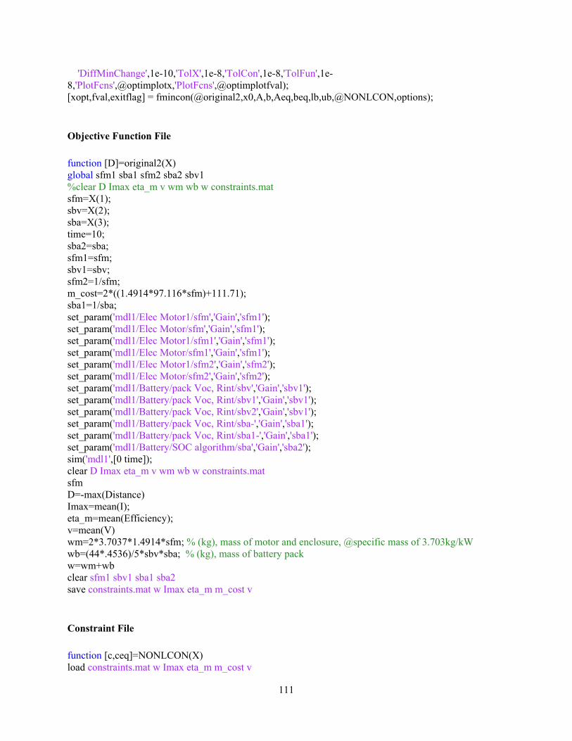
111

'DiffMinChange',1e-10,'TolX',1e-8,'TolCon',1e-8,'TolFun',1e-8,'PlotFcns',@optimplotx,'PlotFcns',@optimplotfval); [xopt,fval,exitflag] = fmincon(@original2,x0,A,b,Aeq,beq,lb,ub,@NONLCON,options);

Objective Function File

function [D]=original2(X) global sfm1 sba1 sfm2 sba2 sbv1 %clear D Imax eta_m v wm wb w constraints.mat sfm=X(1); sbv=X(2); sba=X(3); time=10; sba2=sba; sfm1=sfm; sbv1=sbv; sfm2=1/sfm; m_cost=2*((1.4914*97.116*sfm)+111.71); sba1=1/sba; set_param('mdl1/Elec Motor1/sfm','Gain','sfm1'); set_param('mdl1/Elec Motor/sfm','Gain','sfm1'); set_param('mdl1/Elec Motor1/sfm1','Gain','sfm1'); set_param('mdl1/Elec Motor/sfm1','Gain','sfm1'); set_param('mdl1/Elec Motor1/sfm2','Gain','sfm2'); set_param('mdl1/Elec Motor/sfm2','Gain','sfm2'); set_param('mdl1/Battery/pack Voc, Rint/sbv','Gain','sbv1'); set_param('mdl1/Battery/pack Voc, Rint/sbv1','Gain','sbv1'); set_param('mdl1/Battery/pack Voc, Rint/sbv2','Gain','sbv1'); set_param('mdl1/Battery/pack Voc, Rint/sba-','Gain','sba1'); set_param('mdl1/Battery/pack Voc, Rint/sba1-','Gain','sba1'); set_param('mdl1/Battery/SOC algorithm/sba','Gain','sba2'); sim('mdl1',[0 time]); clear D Imax eta_m v wm wb w constraints.mat sfm D=-max(Distance) Imax=mean(I); eta_m=mean(Efficiency); v=mean(V) wm=2*3.7037*1.4914*sfm; % (kg), mass of motor and enclosure, @specific mass of 3.703kg/kW wb=(44*.4536)/5*sbv*sba; % (kg), mass of battery pack w=wm+wb clear sfm1 sbv1 sba1 sba2 save constraints.mat w Imax eta_m m_cost v

Constraint File

function [c,ceq]=NONLCON(X) load constraints.mat w Imax eta_m m_cost v

112

c=[ w-20; 0.70-eta_m; Imax-50; m_cost-1000; 20-v]; ceq=[];

9.2.2 SIMULINK Blocks

Main Block

Figure 9.1 Main block

6

torque

0.27777

kph_mps

battery

1/0.20

Wheel radius

20

Transmissionratio1

20

Transmissionratio

Terminator

Speed&

Distance

STOP

Stop Simulation

0.5

Splitbetween 2

motors

20

Speed(kph)

Saturation

<=

RelationalOperator

PID

PID Control ler

Motor torque2

Motor torque1

Motor torque

Motor speed rad/s3

Motor speed rad/s2

Motor speed rad/s1

Motor speed rad/s

ElectricMotor

ElectricMotor

Efficiency

Efficiency

0.895

Constant

Battery

Wheelrad/s

Motor rad/s

soc

113

Electric Motror

Figure 9.2 Electric motor block

Battery

Figure 9.3 Battery block

disch

charge

dischargingpower

3

Efficiency

2

net Power>0 discharge

<0 charge

1

motor torqueoutput (Nm)

-K-

sfm2

-K-

sfm1

-K-

sfmmax torque

chargingpower

Sign

Power out is > 0 or < 0 ?

min

MinMax1

0.05s+1

First-order lag

EfficiencyLook-Up

Table (2-D)

|u|

Abs

2

motorspeed (rad/s)

1

Motordemand

Torque (Nm)

power to/f rombattery (W)motor speed

motor speed

torque

1

SOC

PackVoc,Rint

ComputeCurrent

bat

Scope

SOCalgorithm

1

power req'dinto bus (W)

v oc

v oc

soc

soc

Iout

Iout

Power Ef f =v out/v oc

114

PACK Voc, Rint block

Figure 9.4 Pack Voc, Rint block

Current Computation Block

Figure 9.5 Current computation block

2

packresistance

1

pack open-circuit voltage

sbv

sbv2

-K-

sbv1

-K-

sbv

-K-

sba1-

-K-

sba-

Voc

Switch

Scope2

Scope1Scope

Rdis(ohms)

Rchg(ohms)

Product

4

#bty

2

req'd batterypower (W)

1

SOC (prev)

2

V_

1

I_limit current based on max voltage during charge

f(u)

Voc^2-4PreqRint

f(u)

Voc/2Rint

u[2]-u[1]*u[3]

Voc-I*R

Scope7

Scope6

Scope4

Scope2

Scope1

Scope

Psup=I*V

Mux

Mux4

Mux

Mux3

f(u)

Ibty=(Voc-(Voc^2-4RPbty)^.5) -----------------------------

(2*R)

I

Current

< 0

CompareTo Zero

3

Powerrequest (W)

2

Rint

1

Voc

115

SOC Algorithm block

Figure 9.6 SOC algorithm block

Speed and Distance Block

Figure 9.7 Speed and distance block

9.3 Vibrations Subsystem

9.3.1 Methods Comparison

A question might naturally be raised as to why Nomad was used in this optimization problem. A research

was done for different optimization methods and comparison was made for the same starting point :

SOC=(Max Ah capacity-Ah used)/Max Ah capacity

1

SOC1sba2

sba

6

max ah

Scope5

Scope4

Scope3

Scope2

Scope1

SOC

0.1

Gain

1/u

1sxo

Ah used

A-hremaining

0 <= SOC <= 1

1/3600

(sec->hrs)

1

(A)

Drive line + vehicle

Vehicle Speed

Distance

1

Vehicle Speed

1/0.20

1/0.27777

m/s to kmph

0.5*0.7*0.7*1.2

aerodynamic

150

VehicleMass

1s

Scope5 Scope4

Scope3

Scope2

Scope1

Scope0.015*150*9.81

Rolling resistance

1s

u2 Distance

V

1

Wheel Torque

116

Method fmincon DiRect Generic Algorithm Simulated Annealing Nomad

fval 0.5169 0.3489 0.3506 0.3769 0.3508

Improvement -8.07% -37.95% -37.65% -32.97% -37.61%

Running time 90 sec 270 sec 740 sec 340 sec 136 sec

Table 9.1 Methods comparison

Considering the improvement of objective function value and the calculation cost, the running time,

Nomad turns out to be the best.

9.3.2 MATLAB codes

Optimization Execution File

clc clear all clf close all method = 5; % 1: fmincon % 2: generic algorithm % 3: DiRect % 4: Simulated Annealing % 5: fmincon with normalization % Starting Point Sets: % Set 1: x0=[20000;4000;250000;1000;15]; % Set 2: x0=[30000;3000;300000;1500;5]; % Set 3: x0=[23240;3000;200000;1500;5]; % Set 4: x0=[17400;3000;200000;1480;5.4]; lb=[10000;3000;200000;500;5]; ub=[60000;5000;300000;1500;25]; % Nonlinear Optimization Solve: fmincon if method == 1 x0=[17400;3000;200000;1480;5.4]; % options=optimset('Algorithm','active-set','TolX',1e-12,'TolFun',1e-20,'MaxFunEvals',10000,'MaxIter',5000,'DiffMinChange',10^-2,'DiffMaxChange',1); options=optimset('Algorithm','active-set','PlotFcns',@optimplotfval); % [x fval] = fmincon(@transmissibility,x0,[],[],[],[],lb,ub); [x fval] = fmincon(@transmissibility,x0,[],[],[],[],lb,ub,[],options); % [x fval] = fmincon(@transmissibility,x0,A,b,Aeq,beq,lb,ub,@VibSubsCon,options); % A*x <= b % Aeq*x = b elseif method == 2 x0=[20000;4000;250000;1000;15]'; [x fval] = ga(@transmissibility,5,[],[],[],[],lb,ub); elseif method==3

117

% GLOBAL.MaxIter=0; % GLOBAL.MaxEval=1000; GLOBAL=[]; I=[]; nc=0; c_L=[]; c_U=[]; A=[]; b_L=[]; b_U=[]; xopt=gclsolve(@transmissibility,[],lb,ub,A,b_L,b_U,c_L,c_U,I,GLOBAL); elseif method==4 lb=[10000;3000;200000;500;5]'; ub=[30000;5000;300000;1500;25]'; x0=[20000;4000;250000;1000;15]'; [fopt,copt,xopt,numfunc,startpt]=simaneal(@transmissibility,@constr,lb,ub,[],[],x0); elseif method==5 lbWnormalization=lb./ub; ubWnormalization=ub./ub; x0=[20000;4000;250000;1000;15]; x0=x0./ub; options=optimset('Algorithm','active-set','DiffMinChange',10^-3,'PlotFcns',@optimplotfval); f_hist=[]; [x fval] = fmincon(@(x)transmissibilityWnormalization(x,ub),x0,[],[],[],[],lbWnormalization,ubWnormalization,[],options); x=x.*ub; end


function f = transmissibility(x) %% Design Variables %k_S=x(1); %c_S=x(2); %k_T=x(3); %c_T=x(4); %m_T=x(5); %% Parameters m_S=100; g=9.8; F_0=0.1; omega=60; %% Solving ODE [T,Y] = ode45(@(t,y)segwaysuspension2(t,y,x(1),x(2),x(3),x(4),x(5),m_S,g,F_0,omega),[0 5],[0 0 0 0]); %% Calculate objective function

118

human_accel=(x(1)/m_S*(Y(:,3)-Y(:,1))+x(2)/m_S*(Y(:,4)-Y(:,2))-g); ground_accel=-F_0*omega^2*sin(omega*T); f = norm(human_accel)/norm(ground_accel);

Governing Equations for the System (ODEs) File:

function dy = segwaysuspension2(t,y,k_S,c_S,k_T,c_T,m_T,m_S,g,F_0,omega) dy=[0 1 0 0;-k_S/m_S -c_S/m_S k_S/m_S c_S/m_S;0 0 0 1;k_S/m_T c_S/m_T -(k_T+k_S)/m_T -(c_T+c_S)/m_T]*y+[0;-g;0;k_T/m_T*F_0*sin(omega*t)+c_T/m_T*F_0*omega*cos(omega*t)-g];

9.3.3 Nomad Codes


function [fx,cx] = transmissibilityNOMAD(x) %% Design Variables %k_S=x(1); %c_S=x(2); %k_T=x(3); %c_T=x(4); %m_T=x(5); %% Parameters m_S=100; g=9.8; F_0=0.1; omega=60; %% Ground excitation % ft = linspace(0,5,25); % Generate t for f % f = F_0*sin(omega*ft); % Generate f(t) % f1=F_0*omega*cos(omega*ft); %% Solving ODE % [T,Y] = ode45(@(t,y)segwaysuspension(t,y,ft,f1,f,x(1),x(2),x(3),x(4),x(5),m_S,g),[0 5],[0 0 0 0]); [T,Y] = ode45(@(t,y)segwaysuspension2(t,y,x(1),x(2),x(3),x(4),x(5),m_S,g,F_0,omega),[0 5],[0 0 0 0]); %% Calculate objective function human_accel=(x(1)/m_S*(Y(:,3)-Y(:,1))+x(2)/m_S*(Y(:,4)-Y(:,2))-g); ground_accel=-F_0*omega^2*sin(omega*T); fx = norm(human_accel)/norm(ground_accel); cx=[];

119

Initial Points File

function iterate=transmissibilityNOMAD_x0 iterate.x=[20000;4000;250000;1000;15]; iterate.p=; return;

Linear Constraints File

function [A,l,u]=transmissibilityNOMAD_Omega(n) A=eye(n); l=[10000;3000;200000;500;5]; u=[30000;5000;300000;1500;25]; return

9.3.4 Derivation of Governing Equations of the System


The governing equation of the system is based on Newton’s second law, ∑ :

… 9.1

The ground excitation is expressed as:

sin … 9.2

Substitute the ground excitation into the governing system equations, rewriting it as:

120

sin cos… 9.3

Notice that the governing system equation above is of second-order, which cannot be handled by the

famous MATLAB ode45 differential equation solver, simplifications are needed to reduce the order. Set

the state variables to be:

… 9.4

Then:

… 9.5

0 1 0 0

0 0

0 1

0

0 … 9.6

The above equation is of the form where:

0 1 0 0

0 0

0 1 … 9.7

121

0

0 … 9.8

By now the original second-order governing system equation has been reduced to a first-order differential

equation, which can be solved using MATLAB ode45 solver.

9.3.5 Unsuccessful Attempts in the Optimization Process

Changing TolX and TolFun

The previous mathematical model was coded into MATLAB and fmincon was used with ‘active-set’

algorithm and everything else set as default to do the optimization. The ‘active-set’ algorithm was used

because of the warning, ‘Trust-region-reflective method does not currently solve this type of problem,

using active-set (line search) instead’. The starting points were chosen as the center points of the feasible

regions of the design variables. fmincon got stuck in the vicinity of the starting points although several

steps are performed to change its settings:

Step 1: options=optimset('Algorithm','active-set'):

Before After

fval 0.5623 0.5169

k_S 20000 19999.98

c_S 4000 3996.68

k_T 250000 249999.99

c_T 1000 998.94

m_T 5 5.02

Table 9.2 fmincon: results

Optimization terminated: magnitude of directional derivative in search direction less than

2*options.TolFun and maximum constraint violation is less than options.TolCon.

Step 2: options=optimset('Algorithm','active-set','TolFun',1e-10):

Results slightly changed.

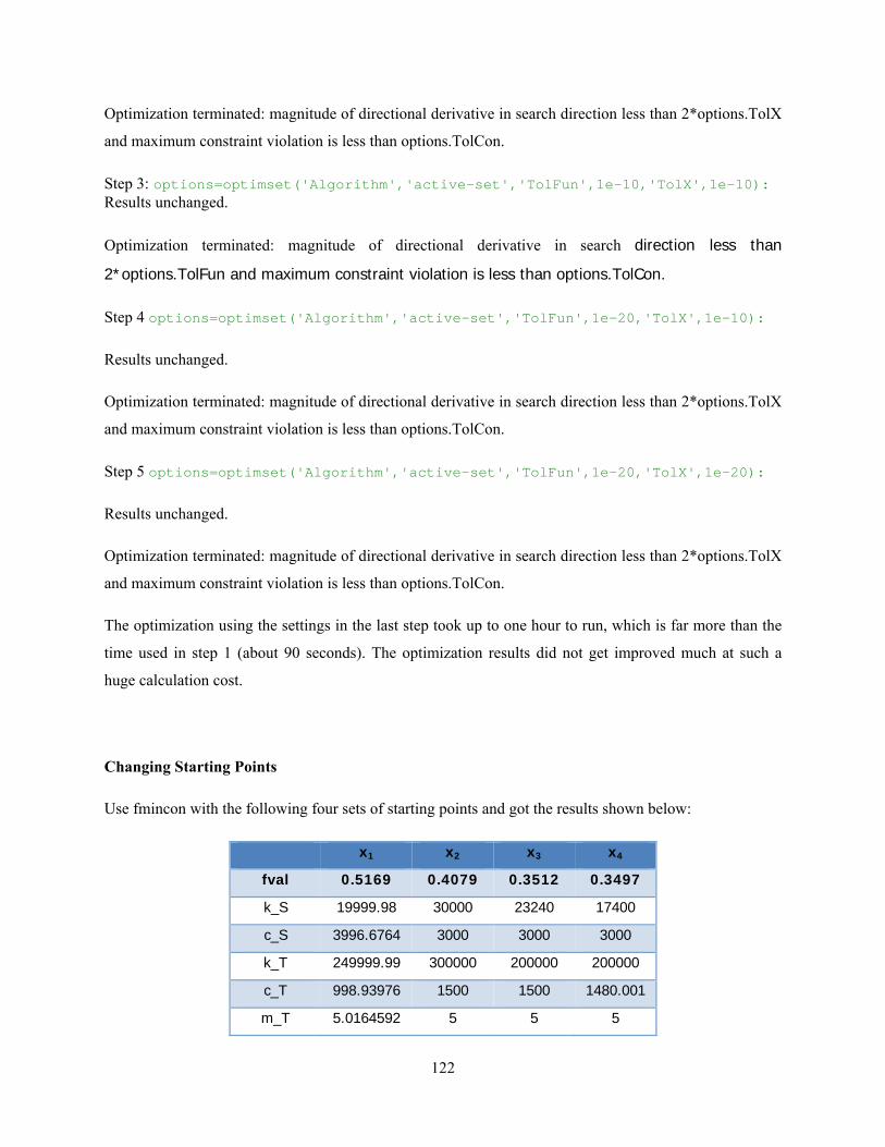
122

Optimization terminated: magnitude of directional derivative in search direction less than 2*options.TolX

and maximum constraint violation is less than options.TolCon.

Step 3: options=optimset('Algorithm','active-set','TolFun',1e-10,'TolX',1e-10): Results unchanged.

Optimization terminated: magnitude of directional derivative in search direction less than

2*options.TolFun and maximum constraint violation is less than options.TolCon.

Step 4 options=optimset('Algorithm','active-set','TolFun',1e-20,'TolX',1e-10):

Results unchanged.



Step 5 options=optimset('Algorithm','active-set','TolFun',1e-20,'TolX',1e-20):

Results unchanged.



The optimization using the settings in the last step took up to one hour to run, which is far more than the

time used in step 1 (about 90 seconds). The optimization results did not get improved much at such a

huge calculation cost.

Changing Starting Points

Use fmincon with the following four sets of starting points and got the results shown below:

x1 x2 x3 x4

fval 0.5169 0.4079 0.3512 0.3497

k_S 19999.98 30000 23240 17400

c_S 3996.6764 3000 3000 3000

k_T 249999.99 300000 200000 200000

c_T 998.93976 1500 1500 1480.001

m_T 5.0164592 5 5 5

123

It can be easily seen that the solution obtained by fmincon still got stuck in the vicinity of all the four sets

starting points. This is due to the global noisy nature of the objective function as can be seen in the

monotonicity analysis.

9.4 Controls Subsystem

9.4.1 Direct Method Codes

Optimization Code

% define parameters M=40; % segway system mass in kg m=120; % passenger mass in kg l=0.7; % lenght of CG along the pendulum in m g=9.81; % acc due to gravity in m/s2 Rw=0.2; % wheel radius in m % plant model matrices A=[0 1 0 0;(M+m)*g/(M*l(i)) 0 0 0;0 0 0 1;-m*g/M 0 0 0]; B=[0;-1/M/l(i);0;1/M]; D=[0]; save plant.mat A B D % define global variables global K Nbar % optimization arguments oA=[]; LB=[1,1,1,1,0.01]; UB=[100;100;100;100;1]; b_L=[]; b_U=[]; c_L=[0;0;1;0;-100]; c_U=[40;25;8;2;-0.0001]; I=[]; GLOBAL.MaxEval=500; GLOBAL.epsilon=1E-4; % call optimization routine Result=gclSolve_new(@PID_matlab, @NONLCON_full, LB, UB, oA, b_L, b_U,c_L, c_U, I, GLOBAL);

124

Constraint Code

function [c,ceq]=NONLCON_full(x) load constraint.mat; c=[os; phi_max; phi_resp; mot_power; E]; ceq=[]; 8.1.3 Plant model function code

function [ts]=PID_matlab(x) global Nbar K load plant.mat q1=x(1); q2=x(2); q3=x(3); q4=x(4); r=x(5); K=lqr(A,B,diag([q1,q2,q3,q4]),r); Nbar=rscale(A,B,[1 1 1 1],D,K); E=eig(A-B*K); set_param('new_model/Nbar','Gain','Nbar'); set_param('new_model/K','Gain','K'); io=getlinio('new_model'); op=operspec('new_model'); op=findop('new_model',op); lin=linearize('new_model',op,io); sys_vel=ss(lin.a,lin.b,lin.c(1,:),lin.d(1,:)); seg_vel=stepinfo(sys_vel); ts=seg_vel.SettlingTime; os=seg_vel.Overshoot; max_vel=20; sys_phi=ss(lin.a,lin.b,lin.c(2,:),lin.d(2,:)); seg_phi=stepinfo(sys_phi); phi_max=seg_phi.Peak; phi_resp=seg_phi.PeakTime; sys_inp=ss(lin.a,lin.b,lin.c(3,:),lin.d(3,:)); seg_inp=stepinfo(sys_inp); force=seg_inp.Peak; mot_power=force*max_vel*(5/18)*(1/1000); % motor power in kw save constraint.mat ts os max_vel phi_max phi_resp mot_power E

125

9.4.2 MATLAB Codes

Optimization Code

% define parameters M=40; % segway system mass in kg m=120; % passenger mass in kg l=0.7; % lenght of CG along the pendulum in m g=9.81; % acc due to gravity in m/s2 Rw=0.2; % wheel radius in m % plant model matrices A=[0 1 0 0;(M+m)*g/(M*l(i)) 0 0 0;0 0 0 1;-m*g/M 0 0 0]; B=[0;-1/M/l(i);0;1/M]; D=[0]; save plant.mat A B D % define global variables global K Nbar % optimization arguments X0=[34.4602;1.3244;99.9925;96.3409;0.0101]; Ao=[]; Bo=[]; Aeq=[]; Beq=[]; LB=[1,1,1,1,0.01]; UB=[100;100;100;100;1]; options = optimset('PlotFcns',@optimplotx,'PlotFcns',@optimplotfval,'MaxIter',500,'MaxFunEvals',1000,'Algorithm','trust-region-reflective'); % call optimization routine [X,FVAL] = FMINCON(@PID_matlab,X0,Ao,Bo,Aeq,Beq,LB,UB,@NONLCON_full,options)

Constraint Code

function [c,ceq]=NONLCON_full(x) load constraint.mat; c=[os-40;phi_max-25;phi_resp-8;-phi_resp+1;mot_power-2;E]; ceq=[];

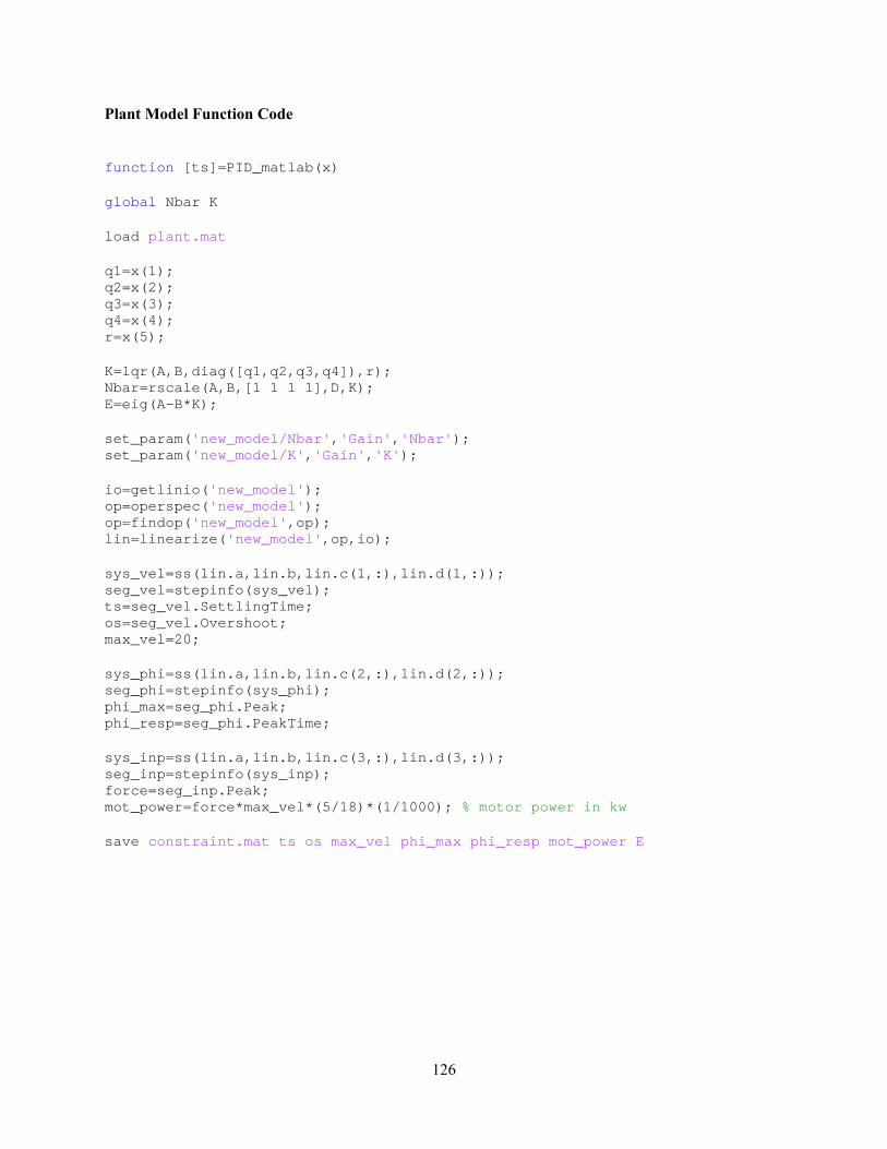
126

Plant Model Function Code

function [ts]=PID_matlab(x) global Nbar K load plant.mat q1=x(1); q2=x(2); q3=x(3); q4=x(4); r=x(5); K=lqr(A,B,diag([q1,q2,q3,q4]),r); Nbar=rscale(A,B,[1 1 1 1],D,K); E=eig(A-B*K); set_param('new_model/Nbar','Gain','Nbar'); set_param('new_model/K','Gain','K'); io=getlinio('new_model'); op=operspec('new_model'); op=findop('new_model',op); lin=linearize('new_model',op,io); sys_vel=ss(lin.a,lin.b,lin.c(1,:),lin.d(1,:)); seg_vel=stepinfo(sys_vel); ts=seg_vel.SettlingTime; os=seg_vel.Overshoot; max_vel=20; sys_phi=ss(lin.a,lin.b,lin.c(2,:),lin.d(2,:)); seg_phi=stepinfo(sys_phi); phi_max=seg_phi.Peak; phi_resp=seg_phi.PeakTime; sys_inp=ss(lin.a,lin.b,lin.c(3,:),lin.d(3,:)); seg_inp=stepinfo(sys_inp); force=seg_inp.Peak; mot_power=force*max_vel*(5/18)*(1/1000); % motor power in kw save constraint.mat ts os max_vel phi_max phi_resp mot_power E

OPTIMAL DESIGN OF A SEGWAY - University of...

Documents

Transcript of OPTIMAL DESIGN OF A SEGWAY - University of...