On the Asymptotic Distribution of (Generalized)

Lorenz Transvariation Measures

Teng Wah Leo∗†

St. Francis Xavier University

20 June, 2017

∗Department of Economics, St. Francis Xavier University. Email Address: tleo@stfx.ca†The author would like to thank Gordon Anderson for his many helpful comments and suggestions in

improving this paper. Nonetheless, all errors remain the author’s.

Abstract

A common problem associated with evaluating dominance relationships between

distribution functions and their moments is the lack of resolution regarding the

direction of dominance as a result of the functions crossing, prevalent in empirical

applications. This paper proposes a method of examining the difference between

(Generalized) Lorenz curves over the entire support of the variables, an idea first

proposed by Anderson and Leo (2017a) and formalized by Anderson et al. (2017)

for the case of stochastic dominance. The method provides a way of ordering all

the (Generalized) Lorenz curves under consideration. The paper also provides the

exact limit distribution of these associated measures, which in consequence of the

results due to Politis and Romano (1994), permits inference via subsampling, in lieu

of the crossing of empirical (Generalized) Lorenz curves. We show that due to the

relationship between the Lorenz curve and the Gini coefficient, the same can be said

of the latter. An example is provided to demonstrate its application.

1 Introduction

There have been significant advances made in the use of stochastic dominance techniques

with the increased use in both the fields of finance and welfare studies. Nonetheless, the

ability of the technique to achieve a complete ordering of distributions under comparison

continues to elude us.1 There has been however significant progress made recently by

Anderson and Leo (2017a). The principal idea reframes the problem of ordering, which

had been to search for the order of dominance that yields a definitive ordering of the

comparisons, to one where the researcher/decision maker chooses the order at which to

examine the order amongst the distributions in question. It uses the entire support, and

measures the difference in area of the distributions against a synthetic best distribution

generated from the hull (lower envelope) created by all the distributions. The idea was

formalized, and asymptotic distribution found in Anderson et al. (2017).

Despite the similarities and relationship between stochastic dominance and Lorenz

dominance (Atkinson (1970) showed that second order stochastic dominance between

two distributions for mean normalized variables is equivalent to Lorenz dominance, while

Shorrocks (1983) showed the same relationship with respect to Generalized Lorenz domi-

nance), there has been little work attempting to solve the issue of establishing a complete

ordering in applications of Lorenz dominance. Some recent work since Beach and David-

son (1983) established the asymptotic distribution of the Lorenz ordinates are Seth and

Yalonetzky (2016), and Zheng (2016), which are closely related to the current work here,

and in Anderson and Leo (2017b).

Zheng (2016) extends the work on Almost Stochastic Dominance by Leshno and Levy

(2002) to Lorenz Dominance by showing, similarly, that by reducing the weight on lower

realization outcomes, a Lorenz dominance relationship may be established, particularly

when Lorenz curves exhibit crossings. Nonetheless, the proposed solution is not fullproof

since frequently the optimal and/or worst states are not separable due to their proximity

to each other. In turn, Seth and Yalonetzky (2016) in seeking to establish whether

a set of bounded qualitative measures achieves convergence or divergence, establishes

the relationship between the induced movements of the measures, and changes in the

Absolute (Generalized) Lorenz ordinates. Both papers are similar to the current paper

here in that they seek to establish the Lorenz dominance relationship, and order the

1Indeed, Atkinson (1970) viewed the partial ordering achieved with Lorenz dominance with skepticism

in lieu of the frequency with which Lorenz curves crossed.

1

different distributions under consideration, developing alternate ways to circumvent the

lack of resolution when Lorenz curves cross. Nonetheless, the proposed solutions are not

fullproof. The method proposed here, and in Anderson and Leo (2017b), and Anderson

et al. (2017) can be extended simply to those methods as well.

The primary contribution of this paper is thus the derivation of the limit distribution

for the measures proposed by Anderson and Leo (2017b), and to provide a subsampling

technique, in lieu of the contact set due to Lorenz curves crossing, thereby allowing

for consistent statistical inference. To consolidate the results, a simple example using

the Current Population Survey drawn from the Integrated Public Use Microdata Series

(IPUMS) is used to examine the evolution of income inequality between 2001 to 2016.

In the following section, we will first establish the definition of the Lorenz Transvari-

ation, extending the idea of Gini Transvariation first proposed by Gini (1916) and Gini

(1959) to comparisons between Lorenz curves, then derive a measure of inequality using

these ideas, and establish their limit distributions. The relationship with the Gini coef-

ficient is also drawn. This is followed by a discussion of the subsampling procedure in

section 3, and section 4 provides a simple example demonstrating the use of the measure,

and method of inference. This is finally followed by the conclusion.

2 Lorenz Transvariation & Related Measures

2.1 Lorenz Transvariation

Let there be M income distributions, Fm, m = {1, 2, . . . ,M}, then for a vector of abscissae

p = [p1, p2, . . . , pK , pK+1 = 1]′, and their corresponding quantiles Y = [Y1, Y2, . . . , YK , YK+1]′,

where YK+1 = Y (pK+1 = 1) = Ymax, the Lorenz curve is just,

L(p) =

∫ p

0

Y (t)

µdF (t) (1)

⇒ L(p) =

∑Nj=1 Y(j)1

(Y(j) ≤ Yp

)∑Nj=1 Y(j)

(2)

2

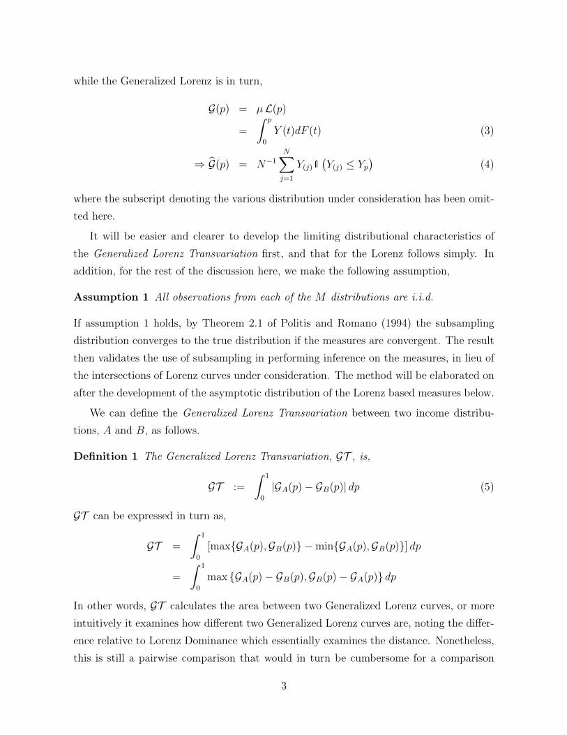
while the Generalized Lorenz is in turn,

G(p) = µL(p)

=

∫ p

0

Y (t)dF (t) (3)

⇒ G(p) = N−1

N∑j=1

Y(j)1(Y(j) ≤ Yp

)(4)

where the subscript denoting the various distribution under consideration has been omit-

ted here.

It will be easier and clearer to develop the limiting distributional characteristics of

the Generalized Lorenz Transvariation first, and that for the Lorenz follows simply. In

addition, for the rest of the discussion here, we make the following assumption,

Assumption 1 All observations from each of the M distributions are i.i.d.

If assumption 1 holds, by Theorem 2.1 of Politis and Romano (1994) the subsampling

distribution converges to the true distribution if the measures are convergent. The result

then validates the use of subsampling in performing inference on the measures, in lieu of

the intersections of Lorenz curves under consideration. The method will be elaborated on

after the development of the asymptotic distribution of the Lorenz based measures below.

We can define the Generalized Lorenz Transvariation between two income distribu-

tions, A and B, as follows.

Definition 1 The Generalized Lorenz Transvariation, GT , is,

GT :=

∫ 1

0

|GA(p)− GB(p)| dp (5)

GT can be expressed in turn as,

GT =

∫ 1

0

[max{GA(p),GB(p)} −min{GA(p),GB(p)}] dp

=

∫ 1

0

max {GA(p)− GB(p),GB(p)− GA(p)} dp

In other words, GT calculates the area between two Generalized Lorenz curves, or more

intuitively it examines how different two Generalized Lorenz curves are, noting the differ-

ence relative to Lorenz Dominance which essentially examines the distance. Nonetheless,

this is still a pairwise comparison that would in turn be cumbersome for a comparison

3

set composed of large number of distributions. More succinctly, since there is no common

basis of comparison, pairwise comparisons when there are large number of distributions

under consideration will unlikely yield a complete order, not to mention the large number

of permutations of comparisons that need to be exhausted.

To examine the asymptotic characteristics of the estimator among the M Generalized

Lorenz curves under consideration, define

Pk = {p ∈ P : Gk(p) > Gk′(p) ,∀k′ 6= k}

Pk=k′ = {p ∈ P : Gk(p) = Gk′(p) ,∀k′ 6= k}

where m,m′ = {1, . . . ,M} = Q. We will assume that Pk=k′ has Lebesgue measure of zero,

so that there are no range of the ordinates where the Lorenz curves under consideration

are the same. Further, we will assume for simplicity here that the same sample size is

drawn from each i.i.d. distribution, N .

In addition, define,

Gm(p) = N−1

N∑j=1

Y m(j)1

(Y m

(j) ≤ Y (p))

Gm(pk ∧ pk′) = N−1

N∑i=1

N∑j=1

Y m(i)Y

m(j)1

(Y m

(i) ≤ Y (pk ∧ pk′), Y m(j) ≤ Y (pk ∧ pk′)

)

Lm(p) =N−1

∑Nj=1 Y

m(j)1

(Y m

(j) ≤ Y (p))

µm

µm = N−1

N∑j=1

Y m(j)

Sqm,m′,j =

∫Pq

[Y m

(j)1(Y m

(j) ≤ Y (p))− Y m′

(j) 1

(Y m′

(j) ≤ Y (p))]dp

Km,q,j =M∑q=1

∫Pq

[Y q

(j)1

(Y q

(j) ≤ Y (p))− Y m

(j)1(Y m

(j) ≤ Y (p))]dp =

M∑q=1

Sqq,m,j

The following result extends the work by Anderson et al. (2017) and establishes the

asymptotic distribution of the Generalized Lorenz Transvariation.

Theorem 1 For m 6= m′ ∈ Q, the Generalized Lorenz Transvariation , GT , is asymp-

4

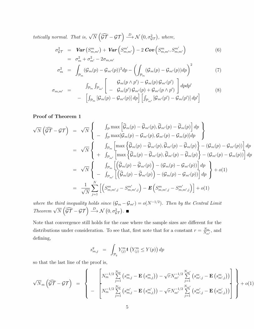
totically normal. That is,√N(GT − GT

)D−→ N

(0, σ2

GT), where,

σ2GT = Var

(Smm,m′

)+ Var

(Sm

′

m,m′

)− 2Cov

(Smm,m′ , Sm

′

m,m′

)(6)

= σ2m + σ2

m′ − 2σm,m′

σ2m =

∫Pm

(Gm(p)− Gm′(p))2dp−(∫Pm

(Gm(p)− Gm′(p))dp

)2

(7)

σm,m′ =

∫Pm

∫Pm′

[Gm(p ∧ p′)− Gm(p)Gm′(p′)

− Gm(p′)Gm′(p) + Gm′(p ∧ p′)

]dpdp′

−[∫Pm [Gm(p)− Gm′(p)] dp

] [∫Pm′

[Gm′(p′)− Gm(p′)] dp′] (8)

Proof of Theorem 1

√N(GT − GT

)=√N

∫P max

[Gm(p)− Gm′(p), Gm′(p)− Gm(p)

]dp

−∫P max[Gm(p)− Gm′(p),Gm′(p)− Gm(p)]dp

=√N

∫Pm

[max

{Gm(p)− Gm′(p), Gm′(p)− Gm(p)

}− (Gm(p)− Gm′(p))

]dp

+∫Pm′

[max

{Gm(p)− Gm′(p), Gm′(p)− Gm(p)

}− (Gm′(p)− Gm(p))

]dp

=√N

∫Pm

[(Gm(p)− Gm′(p)

)− (Gm(p)− Gm′(p))

]dp

−∫Pm′

[(Gm(p)− Gm′(p)

)− (Gm(p)− Gm′(p))

]dp

+ o(1)

=1√N

N∑j=1

[(Smm,m′,j − Sm

′

m,m′,j

)−E

(Smm,m′,j − Sm

′

m,m′,j

)]+ o(1)

where the third inequality holds since (Gm−Gm′) = o(N−1/2). Then by the Central Limit

Theorem√N(GT − GT

)D−→ N

(0, σ2

GT).

Note that convergence still holds for the case where the sample sizes are different for the

distributions under consideration. To see that, first note that for a constant r = NmNm′

, and

defining,

sqm,j =

∫PqY m

(j)1(Y m

(j) ≤ Y (p))dp

so that the last line of the proof is,

√Nm

(GT − GT

)=

[N−1/2m

Nm∑j=1

(smm,j − E

(smm,j

))−√rN−1/2m′

Nm′∑j=1

(smm′,j − E

(smm′,j

))]

−

[N−1/2m

Nm∑j=1

(sm

′m,j − E

(sm

′m,j

))−√rN−1/2m′

Nm′∑j=1

(sm

′

m′,j − E(sm

′

m′,j

))]+ o(1)

5

and as in the above proof, by the Central Limit Theorem√Nm

(GT − GT

)D−→ N

(0, σ2

GT),

where σ2GT is a function of r. The critical point here being the fact that the measure will

continue to be convergent, validating the use of the subsampling procedure proposed by

Politis and Romano (1994) and Politis et al. (1999).

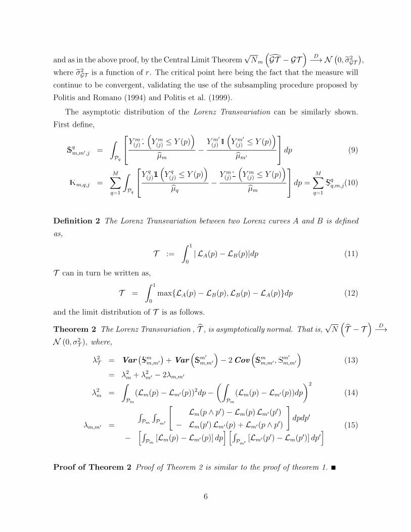
The asymptotic distribution of the Lorenz Transvariation can be similarly shown.

First define,

Sqm,m′,j =

∫Pq

Y m(j)1

(Y m

(j) ≤ Y (p))

µm−Y m′

(j) 1

(Y m′

(j) ≤ Y (p))

µm′

dp (9)

Km,q,j =M∑q=1

∫Pq

Y q(j)1

(Y q

(j) ≤ Y (p))

µq−Y m

(j)1

(Y m

(j) ≤ Y (p))

µm

dp =M∑q=1

Sqq,m,j(10)

Definition 2 The Lorenz Transvariation between two Lorenz curves A and B is defined

as,

T :=

∫ 1

0

| LA(p)− LB(p)|dp (11)

T can in turn be written as,

T =

∫ 1

0

max{LA(p)− LB(p),LB(p)− LA(p)}dp (12)

and the limit distribution of T is as follows.

Theorem 2 The Lorenz Transvariation , T , is asymptotically normal. That is,√N(T − T

)D−→

N (0, σ2T ), where,

λ2T = Var

(Smm,m′

)+ Var

(Sm′

m,m′

)− 2Cov

(Smm,m′ ,Sm

′

m,m′

)(13)

= λ2m + λ2

m′ − 2λm,m′

λ2m =

∫Pm

(Lm(p)− Lm′(p))2dp−(∫Pm

(Lm(p)− Lm′(p))dp

)2

(14)

λm,m′ =

∫Pm

∫Pm′

[Lm(p ∧ p′)− Lm(p)Lm′(p′)

− Lm(p′)Lm′(p) + Lm′(p ∧ p′)

]dpdp′

−[∫Pm [Lm(p)− Lm′(p)] dp

] [∫Pm′

[Lm′(p′)− Lm(p′)] dp′] (15)

Proof of Theorem 2 Proof of Theorem 2 is similar to the proof of theorem 1.

6

2.2 Relative Potential Lorenz Transvariation

However, the Generalized Lorenz Transvariation and the Lorenz Transvariation do not

permit a complete ranking of the Lorenz curves under consideration since they are just

pairwise comparisons, nor is GT or T ∈ [0, 1]. In other words, there is no common basis

against which all the Lorenz curves are compared, so that a consistent ordering can be

achieved. What is needed is such a common base of comparison. To that end, this can be

achieved by creating synthetically an upper envelope consisting of piecewise combinations

of all the Generalized Lorenz curves under consideration. Then the transvariation measure

of any Generalized Lorenz m ∈ Q is the Potential Generalized Lorenz Transvariation, and

it will provide a consistent ordering.

To understand the measure, first denote the upper envelope generated by max∪Mm=1 Lm{G(p)} =

G(p), then denote G(p) as the synthetic baseline against which all the Generalized Lorenz

curves are compared against. Precisely,

Definition 3 The Potential Generalized Lorenz Transvariation is defined as the area be-

tween the synthetic empirical best case scenario represented by G(p), and the mth gener-

alized Lorenz curve,

GBm :=

∫P

[maxq∈Q{Gq(p)} − Gm(p)

]dp (16)

=

∫P

[maxq∈Q{Gq(p)− Gm(p)}

]dp

=

∫P

[G(p)− Gm(p)

]dp

The following theorem shows that GBm for m = 1, . . . ,M is asymptotically normal.

Theorem 3 The Potential Generalized Lorenz Transvariation, GBm, is asymptotically

normal. That is,√N(GBm − GBm

)D−→ N

(0, σ2

GBm

), where σ2

GBm is,

σ2GBm =

M∑q=1

Var(Sqq,m

)− 2

M∑q=1

M∑q′ 6=q

Cov(Sqq,m, S

q′

q′,m

)=

M∑q=1

σ2q − 2

M∑q=1

M∑q′ 6=q

σq,q′ (17)

7

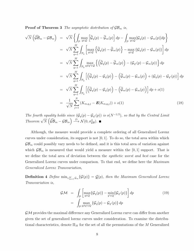
Proof of Theorem 3 The asymptotic distribution of GBm is,

√N(GBm − GBm

)=√N

{∫P

maxq∈Q

[Gq(p)− Gm(p)

]dp−

∫P

maxq∈Q

[Gq(p)− Gm(p)]dp

}=√N

M∑q=1

∫Pq

[maxq∈Q

{Gq(p)− Gm(p)

}−max

q∈Q{Gq(p)− Gm(p)}

]dp

=√N

M∑q=1

∫Pq

maxq 6=q′∈Q

{(Gq(p)− Gm(p)

)− (Gq′(p)− Gm(p))

}dp

=√N

M∑q=1

∫Pq

[(Gq(p)− Gq(p)

)−(Gm(p)− Gm(p)

)+ (Gq(p)− Gq′(p))

]dp

=√N

M∑q=1

∫Pq

[(Gq(p)− Gq(p)

)−(Gm(p)− Gm(p)

)]dp+ o(1)

=1√N

N∑j=1

(Km,q,j −E(Km,q,j)) + o(1) (18)

The fourth equality holds since (Gq(p)− Gq′(p)) is o(N−1/2), so that by the Central Limit

Theorem√N(GBm − GBm

)D−→ N (0, σ2

GB).

Although, the measure would provide a complete ordering of all Generalized Lorenz

curves under consideration, its support is not [0, 1]. To do so, the total area within which

GBm could possibly vary needs to be defined, and it is this total area of variation against

which GBm is measured that would yield a measure within the [0, 1] support. That is

we define the total area of deviation between the synthetic worst and best case for the

Generalized Lorenz curves under comparison. To that end, we define here the Maximum

Generalized Lorenz Transvariation,

Definition 4 Define min∪Mm=1 Gm{G(p)} = G(p), then the Maximum Generalized Lorenz

Transvariation is,

GM =

∫P

[maxq∈Q{Gq(p)} −min

q′∈Q{Gq′(p)}

]dp (19)

=

∫P

maxq 6=q′∈Q

{Gq(p)− Gq′(p)} dp

GM provides the maximal difference any Generalized Lorenz curve can differ from another

given the set of generalized lorenz curves under consideration. To examine the distribu-

tional characteristics, denote ΠM for the set of all the permutations of the M Generalized

8

Lorenz curves, where a typical vector denoted by π = [π1, π2, . . . , πM ]′ ∈ ΠM , πm = π(m),

m ∈ Q, such that Pm = ∪{π:πM=m}Γπ, where Γπ = {p ∈ P : Gπ1(p) < Gπ2(p) < . . .GπM (p)}.In other words the union of all the permutations where max

j∈Q{Gj(p)} = Gm(p). To be clear,

πm then is a catchment of the M distributions under consideration that is the mth highest.

Then combining both the measures of equations (16) and (19) we can define the

Relative Potential Generalized Lorenz Transvariation.

Definition 5 The Relative Potential Generalized Lorenz Transvariation is

GRm =

∫P [maxq∈Q {Gq(p)− Gm(p)}] dp∫P maxq 6=q′∈Q {Gq(p)− Gq′(p)} dp

(20)

and it has a support of [0, 1].

An inequality measure using GRm can be thus defined:

Definition 6 The Relative Potential Generalized Lorenz Transvariation Inequality Mea-

sure is,

GIm = 1−∫P [maxq∈Q {Gq(p)− Gm(p)}] dp∫P maxq 6=q′∈Q {Gq(p)− Gq′(p)} dp

= 1− GRm (21)

and GIm ∈ [0, 1].

Thus for Generalized Lorenz curve m ∈ Q which is closest to the upper envelope would

have GIm closest to 1, and implies that the underlying population exhibits the lowest level

of income inequality. On the other hand, for m′ ∈ Q, m 6= m′, which is furthest away

from the upper envelope, and in consequence, closest to the lower hull would have GIm′

close to 0, and exhibits the highest level of income inequality among the M populations

under consideration.

Evaluating GIm for all M Generalized Lorenz curves under consideration would yield

a complete ranking of differential in income inequality. Further, given the asymptotic dis-

tribution, inference on these measures are easily performed. However, this is complicated

by the crossing of Generalized Lorenz curves in empirical applications, which requires the

estimation of this intersection points, or alternately using subsampling methods. Since

subsampling as proposed by Politis and Romano (1994) and Politis et al. (1999) requires

only that the statistic be convergent, the technique is adopted here and the following

section will discuss this technique in greater detail.

9

To determine the asymptotic distribution of GIm define now,

Γπ = {p ∈ P : Gπ1(p) < Gπ2(p) < . . .GπM (p)} (22)

Aj =∑π∈ΠM

∫Γπ

[Y πM

(j) 1

(Y πM

(j) ≤ Y (p))− Y π1

(j)1

(Y π1

(j) ≤ Y (p))]dp (23)

Theorem 4 The Relative Potential Generalized Lorenz Transvariation, GRm, is asymp-

totically normal. That is,√N(GRm − GRm

)D−→ N

(0,∆′G,mσ

2GBm∆G,m

), where σ2

GBm is

as defined in theorem 3, and

∆G,m =

[1GM

− GBmGM2

](24)

so that√N(GIm − GIm

)D−→ N

(0,∆′G,mσ

2GBm∆G,m

).

Proof of Theorem 4 Note that,

√N(GM− GM

)=√N

∫P

[maxq 6=q′∈Q

{Gq(p)− Gq′(p)

}− max

q 6=q′∈Q{Gq(p)− Gq′(p)}

]dp

=√N∑π∈ΠM

∫Γπ

[maxq 6=q′∈Q

{Gq(p)− Gq′(p)

}− max

q 6=q′∈Q{Gq(p)− Gq′(p)}

]dp

=√N∑π∈ΠM

∫Γπ

[maxq 6=q′∈Q

{Gq(p)− Gq′(p)

}− (GπM (p)− Gπ1(p))

]dp

=√N∑π∈ΠM

∫Γπ

[maxq 6=q′∈Q

{GπM (p)− Gπ1(p)

}− (GπM (p)− Gπ1(p))

]dp+ o(1)

=1√N

N∑j=1

(Aj −E (Aj)) + o(1) (25)

Then by the results from theorem 3, and using the Delta Method,(GRm − GRm

)=

(GBmGM

− GBmGM

)→ N

(0,∆′G,mσ

2GBm∆G,m

)for m = {1, . . . ,M}, and the rest of the theorem follows.

The same idea can be applied to the Lorenz Transvariation, the proofs of which are

similar, augmented by the following definition:

10

Definition 7 The Potential Lorenz Transvariation is defined as the area between the

synthetic empirical best case scenario represented by L(p), and the mth Lorenz curve,

Bm :=

∫P

[maxq∈Q{Lq(p)} − Lm(p)

]dp (26)

=

∫P

[maxq∈Q{Lq(p)− Lm(p)}

]dp

=

∫P

[L(p)− Lm(p)

]dp

Theorem 5 The Potential Lorenz Transvariation, Bm, is asymptotically normal. That

is,√N(Bm − Bm

)D−→ N

(0, σ2

Bm

), where σ2

Bm is,

λ2Bm =

M∑q=1

Var(Sqq,m

)− 2

M∑q=1

M∑q′ 6=q

Cov(Sqq,m,S

q′

q′,m

)=

M∑q=1

λ2q − 2

M∑q=1

M∑q′ 6=q

λq,q′ (27)

Proof of Theorem 5 Proof of Theorem 5 is similar to the proof of theorem 3.

Then an inequality measure based on the Lorenz curve needs the following definitions

for the Maximum Lorenz Transvariation, and the Relative Potential Lorenz Transvaria-

tion.

Definition 8 Define min∪Mm=1 Lm{L(p)} = L(p), then the Maximum Lorenz Transvaria-

tion is,

M =

∫P

[maxq∈Q{Lq(p)} −min

q′∈Q{Lq′(p)}

]dp (28)

=

∫P

maxq 6=q′∈Q

{Lq(p)− Lq′(p)} dp

Then combining both the measures of equations (26) and (28) we can define the

Relative Potential Generalized Lorenz Transvariation.

Definition 9 The Relative Potential Generalized Lorenz Transvariation is

Rm =

∫P [maxq∈Q {Lq(p)− Lm(p)}] dp∫P maxq 6=q′∈Q {Lq(p)− Lq′(p)} dp

(29)

and it has a support of [0, 1].

11

The inequality measure based on the Lorenz curve using Rm can be thus defined:

Definition 10 The Relative Potential Lorenz Transvariation Inequality Measure is,

Im = 1−∫P [maxq∈Q {Lq(p)− Lm(p)}] dp∫P maxq 6=q′∈Q {Lq(p)− Lq′(p)} dp

= 1−Rm (30)

and Im ∈ [0, 1].

Let ΨM denote the set of all the permutations of the M Lorenz curves, where the

typical vector is ψ = [ψ1, ψ2, . . . , ψM ]′ ∈ ΨM , such that Pm = ∪ψ:ψM=mΘψ, where

Θψ = {p ∈ P : Lψ1(p) < Lψ2(p) < . . .LψM (p)} (31)

Aj =∑ψ∈ΨM

∫Θπ

Y ψM(j) 1

(Y ψM

(j) ≤ Y (p))

µψM−Y ψ1

(j) 1

(Y ψ1

(j) ≤ Y (p))

µψ1

dp (32)

Theorem 6 The Relative Potential Lorenz Transvariation, Rm, is asymptotically nor-

mal. That is,√N(Rm −Rm

)D−→ N

(0,∆′L,mσ

2B∆L,m

), where σ2

B is as defined in theo-

rem 3, and

∆L,m =

[1Mm

− BmM2m

](33)

so that√N(Im − Im

)D−→ N

(0,∆′L,mσ

2B∆L,m

).

Proof of Theorem 6 Proof of theorem 6 is similar to the proof of theorem 4.

2.3 Relationship of Lorenz Transvariation to Gini

Observe that since the Gini coefficient may be written as,

G ≡ G(L) =

∫ 1

0[p− L(p)]dp∫ 1

0pdp

12

we can think of measuring the distance between the Lorenz curves with respect to the 45◦

line instead of L in the development of the transvariation measures. Specifically, we can

write Bm, Rm, and M as,

Bm =

∫P

[L(p)− Lm(p)

]dp

=

∫P

{[p− Lm(p)]− [p− L(p)]

}dp∫ 1

0pdp

= G(Lm)−G(L)

(34)

and

M = G (L)−G(L)

(35)

so that Rm is,

Rm =G(Lm)−G

(L)

G (L)−G(L) (36)

and Im can be similarly written.

This suggests that the same inequality measure discussed thus far can be expressed in

terms of the Gini coefficient. First note that,

max∪Mm=1

Gm ≡ G = max∪Mm=1

{∫ 1

0[p− Lm(p)]dp∫ 1

0pdp

}

≤∫P [p− L(p)] dp∫ 1

0pdp

:= G(L)

where the last equality follows since,∫P

[p− L(p)] dp ≥ max∪Mm=1

{∫ 1

0

[p− Lm(p)]dp

}because L ≤ Lm(p) for all p, m = {1, . . . ,M}. By a similar argument, min∪Mm=1

Gm =

G ≥ G(L). Then we can define parallel concepts of Potential, Maximum, and Relative

Transvariation in terms of the Gini coefficient as,

B = G−G (37)

M = G−G (38)

R =G−G

G−G(39)

13

where G := G(L), and the formulae are for the Potential Gini Transvariation, Maximum

Gini Transvariation, and Relative Gini Transvariation respectively. Note further that

R ∈ [0, 1]. Next, observe that since,

G (L)−G(L)≥ G−G

and G−G(L)≥ G−G

we can bound the Relative Gini Transvariation. First, define,

G(L)−G = ∆ ≥ 0

G(L)−G = ∆ ≤ 0

∆−∆ = ∆ ≥ 0

Then,

Rm =

∫ 10 [p−Lm(p)]dp∫ 1

0 pdp−G

G−G

=

∫ 10 [p−Lm(p)]dp∫ 1

0 pdp−G(L) + ∆

G(L)−G(L)−∆

≥

∫ 10 [p−Lm(p)]dp∫ 1

0 pdp−G(L)

G(L)−G(L)= Rm

Further, since

G = G(L) = G(L)

then

1 = R ≥ R

In other words, the upper bound of the Relative Gini Transvariation is higher than the

14

upper bound of the Relative Lorenz Transvariation. Similarly for the lower bound,

R = R(L) =

∫P [p−L]dp∫ 1

0 pdp−G(L)

G(L)−G(L)

≥

∫P [p−L]dp∫ 1

0 pdp−G(L) + ∆

G(L)−G(L)−∆

=

∫P [p−L]dp∫ 1

0 pdp−G

G−G

=

min∪Mm=1{∫P [p−L]dp}∫ 10 pdp

−G

G−G= R = 0

Finally, an appropriate inequality measure with respect to the Relative Gini Transvaria-

tion would be,

Im = 1−G(Lm) (40)

Insofar as the Gini Transvariation can be written in terms of the Lorenz curve, the

prior proofs of convergence can be adapted for that purpose. Further, in lieu of the compli-

cations due to intersections between Lorenz curves under consideration, the subsampling

method may be adapted here as well for inference. A full discussion is omitted here as it

is outside the scope of the current paper.

3 Estimation & Inference

The Lorenz Transvariation, Maximal Lorenz Transvariation, and Relative Potential Lorenz

Transvariation and their Generalized counterparts can be estimated by recognizing the

the integrals over the indicator functions are essentially step functions over the chosen

quantiles, so that the transvariation measures are differences between these steps.

The intersection points can be appropriately estimated to minimize power loss via

subsampling techniques as prescribed by Politis and Romano (1994), and extended and

summarized in Politis et al. (1999). On a related procedure to stochastic dominance, see

Linton et al. (2005) and Linton et al. (2014). The steps are,

1. For each of the populations under consideraion, obtain the relevant statistics of GIor I using the full sample, WN := {Yj : j = 1, . . . , N}.

15

2. Generate subsamples of length b, Wn,b := {Yn, . . . , Yn+b−1} for n = 1, . . . , n− b+ 1.

3. Calculate the relevant statistics GIn,b or In,b, using the subsamples Wn,b.

4. The sampling distribution of√N(GI − GI

)or√N(I − I

), is approximated by,

ΦN,b(ω) =1

N − b+ 1

N−b+1∑n=1

1

(√b(GIn,b − GI

)≤ ω

)(41)

ΨN,b(ω) =1

N − b+ 1

N−b+1∑n=1

1

(√b(In,b − I

)≤ ω

)(42)

respectively.

5. Find the requisite αth sample quantile of ΦN,b(ω) or ΨN,b(ω),

φN,b(α) := inf{ω : ΦN,b(ω) ≥ α} (43)

ψN,b(α) := inf{ω : ΨN,b(ω) ≥ α} (44)

respectively.

6. The confidence interval for GI or I can be calculated using the respective formulae:

CIφN,b :=[GI −N−1/2φN,b

(1− α

2

), GI −N−1/2φN,b

(α2

)](45)

CIψN,b :=[I −N−1/2ψN,b

(1− α

2

), I −N−1/2ψN,b

(α2

)](46)

Following Politis and Romano (1994), the following Theorem shows that the confidence

interval has an asymptotically correct coverage.

Theorem 7 Given assumption 1 is true, then if b→∞ and bN→ 0, then

Pr(GI ∈ CIφN,b) → (1− α) as N →∞

Pr(I ∈ CIψN,b) → (1− α) as N →∞

Proof of Theorem 7 Given that the data is i.i.d., and the convergence of the transvaria-

tion measures discussed, the proof follows directly from theorem 2.1 of Politis and Romano

(1994)

16

There remains the second order concern of the choice of the subsample size b, of

which some guidance is provided in Politis and Romano (1994), and Linton et al. (2005).

Although for the example in the following section, we used only a single subsample size

where b = Nln(ln(N))

, Linton et al. (2005) provides some guidance on automating the process

for inference. Linton et al. (2005) proposed the calculation of the mean and median critical

values, and/or p-values of the measure. First denote

BN =[bN1 < bN2 < · · · < bNrN

]as the sequence of subsample sizes, where bNj < N are integers, and rN is the number

of elements in BN . The choice of the subsample size are then integer values between

ln(ln(N)) and Nln(ln(N))

. These subsample sizes can be applied consistently for all the

Lorenz curves under comparison. In turn, the mean and median choice for the statistic

for inference are used. For instance, suppose the null hypothesis is for H0 : GI = 1 or

H0 : I = 1. Then from the appropriately generated sampling distribution under H0,

denote the sample quantitle as φ1N,bNi

(ω) and ψ1N,bNi

(ω) respectively for GI and I. Denote

the critical values for each subsample i, i = {1, . . . , rN}, CφN,bNi (1− α) and CψN,bNi (1− α),

for the Generalized Lorenz and Lorenz based inequality measures respectively. Then the

decision is based on the mean and median values of the critical values at α respectively,

CφN(1− α) =1

rN

rN∑i=1

CφN,bNi (1− α) (47)

Cφ,MedianN (1− α) = median{CφN,bNi (1− α) : i = 1, . . . , rN} (48)

and

CψN(1− α) =1

rN

rN∑i=1

CψN,bNi (1− α) (49)

Cψ,MedianN (1− α) = median{CψN,bNi (1− α) : i = 1, . . . , rN} (50)

where the mean critical value/criterion is equivalent to basing inference on the average

opinion, while the latter is the majority opinion. In the case on hand, the researcher

rejects the null if GI < CφN(1− α), or GI < Cφ,MedianN (1− α).

17

4 An Example

We demonstrate here the use of the Relative Potential Lorenz Transvariation in providing

a complete ordering, as well as the use of the subsampling technique for inference, using

U.S. Current Population Survey drawn from the Integrated Public Use Microdata Series

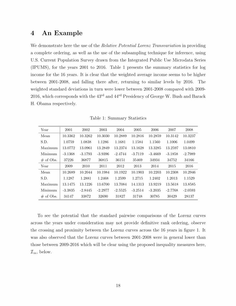
(IPUMS), for the years 2001 to 2016. Table 1 presents the summary statistics for log

income for the 16 years. It is clear that the weighted average income seems to be higher

between 2001-2008, and falling there after, returning to similar levels by 2016. The

weighted standard deviations in turn were lower between 2001-2008 compared with 2009-

2016, which corresponds with the 43rd and 44rd Presidency of George W. Bush and Barack

H. Obama respectively.

Table 1: Summary Statistics

Year 2001 2002 2003 2004 2005 2006 2007 2008

Mean 10.3362 10.3262 10.3030 10.2889 10.2816 10.2859 10.3142 10.3237

S.D. 1.0759 1.0838 1.1286 1.1681 1.1584 1.1560 1.1006 1.0499

Maximum 13.0772 13.0961 13.2849 13.2374 13.1628 13.3285 13.2597 13.0810

Minimum -3.1368 -3.1793 -3.9396 -2.4744 -3.7119 -3.4669 -3.1858 -2.7989

# of Obs. 37226 36877 36815 36151 35469 34934 34752 34166

Year 2009 2010 2011 2012 2013 2014 2015 2016

Mean 10.2689 10.2044 10.1984 10.1922 10.1903 10.2203 10.2308 10.2946

S.D. 1.1287 1.2881 1.2468 1.2599 1.2715 1.2402 1.2013 1.1529

Maximum 13.1475 13.1226 13.6700 13.7084 14.1313 13.9219 13.5618 13.8585

Minimum -3.3835 -2.8445 -2.2977 -2.5525 -3.2514 -3.2035 -2.7768 -2.0593

# of Obs. 34147 33872 32690 31827 31748 30785 30429 28137

To see the potential that the standard pairwise comparisons of the Lorenz curves

across the years under consideration may not provide definitive rank ordering, observe

the crossing and proximity between the Lorenz curves across the 16 years in figure 1. It

was also observed that the Lorenz curves between 2001-2008 were in general lower than

those between 2009-2016 which will be clear using the proposed inequality measures here,

Im, below.

18

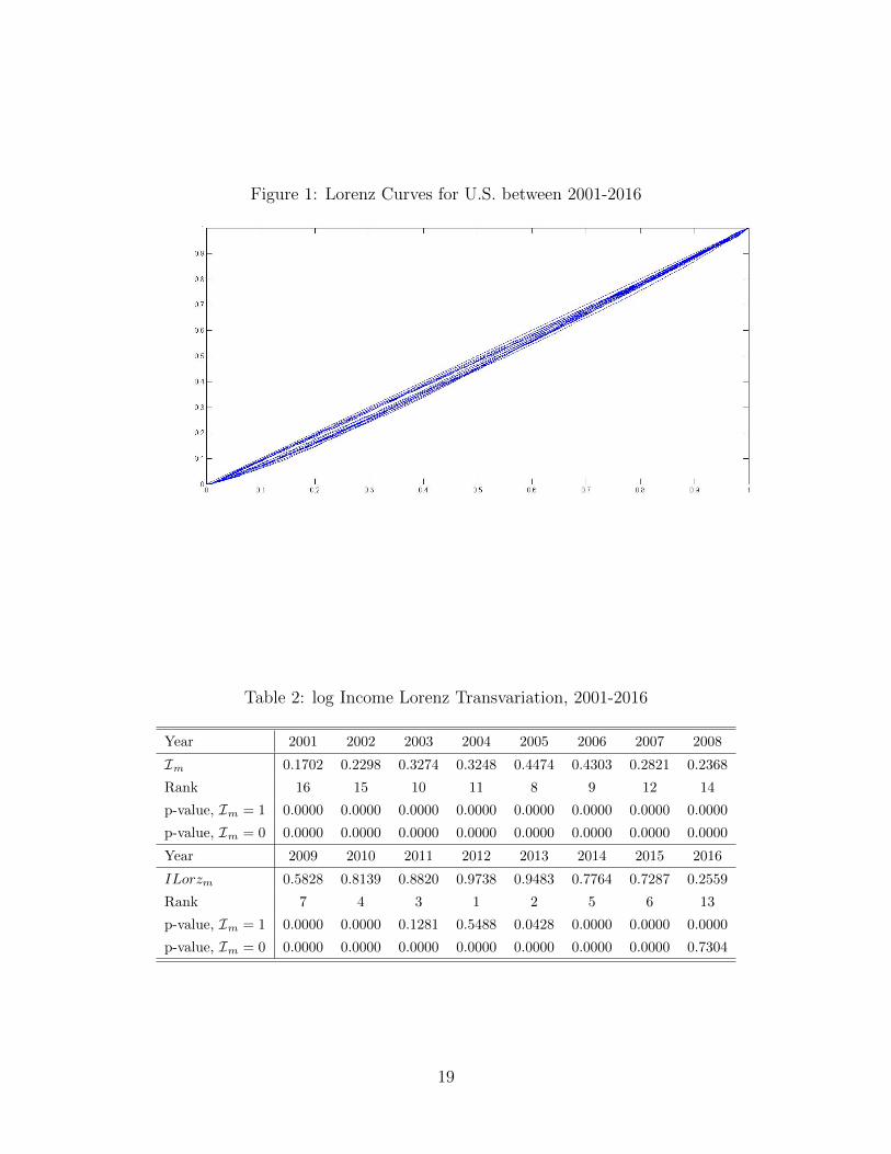
Figure 1: Lorenz Curves for U.S. between 2001-2016

Table 2: log Income Lorenz Transvariation, 2001-2016

Year 2001 2002 2003 2004 2005 2006 2007 2008

Im 0.1702 0.2298 0.3274 0.3248 0.4474 0.4303 0.2821 0.2368

Rank 16 15 10 11 8 9 12 14

p-value, Im = 1 0.0000 0.0000 0.0000 0.0000 0.0000 0.0000 0.0000 0.0000

p-value, Im = 0 0.0000 0.0000 0.0000 0.0000 0.0000 0.0000 0.0000 0.0000

Year 2009 2010 2011 2012 2013 2014 2015 2016

ILorzm 0.5828 0.8139 0.8820 0.9738 0.9483 0.7764 0.7287 0.2559

Rank 7 4 3 1 2 5 6 13

p-value, Im = 1 0.0000 0.0000 0.1281 0.5488 0.0428 0.0000 0.0000 0.0000

p-value, Im = 0 0.0000 0.0000 0.0000 0.0000 0.0000 0.0000 0.0000 0.7304

19

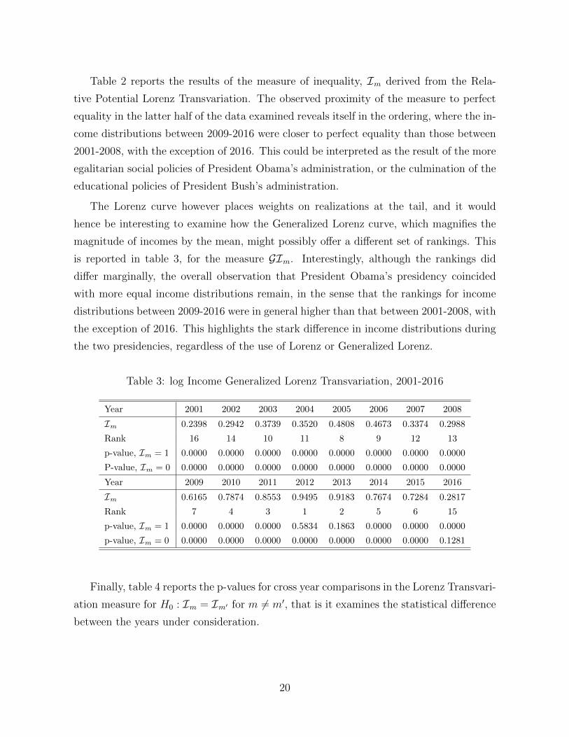
Table 2 reports the results of the measure of inequality, Im derived from the Rela-

tive Potential Lorenz Transvariation. The observed proximity of the measure to perfect

equality in the latter half of the data examined reveals itself in the ordering, where the in-

come distributions between 2009-2016 were closer to perfect equality than those between

2001-2008, with the exception of 2016. This could be interpreted as the result of the more

egalitarian social policies of President Obama’s administration, or the culmination of the

educational policies of President Bush’s administration.

The Lorenz curve however places weights on realizations at the tail, and it would

hence be interesting to examine how the Generalized Lorenz curve, which magnifies the

magnitude of incomes by the mean, might possibly offer a different set of rankings. This

is reported in table 3, for the measure GIm. Interestingly, although the rankings did

differ marginally, the overall observation that President Obama’s presidency coincided

with more equal income distributions remain, in the sense that the rankings for income

distributions between 2009-2016 were in general higher than that between 2001-2008, with

the exception of 2016. This highlights the stark difference in income distributions during

the two presidencies, regardless of the use of Lorenz or Generalized Lorenz.

Table 3: log Income Generalized Lorenz Transvariation, 2001-2016

Year 2001 2002 2003 2004 2005 2006 2007 2008

Im 0.2398 0.2942 0.3739 0.3520 0.4808 0.4673 0.3374 0.2988

Rank 16 14 10 11 8 9 12 13

p-value, Im = 1 0.0000 0.0000 0.0000 0.0000 0.0000 0.0000 0.0000 0.0000

P-value, Im = 0 0.0000 0.0000 0.0000 0.0000 0.0000 0.0000 0.0000 0.0000

Year 2009 2010 2011 2012 2013 2014 2015 2016

Im 0.6165 0.7874 0.8553 0.9495 0.9183 0.7674 0.7284 0.2817

Rank 7 4 3 1 2 5 6 15

p-value, Im = 1 0.0000 0.0000 0.0000 0.5834 0.1863 0.0000 0.0000 0.0000

p-value, Im = 0 0.0000 0.0000 0.0000 0.0000 0.0000 0.0000 0.0000 0.1281

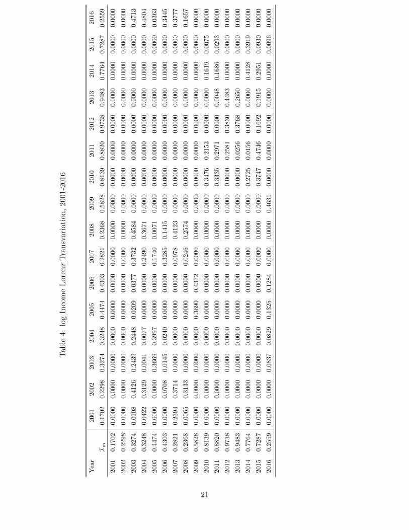
Finally, table 4 reports the p-values for cross year comparisons in the Lorenz Transvari-

ation measure for H0 : Im = Im′ for m 6= m′, that is it examines the statistical difference

between the years under consideration.

20

Tab

le4:

log

Inco

me

Lor

enz

Tra

nsv

aria

tion

,20

01-2

016

Yea

r20

0120

0220

032004

2005

2006

2007

2008

2009

2010

2011

2012

2013

2014

2015

2016

I m0.

1702

0.22

980.

3274

0.3

248

0.4

474

0.4

303

0.2

821

0.2

368

0.5

828

0.8

139

0.8

820

0.9

738

0.9

483

0.7

764

0.7

287

0.2

559

2001

0.17

020.

0000

0.00

000.

0000

0.0

000

0.0

000

0.0

000

0.0

000

0.0

000

0.0

000

0.0

000

0.0

000

0.0

000

0.0

000

0.0

000

0.0

000

0.0

000

2002

0.22

980.

0000

0.00

000.

0000

0.0

000

0.0

000

0.0

000

0.0

000

0.0

000

0.0

000

0.0

000

0.0

000

0.0

000

0.0

000

0.0

000

0.0

000

0.0

000

2003

0.32

740.

0108

0.41

260.

2439

0.2

448

0.0

209

0.0

377

0.3

732

0.4

584

0.0

000

0.0

000

0.0

000

0.0

000

0.0

000

0.0

000

0.0

000

0.4

713

2004

0.32

480.

0422

0.31

290.

0041

0.0

077

0.0

000

0.0

000

0.2

490

0.3

671

0.0

000

0.0

000

0.0

000

0.0

000

0.0

000

0.0

000

0.0

000

0.4

804

2005

0.44

740.

0000

0.00

000.

3669

0.3

997

0.0

000

0.0

000

0.1

740

0.0

071

0.0

000

0.0

000

0.0

000

0.0

000

0.0

000

0.0

000

0.0

000

0.0

363

2006

0.43

030.

0000

0.07

080.

0145

0.0

240

0.0

000

0.0

000

0.3

285

0.1

415

0.0

000

0.0

000

0.0

000

0.0

000

0.0

000

0.0

000

0.0

000

0.3

445

2007

0.28

210.

2394

0.37

140.

0000

0.0

000

0.0

000

0.0

000

0.0

978

0.4

123

0.0

000

0.0

000

0.0

000

0.0

000

0.0

000

0.0

000

0.0

000

0.3

777

2008

0.23

680.

0065

0.31

330.

0000

0.0

000

0.0

000

0.0

000

0.0

246

0.2

574

0.0

000

0.0

000

0.0

000

0.0

000

0.0

000

0.0

000

0.0

000

0.1

657

2009

0.58

280.

0000

0.00

000.

0000

0.0

000

0.3

690

0.4

372

0.0

000

0.0

000

0.0

000

0.0

000

0.0

000

0.0

000

0.0

000

0.0

000

0.0

000

0.0

000

2010

0.81

390.

0000

0.00

000.

0000

0.0

000

0.0

000

0.0

000

0.0

000

0.0

000

0.0

000

0.3

476

0.2

153

0.0

000

0.0

000

0.1

619

0.0

075

0.0

000

2011

0.88

200.

0000

0.00

000.

0000

0.0

000

0.0

000

0.0

000

0.0

000

0.0

000

0.0

000

0.3

335

0.2

971

0.0

000

0.0

048

0.1

686

0.0

293

0.0

000

2012

0.97

380.

0000

0.00

000.

0000

0.0

000

0.0

000

0.0

000

0.0

000

0.0

000

0.0

000

0.0

000

0.2

581

0.3

830

0.4

483

0.0

000

0.0

000

0.0

000

2013

0.94

830.

0000

0.00

000.

0000

0.0

000

0.0

000

0.0

000

0.0

000

0.0

000

0.0

000

0.0

000

0.0

256

0.3

768

0.2

650

0.0

000

0.0

000

0.0

000

2014

0.77

640.

0000

0.00

000.

0000

0.0

000

0.0

000

0.0

000

0.0

000

0.0

000

0.0

000

0.2

725

0.0

156

0.0

000

0.0

000

0.4

128

0.3

919

0.0

000

2015

0.72

870.

0000

0.00

000.

0000

0.0

000

0.0

000

0.0

000

0.0

000

0.0

000

0.0

000

0.3

747

0.4

746

0.1

692

0.1

915

0.2

951

0.0

930

0.0

000

2016

0.25

590.

0000

0.00

000.

0837

0.0

829

0.1

325

0.1

284

0.0

000

0.0

000

0.4

631

0.0

000

0.0

000

0.0

000

0.0

000

0.0

000

0.0

096

0.0

000

21

5 Conclusion

This paper provides the exact limit distributions of transvariation measures applied to the

(Generalized) Lorenz curves. The idea behind transvariation is to ameliorate the common

problem of a lack of resolution in the ranking of Lorenz curves, particularly when they

cross which occurs with regular frequency in empirical work. These crossings in turn

complicate comparisons of Lorenz curves since it would necessitate the estimation of their

location. The convergence of the proposed transvariation measures in turn justifies the

use of subsampling techniques in performing these inferences in lieu of the crossing, thus

reducing the complexity, which was demonstrated in the example.

References

Anderson, G. and Leo, T. W. (2017a). On Providing a Complete Ordering of Non-

Combinable Alternative Prospects. University of Toronto Discussion Paper.

Anderson, G. and Leo, T. W. (2017b). On Solving (Generalized) Gini and Lorenz Com-

parison Issues with Gini’s (Adapted) Transvariation. University of Toronto Discussion

Paper.

Anderson, G., Post, T., and Whang, Y.-J. (2017). Somewhere Between Utopia and

Dystopia: Choosing From Multiple Incomparable Prospect. University of Toronto Dis-

cussion Paper.

Atkinson, A. B. (1970). On the Measurement of Inequality. Journal of Economic Theory,

2(3), 244–263.

Beach, C. M. and Davidson, R. (1983). Distribution-Free Statistical Inference with Lorenz

Curves and Income Shares. The Review of Economic Studies, 50(4), 723–735.

Gini, C. (1916). Il Concetto di Transvariazione e le sue Prime Applicazioni. In C. Gini

(Ed.), Transvariazione. Libreria Goliardica, (1–55).

Gini, C. (1959). Transvariazione. Libreria Goliardica, Rome.

Leshno, M. and Levy, H. (2002). Preferred by “All” and Preferred by “Most” Decision

Makers: Almost Stochastic Dominance. Management Science, 48(8), 1074–1085.

22

Linton, O., Maasoumi, E., and Whang, Y.-J. (2005). Consistent Testing for Stochastic

Dominance under General Sampling Schemes. The Review of Economic Studies, 72,

735–765.

Linton, O., Post, T., and Whang, Y.-J. (2014). Testing for the Stochastic Dominance

Efficiency of a Given Portfolio. The Econometrics Journal, 17, S59–S74.

Politis, D. N. and Romano, J. P. (1994). Large Sample Confidence Regions Based on

Subsamples Under Minimal Assumptions. The Annals of Statistics, 22(4), 2031–2050.

Politis, D. N., Romano, J. P., and Wolf, M. (1999). Subsampling. New York: Springer.

Seth, S. and Yalonetzky, G. (2016). Has the World Converged? A Robust Analysis of

Non-Monetary Bounded Indictors. Leeds University Business School Discussion Paper.

Shorrocks, A. F. (1983). Ranking Income Distribution. Economica, 50(197), 3–17.

Zheng, B. (2016). Almost Lorenz Dominance. University of Colorado, Denver, Discussion

Paper.

23