化學鍵

【本著作除另有註明，所有內容皆採用 創用CC 姓名標示-非商業使用-相 同方式分享 3.0 台灣 授權條款釋出】

台灣大學開放式課程

Pictorial → Symmetry → MO AXn n=3, 4, 5, 6

Chemical Bonding

Lecture 10: MO for AXn system, Multicenter Bonding, VSEPR,

Hybridization

Spring 2012

5/11/2012

Molecular Orbitals for σ Bonding in AXn Molecules

A X1

X2

X 3

X4

y

z

r1

r2 r3 x

r4

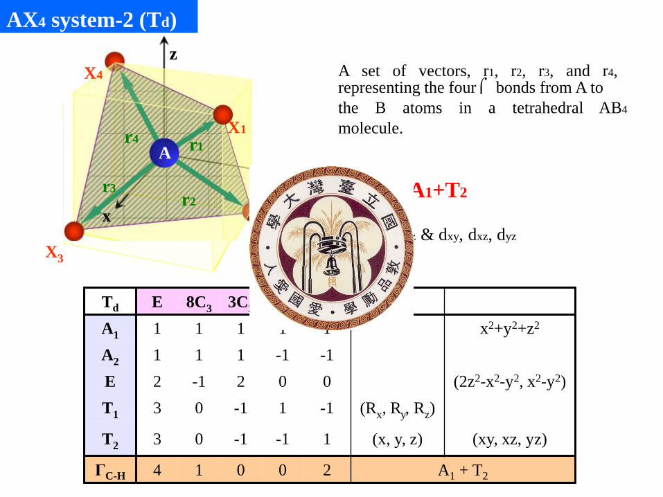
A set of vectors, r1, r2, r3, and r4, representing the four ⌠ bonds from A to the B atoms in a tetrahedral AB4

molecule.

ΓA-B = A1+T2 A1: s T2: px,py,pz & dxy, dxz, dyz

AX4 system-2 (Td)

Td E 8C3 3C2 6S4 6σd A1 1 1 1 1 1 x2+y2+z2 A2 1 1 1 -1 -1 E 2 -1 2 0 0 (2z2-x2-y2, x2-y2) T1 3 0 -1 1 -1 (Rx, Ry, Rz)

T2 3 0 -1 -1 1 (x, y, z) (xy, xz, yz)

ΓC-H 4 1 0 0 2 A1 + T2

Ene

rgy

Ψb

s + (σ1+ σ2+ σ3+ σ4)

Ψa

s − (σ1+ σ2+ σ3+ σ4)

A atom X atoms MOs

AX4 system-2 (Td)

a1

a1

s a1 σ1+ σ2+ σ3+ σ4 a1

By combining the central s orbital with ligand orbital SALC (symmetry-adapted linear combinations) to give either positive or negative overlap, we get Ψb and Ψa, respectively. The expressions written for these are only meant to express this sign relationship; the actual expression for Ψa and Ψ b contain different coefficients.

Ene

rgy

A atom X atoms MOs

?

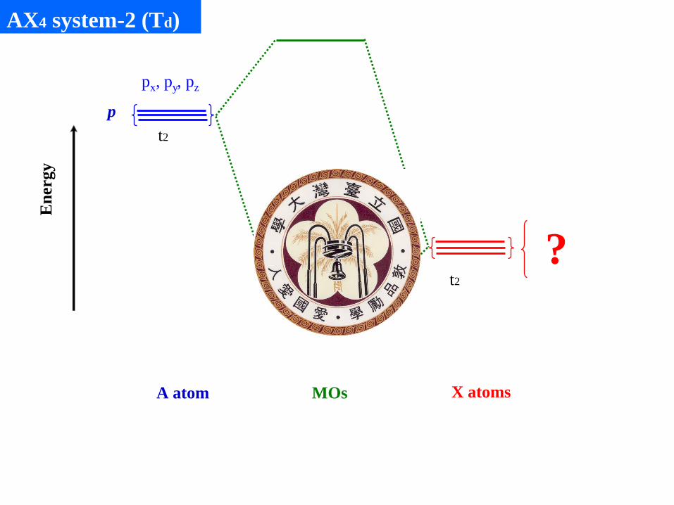
AX4 system-2 (Td)

p t2

t2

px, py, pz

+

+

+

−

−

− +

+

+

−

−

−

+ +

+

−

− −

AX4 system-2 (Td)

Consider ligand group orbitals (LGOs) that match with each of the center-atom atomic orbitals Symmetry-adapted linear combination (SALC) Note that s or p along the axis both can form the σ bond

Qualitative representations of the three T2 type σ MOs for an AX4 molicule.

Ene

rgy

Ψ a(T2)

Ψ b(T2) Ψ b(A1)

A atom B atoms MOs

etc.

AX4 system-2 (Td)

Ψ a(A1) p t2 s a1

σ1+ σ2+ σ3+ σ4

σ1− σ2+ σ3− σ4

a1+ t2

An MO energy level diagram for a AX4 molecule showing both the A1 and T2 type interaction.

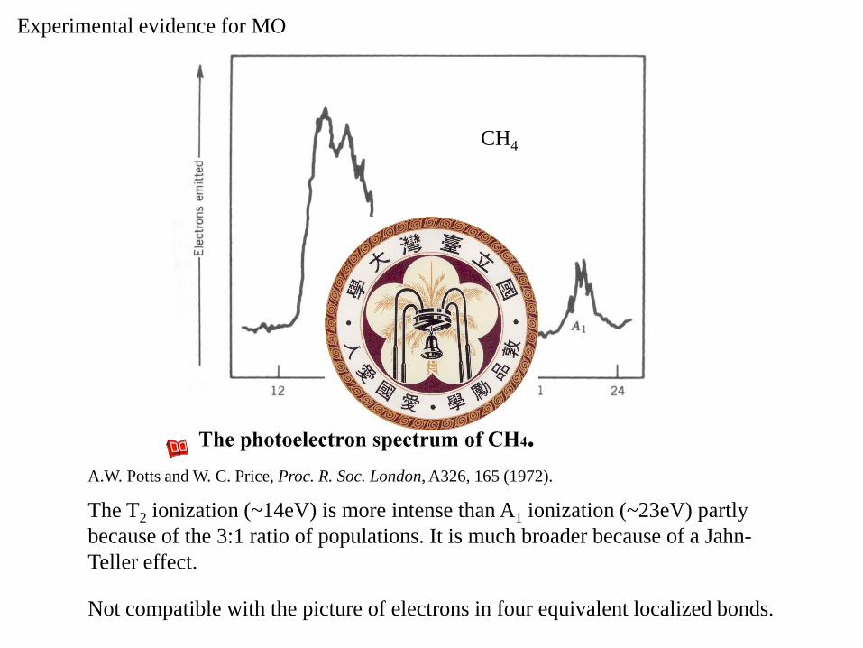
Experimental evidence for MO

Not compatible with the picture of electrons in four equivalent localized bonds.

A.W. Potts and W. C. Price, Proc. R. Soc. London, A326, 165 (1972).

The T2 ionization (~14eV) is more intense than A1 ionization (~23eV) partly because of the 3:1 ratio of populations. It is much broader because of a Jahn-Teller effect.

CH4

AX4 system-1 (D4h) XeF4

F

F

F x

y F Xe

Γπ’ : out of plane Γπ” : in plane

s+dx2-y2+(px+py) Xe: dsp2

D4h E 2C4 (z) C2 2C'2 2C''2 i 2S4 σh 2σv 2σd A1g 1 1 1 1 1 1 1 1 1 1 x2+y2, z2 A2g 1 1 1 -1 -1 1 1 1 -1 -1 Rz B1g 1 -1 1 1 -1 1 -1 1 1 -1 x2-y2 B2g 1 -1 1 -1 1 1 -1 1 -1 1 xy Eg 2 0 -2 0 0 2 0 -2 0 0 (Rx, Ry) (xz, yz) A1u 1 1 1 1 1 -1 -1 -1 -1 -1 A2u 1 1 1 -1 -1 -1 -1 -1 1 1 z B1u 1 -1 1 1 -1 -1 1 -1 -1 1 B2u 1 -1 1 -1 1 -1 1 -1 1 -1 Eu 2 0 -2 0 0 -2 0 2 0 0 (x, y) Γσ 4 0 0 2 0 0 0 4 2 0 A1g + B1g + Eu

Γπ’ 4 0 0 -2 0 0 0 -4 2 0 A2u + B2u + Eg

Γπ” 4 0 0 -2 0 0 0 4 -2 0 A2g+ B2g + Eu

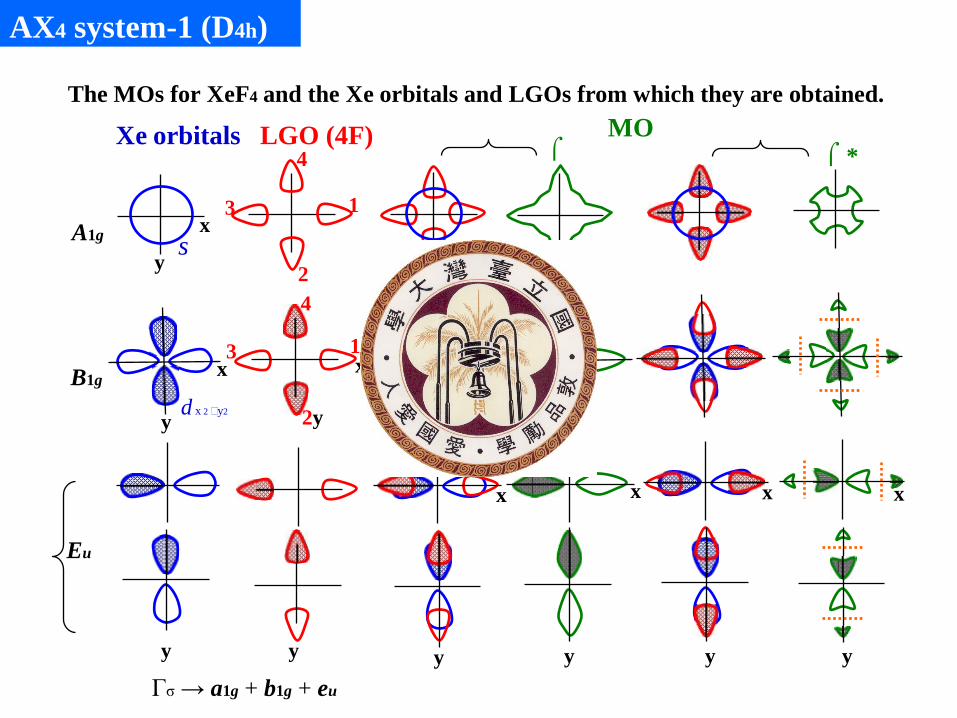
The MOs for XeF4 and the Xe orbitals and LGOs from which they are obtained.

AX4 system-1 (D4h)

MO

A1g

B1g

Eu

⌠* ⌠

4

1 x

1

2

3

Xe orbitals LGO (4F) 4

2y

y

x s

y

3 x d x 2 �y2

y y

Γσ → a1g + b1g + eu

x x

y y

x

y

x

y

AX4 system-1 (D4h)

LGO – Symmetry adapted Group orbitals

dsp2

Xe XeF4 4F

2p (12)

5p

a1g* eu*

2s (4) b1g

eu a1g

a2u(pz)

5s a1g

eu a2u

(a1g + b1g + b2g + eg) 5d eg(dxz,dyz) a1g(dz2)

b1g* b2g(dxy)

a2u eu a1g

a2g+b2g+eu+a2u+b2u+eg nonbonding a1g+b1g+eu nonbonding

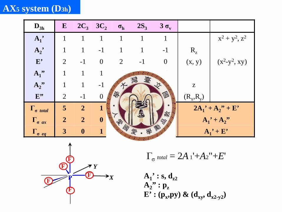
AX5 system (D3h)

A1’ : s, dz2 A2” : pz E’ : (px,py) & (dxy, dx2-y2)

Γ total = 2A 1'+A2"+E' σ

X

Y F P

F

F F

F

D3h E 2C3 3C2 σh 2S3 3 σv

A1’ 1 1 1 1 1 1 x2 + y2, z2

A2’ 1 1 -1 1 1 -1 Rz

E’ 2 -1 0 2 -1 0 (x, y) (x2-y2, xy) A1” 1 1 1 -1 -1 -1

A2” 1 1 -1 -1 -1 1 z

E” 2 -1 0 -2 1 0 (Rx,Ry)

Γσ total 5 2 1 3 0 3 2A1’ + A2” + E’ Γσ ax 2 2 0 0 0 2 A1’ + A2” Γσ eq 3 0 1 3 0 1 A1’ + E’

Molecular orbitals for σ bonding in PF5

Γσ → 2A1’ + E’ + A2”

a1’

a1’

a2”

e’

e’

⌠ MO (AX5)

2 z

P orbitals (A) s + d

2 z s � d

px

pz

py

LGO (5X) 4 5

2

3

1

2

3

1

4

5

1

3

2

3

1

4

5

2

3

1

1

3

AX5 system (D3h)

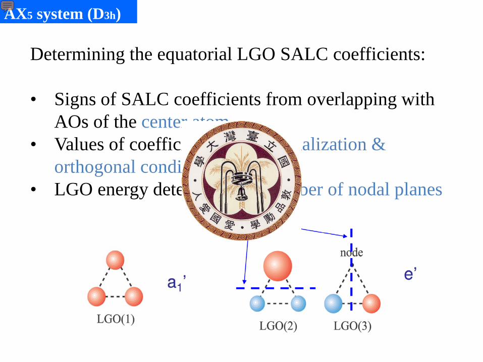
AX5 system (D3h)

Determining the equatorial LGO SALC coefficients: • Signs of SALC coefficients from overlapping with

AOs of the center atom • Values of coefficients from normalization &

orthogonal conditions • LGO energy determined by number of nodal planes

AX5 system (D3h)

a1’

a1’

a2”

e’

σ MO (AX5)

2

3

1

4

5

2

3

1 1

e’ 3

A2 (axial) = ± pz 1 2

'' (σ 4 −σ5)

A 1 (axial) = 1 2

' ±dz2 (σ 4 +σ5)

E (equatorial) = ' 1 6 1 2

=

(2σ2 −σ 1 −σ3)

(σ 1 −σ3)

px py

±

SALC of X A

(σ1 +σ 2 +σ3) A 1 (equatorial) = 1 3

' ± s

a2

P PF5 5F

P (15 orbitals) s (5)

1e’ 1a2” 1a1’

2a1 ’

px, py pz s

e’ ” a1’

e’ e” a1’

d dz2

4a1 2a2” 2e’ 3a1’

e’

e”

AX5 system (D3h)

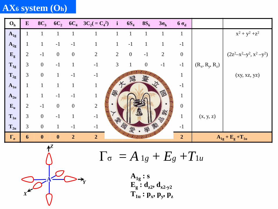
AX6 system (Oh)

A1g : s Eg : dz2, dx2-y2 T1u : px, py, pz

A

Z

Y

X

Γσ = A 1g + Eg +T1u

Oh E 8C3 6C2 6C4 3C2( = C42) i 6S4 8S6 3σh 6 σd

A1g 1 1 1 1 1 1 1 1 1 1 x2 + y2 +z2

A2g 1 1 -1 -1 1 1 -1 1 1 -1

Eg 2 -1 0 0 2 2 0 -1 2 0 (2z2–x2–y2, x2 –y2)

T1g 3 0 -1 1 -1 3 1 0 -1 -1 (Rx, Ry, Rz)

T2g 3 0 1 -1 -1 3 -1 0 -1 1 (xy, xz, yz)

A1u 1 1 1 1 1 -1 -1 -1 -1 -1

A2u 1 1 -1 -1 1 -1 1 -1 -1 1

Eu 2 -1 0 0 2 -2 0 1 -2 0

T1u 3 0 -1 1 -1 -3 -1 0 1 1 (x, y, z)

T2u 3 0 1 -1 -1 -3 1 0 1 -1

Γσ 6 0 0 2 2 0 0 0 4 2 A1g + Eg +T1u

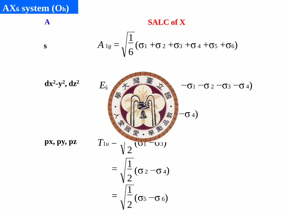
AX6 system (Oh)

1 6

(σ1 +σ 2 +σ3 +σ 4 +σ5 +σ6) A 1g =

1 12

(2σ5 +2σ6 −σ1 −σ 2 −σ3 −σ 4) Eg =

1 2

= (σ1 −σ 2 +σ3 −σ 4)

1 2 1 2 1 2

T1u =

=

=

(σ1 −σ3)

(σ 2 −σ 4)

(σ5 −σ 6)

s

dx2-y2, dz2

px, py, pz

SALC of X A

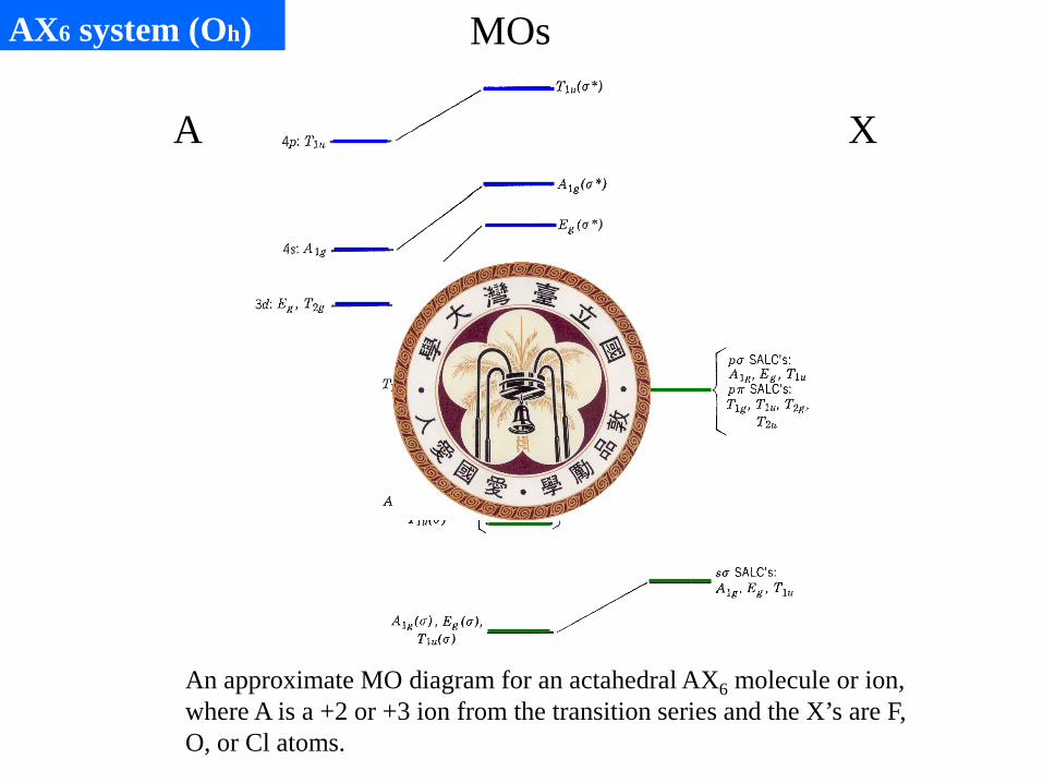
A orbitals 6X orbitals MOs

σ SALCs of A1g Eg, T1u Symmetry

dz2 dx2�y2

px、py、pz

a1g*

t1u*

eg* s

t1u eg a1g

AX6 system (Oh)

Molecular Orbitals for π Bonding in AXn Molecules

Character table for D3h point group

D3h E 2C3 3C'2 σh 2S3 3σv

A'1 1 1 1 1 1 1 x2+y2, z2 A'2 1 1 -1 1 1 -1 Rz E' 2 -1 0 2 -1 0 (x, y) (x2-y2, xy)

A''1 1 1 1 -1 -1 -1 A''2 1 1 -1 -1 -1 1 z E'' 2 -1 0 -2 1 0 (Rx, Ry) (xz, yz)

ΓS-O(σ) 3 0 1 3 0 1 A1’ + E’

1

2

1

1' [1 3 1 2 0 1 3 1 1 1 3 1 2 0 1 3 1 1] 1121' [1 3 1 2 0 1 3 1 ( 1) 1 3 1 2 0 1 3 1 ( 1)] 0

121' [1 3 2 2 0 ( 1) 3 1 0 1 3 2 2 0 ( 1) 3 1 0 ]1

121'' [1 3 1 2 0 1 3 1 1 1 3 ( 1) 2 0 ( 1) 3 1

12

nA

nA

E

nA

= × × + × × + × × + × × + × × + × × =

= × × + × × + × × − + × × + × × + × × − =

= × × + × × − + × × + × × + × × − + × × =

= × × + × × + × × + × × − + × × − + ×

2

( 1)] 0

1'' [1 3 1 2 0 1 3 1 ( 1) 1 3 ( 1) 2 0 ( 1) 3 1 1] 012

1'' [1 3 2 2 0 ( 1) 3 1 0 1 3 ( 2 ) 2 0 1 3 1 0 ] 012

nA

E

× − =

= × × + × × + × × − + × × − + × × − + × × =

= × × + × × − + × × + × × − + × × + × × =

A’1 + E’ ΓS-O(σ)

σ bonding

Character table for D3h point group

D3h E 2C3 3C'2 σh 2S3 3σv

A'1 1 1 1 1 1 1 x2+y2, z2

A'2 1 1 -1 1 1 -1 Rz

E' 2 -1 0 2 -1 0 (x, y) (x2-y2, xy)

A''1 1 1 1 -1 -1 -1

A''2 1 1 -1 -1 -1 1 z

E'' 2 -1 0 -2 1 0 (Rx, Ry) (xz, yz)

ΓS-O(π⊥) 3 0 -1 -3 0 1 A2” +E”

1

2

1

1' [1 3 1 2 0 1 3 ( 1) 1 1 ( 3) 1 2 0 1 3 1 1] 0121' [1 3 1 2 0 1 3 ( 1) ( 1) 1 ( 3) 1 2 0 1 3 1 ( 1)] 0

121' [1 3 2 2 0 ( 1) 3 ( 1) 0 1 ( 3) 2 2 0 ( 1) 3 1 0 ] 0

121'' [1 3 1 2 0 1 3 ( 1) 1

12

nA

nA

E

nA

= × × + × × + × − × + × − × + × × + × × =

= × × + × × + × − × − + × − × + × × + × × − =

= × × + × × − + × − × + × − × + × × − + × × =

= × × + × × + × − × +

2

1 ( 3) ( 1) 2 0 ( 1) 3 1 ( 1)] 0

1'' [1 3 1 2 0 1 3 ( 1) ( 1) 1 ( 3) ( 1) 2 0 ( 1) 3 1 1] 112

1'' [1 3 2 2 0 ( 1) 3 ( 1) 0 1 ( 3) ( 2 ) 2 0 1 3 1 0 ] 112

nA

E

× − × − + × × − + × × − =

= × × + × × + × − × − + × − × − + × × − + × × =

= × × + × × − + × − × + × − × − + × × + × × =

A’’2 + E’’

ΓS-O(π⊥)

π⊥ bonding

Character table for D3h point group D3h E 2C3 3C'2 σh 2S3 3σv A'1 1 1 1 1 1 1 x2+y2, z2 A'2 1 1 -1 1 1 -1 Rz E' 2 -1 0 2 -1 0 (x, y) (x2-y2, xy)

A''1 1 1 1 -1 -1 -1 A''2 1 1 -1 -1 -1 1 z E'' 2 -1 0 -2 1 0 (Rx, Ry) (xz, yz)

ΓS-O(π//) 3 0 -1 3 0 -1 A’2 + E’

1

2

1

1' [1 3 1 2 0 1 3 ( 1) 1 1 3 1 2 0 1 3 ( 1) 1] 0121' [1 3 1 2 0 1 3 ( 1) ( 1) 1 3 1 2 0 1 3 ( 1) ( 1)] 1

121' [1 3 2 2 0 ( 1) 3 ( 1) 0 1 3 2 2 0 ( 1) 3 ( 1) 0] 1

121'' [1 3 1 2 0 1 3 ( 1) 1

12

nA

nA

E

nA

= × × + × × + × − × + × × + × × + × − × =

= × × + × × + × − × − + × × + × × + × − × − =

= × × + × × − + × − × + × × + × × − + × − × =

= × × + × × + × − × +

2

1 3 ( 1) 2 0 ( 1) 3 ( 1) ( 1)] 0

1'' [1 3 1 2 0 1 3 ( 1) ( 1) 1 3 ( 1) 2 0 ( 1) 3 ( 1) 1] 012

1'' [1 3 2 2 0 ( 1) 3 ( 1) 0 1 3 ( 2 ) 2 0 1 3 ( 1) 0 ] 012

nA

E

× × − + × × − + × − × − =

= × × + × × + × − × − + × × − + × × − + × − × =

= × × + × × − + × − × + × × − + × × + × − × =

A’2 + E’

ΓS-O(π//)

π// bonding

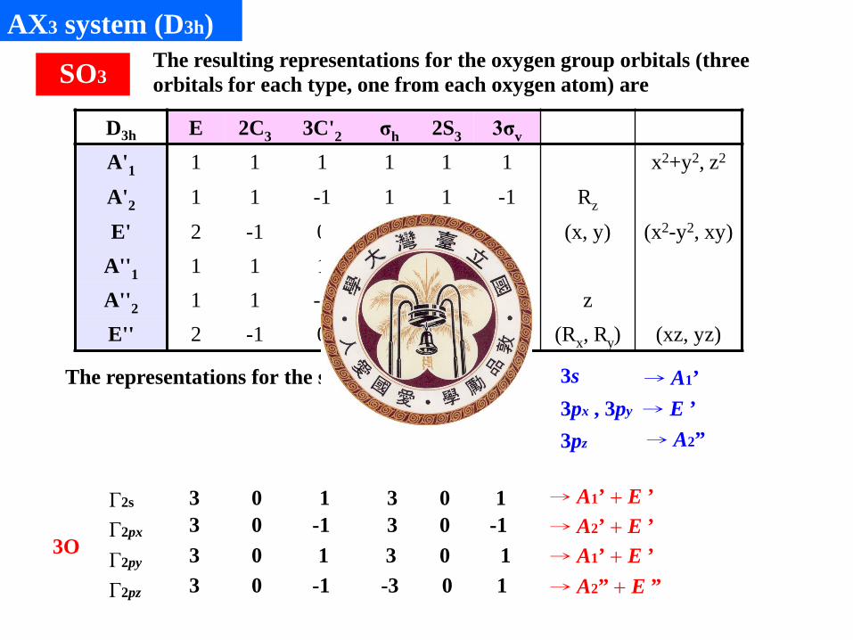
SO3 The resulting representations for the oxygen group orbitals (three orbitals for each type, one from each oxygen atom) are

The representations for the sulfur orbitals

3O

→ A1’ + E ’ → A2’ + E ’ → A1’ + E ’ → A2” + E ”

Γ2s

Γ2px

Γ2py

Γ2pz

3 3 3 3

0 0 0 0

1 -1 1 -1

3 3 3 -3

0 0 0 0

1 -1 1 1

S

AX3 system (D3h)

D3h E 2C3 3C'2 σh 2S3 3σv A'1 1 1 1 1 1 1 x2+y2, z2 A'2 1 1 -1 1 1 -1 Rz E' 2 -1 0 2 -1 0 (x, y) (x2-y2, xy)

A''1 1 1 1 -1 -1 -1 A''2 1 1 -1 -1 -1 1 z E'' 2 -1 0 -2 1 0 (Rx, Ry) (xz, yz)

3s → A1’ 3px , 3py → E ’ 3pz → A2”

The molecular orbitals resulting from combining these orbitals are shown as figure. z

x

x x

x

y y y

y

z z

z

pz

A2” + E ”

Oxygen orbitals px py

A2’ + E ’ A1’ + E ’ s A1’

pz

A2”

Sulfur orbitals px ; py E ’

AX3 system (D3h)

LGO or SALC s A1’ + E ’

sσ π// pσ π⊥

y direction is along each S=O bond

AX3 system (D3h)

2e’

3e’ 4a1’

1e”

Qualitative MO energy-level diagram for SO3 5e’ 5a1’ 2a2”

1a2’ 1a2” 4e’

3a1’ 2s

2p

3s

3p

S 3O SO3

A1’

A2’’ + E’

A1’+ E’

A1’ + E’ A2’ + E’ A2” + E”

pσ π//

π⊥

sσ

A set of vectors representing the four π-type p orbitals on the four B atoms in a tetrahedral AB4 molecule.

Γπ = E+T1+T2 E: dz2, dx2-y2 T1: None T2: px,py,pz & dxy, dxz, dyz

AX4 system-2 (Td)

Td E 8C3 3C2 6S4 6σd A1 1 1 1 1 1 x2+y2+z2 A2 1 1 1 -1 -1 E 2 -1 2 0 0 (2z2-x2-y2, x2-y2) T1 3 0 -1 1 -1 (Rx, Ry, Rz)

T2 3 0 -1 -1 1 (x, y, z) (xy, xz, yz)

Γπ 8 -1 0 0 0 E + T1 + T2

A set of vectors representing the four π-type p orbitals on the four B atoms in a tetrahedral AB4 molecule.

Γπ = E+T1+T2

E: dz2, dx2-y2 T1: None T2: px,py,pz & dxy, dxz, dyz

AX4 system-2 (Td)

• It is impossible to form a complete set of π bonds (i.e. two to each X atom)

• The π bonding will not be entirely independent of the σ bonding

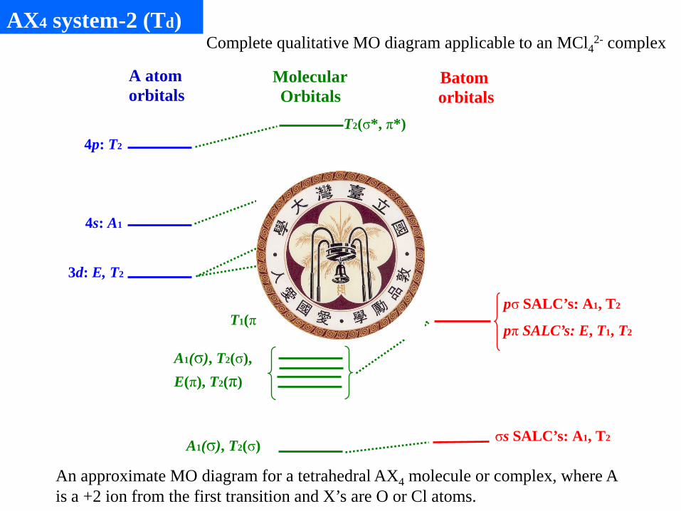
A atom orbitals

Batom orbitals

Molecular Orbitals

pσ SALC’s: A1, T2

pπ SALC’s: E, T1, T2 σs SALC’s: A1, T2

T2(σ*, π*) E(π*)

T1(π) A1(σ), T2(σ), E(π), T2(π) A1(σ), T2(σ)

T2(σ*, π*) 4p: T2 A1(σ*)

4s: A1 3d: E, T2

AX4 system-2 (Td) Complete qualitative MO diagram applicable to an MCl4

2- complex

An approximate MO diagram for a tetrahedral AX4 molecule or complex, where A is a +2 ion from the first transition and X’s are O or Cl atoms.

AX6 system (Oh)

T1g : None T2g : dxz, dyz, dxy

T1u : px, py, pz

T2u : None

Γπ = T1g+T2g+T1u+T2u

Oh E 8C3 6C2 6C4 3C2( = C42) i 6S4 8S6 3σh 6 σd

A1g 1 1 1 1 1 1 1 1 1 1 x2 + y2 +z2

A2g 1 1 -1 -1 1 1 -1 1 1 -1

Eg 2 -1 0 0 2 2 0 -1 2 0 (2z2–x2–y2, x2 –y2)

T1g 3 0 -1 1 -1 3 1 0 -1 -1 (Rx, Ry, Rz)

T2g 3 0 1 -1 -1 3 -1 0 -1 1 (xy, xz, yz)

A1u 1 1 1 1 1 -1 -1 -1 -1 -1

A2u 1 1 -1 -1 1 -1 1 -1 -1 1

Eu 2 -1 0 0 2 -2 0 1 -2 0

T1u 3 0 -1 1 -1 -3 -1 0 1 1 (x, y, z)

T2u 3 0 1 -1 -1 -3 1 0 1 -1

Γπ 12 0 0 0 -4 0 0 0 0 0 T1g + T2g +T1u + T2u

AX6 system (Oh)

px1

px4

py2

py3

px3

px5

py6

py1

py5

px2

px6

py4

T2g SALC of X atom πorbitals are derived by matching to T2g orbitals (dxy, dxz, dyz) on the A atom.

AX6 system (Oh)

An approximate MO diagram for an actahedral AX6 molecule or ion, where A is a +2 or +3 ion from the transition series and the X’s are F, O, or Cl atoms.

A X

MOs

Molecular Orbitals for Cyclic Molecules and Multicenter

Bonding

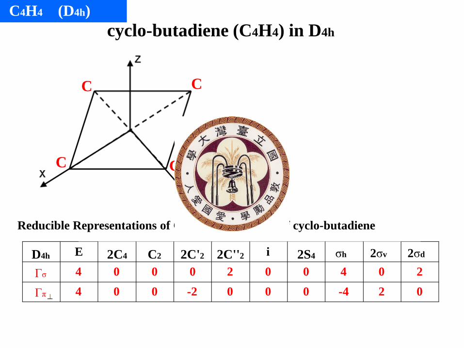
cyclo-butadiene (C4H4) in D4h

D4h E 2C4 C2 2C'2 2C''2 i 2S4 σh 2σv 2σd

Γσ

Γπ

4 4

0 0

0 0

0 -2

2 0

0 0

0 0

4 -4

0 2

2 0

C

C C

C

Reducible Representations of C-C σ- and π-bonds of cyclo-butadiene

C4H4 (D4h)

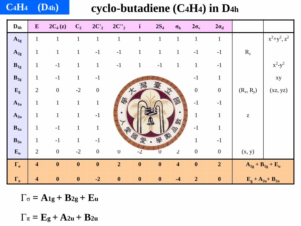
Γσ = A1g + B2g + Eu

Γπ = Eg + A2u + B2u

cyclo-butadiene (C4H4) in D4h C4H4 (D4h)

D4h E 2C4 (z) C2 2C'2 2C''2 i 2S4 σh 2σv 2σd

A1g 1 1 1 1 1 1 1 1 1 1 x2+y2, z2

A2g 1 1 1 -1 -1 1 1 1 -1 -1 Rz

B1g 1 -1 1 1 -1 1 -1 1 1 -1 x2-y2

B2g 1 -1 1 -1 1 1 -1 1 -1 1 xy

Eg 2 0 -2 0 0 2 0 -2 0 0 (Rx, Ry) (xz, yz)

A1u 1 1 1 1 1 -1 -1 -1 -1 -1

A2u 1 1 1 -1 -1 -1 -1 -1 1 1 z

B1u 1 -1 1 1 -1 -1 1 -1 -1 1

B2u 1 -1 1 -1 1 -1 1 -1 1 -1

Eu 2 0 -2 0 0 -2 0 2 0 0 (x, y)

Γσ 4 0 0 0 2 0 0 4 0 2 A1g + B1g + Eu

Γπ 4 0 0 -2 0 0 0 -4 2 0 Eg + A2u+ B2u

C4H4 (D4h) Trick: determining MOs by matching to central atomic orbital with proper symmetries

Γπ = Eg + A2u + B2u

Eg xz, yz

A2u z B2u z(x2-y2)

http://www.chemistry.ucsc.edu/~soliver/151A/Handouts/

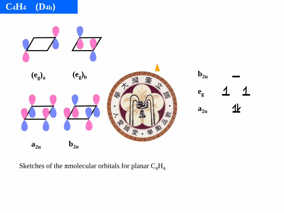
C4H4 (D4h)

Sketches of the πmolecular orbitals for planar C4H4

(eg)a (eg)b

a2u b2u

a2u

b2u

eg

Ener

gy

Diborane (D2h)

Diborane (B2H6) has a planar ethylene-like framework (D2h)

Total 3+3+6 = 12 electrons 2x4 = 8 electrons forming 4 edge B-H bonds 12-8 = 4 electrons in the center square electron deficient

Bridge bond: three atoms sharing 2 electrons Three-center two-electron bond

Diborane (D2h) σ bridge bonding in diborane

Γboron = Ag + B2g + B1u + B3u

ΓH = Ag + B3u

D2h E C2(z) C2(y) C2(x) i σ(xy) σ(xz) σ(yz) Ag 1 1 1 1 1 1 1 1 B1g 1 1 -1 -1 1 1 -1 -1 B2g 1 -1 1 -1 1 -1 1 -1 B3g 1 -1 -1 1 1 -1 -1 1 Au 1 1 1 1 -1 -1 -1 -1 B1u 1 1 -1 -1 -1 -1 1 1 B2u 1 -1 1 -1 -1 1 -1 1 B3u 1 -1 -1 1 -1 1 1 -1

Γboron

4 0 0 0 0 0 4 0

ΓH 2 0 0 2 0 2 2 6

φ1

φ2

φ3

φ4

H1

H2

x

z y

Diborane (D2h) Qualitative energy-level diagram for the bridge bonding in diborane

Four electrons in two bonding orbitals two electron three-center bridge bonds

Γboron = Ag + B2g + B1u + B3u

ΓH= Ag + B3u

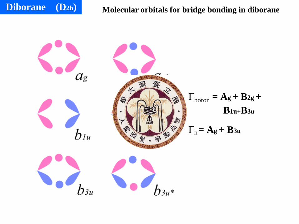
Diborane (D2h) Molecular orbitals for bridge bonding in diborane

Γboron = Ag + B2g + B1u+B3u

ΓH = Ag + B3u

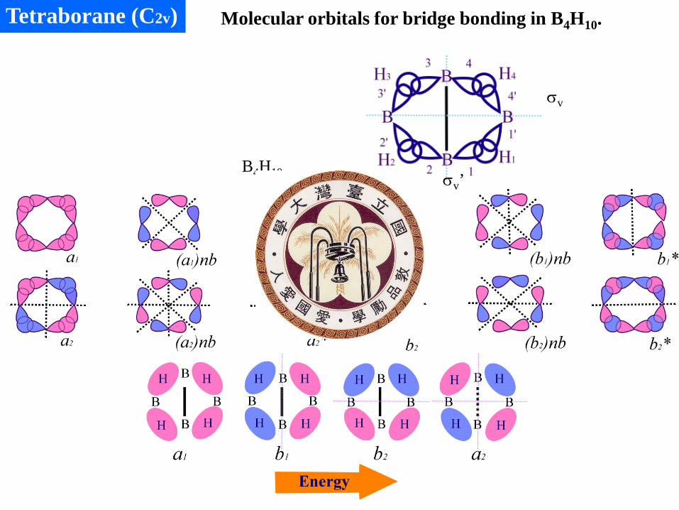
Tetraborane (C2v) Molecular orbitals for bridge bonding in B4H10.

σv

σv’ B4H10

VSEPR & Hybrid Orbitals

Lewis Theory G.N. Lewis, who introduced it in his 1916 article The Molecule and the Atom

Lewis stuctures, also called Electron-dot Structures or Electron-dot Diagrams, are diagrams that show the bonding between atoms of a molecule, and the lone pairs of electrons that may exist in the molecule.

The Octet Rule

Eight electrons in their valence shells, similar to the electronic configuration of a noble gas.

H Cl [Na]+ [ Cl ]−

Lewis Structures：NaCl , HCl and H2O •• H:O:H

•• Sorce from: http://en.wikipedia.org/wiki/Category:Chemical_bonding

Sorce from: http://en.wikipedia.org/wiki/Category:Chemical_bonding

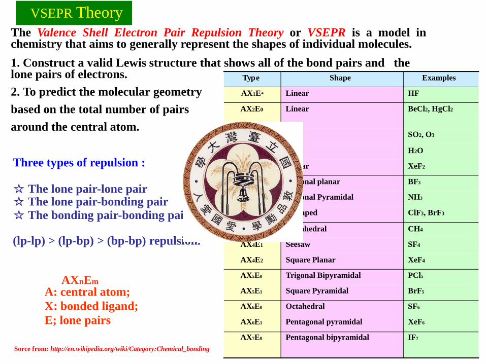
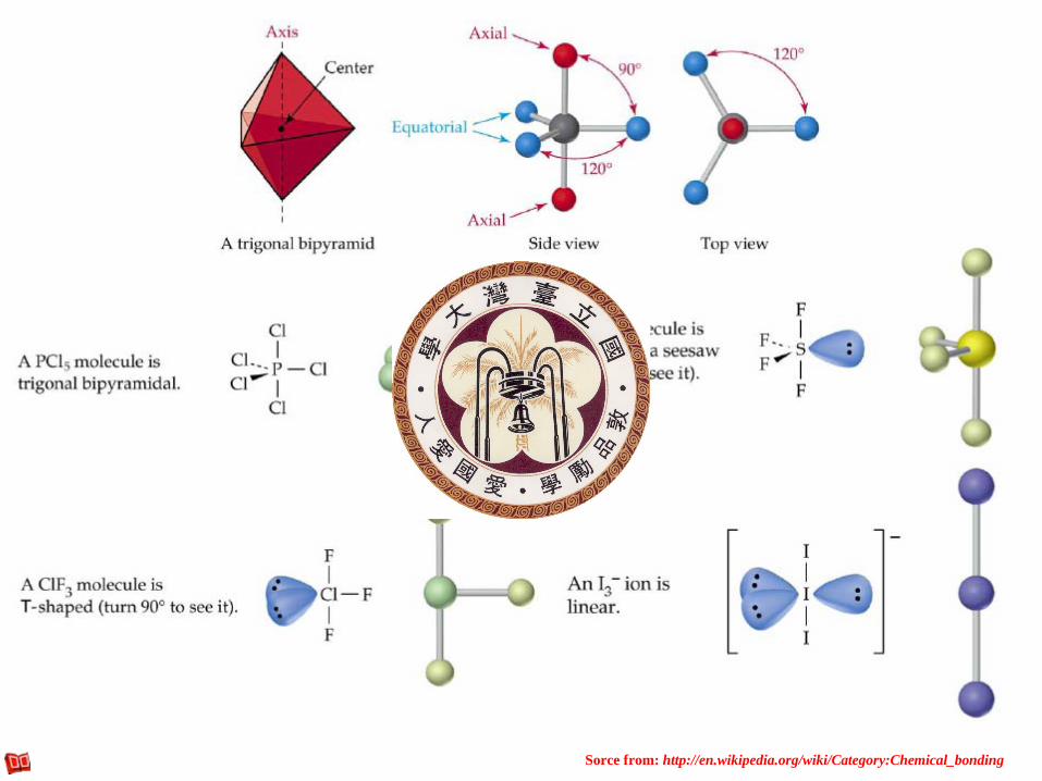
VSEPR Theory The Valence Shell Electron Pair Repulsion Theory or VSEPR is a model in chemistry that aims to generally represent the shapes of individual molecules. 1. Construct a valid Lewis structure that shows all of the bond pairs and the lone pairs of electrons. 2. To predict the molecular geometry based on the total number of pairs around the central atom.

Three types of repulsion :

☆ The lone pair-lone pair ☆ The lone pair-bonding pair ☆ The bonding pair-bonding pair

(lp-lp) > (lp-bp) > (bp-bp) repulsion.

AXnEm A: central atom; X: bonded ligand; E; lone pairs

Type Shape Examples

AX1E* Linear HF

AX2E0 Linear BeCl2, HgCl2

AX2E1 Bent SO2, O3

AX2E2 Bent H2O

AX2E3 Linear XeF2

AX3E0 AX3E1

Trigonal planar Trigonal Pyramidal

BF3 NH3

AX3E2 T-shaped ClF3, BrF3

AX4E0 Tetrahedral CH4

AX4E1 Seesaw SF4

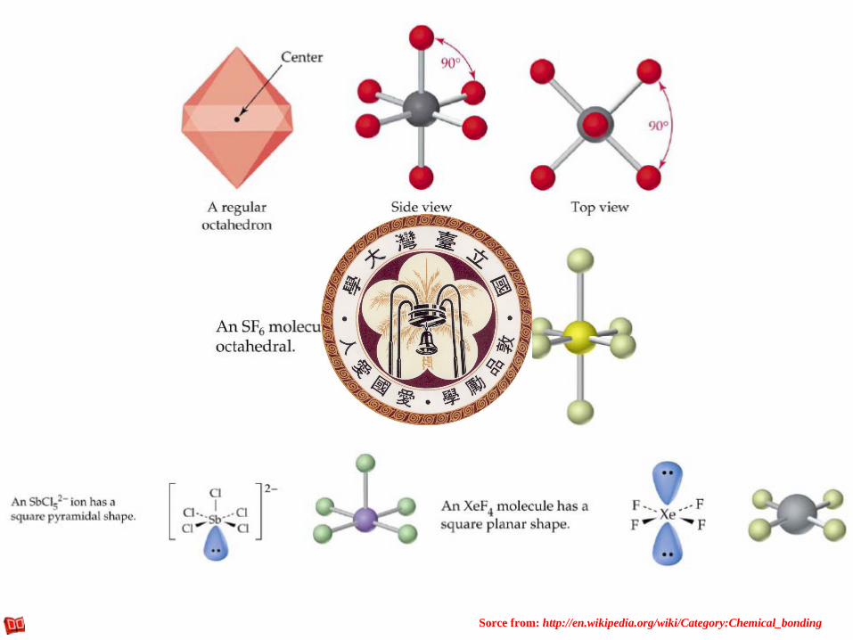
AX4E2 Square Planar XeF4

AX5E0 AX5E1 AX6E0 AX6E1 AX7E0

Trigonal Bipyramidal Square Pyramidal Octahedral Pentagonal pyramidal Pentagonal bipyramidal

PCl5 BrF5 SF6 XeF6 IF7

Sorce from: http://en.wikipedia.org/wiki/Category:Chemical_bonding

Sorce from: http://en.wikipedia.org/wiki/Category:Chemical_bonding

Sorce from: http://en.wikipedia.org/wiki/Category:Chemical_bonding

Sorce from: http://en.wikipedia.org/wiki/Category:Chemical_bonding

Sorce from: http://en.wikipedia.org/wiki/Category:Chemical_bonding

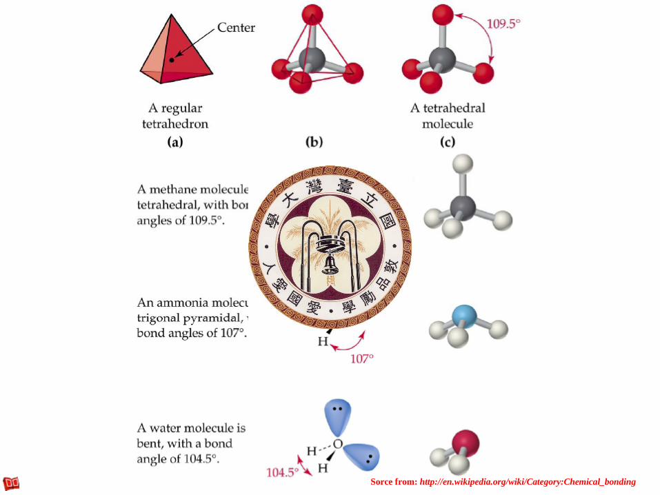
Molecular Geometries around atoms with 2,3,4,5 and 6 charge clouds.

Molecular Geometries around atoms with 2,3,4,5 and 6 charge clouds.

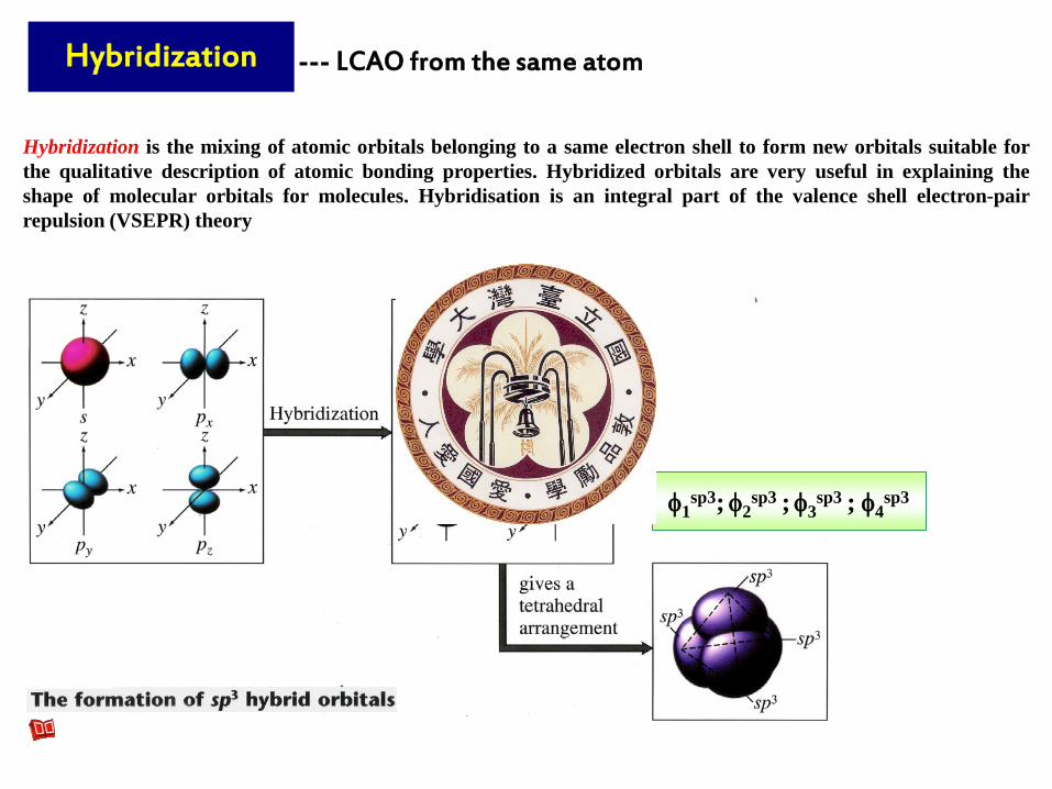
Hybridization

Hybridization is the mixing of atomic orbitals belonging to a same electron shell to form new orbitals suitable for the qualitative description of atomic bonding properties. Hybridized orbitals are very useful in explaining the shape of molecular orbitals for molecules. Hybridisation is an integral part of the valence shell electron-pair repulsion (VSEPR) theory

--- LCAO from the same atom

φ1sp3; φ2

sp3 ; φ3sp3 ; φ4

sp3

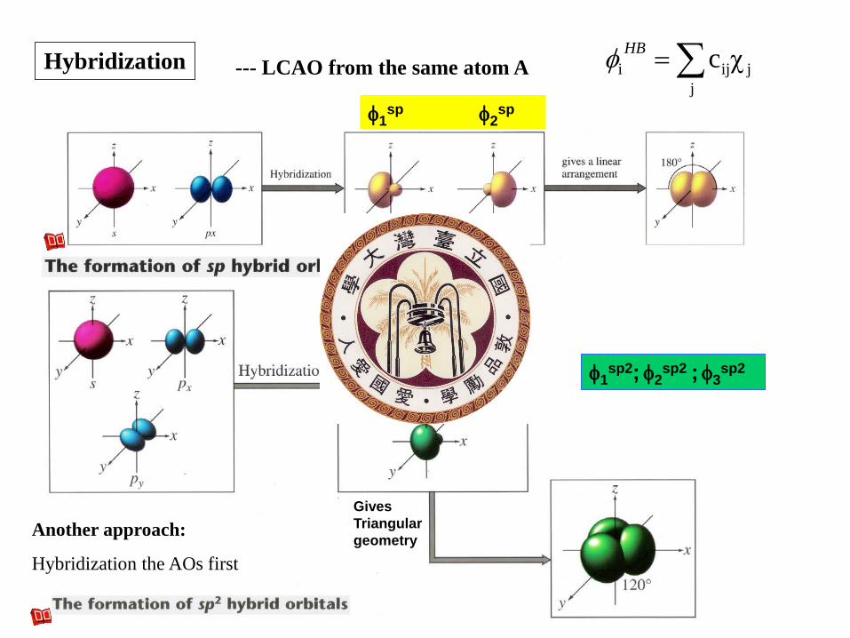
Hybridization --- LCAO from the same atom A ∑=j

jiji χcHBφ

φ1sp φ2

sp

φ1sp2; φ2

sp2 ; φ3sp2

Gives Triangular geometry Another approach:

Hybridization the AOs first

http://www.mhhe.com/physsci/chemistry/essentialchemistry/flash/hybrv18.swf

The Hybrid orbitals動畫網站(英文說明)

The hybrid orbitals for various electron pair arrangments of A

s px py

s px py pz dz2

s p3 dz2 dx2-y2

O

H H

x

z

Recall H2O MOs: Hybridization of the two a1 AOs further stabilized the 1a1 bonding MO.

Applications of Hybridization in MO Theory

2A1+B1+B2 A1+B1 sp-hybridized orbitals

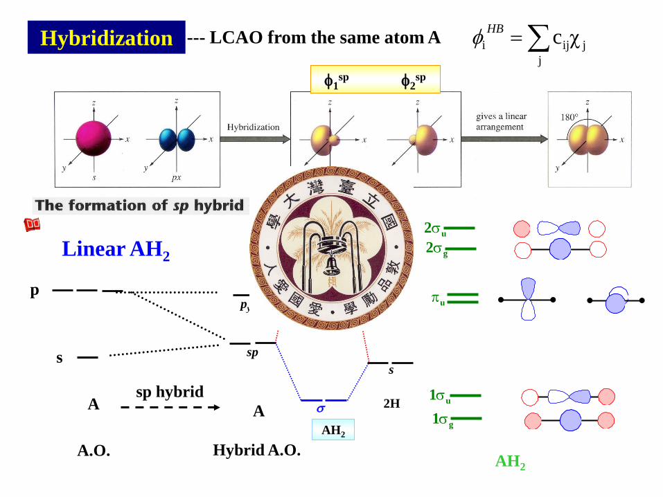
Hybridization --- LCAO from the same atom A ∑=j

jiji χcHBφ

φ1sp φ2

sp

AH2

A 2H

sp

pz

s

σ

σ*

py pz py

A

s

p

sp hybrid

Linear AH2 g2σu2σ

u1σ

g1σ

uπ

AH2 A.O. Hybrid A.O.

Hybridization

∑=j

jiji χcHBφ

φ1sp2; φ2

sp2 ; φ3sp2

--- LCAO from the same atom A

AH2

A 2H

sp2

pz

s σ

σ*

pz Bent AH2

A

s

p

sp2 hybrid

Hybridization

∑=j

jiji χcHBφ

φ1sp2; φ2

sp2 ; φ3sp2

--- LCAO from the same atom A σ*

planar AH3

AH3

A 3H

sp2

pz

s σ

pz

A

s

p

sp2 hybrid

Gives a Triangular geometry

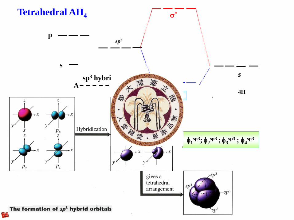
φ1sp3; φ2

sp3 ; φ3sp3 ; φ4

sp3

A 4H

sp3

s A

s

p

sp3 hybrid

AH4

σ

σ* Tetrahedral AH4

Hybrid orbitals of A AL2

linear

bent

BeH2

sp

OH2

D2h E C2(z) C2(y) C2(x) i σ(xy) σ(xz) σ(yz)

Ag 1 1 1 1 1 1 1 1 x2, y2, z2

B1g 1 1 -1 -1 1 1 -1 -1 Rz xy

B2g 1 -1 1 -1 1 -1 1 -1 Ry xz

B3g 1 -1 -1 1 1 -1 -1 1 Rx yz

Au 1 1 1 1 -1 -1 -1 -1

B1u 1 1 -1 -1 -1 -1 1 1 z

B2u 1 -1 1 -1 -1 1 -1 1 y

B3u 1 -1 -1 1 -1 1 1 -1 x

Γ(sp) 2 2 0 0 0 0 2 2 Ag + B1u

C2v E C2 (z) σv(xz) σ’v (yz)

A1 1 1 1 1 z x2, y2, z2

A2 1 1 -1 -1 Rz xy

B1 1 -1 1 -1 x, Ry xz

B2 1 -1 -1 1 y, Rx yz

Γσ 2 0 2 0 A1 + B1 sp; p2

Γt sp3

Γlp 2 0 0 2 A1 + B2 sp; p2

Trick: C∞v (D∞h) symmetry use the C2v (D2h) table

AL3 planar

bent

BH3

sp2; sd2 ; dp2; d3 (s; dz2) ((x,y); (dxy, d x2-y2))

NH3 sd2,, p3; sp2; pd2; d3 (s; ps; dz2) ((x,y); (dxy, d x2-y2); (dxz, dyz))

D3h E 2C3 3C2 σh 2S3 3 σv

A1’ 1 1 1 1 1 1 x2 + y2, z2

A2’ 1 1 -1 1 1 -1 Rz

E’ 2 -1 0 2 -1 0 (x, y) (x2-y2, xy)

A1” 1 1 1 -1 -1 -1

A2” 1 1 -1 -1 -1 1 z

E” 2 -1 0 -2 1 0 (Rx,Ry)

Γ 3 0 1 3 0 1 A1’ + E’

C3v E 2C3 3 σv

A1 1 1 1 z x2 + y2, z2

A2 1 1 -1 Rz

E 2 -1 0 (x,y), (Rx, Ry) (x2-y2, xy), (xz, yz)

Γ 3 0 1 A1 + E

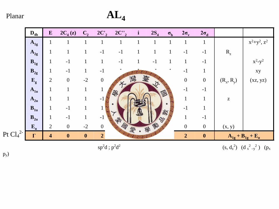
AL4 Planar

Pt Cl42-

sp2d ; p2d2 (s, dz2) (d x2

–y2 ) (px

py)

D4h E 2C4 (z) C2 2C'2 2C''2 i 2S4 σh 2σv 2σd

A1g 1 1 1 1 1 1 1 1 1 1 x2+y2, z2

A2g 1 1 1 -1 -1 1 1 1 -1 -1 Rz

B1g 1 -1 1 1 -1 1 -1 1 1 -1 x2-y2

B2g 1 -1 1 -1 1 1 -1 1 -1 1 xy

Eg 2 0 -2 0 0 2 0 -2 0 0 (Rx, Ry) (xz, yz)

A1u 1 1 1 1 1 -1 -1 -1 -1 -1

A2u 1 1 1 -1 -1 -1 -1 -1 1 1 z

B1u 1 -1 1 1 -1 -1 1 -1 -1 1

B2u 1 -1 1 -1 1 -1 1 -1 1 -1

Eu 2 0 -2 0 0 -2 0 2 0 0 (x, y)

Γ 4 0 0 2 0 0 0 4 2 0 A1g + B1g + Eu

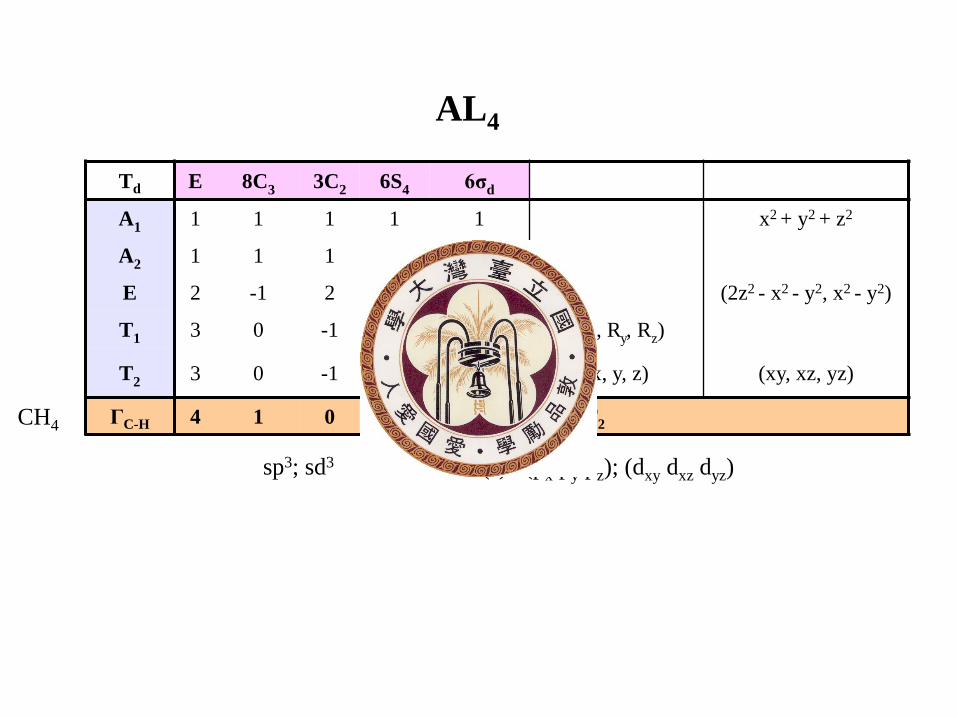
CH4

sp3; sd3 (s) (px py pz); (dxy dxz dyz)

Td E 8C3 3C2 6S4 6σd

A1 1 1 1 1 1 x2 + y2 + z2

A2 1 1 1 -1 -1

E 2 -1 2 0 0 (2z2 - x2 - y2, x2 - y2)

T1 3 0 -1 1 -1 (Rx, Ry, Rz)

T2 3 0 -1 -1 1 (x, y, z) (xy, xz, yz)

ΓC-H 4 1 0 0 2 A1 + T2

AL4

AL5

PF5

sp3d ; spd3 ;

XeBr5

sp3d ; sp2d2 ; sd4

D3h E 2C3 3C2 σh 2S3 3 σv

A1’ 1 1 1 1 1 1 x2 + y2, z2

A2’ 1 1 -1 1 1 -1 Rz

E’ 2 -1 0 2 -1 0 (x, y) (x2-y2, xy)

A1” 1 1 1 -1 -1 -1

A2” 1 1 -1 -1 -1 1 z

E” 2 -1 0 -2 1 0 (Rx,Ry)

Γ 5 2 1 3 0 3 2A1’ + E’ +A2”

C4v E 2C4 C2 2σv 2σd

A1 1 1 1 1 1 z x2 + y2, z2

A2 1 1 1 -1 -1 Rz

B1 1 -1 1 0 -1 x2 - y2

B2 1 -1 1 -1 1 xy

E 2 0 -2 0 0 (x, y), (Rx, Ry) (xz, yz)

Γ 5 1 1 3 1 2A1 + B1 + E

AL6

D4h E 2C4 (z) C2 2C'2 2C''2 i 2S4 σh 2σv 2σd

A1g 1 1 1 1 1 1 1 1 1 1 x2+y2, z2

A2g 1 1 1 -1 -1 1 1 1 -1 -1 Rz

B1g 1 -1 1 1 -1 1 -1 1 1 -1 x2-y2

B2g 1 -1 1 -1 1 1 -1 1 -1 1 xy

Eg 2 0 -2 0 0 2 0 -2 0 0 (Rx, Ry) (xz, yz)

A1u 1 1 1 1 1 -1 -1 -1 -1 -1

A2u 1 1 1 -1 -1 -1 -1 -1 1 1 z

B1u 1 -1 1 1 -1 -1 1 -1 -1 1

B2u 1 -1 1 -1 1 -1 1 -1 1 -1

Eu 2 0 -2 0 0 -2 0 2 0 0 (x, y)

Γeq 4 0 0 2 0 0 0 4 2 0 A1g + B1g + Eu

Γax 2 2 2 0 0 0 0 0 2 0 A1g + A2u

sp3d2

sp2d

pd

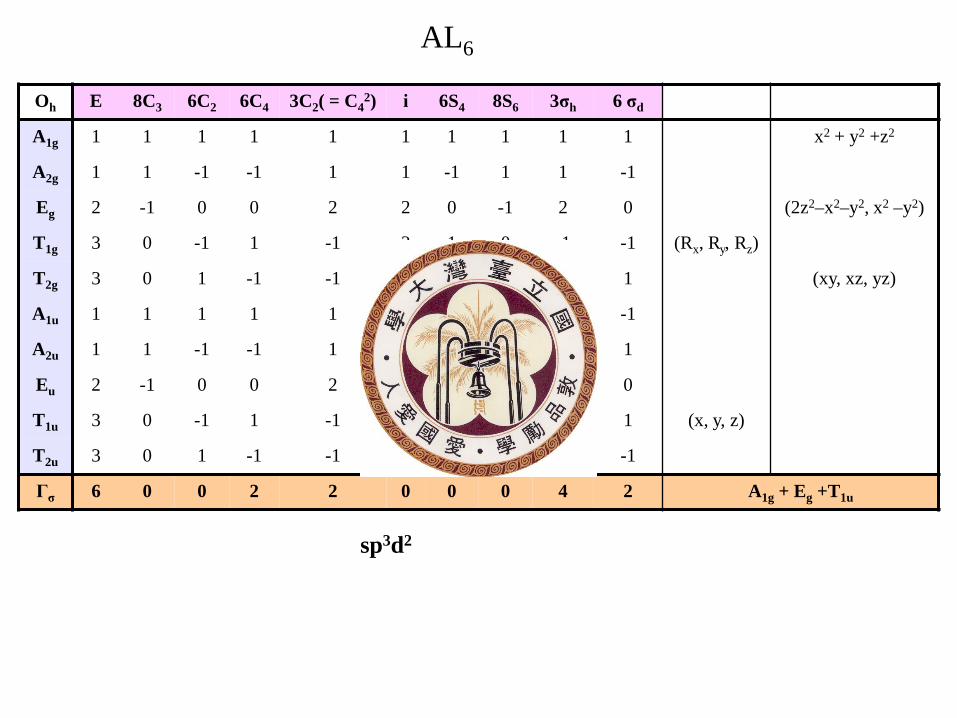
AL6

Oh E 8C3 6C2 6C4 3C2( = C42) i 6S4 8S6 3σh 6 σd

A1g 1 1 1 1 1 1 1 1 1 1 x2 + y2 +z2

A2g 1 1 -1 -1 1 1 -1 1 1 -1

Eg 2 -1 0 0 2 2 0 -1 2 0 (2z2–x2–y2, x2 –y2)

T1g 3 0 -1 1 -1 3 1 0 -1 -1 (Rx, Ry, Rz)

T2g 3 0 1 -1 -1 3 -1 0 -1 1 (xy, xz, yz)

A1u 1 1 1 1 1 -1 -1 -1 -1 -1

A2u 1 1 -1 -1 1 -1 1 -1 -1 1

Eu 2 -1 0 0 2 -2 0 1 -2 0

T1u 3 0 -1 1 -1 -3 -1 0 1 1 (x, y, z)

T2u 3 0 1 -1 -1 -3 1 0 1 -1

Γσ 6 0 0 2 2 0 0 0 4 2 A1g + Eg +T1u

sp3d2

版權聲明 作品 授權條件 作者/來源

© A.W. Potts and W. C. Price, Proc. R. Soc. London, A326, 165 (1972).

© http://wikis.lawrence.edu/display/CHEM/1.2+Molecular+Geometry+Part+II+(Maki+Miura) 2012/05/25 visited

©

http://wps.prenhall.com/wps/media/objects/165/169060/tool0903.gif 2012/05/25 visited

©

http://wps.prenhall.com/wps/media/objects/165/169060/tool0902.gif 2012/05/25 visited

© http://www.chemistry.ucsc.edu/~soliver/151A/Handouts/ 2012/05/25 visited

版權聲明 作品 授權條件 作者/來源

© http://www.chemistry.ucsc.edu/~soliver/151A/Handouts/ 2012/05/25 visited

© http://www.chemistry.ucsc.edu/~soliver/151A/Handouts/ 2012/05/25 visited

©

http://www.chemistry.ucsc.edu/~soliver/151A/Handouts/ 2012/05/25 visited

Yun-Chen Chien

http://en.wikipedia.org/wiki/File:Diborane-2D.png 2012/05/25 visited

版權聲明 作品 授權條件 作者/來源

© Steven S. Zumdahi Chemistry Third Edtion 1993 by D. C. Health and Company

©

Steven S. Zumdahi Chemistry Third Edtion 1993 by D. C. Health and Company

© Steven S. Zumdahi Chemistry Third Edtion 1993 by D. C. Health and Company

©

2006 Brooks / Cole – Thomson

版權聲明 作品 授權條件 作者/來源

© http://universo-diverso.blogspot.com/2007/05/sobre-modelos-moleculares-e-teorias.html 2012/05/26 visited

©

http://universo-diverso.blogspot.com/2007/05/sobre-modelos-moleculares-e-teorias.html 2012/05/26 visited

© http://universo-diverso.blogspot.com/2007/05/sobre-modelos-moleculares-e-teorias.html 2012/05/26 visited

Yun-Chen Chien

版權聲明 作品 授權條件 作者/來源

© http://www.atom.rmutphysics.com/charud/oldnews/0/286/15/25/chemistry/chemical%20bond/bond/bond_files/frame.htm

2012/05/26 visited

© http://www.atom.rmutphysics.com/charud/oldnews/0/286/15/25/chemistry/chemical%20bond/bond/bond_files/frame.htm 2012/05/26 visited

© http://www.nobelprize.org/nobel_prizes/chemistry/laureates/1976/ 2012/05/26 visited

Yun-Chen Chien

Yun-Chen Chien