Occupational Licensing, Labor Mobility, and theUnfairness of Entry Standards

Paolo Buonanno*and Mario Pagliero�

March, 2019

Abstract

Occupational licensing at the local market level often coexists with labor mobil-

ity across local markets. We empirically study a labor market in which a district-

specific entry (licensing) examination is coupled with labor mobility across districts.

Our analysis exploits a change in the grading procedure of the exam, from grading

in the local district to grading in a randomly assigned different district. We doc-

ument that licensing regulation leads to extreme heterogeneity across markets in

admission outcomes (up to 50 percent differences in licensing exam pass rates), un-

fair (discriminatory) admission procedures (up to 49 percent unfair exam results),

and inefficient mobility of workers. We then present a model of occupational li-

censing and labor mobility and test its additional predictions. Our findings provide

the first evidence of regulatory competition based on strategic interaction among

licensing boards.

Keywords: Regulation, labor market regulation, occupational regulation, licensing, legal

market, bar exam.

JEL codes: J08, J44, L84, L50.

*University of Bergamo. E-mail: paolo.buonanno@unibg.it�University of Turin, Collegio Carlo Alberto, and CEPR. E-mail: mario.pagliero@carloalberto.org.

1 Introduction

At present, 22 percent of workers in the EU and 29 percent in the US are required by law

to hold a professional license (Kleiner and Krueger, 2013, Koumenta and Pagliero, 2018).

Entry into licensed professions is typically conditional on educational qualifications and

passing an entry exam, which is often administered by the professional association of the

regulated profession. While this type of regulation may benefit consumers in reducing

asymmetric information (Akerlof, 1970, Leland, 1979), it may also reduce competition

and increase prices, thereby reducing allocative efficiency (Friedman and Kuznets, 1954,

Smith, 1776).

Most licensed markets are characterized by regulation at the local market level and la-

bor mobility across markets. In the EU, hundreds of professions are licensed in accordance

with country-specific local laws. At the same time, mobility of workers across countries

is one of the cornerstones of the EU treaty. For example, physicians, nurses, archi-

tects, dentists and veterinaries are subject to country-specific entry exams and automatic

recognition of their professional titles across EU member states. Lawyers, accountants,

electricians, plumbers and many other professions are similarly subject to country-specific

entry exams, and their mobility is regulated by country-specific regulations and EU direc-

tives. Given the importance of this subject, harmonization of requirements and mutual

recognition of professional licensing qualifications is high on the policy agenda in the EU.

Also in the US, state licensing regulations for many professions coexist with the gen-

eral principle of labor mobility across states.1 For example, nurses can pass the entry

exam and then move within a large number of states (the nurse licensure compact). Af-

ter passing the state bar exam, lawyers can move on the basis of bilateral agreements

among states. Teachers, dentists and many other professions can also move across states

subject to recognition of their state credentials.2 Occupational licensing regulations are

1State-based licensing requirements make it difficult for workers to practice across state lines. Thiscreates the need for mutual licensing-recognition agreements, so that workers can relocate without havingto requalify.

2In the US, occupational licensing is becoming an important and bipartisan topic in the policy debate.For example, in 2015, a report published by the Obama White House (White House, 2015) called for areview of the costs and benefits of occupational licensing regulations. In July 2017, Alexander Acosta,

2

also important as they are subject to antitrust scrutiny. In the US, the Federal Trade

Commission has been particularly active in applying antitrust legislation to occupational

licensing boards.3 This paper shows that the combination of occupational regulation at

the local market level and labor mobility may generate extreme heterogeneity across mar-

kets in admission outcomes, unfair (discriminatory) admission procedures, and inefficient

mobility of workers.

While anecdotal evidence of the importance of the combination of local occupational

regulation and labor mobility is abundant, there is a lack of studies (theoretical or em-

pirical) on its effects. One reason is that heterogeneity of labor market regulation across

countries makes it difficult to compare labor markets.4 In this paper, we focus on one

specific labor market in one specific country: the Italian market for lawyers. This market

features a combination of local entry regulation and labor mobility across local markets.

Moreover, each local market follows the same rules and procedures for admission, making

comparison of entry standards particularly easy. Finally, the Italian market for lawyers

is homogeneous across local markets in terms of their legal framework, labor market

regulations, and language.

The Italian bar exam consists of a written and an oral component. Exams are admin-

istered in each of 26 districts and exactly the same written questions are used all over

country. However, grading standards may vary significantly across districts, since local

professional associations are responsible for grading the exams. After passing the bar

exam, newly licensed lawyers are free to move across districts and practice wherever they

choose. This generates heterogeneity in entry barriers and labor mobility across local

markets.5

US Secretary of labor of the Trump administration, also recommended a thorough review of occupationallicensing regulations.

3In the 2015 North Carolina Board of Dental Examiners v. Federal Trade Commission case, theU.S. Supreme Court determined that state licensing boards controlled by market participants and notdirectly supervised by the state are not immune from federal antitrust scrutiny. For a summary of recentdevelopments in antitrust enforcement in this area, see Stutz (2017) and Kwoka et al. (2019).

4 For example, bilateral agreements across states are very heterogeneous and difficult to study sys-tematically.

5Although the differences in entry barriers are large, they are limited to differences in the severity ofgrading procedures.

3

In the early 2000s, the differences in pass rates across districts in the Italian market

for lawyers raised concerns about the fairness of the bar exam. In 2003, the rules for

grading the exam changed. Starting with the 2004 examination, the written exams were

no longer graded locally, but sent to a different district, randomly assigned each year

after administration of the exam. This is not only an interesting and unusual policy

experiment, but the randomization of the grading district also provides a convenient

source of variation that can be used to separately identify the severity of the grading

standards (the source of differences in entry barriers across districts) from differences in

the quality of candidates.

Exploiting data on the Italian bar exam between 1998 and 2012, we document the

existence of extreme heterogeneity across markets in exam pass rates, which vary between

16 and 96 percent. In particular, wealthier districts systematically have lower pass rates.

We show that these differences are mainly caused by large and unfair (discriminatory)

differences in grading standards, with identical exam candidates treated differently from

district to district. We estimate that up to 49 percent of candidates experienced an

unfair exam outcome.6 These differences in grading standards lead to inefficient mobility

of workers from poorer to richer districts. A 10 percent increase in the pass rate (due

to a decrease in grading standards) leads to a 39 percent increase in net out-migration

(number of successful candidates in the local bar exam - number of newly registered

lawyers in the district).

We show that these results are consistent with a model of the incentives provided

by regulation and that strategic interaction between local professional associations can

explain the observed heterogeneity across districts. As workers try to arbitrage differences

in work amenities across markets, local professional associations lose control of the labor

supply in their own market. In such a context, the entry requirements in one market have

consequences in other markets, thus forcing professional associations to interact with

one another in setting entry requirements. The model shows that competition among

6In the sense that they either passed the exam despite performing worse than some other candidatewho failed in a different district, or they failed the exam despite performing better than some othercandidate who passed in a different district.

4

licensing boards leads to heterogeneity in admission standards (with higher standards in

richer markets), unfair exams, and inefficient mobility. The model can also rationalize

the implementation of the 2003 reform, which reduced the differences between rich and

poor districts, yet increased the average difficulty of the exam. The model also provides

other predictions, which are then tested with the data. Finally, we show some evidence

from the US market for lawyers that is consistent with the main predictions of the model

and our empirical findings. This suggests that our results are potentially relevant in other

contexts.

A long and distinguished literature studies the effects of occupational licensing (see

Kleiner, 2000, for a review) on prices, mobility (Federman et al., 2006, Holen, 1965), and

the quality of the goods and services provided in licensed markets (Angrist and Guryan,

2004, Kleiner and Kudrle, 2000, Larsen, 2013, Maurizi, 1974). A more recent literature

has started to investigate the behavior of licensing boards, and attempts to document

how entry regulations, restrictions to mobility, and the list of activities reserved to each

profession are determined.7

The paper is organized as follows. Section 2 describes the Italian market for lawyers

and provides some preliminary evidence on exam outcomes. Section 3 exploits the ran-

domization introduced by the 2003 reform to show that grading standards differ across

districts. Section 4 introduces an empirical model that allows to separately identify

differences in grading standards and candidates’ quality. The consequences of different

grading standards on exam outcomes and fairness are described in Section 5. Section 6

investigates the mechanism that generates the observed differences in grading standards,

presents the model, and tests its predictions.

7See for example Kleiner et al. (2016), Pagliero (2011, 2013).

5

2 Occupational licensing in the Italian market for

lawyers

Italian lawyers are a typical licensed profession. Lawyers must be registered in the official

register that is maintained by a local bar association, to which the national law gives

extensive legal prerogatives. The bar associations, which are formed by all the lawyers

listed in the official register, elect a council and a chairman. The latter are legally

responsible for the official register and, more generally, for the professional conduct of

their associates. They also settle disputes among lawyers, or between lawyers and their

clients, and hold some disciplinary authority, such as suspending or expelling lawyers

from the official register.

The national law also regulates the criteria for entry into the profession. Aspiring

lawyers must complete a university degree in law (5 years) followed by a two-year ap-

prenticeship in a law office, where they work with an experienced lawyer. They must

then pass the bar exam, which takes approximately one year to complete. Candidates

are allowed to take the exam only in the district in which they are registered and do

their apprenticeship.8 The bar exam consists of a written and an oral component. Access

to the oral exam is conditional on passing the written exam. The written exam is held

annually, usually in December, in each of the 26 district appeal courts.9 The written

exam takes place simultaneously in each district and the same exam questions are used

throughout the country. Conditional on passing the written exam, candidates then take

the oral exam, usually in the Autumn of the following year, in the same district.

Before 2004, the written exam was graded in the district where the candidate took the

exam. Although exam questions were identical, grading was performed by local grading

committees composed of lawyers, judges, and law professors working in the district. As

8This is to discourage mobility of exam candidates and limit arbitrage opportunities across examsin different districts. Since 2003, to further discourage mobility, trainees moving to a different districtduring the training period are required to take the exam in the district in which they have done most oftheir training.

9There is generally one destrict appeal court for each Italian region, although Lombardy has two (Bres-cia and Milano), Campania two (Napoli and Salerno), Calabria two (Catanzaro and Reggio Calabria),Puglia two (Bari and Lecce), and Sicily four (Caltanissetta, Catania, Messina and Palermo)

6

of 2004, new regulations came into force.10 Each year, districts are partitioned by the

Ministry of Justice into groups of 3 to 8 districts. Groups vary every year in size and

composition, but they tend to include districts with similar number of applicants. The

grading committee in each district is then assigned to grade the essays coming from

another district, randomly drawn from the same group.11 The reform only affected the

procedure for grading of the written exam. Candidates still take the oral exam in the

district where the written exam was taken.

After passing the oral exam, licensed lawyers are free to register and practice in the

local bar association of their choice. Therefore, although local licensing exams play a

key role in admission procedures, the labor market for lawyers is a national one. This

is the result of the evolution of the legal profession after Italy was unified in the 19th

century. While a common labor market was created, the pre-existing heterogeneity in

institutions and legal traditions persisted in the form of local bar examinations.12 The

2004 reform was motivated by the perceived unfairness of the existing procedures, which

allegedly resulted in systematic differences in pass rates across districts. Following an

intense debate, the grading procedures were eventually changed.

2.1 The data and preliminary evidence

We collected data on the number of participants and successful candidates in the written

and oral exams for each district from 1998 to 2012.13 This data provides information on

the pass rates for the written and oral examinations, as well as the overall pass rate (i.e.,

the percentage of candidates who pass both stages). We complement this with data on

the number of lawyers in each district and year from administrative records.14 Economic

10The so called Castelli reform, Law 180/2003, http://www.camera.it/parlam/leggi/03180l.htm11The number of graders in each district depends on the number of candidates in that district, hence

the law requires to group districts with similar number of candidates to avoid excessive workloads ongraders.

12See Tacchi (2002) for a detailed history of the legal profession in Italy.13Ministry of Justice, https://www.giustizia.it/giustizia/it/mg_12_1_2_3_2.wp. The city of

Bolzano is excluded from the sample as it is subject to different rules. Since candidates can take theexam in German as well as in Italian, they are always graded by a local committee

14The Social Security Office (Cassa Nazionale Forense) provides data on the number of lawyers ineach local register.

7

and demographic variables (population density, real GDP per capita, unemployment rate)

at the district level over the same period were obtained from the National Institute of

Statistics (ISTAT ).

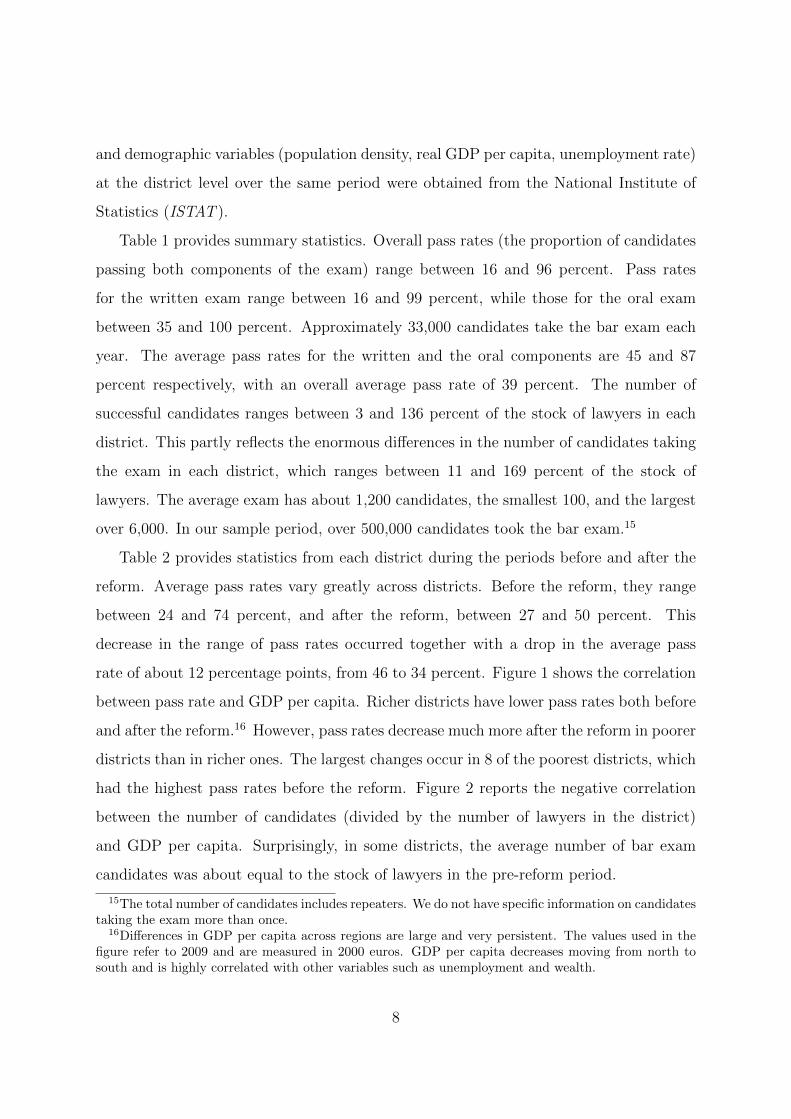
Table 1 provides summary statistics. Overall pass rates (the proportion of candidates

passing both components of the exam) range between 16 and 96 percent. Pass rates

for the written exam range between 16 and 99 percent, while those for the oral exam

between 35 and 100 percent. Approximately 33,000 candidates take the bar exam each

year. The average pass rates for the written and the oral components are 45 and 87

percent respectively, with an overall average pass rate of 39 percent. The number of

successful candidates ranges between 3 and 136 percent of the stock of lawyers in each

district. This partly reflects the enormous differences in the number of candidates taking

the exam in each district, which ranges between 11 and 169 percent of the stock of

lawyers. The average exam has about 1,200 candidates, the smallest 100, and the largest

over 6,000. In our sample period, over 500,000 candidates took the bar exam.15

Table 2 provides statistics from each district during the periods before and after the

reform. Average pass rates vary greatly across districts. Before the reform, they range

between 24 and 74 percent, and after the reform, between 27 and 50 percent. This

decrease in the range of pass rates occurred together with a drop in the average pass

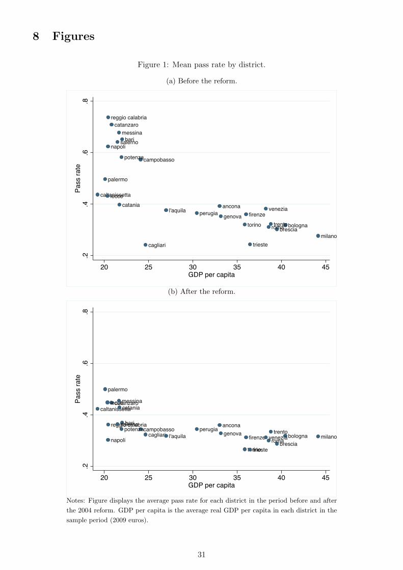
rate of about 12 percentage points, from 46 to 34 percent. Figure 1 shows the correlation

between pass rate and GDP per capita. Richer districts have lower pass rates both before

and after the reform.16 However, pass rates decrease much more after the reform in poorer

districts than in richer ones. The largest changes occur in 8 of the poorest districts, which

had the highest pass rates before the reform. Figure 2 reports the negative correlation

between the number of candidates (divided by the number of lawyers in the district)

and GDP per capita. Surprisingly, in some districts, the average number of bar exam

candidates was about equal to the stock of lawyers in the pre-reform period.

15The total number of candidates includes repeaters. We do not have specific information on candidatestaking the exam more than once.

16Differences in GDP per capita across regions are large and very persistent. The values used in thefigure refer to 2009 and are measured in 2000 euros. GDP per capita decreases moving from north tosouth and is highly correlated with other variables such as unemployment and wealth.

8

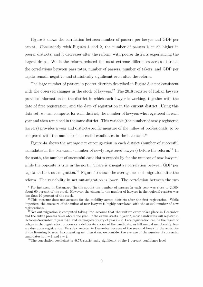
Figure 3 shows the correlation between number of passers per lawyer and GDP per

capita. Consistently with Figures 1 and 2, the number of passers is much higher in

poorer districts, and it decreases after the reform, with poorer districts experiencing the

largest drops. While the reform reduced the most extreme differences across districts,

the correlations between pass rates, number of passers, number of takers, and GDP per

capita remain negative and statistically significant even after the reform.

The large number of passers in poorer districts described in Figure 3 is not consistent

with the observed changes in the stock of lawyers.17 The 2018 register of Italian lawyers

provides information on the district in which each lawyer is working, together with the

date of first registration, and the date of registration in the current district. Using this

data set, we can compute, for each district, the number of lawyers who registered in each

year and then remained in the same district. This variable (the number of newly registered

lawyers) provides a year and district-specific measure of the inflow of professionals, to be

compared with the number of successful candidates in the bar exam.18

Figure 4a shows the average net out-migration in each district (number of successful

candidates in the bar exam - number of newly registered lawyers) before the reform.19 In

the south, the number of successful candidates exceeds by far the number of new lawyers,

while the opposite is true in the north. There is a negative correlation between GDP per

capita and net out-migration.20 Figure 4b shows the average net out-migration after the

reform. The variability in net out-migration is lower. The correlation between the two

17For instance, in Catanzaro (in the south) the number of passers in each year was close to 2,000,about 60 percent of the stock. However, the change in the number of lawyers in the regional register wasless than 10 percent of the stock.

18This measure does not account for the mobility across districts after the first registration. Whileimperfect, this measure of the inflow of new lawyers is highly correlated with the actual number of newregistrations.

19Net out-migration is computed taking into account that the written exam takes place in Decemberand the entire process takes about one year. If the exams starts in year t, most candidates will register inOctober-November of year t+1 and January-February of year t+2. Late registration can be the result ofdelays in the registration process or a deliberate choice of the candidate, as full annual membership feesare due upon registration. Very few register in December because of the seasonal break in the activitiesof the licensing boards. In computing net migration, we consider the average of the number of successfulcandidates in t− 1 and t− 2.

20The correlation coefficient is -0.57, statistically significant at the 1 percent confidence level.

9

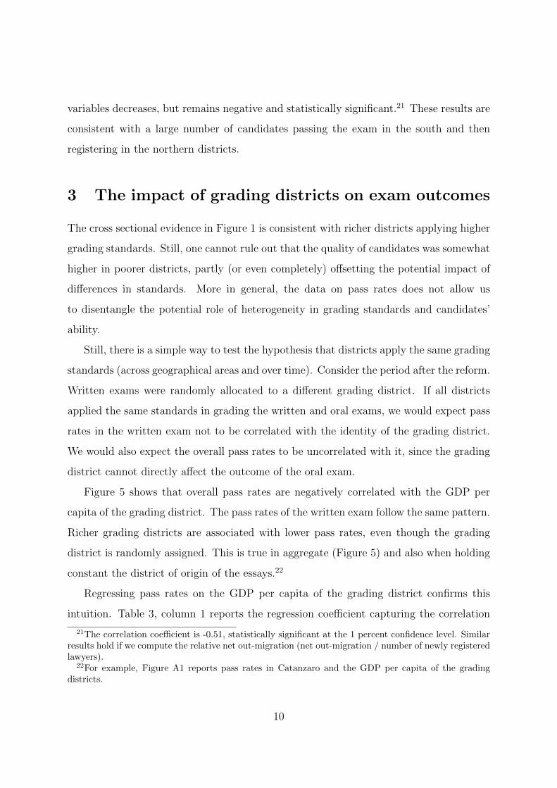
variables decreases, but remains negative and statistically significant.21 These results are

consistent with a large number of candidates passing the exam in the south and then

registering in the northern districts.

3 The impact of grading districts on exam outcomes

The cross sectional evidence in Figure 1 is consistent with richer districts applying higher

grading standards. Still, one cannot rule out that the quality of candidates was somewhat

higher in poorer districts, partly (or even completely) offsetting the potential impact of

differences in standards. More in general, the data on pass rates does not allow us

to disentangle the potential role of heterogeneity in grading standards and candidates’

ability.

Still, there is a simple way to test the hypothesis that districts apply the same grading

standards (across geographical areas and over time). Consider the period after the reform.

Written exams were randomly allocated to a different grading district. If all districts

applied the same standards in grading the written and oral exams, we would expect pass

rates in the written exam not to be correlated with the identity of the grading district.

We would also expect the overall pass rates to be uncorrelated with it, since the grading

district cannot directly affect the outcome of the oral exam.

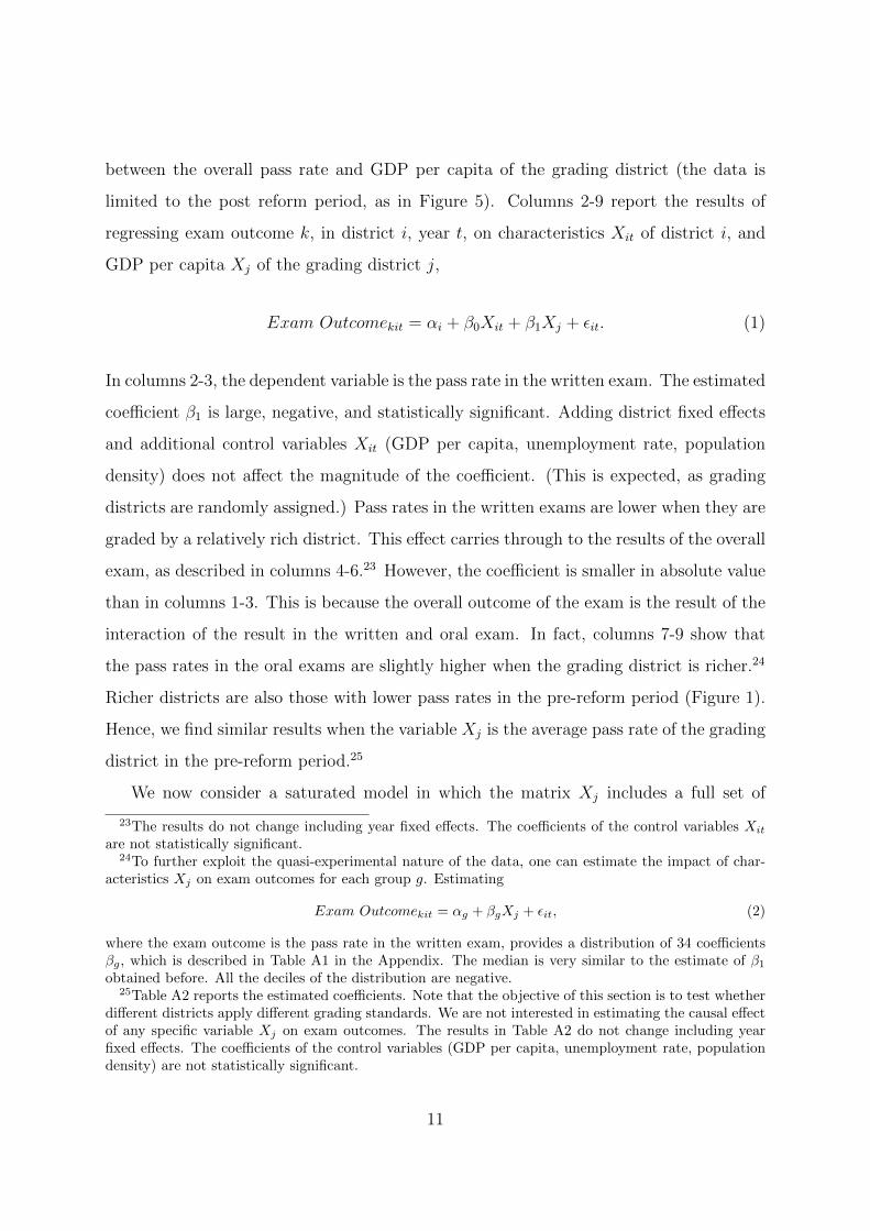
Figure 5 shows that overall pass rates are negatively correlated with the GDP per

capita of the grading district. The pass rates of the written exam follow the same pattern.

Richer grading districts are associated with lower pass rates, even though the grading

district is randomly assigned. This is true in aggregate (Figure 5) and also when holding

constant the district of origin of the essays.22

Regressing pass rates on the GDP per capita of the grading district confirms this

intuition. Table 3, column 1 reports the regression coefficient capturing the correlation

21The correlation coefficient is -0.51, statistically significant at the 1 percent confidence level. Similarresults hold if we compute the relative net out-migration (net out-migration / number of newly registeredlawyers).

22For example, Figure A1 reports pass rates in Catanzaro and the GDP per capita of the gradingdistricts.

10

between the overall pass rate and GDP per capita of the grading district (the data is

limited to the post reform period, as in Figure 5). Columns 2-9 report the results of

regressing exam outcome k, in district i, year t, on characteristics Xit of district i, and

GDP per capita Xj of the grading district j,

Exam Outcomekit = αi + β0Xit + β1Xj + εit. (1)

In columns 2-3, the dependent variable is the pass rate in the written exam. The estimated

coefficient β1 is large, negative, and statistically significant. Adding district fixed effects

and additional control variables Xit (GDP per capita, unemployment rate, population

density) does not affect the magnitude of the coefficient. (This is expected, as grading

districts are randomly assigned.) Pass rates in the written exams are lower when they are

graded by a relatively rich district. This effect carries through to the results of the overall

exam, as described in columns 4-6.23 However, the coefficient is smaller in absolute value

than in columns 1-3. This is because the overall outcome of the exam is the result of the

interaction of the result in the written and oral exam. In fact, columns 7-9 show that

the pass rates in the oral exams are slightly higher when the grading district is richer.24

Richer districts are also those with lower pass rates in the pre-reform period (Figure 1).

Hence, we find similar results when the variable Xj is the average pass rate of the grading

district in the pre-reform period.25

We now consider a saturated model in which the matrix Xj includes a full set of

23The results do not change including year fixed effects. The coefficients of the control variables Xit

are not statistically significant.24To further exploit the quasi-experimental nature of the data, one can estimate the impact of char-

acteristics Xj on exam outcomes for each group g. Estimating

Exam Outcomekit = αg + βgXj + εit, (2)

where the exam outcome is the pass rate in the written exam, provides a distribution of 34 coefficientsβg, which is described in Table A1 in the Appendix. The median is very similar to the estimate of β1obtained before. All the deciles of the distribution are negative.

25Table A2 reports the estimated coefficients. Note that the objective of this section is to test whetherdifferent districts apply different grading standards. We are not interested in estimating the causal effectof any specific variable Xj on exam outcomes. The results in Table A2 do not change including yearfixed effects. The coefficients of the control variables (GDP per capita, unemployment rate, populationdensity) are not statistically significant.

11

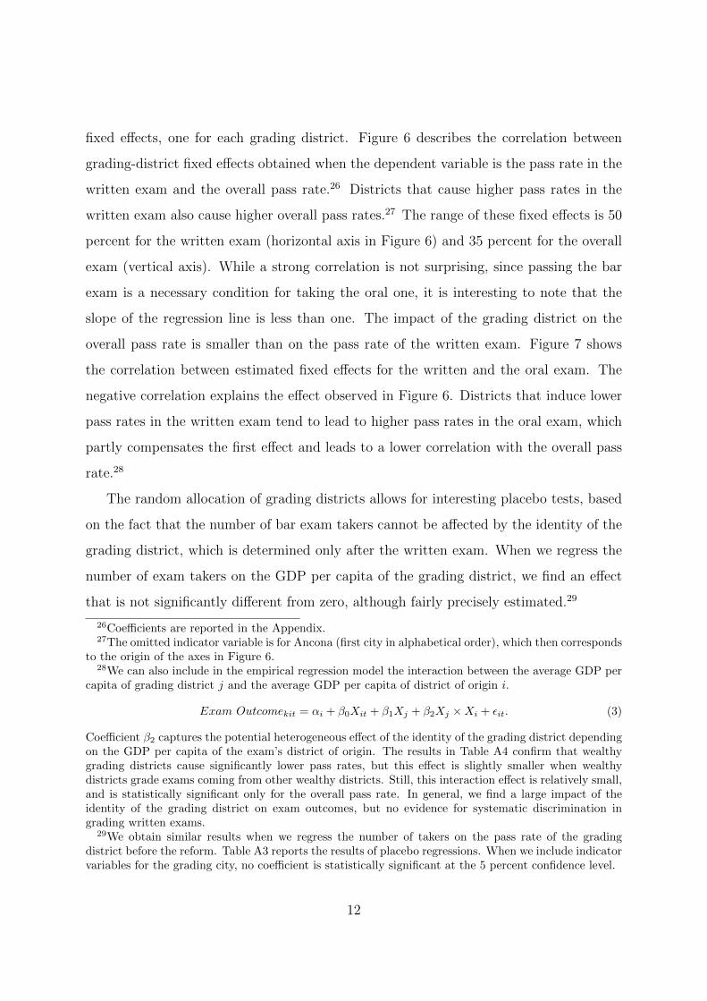
fixed effects, one for each grading district. Figure 6 describes the correlation between

grading-district fixed effects obtained when the dependent variable is the pass rate in the

written exam and the overall pass rate.26 Districts that cause higher pass rates in the

written exam also cause higher overall pass rates.27 The range of these fixed effects is 50

percent for the written exam (horizontal axis in Figure 6) and 35 percent for the overall

exam (vertical axis). While a strong correlation is not surprising, since passing the bar

exam is a necessary condition for taking the oral one, it is interesting to note that the

slope of the regression line is less than one. The impact of the grading district on the

overall pass rate is smaller than on the pass rate of the written exam. Figure 7 shows

the correlation between estimated fixed effects for the written and the oral exam. The

negative correlation explains the effect observed in Figure 6. Districts that induce lower

pass rates in the written exam tend to lead to higher pass rates in the oral exam, which

partly compensates the first effect and leads to a lower correlation with the overall pass

rate.28

The random allocation of grading districts allows for interesting placebo tests, based

on the fact that the number of bar exam takers cannot be affected by the identity of the

grading district, which is determined only after the written exam. When we regress the

number of exam takers on the GDP per capita of the grading district, we find an effect

that is not significantly different from zero, although fairly precisely estimated.29

26Coefficients are reported in the Appendix.27The omitted indicator variable is for Ancona (first city in alphabetical order), which then corresponds

to the origin of the axes in Figure 6.28We can also include in the empirical regression model the interaction between the average GDP per

capita of grading district j and the average GDP per capita of district of origin i.

Exam Outcomekit = αi + β0Xit + β1Xj + β2Xj ×Xi + εit. (3)

Coefficient β2 captures the potential heterogeneous effect of the identity of the grading district dependingon the GDP per capita of the exam’s district of origin. The results in Table A4 confirm that wealthygrading districts cause significantly lower pass rates, but this effect is slightly smaller when wealthydistricts grade exams coming from other wealthy districts. Still, this interaction effect is relatively small,and is statistically significant only for the overall pass rate. In general, we find a large impact of theidentity of the grading district on exam outcomes, but no evidence for systematic discrimination ingrading written exams.

29We obtain similar results when we regress the number of takers on the pass rate of the gradingdistrict before the reform. Table A3 reports the results of placebo regressions. When we include indicatorvariables for the grading city, no coefficient is statistically significant at the 5 percent confidence level.

12

Taken together, these results provide 3 main insights. First, not all districts apply the

same grading standards. Second, the estimated impact of the grading district is extremely

heterogeneous. Third, the impact of the grading district is not limited to the results of

the written exam. Pass rates in the oral exam are also affected, although in the opposite

direction. This may be because a more selective written exam leads to a better pool of

candidates at the oral exam, which may then lead to higher pass rates. Such a selection

mechanism requires correlation of candidates’ ability in the written and oral exams. It

is also possible that licensing boards react to higher grading standards in the written

exam by decreasing grading standards in the oral. To further explore these hypotheses,

we need to define more precisely how candidates’ ability and grading standards interact

to determine pass rates. This is the topic of the next section.

4 Identification of grading standards

In this section, we introduce a model that links grading standards, candidate quality, and

exam outcomes. In this setting, data on pass rates and the randomization of the grading

district separately identify grading standards and candidate quality. We start by modeling

how differences in (unobserved) candidates’ ability across districts generate differences in

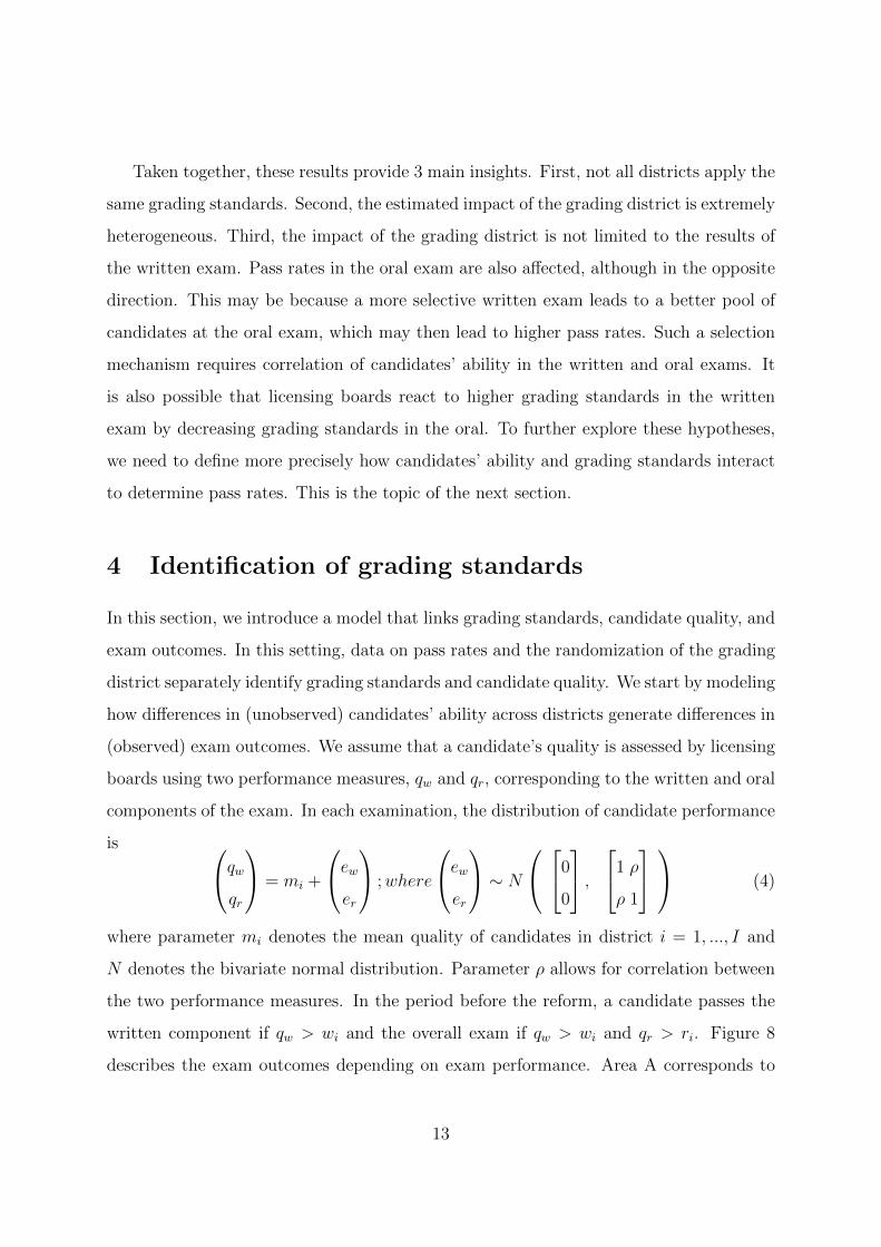
(observed) exam outcomes. We assume that a candidate’s quality is assessed by licensing

boards using two performance measures, qw and qr, corresponding to the written and oral

components of the exam. In each examination, the distribution of candidate performance

is qwqr

= mi +

ewer

;where

ewer

∼ N

0

0

,1 ρ

ρ 1

(4)

where parameter mi denotes the mean quality of candidates in district i = 1, ..., I and

N denotes the bivariate normal distribution. Parameter ρ allows for correlation between

the two performance measures. In the period before the reform, a candidate passes the

written component if qw > wi and the overall exam if qw > wi and qr > ri. Figure 8

describes the exam outcomes depending on exam performance. Area A corresponds to

13

candidates failing the written exam, area B corresponds to candidates passing the written

exam but failing the oral, and area C corresponds to candidates passing both components

of the exam.

In the period after the reform, the written exam in district i is graded by district j, so

that a candidate passes the written exam if qw > w′j and the overall exam if qw > w′j and

qr > r′i, where w′j and r′i denote the exam thresholds after the reform. If it is not possible

to partition districts into subsets that grade exams independently (as it is the case in our

data), then the parameters mi, wi, w′i, ri, r

′i, and ρ are identified (after normalizing the

mean quality of candidates in one district, m1 = 0).30

The parameters are identified jointly by the pass rates, the randomization of the

grading district, and the functional form of the performance distribution. The intuition

is that, given the normalization m1 = 0, pass rate data identify the exam thresholds in

district 1. Then, the repeated randomization of the grading district sequentially identifies

the thresholds and the mean quality in the other districts. The remaining parameter ρ

is identified by the functional form assumption.

The model allows for different grading standards in each district before and after

the reform. In general, we expect wi to be different from w′i, as a result of the different

environment in which licensing boards operate.31 Still, the model places some restrictions

on their behavior. In particular, the parameters wi and ri (w′i and r′i) are assumed to

be constant during the years before (after) the reform. Hence, the model captures the

average licensing board behavior before and after the reform, but not the transition

process or the year-to-year variability in exam difficulty.32

30The proof is reported in Appendix B. We observe the outcomes of the randomization for many years.This information can be summarized by a matrix that links the grading district to the district in whichthe written exam took place. This matrix describes a connected graph in which it is not possible topartition districts into subsets that grade exams independently.

31The reform may affect licensing boards incentives. This is because wi is used to grade written examscoming from district i, w′i is used to grade written exams from another district randomly matched withi. Similarly, we expect ri to be different from r′i. Before the reform the grading standard ri is set inconjunction with wi, while after the reform the pass rate of the written exam is determined by thegrading standard of another district.

32The assumption that r′i is fixed within the period after the reform implies that district i cannot reactto the year-to-year variability in the identity of the grading district j. While this assumption is somewhatrestrictive, procedures for evaluating oral exams and selecting examiners cannot be easily changed on

14

A potentially more restrictive assumption is that the quality mi is time invariant.

It is possible that the reform affected the mean quality of candidates in each district.

Although mobility of bar exam candidates is limited (due to the rules applying to the

two-year apprenticeship period), the same pool of exam candidates may sort differently

across districts as a consequence of the new standards w′i and r′i. If we allowed for

arbitrary values of quality before (mi) and after (m′i) the reform, then only m′i, w′i, r

′i,

and ρ would be identified, since there is no randomization in the pre-reform period. Most

of the empirical analysis would still be possible in this case (and our results would not

change), but we would not be able to assess the impact of the reform.

However, it is possible to allow for the endogeneity of candidates’ quality. Consider

the case in which the quality of candidates is a linear function of exam difficulty,

mi = µi + ϕ1ri + ϕ2wi, (5)

before the reform, and

m′i = µi + ϕ1r′i + ϕ2E(w′−i), (6)

after the reform, where E(w′−i) denotes the expected threshold in the written exam

for candidates taking the exam in district i.33 If the mean and variance of the quality

distribution of bar exam candidates at the national level is stable, then the parameters w′i,

r′i, wi, ri, ρ, and (µi, ϕ1, ϕ2) are identified. (Appendix B provides details on identification.)

4.1 Estimation

We estimate the parameters of the model by maximum likelihood. The contribution to

the likelihood of one observation in our data set (one examination in one specific district)

a yearly basis. Moreover, while the reform was a major change that could change the long-run flow ofnew lawyers in the market, the random year-to-year variability in the grading standards w used by otherdistricts is unlikely to affect the long-run flow of new entrants into the profession.

33Written exams are graded by some random district other than i. Candidates do not know the gradingdistrict or the group assignment before taking the exam.

15

is

L1 =∏

Pr(qw < w,mi)n1Pr(qw > w, qr < r,mi)

n2Pr(qw > w, qr > r,mi)n3 (7)

where n1 is the number of candidates failing the written exam, n2 the number of candi-

dates passing the written exam but failing the oral, and n3 is the number of candidates

passing both components. We estimate the results for two empirical specifications. The

first assumes that quality is constant, mi = µi. The second assumes that the mean qual-

ity of candidates before and after the reform is given by (5) and (6) respectively, with the

normalization µ1 = 0. Since the results do not vary depending on the specification used,

we will report the results of the second, more general, specification.34

5 Empirical results on admission standards and exam

fairness

5.1 The heterogeneity of admission standards

Table A5 in Appendix A reports the estimation results. The correlation in candidate

ability in the written and oral components of the bar exam is positive and precisely

estimated (ρ = 0.438). ϕ1 and ϕ2 in equation (4) are positive, but small and not sig-

nificantly different from zero.35 Figure 9 reports the estimated threshold w before and

after the reform for each district, ordered by their GDP per capita. Before the reform,

the threshold w is significantly higher in richer districts than in poorer districts. After

the reform, this correlation is much smaller, as poorer districts adopt higher standards,

while richer districts do not substantially change their thresholds. Figure 10 shows the

34Other specifications are possible, but the small differences between the results obtained using thesetwo specifications suggest that changes in the functional form used to control for the possible endogeneityof quality do not lead to significant changes in the results.

35The mean quality of candidates (mi and m′i) varies between -0.30 and 0.16 standard deviationsbefore the reform, and slightly less after the reform. Before the reform, the estimated grading standardw varies between -1.19 and 0.58 standard deviations, with a range of 1.77 standard deviations. Thegrading standard for the oral exam (r) varies between -2.09 and -0.20, with a range of 1.89 standarddeviations.

16

change in grading standards in written exams and GDP per capita.36 These correlations

imply that the reform harmonized the expected grading standard of the written exam.

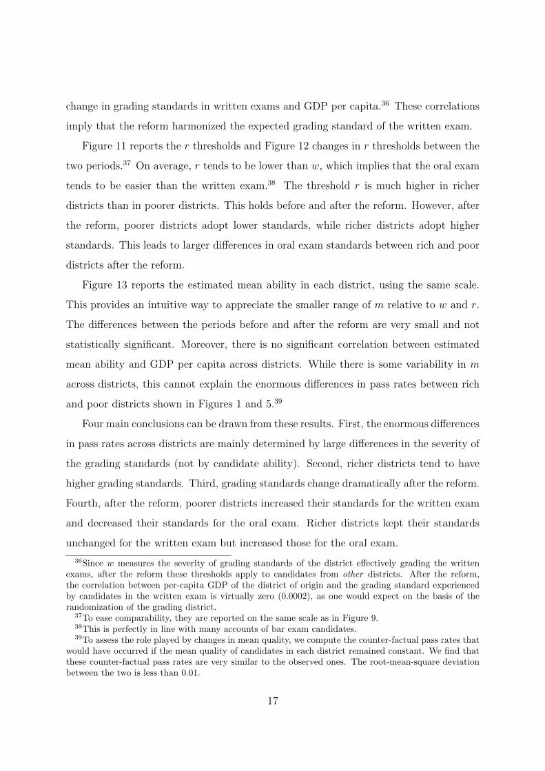
Figure 11 reports the r thresholds and Figure 12 changes in r thresholds between the

two periods.37 On average, r tends to be lower than w, which implies that the oral exam

tends to be easier than the written exam.38 The threshold r is much higher in richer

districts than in poorer districts. This holds before and after the reform. However, after

the reform, poorer districts adopt lower standards, while richer districts adopt higher

standards. This leads to larger differences in oral exam standards between rich and poor

districts after the reform.

Figure 13 reports the estimated mean ability in each district, using the same scale.

This provides an intuitive way to appreciate the smaller range of m relative to w and r.

The differences between the periods before and after the reform are very small and not

statistically significant. Moreover, there is no significant correlation between estimated

mean ability and GDP per capita across districts. While there is some variability in m

across districts, this cannot explain the enormous differences in pass rates between rich

and poor districts shown in Figures 1 and 5.39

Four main conclusions can be drawn from these results. First, the enormous differences

in pass rates across districts are mainly determined by large differences in the severity of

the grading standards (not by candidate ability). Second, richer districts tend to have

higher grading standards. Third, grading standards change dramatically after the reform.

Fourth, after the reform, poorer districts increased their standards for the written exam

and decreased their standards for the oral exam. Richer districts kept their standards

unchanged for the written exam but increased those for the oral exam.

36Since w measures the severity of grading standards of the district effectively grading the writtenexams, after the reform these thresholds apply to candidates from other districts. After the reform,the correlation between per-capita GDP of the district of origin and the grading standard experiencedby candidates in the written exam is virtually zero (0.0002), as one would expect on the basis of therandomization of the grading district.

37To ease comparability, they are reported on the same scale as in Figure 9.38This is perfectly in line with many accounts of bar exam candidates.39To assess the role played by changes in mean quality, we compute the counter-factual pass rates that

would have occurred if the mean quality of candidates in each district remained constant. We find thatthese counter-factual pass rates are very similar to the observed ones. The root-mean-square deviationbetween the two is less than 0.01.

17

These results are in line with the reduced form results reported in Section 3. Moreover,

the results imply that both selection and strategic behavior play a role in determining

the impact on pass rates. In fact, richer grading districts tend to exclude the worse

candidates from the oral exam (selection), since candidate quality at the written and oral

exam are highly correlated. Moreover, poorer districts lower their standards on the oral

exam following the reform (strategic behavior), as they start to be matched with districts

with higher grading standards on the written exam.

5.2 The unfairness of admission standards

Since w and r jointly determine the pass rates, it is difficult to compare the magnitude of

changes in thresholds. To illustrate the impact of the policy, we consider a hypothetical

district with a bi-normal distribution of ability with mean quality equal to the average

estimated ability (weighted by number of takers) and correlation ρ. We then measure

the overall pass rate implied by the estimated standards in each district. Table 4 ranks

districts by grading severity and shows that passing the exam becomes substantially more

difficult after the reform, with the pass rate falling from 46 to 35 percent.40

A second way to appreciate the magnitude of the differences in standards across

districts is to measure the pass rates that would occur if the standards of a given district

were used in every district. Considering the two districts with the easiest and the most

difficult exams before the reform (Bari and Trieste), we find that, on average, 24 percent

more candidates (about 7,100 per year) would pass if the standards from Bari before the

reform were used nationally.41 Instead, about 25 percent more candidates (7,400) would

fail if all districts used the standards from Trieste.42

40For the period after the reform, Table 4 reports the pass rates implied by the estimated difficultyE(w) and r, using as reference a distribution of ability with mean equal to the average estimated abilityafter the reform, which is not significantly different from that before the reform. The most difficultexam is Trieste’s, with a pass rate of about 21 percent, the easiest is Bari’s (and Catanzaro’s) beforethe reform (pass rate of 70 percent), and Palermo’s after the reform (pass rate of 46 percent). Sincevariability in candidates quality is small, the counterfactual pass rates are very close to the observed passrates (correlation 0.95) and the ranking based on observed pass rates is similar to the ranking based onthe counterfactual ranking (correlation 0.93).

41This implies that 45 percent of the individuals who actually failed the exam would have passed.42This implies that 54 percent of individuals who actually passed the exam would have failed.

18

Since all local exams give access to the same labor market, differences in exam dif-

ficulty lead to questions about the fairness of the exam. Applying a strict definition of

fairness, 24 percent of all candidates have experienced an unfair failure, having performed

better than some candidates admitted in the district with the lowest standards. Likewise,

25 percent of all candidates have experienced an unfair admission, having performed worse

than some of the candidates who failed in the district with the highest standards. Hence,

49 percent of candidates obtained an unfair exam outcome in one sense or the other. This

notion of fairness captures the idea that candidates may think they have unfairly failed if

candidates of the same ability are systematically passed in a different district. Since the

bar exam provides access to the same labor market, this definition seems realistic and

reflects the negative opinions expressed by bar exam candidates about the fairness of the

exam.

Overall, the exam has become less unfair after the reform. If the standards from

Palermo were used throughout the country, pass rates would be significantly higher,

and 12 percent more candidates would pass each year (about 4,200 per year). If all

districts adopted the standards from Trieste, pass rates would be significantly lower, and

14 percent more candidates would fail each year (about 4,900). This implies that 26

percent of candidates experienced an unfair exam after the reform, about half of those

who experienced an unfair result before the reform.43 Overall, the reform seems to have

decreased significantly the unfairness of the grading procedures.

5.3 Bar exam difficulty and the mobility of new lawyers

The variability in grading standards described in Table 4 (across and within districts)

can be used to study the impact of grading standards on net out-migration. Table 5,

columns 1-4, show that net out-migration is positively correlated with implied pass rates.

A 10 percent increase in the implied pass rate leads to a 39 percent increase in net out-

43This slightly underestimates the unfairness after the reform, as it ignores the year-to-year variabilityin the difficulty of the written exam caused by the randomization of the grading district.

19

migration.44 This result is robust to the inclusion of district and year fixed effects and

other control variables.

Incentives to migrate may be linked to the differences in grading standards across

districts, rather than to their absolute values. Table 5, columns 5-7, report the estimated

coefficients of the model

Net outmigrationit = αi + βXit + γ1IPRit + γ2Avg IPRt + εit (8)

where IPR is the implied pass rate and Avg IPR the average implied pass rate, which

is common across districts but varies over time taking two different values before and

after the reform. We find that γ1 is positive and that γ2 has the opposite sign, but it is

very similar in absolute value.45 This suggests that differences between implied pass rates

and average pass rates are highly correlated with net out-migration. The magnitude of

the coefficients is similar to those in columns 1-4. Overall, the results in Tables 5 are

consistent with the idea that there is a systematic flow of new lawyers from districts with

lower standards to districts with higher standards.

6 Why do grading standards differ?

6.1 A model of occupational licensing and strategic interaction

In this section, we explain our empirical results by analyzing the incentives of licensing

boards. More specifically, we study the empirical implications of the possibility that labor

market mobility may lead licensing boards to strategically choose entry standards. We

propose a model that captures the key features of this market (described in Section 2):

1. Local exams: Licensing boards choose the severity of grading standards.

2. Labor mobility: After admission, lawyers can freely move across districts.

44The mean net out-migration is 180, with a standard deviation of 277. The mean implied pass rateis 37 percent, with a standard deviation of 12.

45Differences between |γ1| and |γ2| are not statistically significant at conventional levels in all threespecifications.

20

3. Limited mobility of candidates: Exam candidates cannot easily move across dis-

tricts.46

4. Self-regulating profession: Licensing boards represent the interests of the profes-

sionals operating in each district.

Consider two districts denoted by i = 1, 2. There is a unit mass of potential entrants in

each market who need to take an entry examination. Potential entrants are heterogeneous

in their exam performance, with a distribution of types Fi.47 In each market, a licensing

board regulates entry by choosing a threshold ti and granting a license to candidates with

types larger than ti, which is equivalent to choosing the pass rate ni, 0 ≤ mini ≤ ni ≤

maxi ≤ 1, where mini and maxi capture the possibility of institutional constraints on

the set of feasible pass rates in each district.48

Each licensed worker provides one unit of a professional service. In each market,

there are heterogeneous consumers with a unit demand. Each market is characterized by

a monotone inverse demand for licensed workers wi = gi(ni), g′i < 0, g′′i ≤ 0, where ni is

the number of licensed workers working in district i.49 If there is no mobility, the mass

of workers in each market is equal to the pass rate, ni = ni.

Licensing boards choose ni to maximize Π(ni), a continuous and globally concave

function with maximum in n∗i . Let’s denote by i = 1 the board with the lower preferred

salary, w1(n∗1) < w2(n

∗2).

50 The model simply requires that the two boards have two dif-

ferent preferred salaries. However, making some additional assumptions on the objective

46In our empirical application, the rules of the exam discourage mobility of candidates. From themodeling point of view, incorporating some mobility of candidates does not affect the results.

47For simplicity, we assume that Fi is exogenous (candidates cannot choose the district in which theywant to take the exam). One interpretation is that candidates in each district have the same ability mi

but their exam performance is equal to mi + εi, thus generating a distribution of types. They wish toenter the regulated market because regulation restricts supply and increases wages relative to the outsideoption salary in a competitive market (normalized to zero).

48For simplicity, we assume that the distribution of types is univariate, but a more realistic bivariatedistribution can be used. In this case, the licensing boards determine the pass rate by choosing the twothresholds (wi, ri).

49wi does not depend on the type of licensed workers. Exam performance is not correlated with labormarket outcomes. This assumption can be relaxed without affecting our main results.

50There is no specific reason for why w1(n∗1) should be equal to w2(n∗2). Local licensing boards areelected by the local members of the profession and are composed of local professionals. Moreover, localmarkets generally differ in their demand for professional services.

21

function of licensing boards, it is possible to make predictions about the characteristics

of district 1 and 2, which can then be taken to the data. Licensing boards are (to some

extent) captured by the profession, hence they exploit their market power to increase the

salaries of licensed workers above their competitive level (the outside option salary, or

the salary of the unregulated labor market for workers with similar skills, assumed to be

the same for all types). The more rigid the demand function within a district, the more

licensing boards will be able to exploit their market power and increase the salary of their

members.

Consider the case in which the objective function is producers’ surplus, or, more

realistically, a weighted sum of producers’ surplus and total welfare.51 Independently

of the weight of producers’ surplus in the objective of licensing boards, wi(n∗i ) will be

higher in the market with more rigid demand, which is realistically the one with richer

consumers, or a higher prevalence of business customers.52 For convenience, we will then

refer to district 1 as the ‘poor’ market and district 2 as the ‘rich’ market.

If there is no mobility of workers across markets, each board will set the entry threshold

such that ni = n∗i . However, mobility of workers implies that there is a unique equilibrium

wage w1(n1) = w2(n2), where n1+n2 = n1+n2. In this case, the total number of admitted

workers and the aggregate demand function determine the number of workers in each

market, which is ni = fi(ni + nj), where f ′i > 0.53 This generates strategic interaction

between licensing boards. In fact, the optimal pass rate of district i is

n∗i = f−1(n∗i )− nj, (9)

51In this model, occupational licensing cannot affect consumers’ willingness to pay, hence it cannotlead to efficiency gains. See Pagliero (2011) for a detailed discussion of this point and an empiricalanalysis of the objective function of licensing boards.

52If the demand function is linear (w = a− bn) and k denotes the weight of producers’ surplus, then

Π(ni) = k [(a− bn− w0)n] + (1 − k) [(2a− 2w0 − bn)n/2], with 0 ≤ k ≤ 1. Hence, w∗ = a − (a−w0)1+k ,

which is increasing in a. Markets with higher demand have a higher w∗. In general, with non-lineardemand functions, Π(ni) = k [w(n)− w0)n]+(1−k)

[∫ n0w(x)− w0 dx

], and the relative markup induced

by regulation is inversely proportional to the demand elasticity, w∗−w0

w∗ = kεn,w

. This is the equivalent of

the Lerner Index in the theory of monopoly pricing.53For example, if wi = ai − bini, then ni =

ai−ajbi+bj

+ bjni+nj

bi+bj.

22

unless it is constrained by the minimum or maximum possible pass rate.54 Figure A2

describes the best reply functions. The licensing board in the poorer market 1, with lower

desired wage w∗1, will have a higher best reply.55

In the unique equilibrium, the pass rate in the rich market is equal to min2. The

pass rate in the poor market is such that the preferred wage is reached.56 In equilibrium,

some professionals admitted in the poor market move to the rich market. The board in

district 1 effectively controls the market salary, by admitting more workers than would be

necessary to achieve the preferred wage without labor mobility.57 In equilibrium, entry

exams may produce unfair outcomes, as they may treat differently identical individuals

wishing to enter the same market. For example, if the two F distributions are identical,

then some potential entrants who fail in the rich district would pass the exam in the poor

district.

Consider now a policy that reduces the maximum pass rate, which is binding only in

the poor district. This is an interesting thought experiment, since the observed reform

had exactly this effect.58 In our model, this policy implies lower pass rates in the poor

district, and no effect on pass rates in the other. Moreover, a reduced variability in

pass rates implies less unfair outcomes (if quality distributions are sufficiently similar).

Finally, the licensing board in the rich district benefits from a reduction in the maximum

pass rate, which is binding only in the poor district, limits entry into the profession, and

54n∗i = mini if f−1(n∗i )− nj < mini, and n∗i = maxi if maxi < f−1(n∗i )− nj .55The inequality w1(n∗1) < w2(n∗2) implies that f−11 (n∗1) > f−12 (n∗2). If demand functions are linear,

n∗i =n∗i (bi+bj)bj

− ai−ajbj− nj .

56In equilibrium, n1 = n∗1 + n2(w∗1), where n2(w∗1) > n∗2.57Note that the same equilibrium arises in a more complex model in which only a given proportion of

workers admitted in one market are willing to consider moving into a different market. Depending onthe level of maxi, it is possible to have an equilibrium in which the poor district is constrained by max1and the rich district by min2 (Figure A4).

58As discussed in Section 5, the randomization of the grading district made the written exam sub-stantially more difficult in the south, as districts in the south started to be matched with districts inthe north. Since passing the written exam is a necessary condition for taking the oral exam, the reformimplicitly put a ceiling on the overall pass rate in southern districts. However, districts in the north werenot affected as they could increase the difficulty of the oral exam to compensate for the more generousgrading of the written exam.

23

increases equilibrium wages.59 The opposite is true for the poor district.60

6.2 Equilibrium with N districts

The model extends to a market with N districts. Assume that districts can be ranked by

w1(n∗1) ≤ w2(n

∗2)... ≤ wN(n∗N).61 The best reply functions are n∗i = f−1(n∗i )− n−i, where

n−i is the mass of candidates admitted in districts other than i. In equilibrium, districts

are split into three groups based on their preferred salary. The richest districts choose

ni = mini, the marginal district ni = Min[n∗i ,maxi], and the poorest districts choose

ni = maxi.62

Consider now a policy that introduces a maximum pass rate (max). Since the new

constraint is binding for some districts, pass rates for these will fall, leading to a higher

equilibrium wage. If N is sufficiently large, this implies that the identity of the marginal

firm changes. In particular, a richer firm becomes marginal. For this district, the new

policy implies an increase in pass rate from mini to Min[n∗i ,maxi].63 Districts that are

richer than this new marginal district remain constrained at mini, with no change in pass

rate. Districts that are poorer than the old marginal district are constrained at the lower

between maxi and max. Among these districts, some will certainly decrease their pass

rate, since the reform introduces a new binding constraint for some districts.64 Districts

in between the old and the new marginal (if there are any at all) will behave similarly to

the new marginal, increasing their pass rate from mini to maxi.

Hence, the model implies a positive correlation between changes in pass rate and

GDP per capita at the district level. This generalizes the results of the two player

game, in which the rich district benefited from the reform. Second, the average change

59Note that any maximum pass rate below f−1(n2) generates in equilibrium the optimal outcome forthe rich district.

60These observations extend to a model with N districts discussed in the next section.61For simplicity, further assume that the maxi and the mini for each district are ordered such that

Min[maxi] > Max[mini].62This is also the unique equilibrium outcome.63Figure A3 describes the changes in equilibrium pass rates after the reform.64However, it is possible that some other districts, those with lower maxi and thus lower pass rates

before the reform, are not affected.

24

in pass rate is expected to be negative for districts poorer than the marginal and not

significantly different from zero for districts richer than the marginal. Third, since the

constraint max limits the variability in entry thresholds, the exam is expected to become

less unfair. Finally, the increase in wages implies that licensing boards in rich districts

obtain a salary that is closer to their preferred salaries, while those in poorer districts face

a salary further away from their preferred salary. Hence, the introduction of a maximum

pass rate max is expected to be supported by the richer districts, and opposed by the

poorer.

6.3 Empirical implications and further evidence

Studying the strategic interaction among licensing boards provides a coherent explanation

for our results. In this section, we review the empirical implications of the model, the

evidence, and test additional implications.

1. Heterogeneity in admission outcomes. Strategic interaction explains the

observed extreme differences in pass rates and entry thresholds across districts,

and their correlation with GDP per capita.65

2. Unfairness of admission standards. Strategic interaction explains the un-

fairness of entry standards documented in Section 5.2. Strategic interaction implies

that, if the distribution of potential entrants is not too different across markets (em-

pirically differences in quality are small, see Section 6), the admission outcomes will

necessarily be unfair, as differences in candidate quality cannot undo the differences

in equilibrium pass rates.

3. Consequences of the reform. Strategic interaction between districts implies

a positive correlation between changes in pass rates and income per capita across

districts. Indeed, Figure 14 shows that this correlation is positive and statistically

significant (the correlation coefficient is 0.53, p-value 0.005). This evidence is based

65The ranking of districts by admission thresholds is robust using different measures of income andwealth.

25

on a specific implication of strategic interaction. Given the small differences in the

quality of candidates across districts, strategic interaction also explains the fact

that the exam becomes less unfair after the reform (Section 5.2).

4. Identification of the marginal district. Figure 14 reports changes in pass

rates and GDP per capita in each district (together with the 10-percent confidence

intervals). There is only one district with a sizable increase in pass rate, which

the model identifies as the marginal district.66 While we acknowledge that the

model is very stylized, it is interesting to note that districts with significant drops

in pass rates are all poorer than the marginal (and are those with the highest pass

rates before the reform), as predicted by the model. On average, districts poorer

than the marginal decrease their pass rate by 15 percent (statistically significant at

conventional levels), while richer districts do not display any significant change in

pass rate (-1.6 percent on average, not statistically significant).67

5. Which districts benefit from the reform? Strategic interaction implies that

the reform is supported by districts richer than the marginal, since districts richer

than the marginal benefit from a decrease in average pass rate.68 In practice, all

districts richer than the marginal (Cagliari) are located to the north of Rome. These

districts account for the majority (64 percent) of Italian lawyers. Moreover, this is

in line with the fact that the reform was proposed and supported by the Northern

League, a party openly representing the interests of the north.69

6. Grading standards before and after the reform. In discussing the implica-

tions of strategic interaction in Section 6, we made no distinction between choosing

grading standards for the written and oral exam, as the incentives of licensing

66This is Cagliari, with an approximately 10 percent increase in pass rate, statistically significant atthe 10 percent confidence level. The data on exam outcomes partially identify the ranking of districtsby preferred salary. In particular, the model implies that there is at least one district with ∆ni > 0 and,if only one district has ∆ni > 0, then this is the marginal district after the reform.

67Still, two districts in Figure 14 experience a statistically significant drop in pass rates. This is notin line with the model, which predicts no change in pass rates for these districts.

68This assumes that the ranking by GDP per capita corresponds to the ranking by preferred salary.69Mr. Castelli, the proposer of the new legislation and former Minister of Justice, was a prominent

figure in the Northern League.

26

boards are described in terms of optimal pass rates. However, districts can achieve

any given pass rate by choosing different combinations of grading standards for the

two components of the exam. This generates additional testable predictions.

In equilibrium, all infra-marginal districts choose grading standards to achieve their

maximum or minimum feasible pass rates. After the reform, poorer districts ex-

perience lower pass rates for the written exam, as a result of being matched with

districts with higher standards, but they still benefit from increasing their pass rate

as much as possible. Hence, they will relax their grading standards for the oral

exam, in an attempt to undo as much as possible the effect of the lower pass rate

for the written exam. This is clearly in line with Figure 12.

Similarly, after the reform, richer districts experience higher pass rates for the

written exam, as a result of being matched with districts with lower standards, but

their incentives are not affected. Hence, they will increase their grading standard

for the oral exam. In fact, Figure 12 shows that rich districts significantly increased

the threshold for the oral exam.70

7. The inefficient migration of licensed lawyers. Strategic interaction implies a

systematic flow of licensed lawyers from poor to rich districts. This flow is expected

to be larger before the reform, when differences in standards are higher, and decrease

afterwords. This is in line with the evidence in Figure 4 and Table 5.

6.4 External validity and evidence from the US market for

lawyers

Testing the implications of the model requires labor markets that feature local entry ex-

amination and mobility across local markets. This is common in licensed labor markets.

However, testing the model also requires data on exam pass rates, entry standards, and

70Note that in equilibrium, poor districts would like to increase the pass rate in rich districts, but theycannot benefit from setting very low grading standards in the written exam, as this can be undone byrich districts who can (and do) set higher thresholds for the oral exam. Hence, poor districts have nobenefit applying low grading standards in the written exam after the reform. In fact, after the reform,all districts use very similar grading standards in the written exam (Figure 9).

27

mobility across local markets. In the US market for lawyers, bar exams are organized

at the state level, and mobility of lawyers across states is possible on the basis of bilat-

eral agreements among states, which allow for some - although not perfect - mobility.

Surprisingly, in this market data is available not only for pass rates, but also for entry

standards. Since bar exam scores are standardized using the same procedures across

states, the thresholds used for determining the pass rates can be compared across states

and provide a cardinal measure of entry standards.71

Figure 15 shows that pass rates are negatively correlated with GDP per capita.72 This

is consistent with the model and our findings in the Italian market for lawyers (Figure

1). Figure 16 shows that entry standards are higher in richer states, which is in line

with our findings in Figure 9 and 11 and the interpretation provided by the model.73

Although mobility across states is not perfect, these results suggest that our analysis

may be relevant in other markets.

7 Conclusions

This paper shows that the combination of local licensing regulations and labor mobility

across local markets may lead to extreme heterogeneity in admission outcomes across

markets, unfair (discriminatory) admission procedures, and inefficient mobility of workers.

We provide specific evidence that strategic interaction among licensing boards may help

explain why these two features of regulated markets can lead to such outcomes. This

sheds light on an understudied type of regulatory competition. Given the relevance of

labor mobility across countries, and the large proportion of licensed workers in modern

economies, an understanding of the impact of this type of regulatory competition seems

important.

71Pagliero (2011, 2013) provide a detailed description of these data.72The correlation coefficient is -0.28 (p-value 0.05)73The correlation coefficient is 0.38 (p-value 0.02)

28

References

Akerlof, G. (1970). The market for lemons: Quality uncertainty and the market mecha-

nism. Quarterly Journal of Economics 89, 488–500.

Angrist, J. D. and J. Guryan (2004). Teacher testing, teacher education, and teacher

characteristics. American Economic Review , 241–246.

Federman, M. N., D. E. Harrington, and K. J. Krynski (2006). The impact of state

licensing regulations on low-skilled immigrants: The case of vietnamese manicurists.

The American Economic Review 96 (2), 237–241.

Friedman, M. and S. Kuznets (1954). Income from independent professional practice.

Holen, A. S. (1965). Effects of professional licensing arrangements on interstate labor

mobility and resource allocation. Journal of Political Economy 73 (5), 492–498.

Kleiner, M. M. (2000, Fall). Occupational licensing. Journal of Economic Perspec-

tives 14 (4), 189–202.

Kleiner, M. M. and A. B. Krueger (2013). Analyzing the extent and influence of occupa-

tional licensing on the labor market. Journal of Labor Economics 31 (S1), S173–S202.

Kleiner, M. M. and R. T. Kudrle (2000). Does regulation affect economic outcomes? The

case of dentistry. Journal of Law and Economics 43 (2), 547–582.

Kleiner, M. M., A. Marier, K. W. Park, and C. Wing (2016). Relaxing occupational

licensing requirements: analyzing wages and prices for a medical service. The Journal

of Law and Economics 59 (2), 261–291.

Koumenta, M. and M. Pagliero (2018). Occupational licensing in the european union:

coverage and wage effects. British Journal of Industrial Relations, forthcoming .

Kwoka, J. E., L. J. White, et al. (2019). The antitrust revolution: economics, competition,

and policy. OUP Catalogue.

29

Larsen, B. (2013). Occupational licensing and quality: Distributional and heterogeneous

effects in the teaching profession. Available at SSRN 2387096 .

Leland, H. E. (1979). Quacks, lemons and licensing: A theory of minimum quality

standards. Journal of Political Economy 87 (6), 1328–1346.

Maurizi, A. (1974). Occupational licensing and the public interest. Journal of Political

Economy 82, 399–413.

Pagliero, M. (2011). What is the Objective of Professional Licensing? Evidence from

the US Market for Lawyers. International Journal of Industrial Organization 29 (4),

473–483.

Pagliero, M. (2013). The impact of potential labor supply on licensing exam difficulty.

Labour Economics 25, 141–152.

Smith, A. (1776). An Inquiry Into the Nature and Causes of the Wealth of Nations.

London: Methuen and Co., Ltd.

Stutz, R. M. (2017). State Occupational Licensing Reform and Federal Antitrust Laws:

Making Sense of the Post-Dental Examiners Landscape. Washington, D.C.: American

Antitrust Institute.

White House (2015). Occupational licensing: A framework for policymakers. Report

prepared by the Department of the Treasury Office of Economic Policy, the Council of

Economic Advisers and the Department of Labor .

30

8 Figures

Figure 1: Mean pass rate by district.

(a) Before the reform.

ancona

bari

bolognabrescia

cagliari

caltanissetta

campobasso

catania

catanzaro

firenzegenoval'aquila

lecce

messina

milano

napoli

palermo

perugia

potenza

reggio calabria

roma

salerno

torino trento

trieste

venezia

.2.4

.6.8

Pass

rate

20 25 30 35 40 45GDP per capita

(b) After the reform.

anconabari

bolognabrescia

cagliari

caltanissetta

campobasso

cataniacatanzaro

firenzegenoval'aquila

leccemessina

milanonapoli

palermo

perugiapotenzareggio calabria

roma

salerno

torino

trento

trieste

venezia

.2.4

.6.8

Pass

rate

20 25 30 35 40 45GDP per capita

Notes: Figure displays the average pass rate for each district in the period before and after

the 2004 reform. GDP per capita is the average real GDP per capita in each district in the

sample period (2009 euros).

31

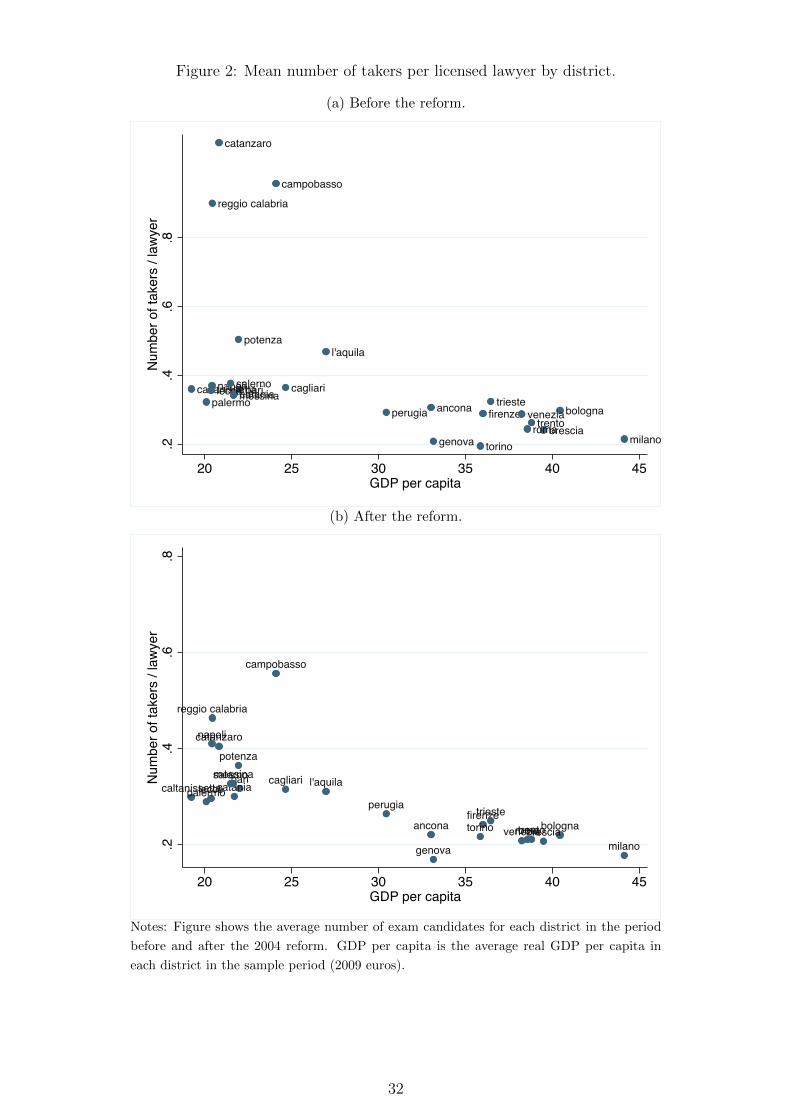
Figure 2: Mean number of takers per licensed lawyer by district.

(a) Before the reform.

anconabari

bologna

brescia

cagliaricaltanissetta

campobasso

catania

catanzaro

firenze

genova

l'aquila

leccemessina

milano

napolipalermo

perugia

potenza

reggio calabria

roma

salerno

torino

trento

triestevenezia

.2.4

.6.8

Num

ber o

f tak

ers

/ law

yer

20 25 30 35 40 45GDP per capita

(b) After the reform.

ancona

bari

bolognabrescia

cagliaricaltanissetta

campobasso

catania

catanzaro

firenze

genova

l'aquilaleccemessina

milano

napoli

palermoperugia

potenza

reggio calabria

roma

salerno

torino trentotrieste

venezia

.2.4

.6.8

Num

ber o

f tak

ers

/ law

yer

20 25 30 35 40 45GDP per capita

Notes: Figure shows the average number of exam candidates for each district in the period

before and after the 2004 reform. GDP per capita is the average real GDP per capita in

each district in the sample period (2009 euros).

32

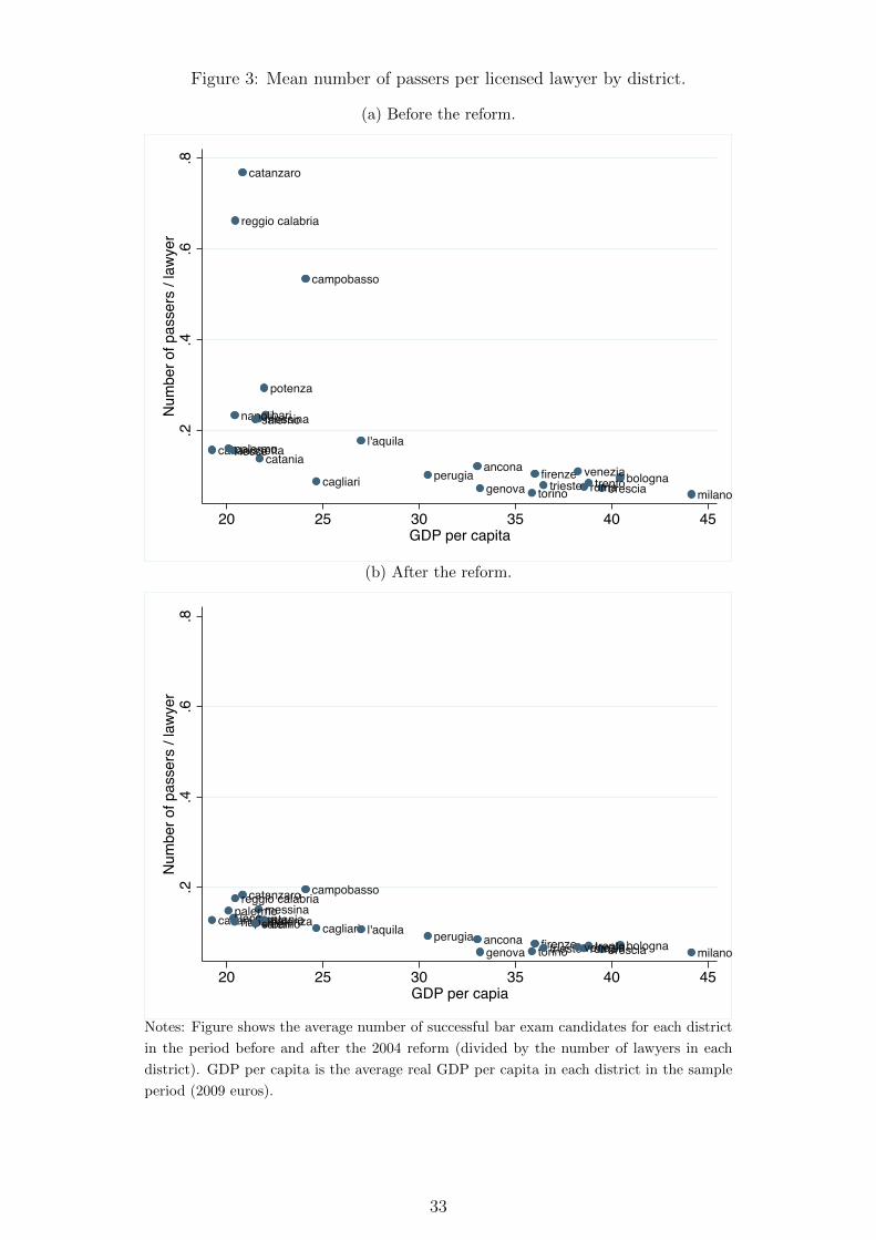
Figure 3: Mean number of passers per licensed lawyer by district.

(a) Before the reform.

ancona

bari

bolognabresciacagliari

caltanissetta

campobasso

catania

catanzaro

firenzegenova

l'aquilalecce

messina

milano

napoli

palermo

perugia

potenza

reggio calabria

roma

salerno

torinotrentotrieste

venezia

.2.4

.6.8

Num

ber o

f pas

sers

/ la

wye

r

20 25 30 35 40 45GDP per capita

(b) After the reform.

anconabari

bolognabrescia

cagliaricaltanissetta

campobasso

catania

catanzaro

firenzegenova

l'aquilalecce

messina

milano

napolipalermo

perugiapotenza

reggio calabria

roma

salerno

torino trentotrieste venezia

.2.4

.6.8

Num

ber o

f pas

sers

/ la

wye

r

20 25 30 35 40 45GDP per capia

Notes: Figure shows the average number of successful bar exam candidates for each district

in the period before and after the 2004 reform (divided by the number of lawyers in each

district). GDP per capita is the average real GDP per capita in each district in the sample

period (2009 euros).

33

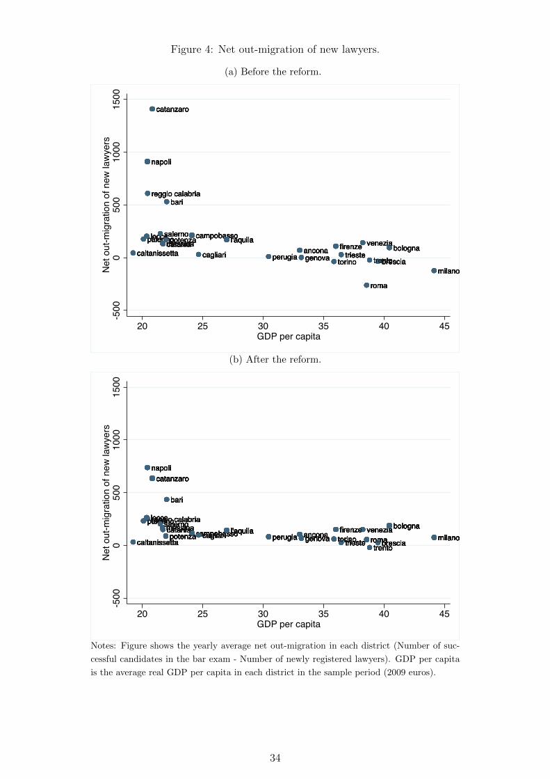
Figure 4: Net out-migration of new lawyers.

(a) Before the reform.

veneziacagliari trieste

l'aquilalecce

roma

bologna

catanzaro

salernocatania firenze

bari

trento

palermopotenzaancona

brescia

messina

napoli

genova torinomilano

caltanissetta

campobasso

perugia

reggio calabria

napoli

firenze

catanzaro

campobassomessina

ancona bolognapalermo

cagliaritorinogenova

reggio calabria

lecce potenza veneziacaltanissetta trieste

milanotrentoperugia

roma

bari

catania

brescia

salernol'aquilalecce

genovacaltanissetta ancona

catanzaro

campobassomessina

torinocagliari

palermobologna

perugia trento

firenze

roma

napoli

l'aquila

milano

salerno

bari

trieste

reggio calabria

veneziapotenza

brescia

catania venezia

roma

catanzaro

genovacaltanissetta

milanotorino

napoli

bologna

salernol'aquilapotenzapalermomessina

brescia

catania

reggio calabria

ancona

campobasso

bari

cagliari perugia

leccefirenze

trentotrieste

napoli

caltanissettabrescia

potenza

trentobologna

trieste

roma

reggio calabria

milano

ancona

catanzaro

campobassosalernol'aquila

perugiacagliarimessina veneziacatania

genova

bari

torino

palermoleccefirenze bologna

palermo campobasso

genova

l'aquilacatania venezia

reggio calabria

napoli

catanzaro

lecce

cagliaribrescia

milano

potenzacaltanissetta perugia

messinatrieste

salerno

bari

trentotorino

roma

ancona firenze

-500

050

010

0015

00N

et o

ut-m

igra

tion

of n

ew la

wye

rs

20 25 30 35 40 45GDP per capita

(b) After the reform.

napoli

perugia

bari

catanzaro

genova brescia

leccemessina

trieste

bolognapotenza

catania venezial'aquilaroma

reggio calabria

ancona firenzepalermo

torinotrento

caltanissetta milano

salernocagliaricampobassocampobasso

bari

trieste

catanzaro

milanoanconacataniasalernopalermo

cagliari

leccebologna

bresciafirenze

napoli

roma

reggio calabriaveneziamessina

trento

l'aquilapotenza genova torinoperugiacaltanissetta

salernol'aquila

bari

catania veneziacagliari ancona

bologna

catanzaro

reggio calabria

campobassopotenza torinocaltanissetta roma

napoli

firenze

trentoperugia

bresciagenova milanotrieste

leccepalermomessina l'aquila

reggio calabria

triesteveneziacampobasso ancona

catanzaro

romacaltanissettacatania

salerno bolognagenovapotenza cagliari

lecce

torinotrento

perugia

napoli

firenzemilano

brescia

palermo

bari

messina l'aquilatorinocagliari

bolognamessinacampobasso

catanzaro

romacatania

milano

salernolecce

trentobrescia

bari

perugia

reggio calabriafirenze

caltanissetta

palermo

ancona

napoli

genovapotenzatrieste

veneziasalerno

l'aquilapalermo

cagliari milanotorino

lecce

genova

bari

campobassotrieste

perugiabolognafirenze

caltanissettaancona

trento

napoli

messina

bresciavenezia

potenza

catanzaro

cataniaroma

reggio calabriacatania

palermo

bresciapotenza

trieste

napoli

reggio calabria

catanzaro

roma

bari

milanoperugia ancona torinoveneziacampobasso

salernofirenzel'aquila bologna

caltanissettacagliari

messina

trento

lecce

genovacampobasso

lecce

bari

messina bolognasalerno

brescia

catanzaro

ancona torinovenezia

cagliari romatrento

perugiapotenza genovacaltanissetta

napoli

reggio calabria

milanofirenzel'aquila

triestecatania

palermo

genovacampobasso

reggio calabrialecce

potenzaveneziacatania

palermomessina

cagliaribologna

anconatrentotriestetorinocaltanissetta brescia

firenzeroma

l'aquila

bari

salernoperugia

catanzaro

milano

napoli

-500

050

010

0015

00N

et o

ut-m

igra

tion

of n

ew la

wye

rs

20 25 30 35 40 45GDP per capita

Notes: Figure shows the yearly average net out-migration in each district (Number of suc-

cessful candidates in the bar exam - Number of newly registered lawyers). GDP per capita

is the average real GDP per capita in each district in the sample period (2009 euros).

34

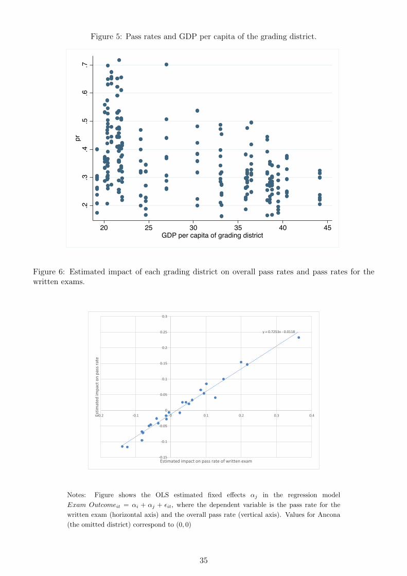
Figure 5: Pass rates and GDP per capita of the grading district.

.2.3

.4.5

.6.7

pr

20 25 30 35 40 45GDP per capita of grading district

Figure 6: Estimated impact of each grading district on overall pass rates and pass rates for thewritten exams.

y = 0.7253x - 0.0118

-0.15

-0.1

-0.05

0

0.05

0.1

0.15

0.2

0.25

0.3

-0.2 -0.1 0 0.1 0.2 0.3 0.4Esti

mat

ed im

pac

t o

n p

ass

rate

Estimated impact on pass rate of written exam

Notes: Figure shows the OLS estimated fixed effects αj in the regression model

Exam Outcomeit = αi + αj + εit, where the dependent variable is the pass rate for the

written exam (horizontal axis) and the overall pass rate (vertical axis). Values for Ancona

(the omitted district) correspond to (0, 0)

35

Figure 7: Estimated impact of each grading district on pass rates for the oral and written exams.

y = -0.2004x - 0.0293

-0.14

-0.12

-0.1

-0.08

-0.06

-0.04

-0.02

0

0.02

0.04

-0.2 -0.1 0 0.1 0.2 0.3 0.4

Esti

mat

ed im

pac

t o

n p

ass

rate

of

ora

l exa

m

Estimated impact on pass rate of written exam

Notes: Figure shows the OLS estimated fixed effects αj in the regression model

Exam Outcomeit = αi + αj + εit, where the dependent variable is the pass rate for the

written exam (horizontal axis) and the pass rate for the oral exam (vertical axis). Values for

Ancona (the omitted district) correspond to (0, 0)

Figure 8: Empirical model of the admission process.

qr

qw

Area A: Fail

written

Area C: Pass

written and oral

Area B: Pass written,

fail oral

w

r

Notes: Figure shows exam outcomes as a function of grading thresholds for a population of

exam candidates with a performance distribution described by (4).

36

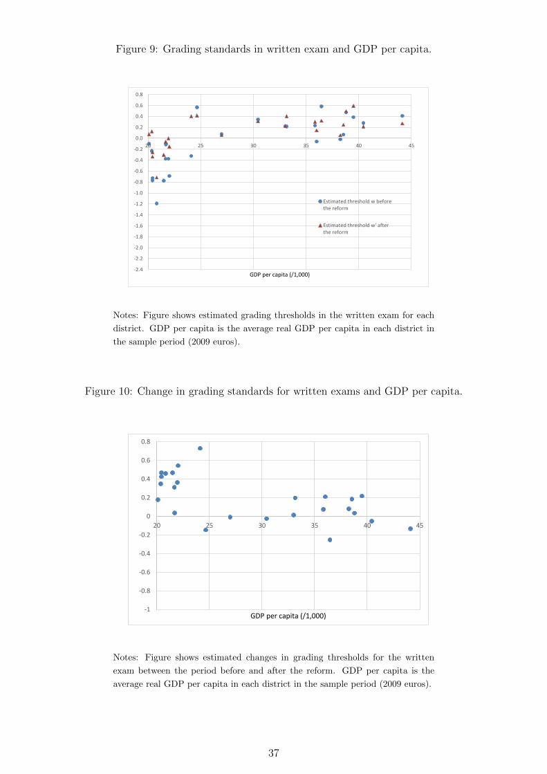
Figure 9: Grading standards in written exam and GDP per capita.

-2.4

-2.2

-2.0

-1.8

-1.6

-1.4

-1.2

-1.0

-0.8

-0.6

-0.4

-0.2

0.0

0.2

0.4

0.6

0.8

20 25 30 35 40 45

GDP per capita (/1,000)

Estimated threshold w beforethe reform

Estimated threshold w' afterthe reform

Notes: Figure shows estimated grading thresholds in the written exam for each

district. GDP per capita is the average real GDP per capita in each district in

the sample period (2009 euros).

Figure 10: Change in grading standards for written exams and GDP per capita.

-1

-0.8

-0.6

-0.4

-0.2

0

0.2

0.4

0.6

0.8

20 25 30 35 40 45

GDP per capita (/1,000)

Notes: Figure shows estimated changes in grading thresholds for the written

exam between the period before and after the reform. GDP per capita is the

average real GDP per capita in each district in the sample period (2009 euros).

37

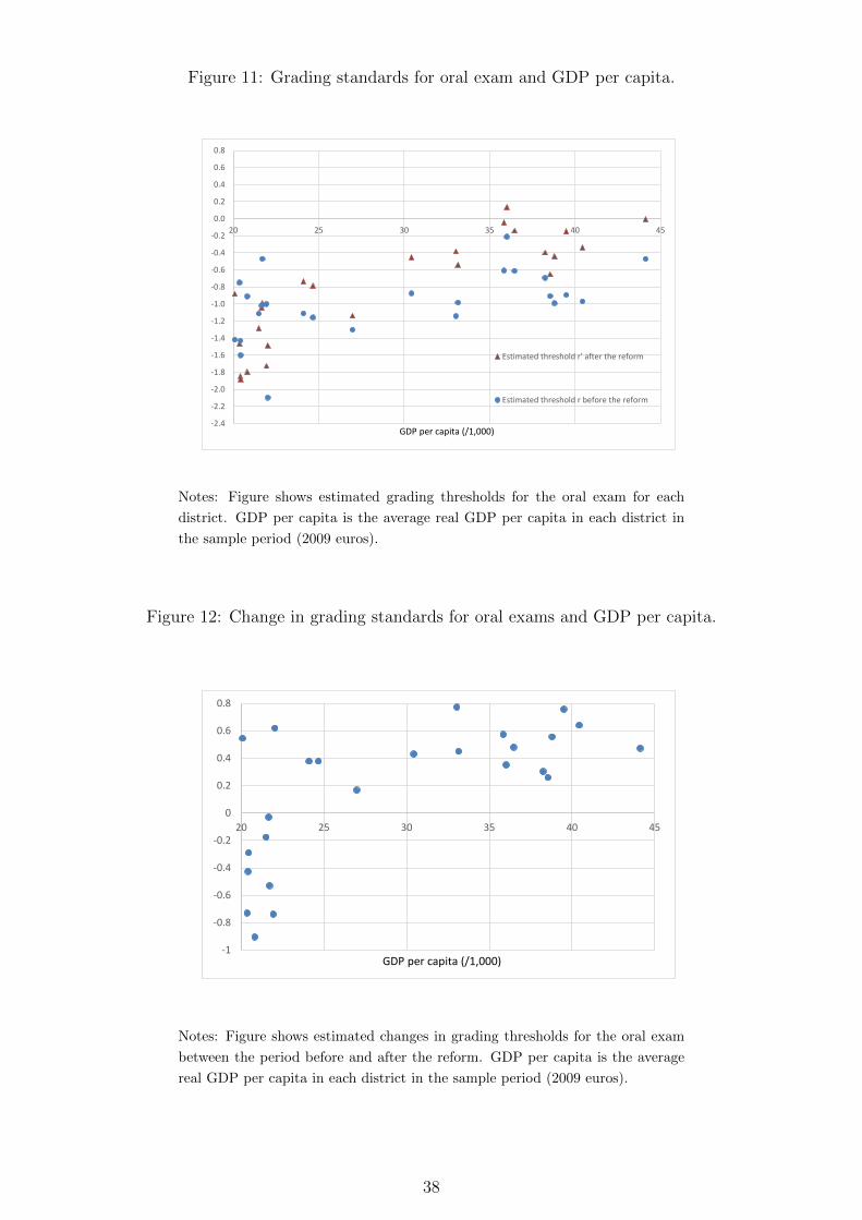
Figure 11: Grading standards for oral exam and GDP per capita.

-2.4

-2.2

-2.0

-1.8

-1.6

-1.4

-1.2

-1.0

-0.8

-0.6

-0.4

-0.2

0.0

0.2

0.4

0.6

0.8

20 25 30 35 40 45

GDP per capita (/1,000)

Estimated threshold r' after the reform

Estimated threshold r before the reform

Notes: Figure shows estimated grading thresholds for the oral exam for each

district. GDP per capita is the average real GDP per capita in each district in

the sample period (2009 euros).

Figure 12: Change in grading standards for oral exams and GDP per capita.

-1

-0.8

-0.6

-0.4

-0.2

0

0.2

0.4

0.6

0.8

20 25 30 35 40 45

GDP per capita (/1,000)

Notes: Figure shows estimated changes in grading thresholds for the oral exam

between the period before and after the reform. GDP per capita is the average

real GDP per capita in each district in the sample period (2009 euros).

38

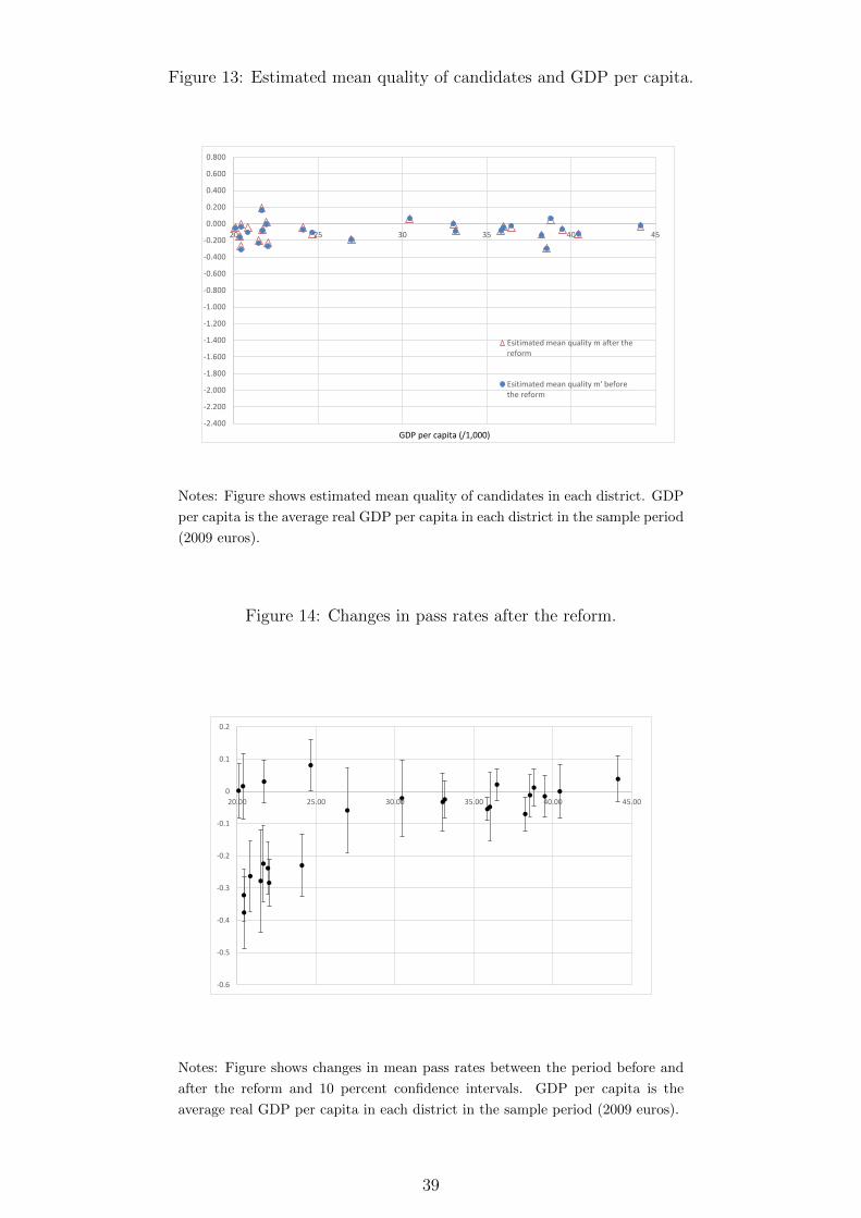
Figure 13: Estimated mean quality of candidates and GDP per capita.

-2.400

-2.200

-2.000

-1.800

-1.600

-1.400

-1.200

-1.000

-0.800

-0.600

-0.400

-0.200

0.000

0.200

0.400

0.600

0.800

20 25 30 35 40 45

GDP per capita (/1,000)

Esitimated mean quality m after thereform

Esitimated mean quality m' beforethe reform

Notes: Figure shows estimated mean quality of candidates in each district. GDP

per capita is the average real GDP per capita in each district in the sample period

(2009 euros).

Figure 14: Changes in pass rates after the reform.

-0.6

-0.5

-0.4

-0.3

-0.2

-0.1

0

0.1

0.2

20.00 25.00 30.00 35.00 40.00 45.00

Notes: Figure shows changes in mean pass rates between the period before and

after the reform and 10 percent confidence intervals. GDP per capita is the

average real GDP per capita in each district in the sample period (2009 euros).

39

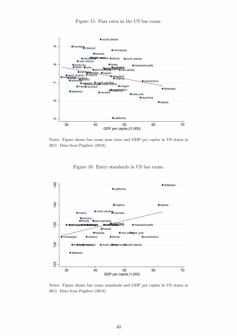
Figure 15: Pass rates in the US bar exam.

alabama

alaska

arizonaarkansas

california

colorado

connecticut

delaware

florida

georgia hawaii

idaho

illinois

indiana

iowakansas

kentucky

louisianamaine

maryland

massachusetts

michigan

minnesota

mississippi

missourimontana

nebraska

nevada

new hampshirenew jersey

new mexico

new york

north carolina

north dakota

ohio

oklahoma

oregon

pennsylvania

rhode island

south carolina

south dakota

tennessee

texas

utah

vermont

virginia

washington

west virginia

wisconsin

wyoming

.5.6

.7.8

.9

30 40 50 60 70GDP per capita (/1,000)

Notes: Figure shows bar exam pass rates and GDP per capita in US states in

2011. Data from Pagliero (2013).

Figure 16: Entry standards in US bar exam.

alabama

alaska

arizona

arkansas

california

colorado

connecticut

delaware

floridageorgia

hawaii

illinoisindianakansas

maine

maryland massachusetts

minnesota

mississippi

missourimontana

nebraskanew hampshire

new jersey

new mexico

new york

north carolina

north dakota

ohiooklahomapennsylvania

south dakota

texasutah

virginia

west virginia

125

130

135

140

145

30 40 50 60 70GDP per capita (1,000)

Notes: Figure shows bar exam standards and GDP per capita in US states in

2011. Data from Pagliero (2013).

40

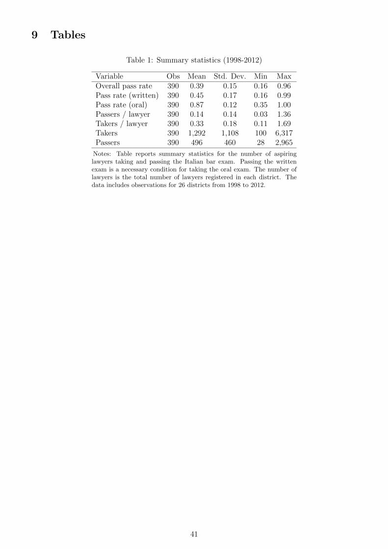
9 Tables

Table 1: Summary statistics (1998-2012)

Variable Obs Mean Std. Dev. Min MaxOverall pass rate 390 0.39 0.15 0.16 0.96Pass rate (written) 390 0.45 0.17 0.16 0.99Pass rate (oral) 390 0.87 0.12 0.35 1.00Passers / lawyer 390 0.14 0.14 0.03 1.36Takers / lawyer 390 0.33 0.18 0.11 1.69Takers 390 1,292 1,108 100 6,317Passers 390 496 460 28 2,965

Notes: Table reports summary statistics for the number of aspiringlawyers taking and passing the Italian bar exam. Passing the writtenexam is a necessary condition for taking the oral exam. The number oflawyers is the total number of lawyers registered in each district. Thedata includes observations for 26 districts from 1998 to 2012.

41

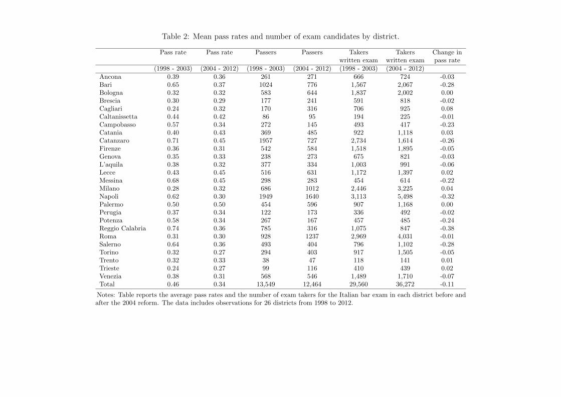
Table 2: Mean pass rates and number of exam candidates by district.

Pass rate Pass rate Passers Passers Takers Takers Change inwritten exam written exam pass rate

(1998 - 2003) (2004 - 2012) (1998 - 2003) (2004 - 2012) (1998 - 2003) (2004 - 2012)Ancona 0.39 0.36 261 271 666 724 -0.03Bari 0.65 0.37 1024 776 1,567 2,067 -0.28Bologna 0.32 0.32 583 644 1,837 2,002 0.00Brescia 0.30 0.29 177 241 591 818 -0.02Cagliari 0.24 0.32 170 316 706 925 0.08Caltanissetta 0.44 0.42 86 95 194 225 -0.01Campobasso 0.57 0.34 272 145 493 417 -0.23Catania 0.40 0.43 369 485 922 1,118 0.03Catanzaro 0.71 0.45 1957 727 2,734 1,614 -0.26Firenze 0.36 0.31 542 584 1,518 1,895 -0.05Genova 0.35 0.33 238 273 675 821 -0.03L’aquila 0.38 0.32 377 334 1,003 991 -0.06Lecce 0.43 0.45 516 631 1,172 1,397 0.02Messina 0.68 0.45 298 283 454 614 -0.22Milano 0.28 0.32 686 1012 2,446 3,225 0.04Napoli 0.62 0.30 1949 1640 3,113 5,498 -0.32Palermo 0.50 0.50 454 596 907 1,168 0.00Perugia 0.37 0.34 122 173 336 492 -0.02Potenza 0.58 0.34 267 167 457 485 -0.24Reggio Calabria 0.74 0.36 785 316 1,075 847 -0.38Roma 0.31 0.30 928 1237 2,969 4,031 -0.01Salerno 0.64 0.36 493 404 796 1,102 -0.28Torino 0.32 0.27 294 403 917 1,505 -0.05Trento 0.32 0.33 38 47 118 141 0.01Trieste 0.24 0.27 99 116 410 439 0.02Venezia 0.38 0.31 568 546 1,489 1,710 -0.07Total 0.46 0.34 13,549 12,464 29,560 36,272 -0.11

Notes: Table reports the average pass rates and the number of exam takers for the Italian bar exam in each district before andafter the 2004 reform. The data includes observations for 26 districts from 1998 to 2012.

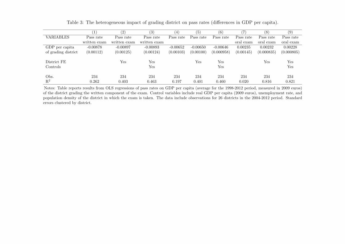
Table 3: The heterogeneous impact of grading district on pass rates (differences in GDP per capita).

(1) (2) (3) (4) (5) (6) (7) (8) (9)VARIABLES Pass rate Pass rate Pass rate Pass rate Pass rate Pass rate Pass rate Pass rate Pass rate

written exam written exam written exam oral exam oral exam oral examGDP per capita -0.00878 -0.00897 -0.00893 -0.00652 -0.00650 -0.00646 0.00235 0.00232 0.00228of grading district (0.00112) (0.00125) (0.00124) (0.00103) (0.00100) (0.000958) (0.00145) (0.000835) (0.000805)

District FE Yes Yes Yes Yes Yes YesControls Yes Yes Yes

Obs. 234 234 234 234 234 234 234 234 234R2 0.262 0.403 0.463 0.197 0.401 0.460 0.020 0.816 0.821

Notes: Table reports results from OLS regressions of pass rates on GDP per capita (average for the 1998-2012 period, measured in 2009 euros)of the district grading the written component of the exam. Control variables include real GDP per capita (2009 euros), unemployment rate, andpopulation density of the district in which the exam is taken. The data include observations for 26 districts in the 2004-2012 period. Standarderrors clustered by district.

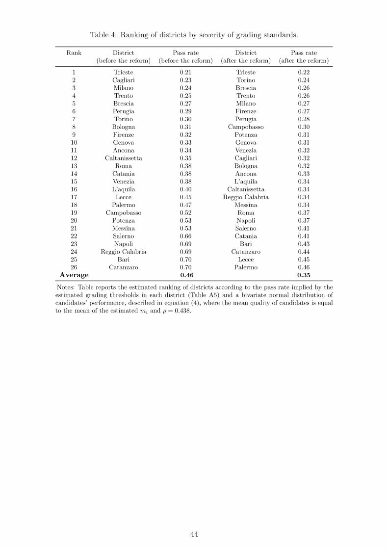
Table 4: Ranking of districts by severity of grading standards.

Rank District Pass rate District Pass rate(before the reform) (before the reform) (after the reform) (after the reform)

1 Trieste 0.21 Trieste 0.222 Cagliari 0.23 Torino 0.243 Milano 0.24 Brescia 0.264 Trento 0.25 Trento 0.265 Brescia 0.27 Milano 0.276 Perugia 0.29 Firenze 0.277 Torino 0.30 Perugia 0.288 Bologna 0.31 Campobasso 0.309 Firenze 0.32 Potenza 0.3110 Genova 0.33 Genova 0.3111 Ancona 0.34 Venezia 0.3212 Caltanissetta 0.35 Cagliari 0.3213 Roma 0.38 Bologna 0.3214 Catania 0.38 Ancona 0.3315 Venezia 0.38 L’aquila 0.3416 L’aquila 0.40 Caltanissetta 0.3417 Lecce 0.45 Reggio Calabria 0.3418 Palermo 0.47 Messina 0.3419 Campobasso 0.52 Roma 0.3720 Potenza 0.53 Napoli 0.3721 Messina 0.53 Salerno 0.4122 Salerno 0.66 Catania 0.4123 Napoli 0.69 Bari 0.4324 Reggio Calabria 0.69 Catanzaro 0.4425 Bari 0.70 Lecce 0.4526 Catanzaro 0.70 Palermo 0.46

Average 0.46 0.35

Notes: Table reports the estimated ranking of districts according to the pass rate implied by theestimated grading thresholds in each district (Table A5) and a bivariate normal distribution ofcandidates’ performance, described in equation (4), where the mean quality of candidates is equalto the mean of the estimated mi and ρ = 0.438.

44

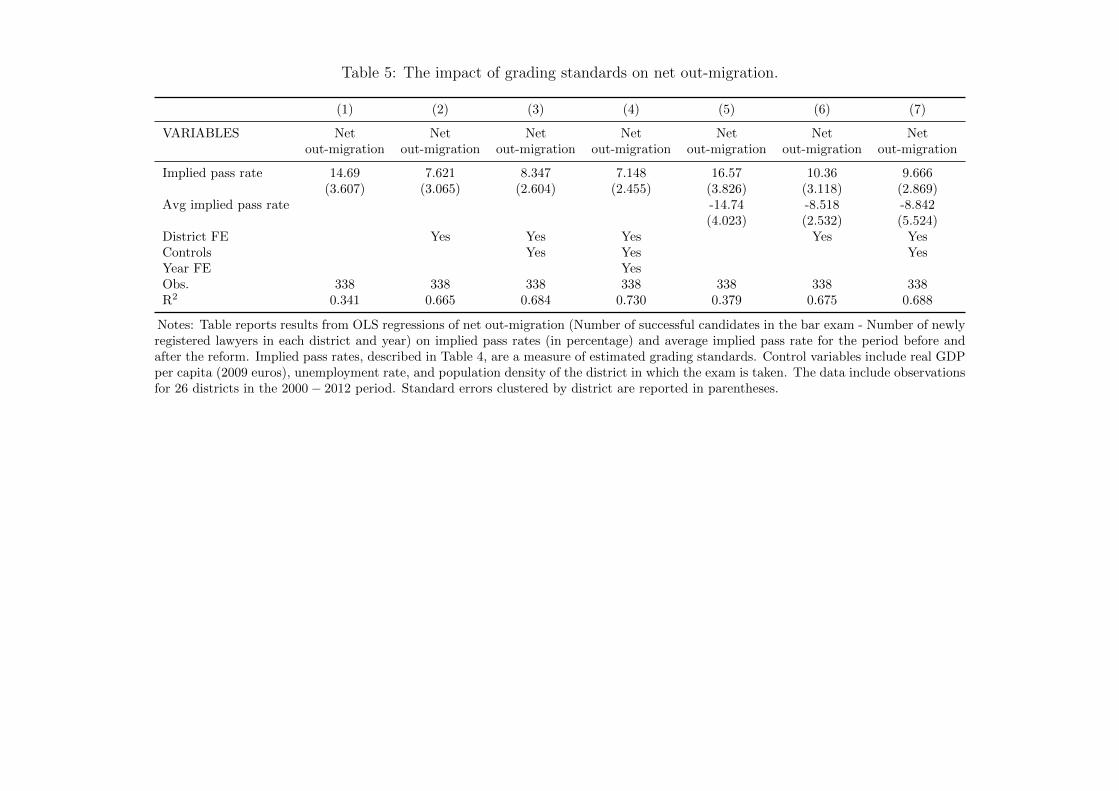
Table 5: The impact of grading standards on net out-migration.

(1) (2) (3) (4) (5) (6) (7)

VARIABLES Net Net Net Net Net Net Netout-migration out-migration out-migration out-migration out-migration out-migration out-migration

Implied pass rate 14.69 7.621 8.347 7.148 16.57 10.36 9.666(3.607) (3.065) (2.604) (2.455) (3.826) (3.118) (2.869)

Avg implied pass rate -14.74 -8.518 -8.842(4.023) (2.532) (5.524)

District FE Yes Yes Yes Yes YesControls Yes Yes YesYear FE YesObs. 338 338 338 338 338 338 338R2 0.341 0.665 0.684 0.730 0.379 0.675 0.688

Notes: Table reports results from OLS regressions of net out-migration (Number of successful candidates in the bar exam - Number of newlyregistered lawyers in each district and year) on implied pass rates (in percentage) and average implied pass rate for the period before andafter the reform. Implied pass rates, described in Table 4, are a measure of estimated grading standards. Control variables include real GDPper capita (2009 euros), unemployment rate, and population density of the district in which the exam is taken. The data include observationsfor 26 districts in the 2000− 2012 period. Standard errors clustered by district are reported in parentheses.

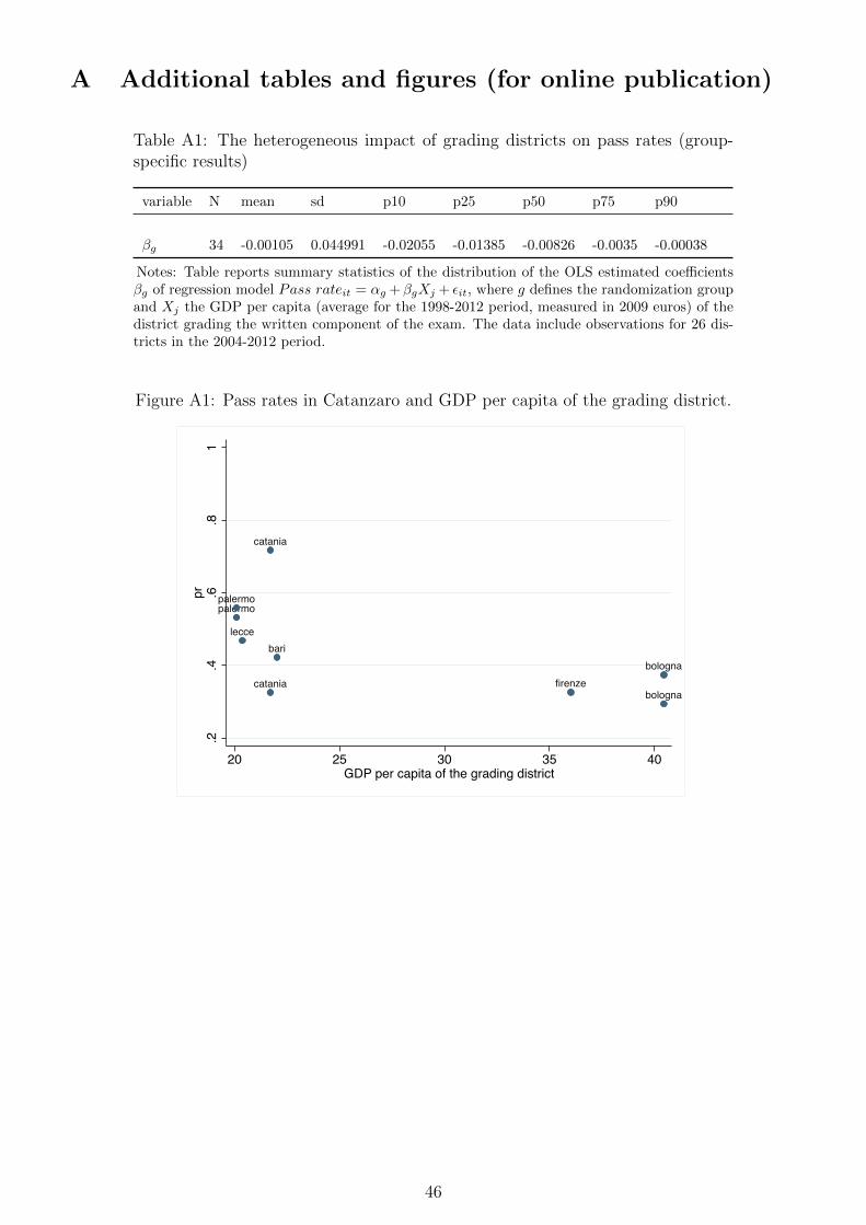
A Additional tables and figures (for online publication)

Table A1: The heterogeneous impact of grading districts on pass rates (group-specific results)

variable N mean sd p10 p25 p50 p75 p90

βg 34 -0.00105 0.044991 -0.02055 -0.01385 -0.00826 -0.0035 -0.00038

Notes: Table reports summary statistics of the distribution of the OLS estimated coefficientsβg of regression model Pass rateit = αg + βgXj + εit, where g defines the randomization groupand Xj the GDP per capita (average for the 1998-2012 period, measured in 2009 euros) of thedistrict grading the written component of the exam. The data include observations for 26 dis-tricts in the 2004-2012 period.

Figure A1: Pass rates in Catanzaro and GDP per capita of the grading district.

firenze

palermo

catania

lecce

palermo

cataniabologna

bolognabari

.2.4

.6.8

1pr

20 25 30 35 40GDP per capita of the grading district

46

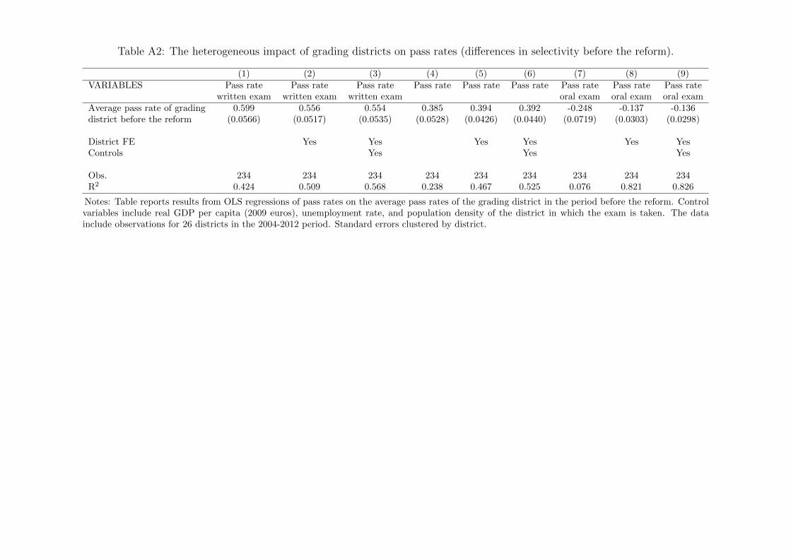
Table A2: The heterogeneous impact of grading districts on pass rates (differences in selectivity before the reform).

(1) (2) (3) (4) (5) (6) (7) (8) (9)VARIABLES Pass rate Pass rate Pass rate Pass rate Pass rate Pass rate Pass rate Pass rate Pass rate

written exam written exam written exam oral exam oral exam oral examAverage pass rate of grading 0.599 0.556 0.554 0.385 0.394 0.392 -0.248 -0.137 -0.136district before the reform (0.0566) (0.0517) (0.0535) (0.0528) (0.0426) (0.0440) (0.0719) (0.0303) (0.0298)

District FE Yes Yes Yes Yes Yes YesControls Yes Yes Yes

Obs. 234 234 234 234 234 234 234 234 234R2 0.424 0.509 0.568 0.238 0.467 0.525 0.076 0.821 0.826

Notes: Table reports results from OLS regressions of pass rates on the average pass rates of the grading district in the period before the reform. Controlvariables include real GDP per capita (2009 euros), unemployment rate, and population density of the district in which the exam is taken. The datainclude observations for 26 districts in the 2004-2012 period. Standard errors clustered by district.

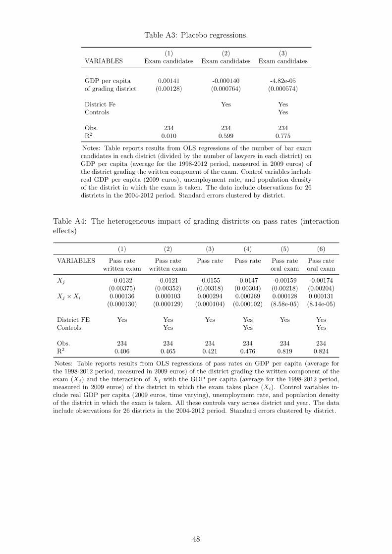
Table A3: Placebo regressions.

(1) (2) (3)VARIABLES Exam candidates Exam candidates Exam candidates

GDP per capita 0.00141 -0.000140 -4.82e-05of grading district (0.00128) (0.000764) (0.000574)

District Fe Yes YesControls Yes

Obs. 234 234 234R2 0.010 0.599 0.775

Notes: Table reports results from OLS regressions of the number of bar examcandidates in each district (divided by the number of lawyers in each district) onGDP per capita (average for the 1998-2012 period, measured in 2009 euros) ofthe district grading the written component of the exam. Control variables includereal GDP per capita (2009 euros), unemployment rate, and population densityof the district in which the exam is taken. The data include observations for 26districts in the 2004-2012 period. Standard errors clustered by district.

Table A4: The heterogeneous impact of grading districts on pass rates (interactioneffects)

(1) (2) (3) (4) (5) (6)

VARIABLES Pass rate Pass rate Pass rate Pass rate Pass rate Pass ratewritten exam written exam oral exam oral exam

Xj -0.0132 -0.0121 -0.0155 -0.0147 -0.00159 -0.00174(0.00375) (0.00352) (0.00318) (0.00304) (0.00218) (0.00204)

Xj ×Xi 0.000136 0.000103 0.000294 0.000269 0.000128 0.000131(0.000130) (0.000129) (0.000104) (0.000102) (8.58e-05) (8.14e-05)

District FE Yes Yes Yes Yes Yes YesControls Yes Yes Yes

Obs. 234 234 234 234 234 234R2 0.406 0.465 0.421 0.476 0.819 0.824

Notes: Table reports results from OLS regressions of pass rates on GDP per capita (average forthe 1998-2012 period, measured in 2009 euros) of the district grading the written component of theexam (Xj) and the interaction of Xj with the GDP per capita (average for the 1998-2012 period,measured in 2009 euros) of the district in which the exam takes place (Xi). Control variables in-clude real GDP per capita (2009 euros, time varying), unemployment rate, and population densityof the district in which the exam is taken. All these controls vary across district and year. The datainclude observations for 26 districts in the 2004-2012 period. Standard errors clustered by district.

48

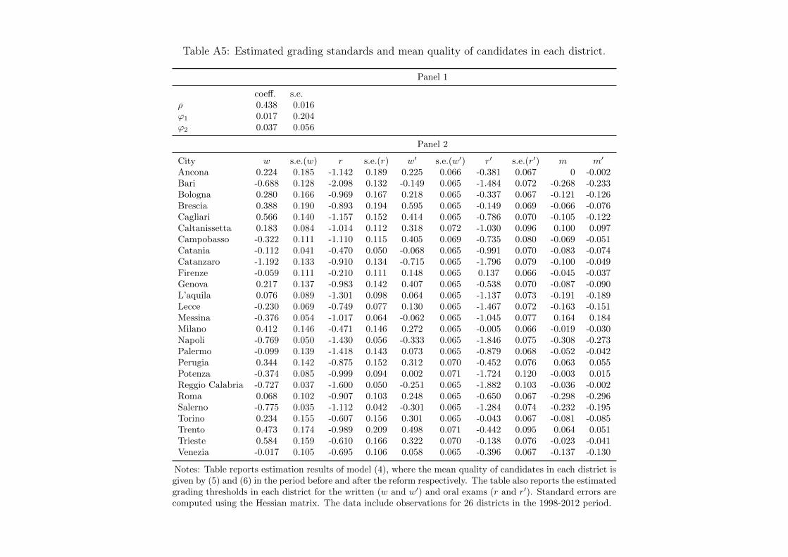
Table A5: Estimated grading standards and mean quality of candidates in each district.

Panel 1

coeff. s.e.ρ 0.438 0.016ϕ1 0.017 0.204ϕ2 0.037 0.056

Panel 2

City w s.e.(w) r s.e.(r) w′ s.e.(w′) r′ s.e.(r′) m m′

Ancona 0.224 0.185 -1.142 0.189 0.225 0.066 -0.381 0.067 0 -0.002Bari -0.688 0.128 -2.098 0.132 -0.149 0.065 -1.484 0.072 -0.268 -0.233Bologna 0.280 0.166 -0.969 0.167 0.218 0.065 -0.337 0.067 -0.121 -0.126Brescia 0.388 0.190 -0.893 0.194 0.595 0.065 -0.149 0.069 -0.066 -0.076Cagliari 0.566 0.140 -1.157 0.152 0.414 0.065 -0.786 0.070 -0.105 -0.122Caltanissetta 0.183 0.084 -1.014 0.112 0.318 0.072 -1.030 0.096 0.100 0.097Campobasso -0.322 0.111 -1.110 0.115 0.405 0.069 -0.735 0.080 -0.069 -0.051Catania -0.112 0.041 -0.470 0.050 -0.068 0.065 -0.991 0.070 -0.083 -0.074Catanzaro -1.192 0.133 -0.910 0.134 -0.715 0.065 -1.796 0.079 -0.100 -0.049Firenze -0.059 0.111 -0.210 0.111 0.148 0.065 0.137 0.066 -0.045 -0.037Genova 0.217 0.137 -0.983 0.142 0.407 0.065 -0.538 0.070 -0.087 -0.090L’aquila 0.076 0.089 -1.301 0.098 0.064 0.065 -1.137 0.073 -0.191 -0.189Lecce -0.230 0.069 -0.749 0.077 0.130 0.065 -1.467 0.072 -0.163 -0.151Messina -0.376 0.054 -1.017 0.064 -0.062 0.065 -1.045 0.077 0.164 0.184Milano 0.412 0.146 -0.471 0.146 0.272 0.065 -0.005 0.066 -0.019 -0.030Napoli -0.769 0.050 -1.430 0.056 -0.333 0.065 -1.846 0.075 -0.308 -0.273Palermo -0.099 0.139 -1.418 0.143 0.073 0.065 -0.879 0.068 -0.052 -0.042Perugia 0.344 0.142 -0.875 0.152 0.312 0.070 -0.452 0.076 0.063 0.055Potenza -0.374 0.085 -0.999 0.094 0.002 0.071 -1.724 0.120 -0.003 0.015Reggio Calabria -0.727 0.037 -1.600 0.050 -0.251 0.065 -1.882 0.103 -0.036 -0.002Roma 0.068 0.102 -0.907 0.103 0.248 0.065 -0.650 0.067 -0.298 -0.296Salerno -0.775 0.035 -1.112 0.042 -0.301 0.065 -1.284 0.074 -0.232 -0.195Torino 0.234 0.155 -0.607 0.156 0.301 0.065 -0.043 0.067 -0.081 -0.085Trento 0.473 0.174 -0.989 0.209 0.498 0.071 -0.442 0.095 0.064 0.051Trieste 0.584 0.159 -0.610 0.166 0.322 0.070 -0.138 0.076 -0.023 -0.041Venezia -0.017 0.105 -0.695 0.106 0.058 0.065 -0.396 0.067 -0.137 -0.130

Notes: Table reports estimation results of model (4), where the mean quality of candidates in each district isgiven by (5) and (6) in the period before and after the reform respectively. The table also reports the estimatedgrading thresholds in each district for the written (w and w′) and oral exams (r and r′). Standard errors arecomputed using the Hessian matrix. The data include observations for 26 districts in the 1998-2012 period.

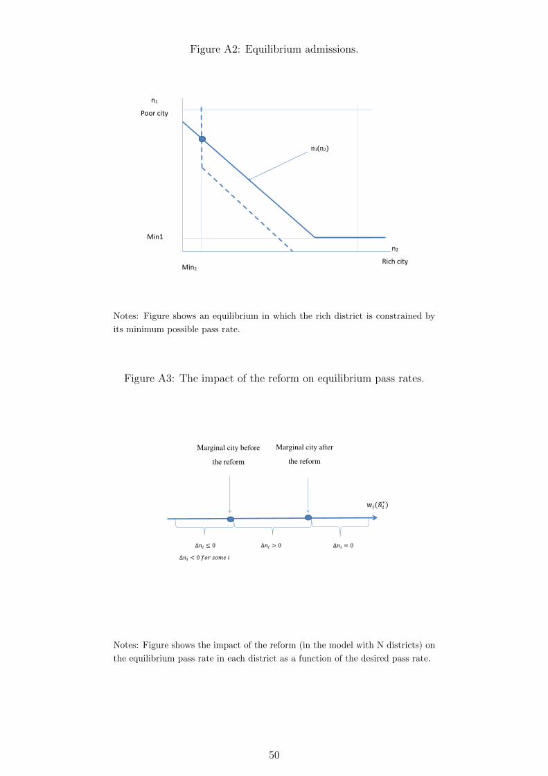
Figure A2: Equilibrium admissions.

n1

Poor city

n2

Rich city

n1(n2)

Min1

Min2

Notes: Figure shows an equilibrium in which the rich district is constrained by

its minimum possible pass rate.

Figure A3: The impact of the reform on equilibrium pass rates.

��(���∗)

Marginal city before

the reform

∆�� ≤ 0

∆�� < 0 �������

∆�� > 0 ∆�� = 0

Marginal city after

the reform

Notes: Figure shows the impact of the reform (in the model with N districts) on

the equilibrium pass rate in each district as a function of the desired pass rate.

50

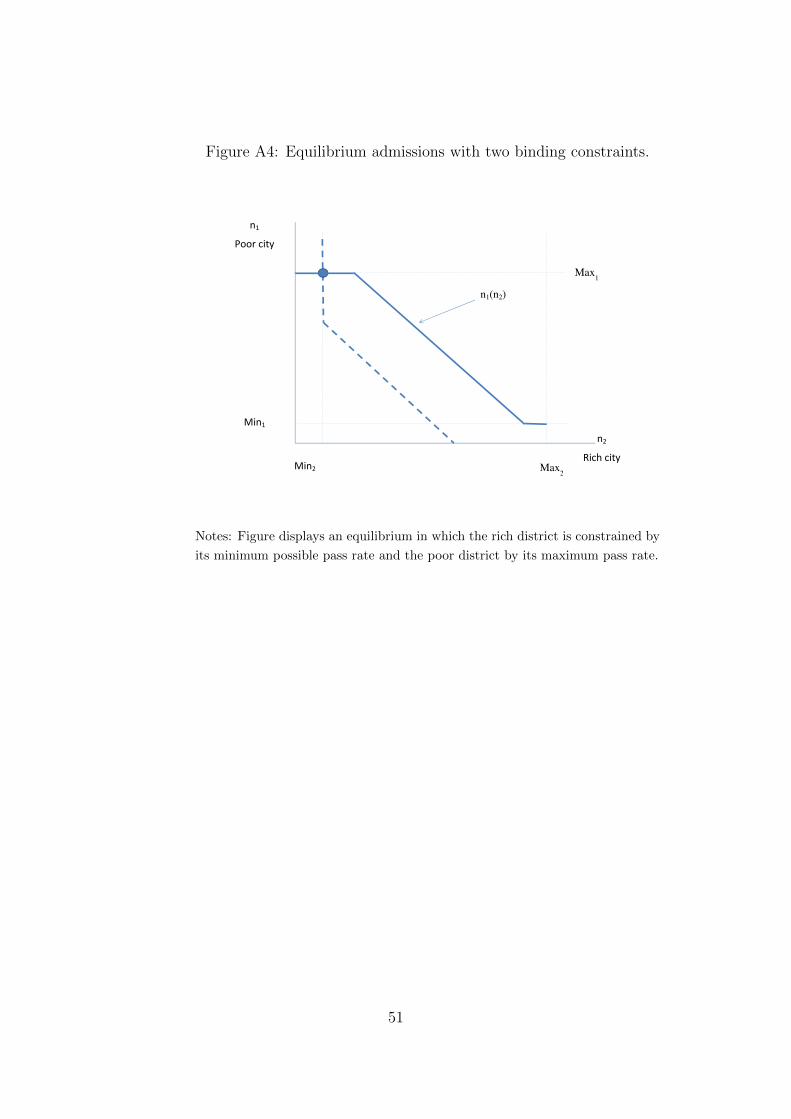
Figure A4: Equilibrium admissions with two binding constraints.

n1

Poor city

n2

Rich city

n1(n2)

Min1

Min2

Max1

Max2

Notes: Figure displays an equilibrium in which the rich district is constrained by

its minimum possible pass rate and the poor district by its maximum pass rate.

51

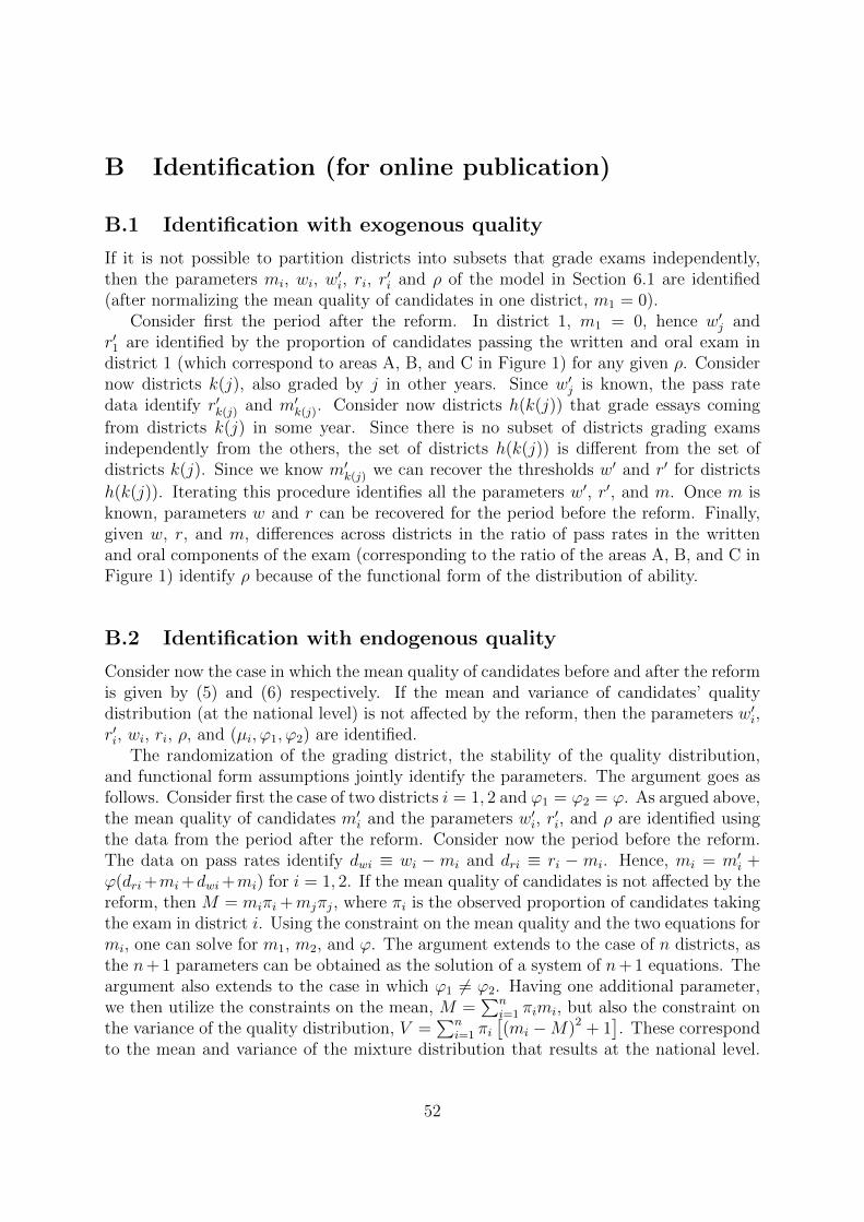
B Identification (for online publication)

B.1 Identification with exogenous quality

If it is not possible to partition districts into subsets that grade exams independently,then the parameters mi, wi, w

′i, ri, r

′i and ρ of the model in Section 6.1 are identified

(after normalizing the mean quality of candidates in one district, m1 = 0).Consider first the period after the reform. In district 1, m1 = 0, hence w′j and

r′1 are identified by the proportion of candidates passing the written and oral exam indistrict 1 (which correspond to areas A, B, and C in Figure 1) for any given ρ. Considernow districts k(j), also graded by j in other years. Since w′j is known, the pass ratedata identify r′k(j) and m′k(j). Consider now districts h(k(j)) that grade essays coming

from districts k(j) in some year. Since there is no subset of districts grading examsindependently from the others, the set of districts h(k(j)) is different from the set ofdistricts k(j). Since we know m′k(j) we can recover the thresholds w′ and r′ for districts

h(k(j)). Iterating this procedure identifies all the parameters w′, r′, and m. Once m isknown, parameters w and r can be recovered for the period before the reform. Finally,given w, r, and m, differences across districts in the ratio of pass rates in the writtenand oral components of the exam (corresponding to the ratio of the areas A, B, and C inFigure 1) identify ρ because of the functional form of the distribution of ability.

B.2 Identification with endogenous quality

Consider now the case in which the mean quality of candidates before and after the reformis given by (5) and (6) respectively. If the mean and variance of candidates’ qualitydistribution (at the national level) is not affected by the reform, then the parameters w′i,r′i, wi, ri, ρ, and (µi, ϕ1, ϕ2) are identified.

The randomization of the grading district, the stability of the quality distribution,and functional form assumptions jointly identify the parameters. The argument goes asfollows. Consider first the case of two districts i = 1, 2 and ϕ1 = ϕ2 = ϕ. As argued above,the mean quality of candidates m′i and the parameters w′i, r

′i, and ρ are identified using

the data from the period after the reform. Consider now the period before the reform.The data on pass rates identify dwi ≡ wi − mi and dri ≡ ri − mi. Hence, mi = m′i +ϕ(dri +mi +dwi +mi) for i = 1, 2. If the mean quality of candidates is not affected by thereform, then M = miπi +mjπj, where πi is the observed proportion of candidates takingthe exam in district i. Using the constraint on the mean quality and the two equations formi, one can solve for m1, m2, and ϕ. The argument extends to the case of n districts, asthe n+ 1 parameters can be obtained as the solution of a system of n+ 1 equations. Theargument also extends to the case in which ϕ1 6= ϕ2. Having one additional parameter,we then utilize the constraints on the mean, M =

∑ni=1 πimi, but also the constraint on

the variance of the quality distribution, V =∑n

i=1 πi[(mi −M)2 + 1

]. These correspond

to the mean and variance of the mixture distribution that results at the national level.

52

These two equations, together with the expressions for mi, can be used to solve for then+ 2 unknown parameters.

53