Numerical Analysis of Heat Transfer Characteristics of an ... · coefficient using rounded jet...
6
Abstract— This research paper investigates the surface heat transfer characteristics using computational fluid dynamics for orthogonal and inclined impinging jet. A jet Reynolds number Re of 10,000, jet-to- plate spacing (H/D) of two and eight and two angles of impingement (α) of 45° and 90° (orthogonal) were employed in this study. An unconfined jet impinges steadily a constant temperature flat surface using air as working fluid. The numerical investigation is validated with an experimental study. This numerical study employs grid dependency investigation and four different types of turbulence models including the transition SSD to accurately predict the second local maximum in Nusselt number. A full analysis of the effect of both turbulence models and mesh size is reported. Numerical values showed excellent agreement with the experimental data for the case of orthogonal impingement. For the case of H/D =6 and α=45° a maximum percentage error of approximately 8.8% occurs of local Nusselt number at stagnation point. Experimental and numerical correlations are presented for four different cases. Index Terms— turbulence model, Inclined jet impingement, single jet impingement, heat transfer I. INTRODUCTION he jet Impingement cooling is a complex technique that was introduced to gas turbine blade cooling in the early 1960’s and proven to be the most effective technique to improve the heat transfer rate compared to other cooling techniques. It is applied mostly on the inner surface of the blade through small holes in the inner twisted passages to directly impinge hot regions. The jet impingement heat transfer rate from or to a surface depends on several parameters such as: Reynolds number (Re), jet-to-target distance (H/D), jet geometry, turbulence model, target surface roughness and jet temperature as indicated by [1] which will be presented next in detail. In an orthogonal air jet impinging a flat surface, the flow experiences three regions as shown in Fig. 1 Free jet region: the potential core zone usually exits on a vertical distance of 1.5 jet diameter or more above the target surface. This region contains the potential core zone where the flow has a constant velocity and low level of turbulence intensity. A shear layer starts to develop between the ambient flow and the potential core with high turbulence and lower Manuscript received April 17, 2015; revised April 19, 2014. This work was supported in part by the Kuwait culture office . A. Alenezi. is with the Cranfield University, Cranfield, Bedfordshire MK43 0AL. UK(phone+4412347501111;e-mail: [email protected] mean velocity compared to jet exit velocity. The length of the potential core was investigated by Ashforth-Frost [2] who briefly indicated that by the use of fully developed flow, the potential core length can be elongated by 7% for unconfined jets and 20% for semi-confined jets, this is due the existence of high shear layer. The flow is then fully established at the end of core zone forcing the shear layer to spread and penetrate to the jet centerline. A noticeable increasing in the turbulence intensity beside a decrease in centerline velocity occurs in this region [3]. Fig 1 Flow regions of typical single jet impingement Stagnation region: includes the stagnation point where the mean velocity is zero when the flow stagnates the moment it impinges the surface. Then the flow velocity starts to increase and change its direction from radial to axial. This axial velocity then will be reduced due to the exchange of its momentum with the momentum of the ambient fluid as the distance from the stagnation point increases. The static pressure is approximately equals to the atmospheric pressure due to the variance difference between this region and the ambient region [4]. Wall jet region: wall jet zone where the local flow velocity starts to increase rapidly to a maximum value and then starts to decrease as the distance from the wall increases. This is due to a turbulence generated between the interaction of wall jet and the ambient air shear [5]. A number of studies have been made propose with different methods to calculate the velocity profiles along this surface as this surface because of the similarity between this surface and the pressure side surface of the turbine blade. Viskanta [7] performed an experimental study investigating how different jet-to-target distance affects the Nusselt J. T. is with Cranfielde University, Cranfield, Bedfordshire MK43 0AL. UK .([email protected]) A.A.is with the Mechanical Engineering Department, , Cranfield,Bedfordshire MK430AL.UK(phone+4412347501111 ([email protected]) Numerical Analysis of Heat Transfer Characteristics of an Orthogonal and Obliquely Impinging Air Jet on a Flat Plate Alenezi A., Teixeira J., and Addali A. T Proceedings of the World Congress on Engineering 2015 Vol II WCE 2015, July 1 - 3, 2015, London, U.K. ISBN: 978-988-14047-0-1 ISSN: 2078-0958 (Print); ISSN: 2078-0966 (Online) WCE 2015
Transcript of Numerical Analysis of Heat Transfer Characteristics of an ... · coefficient using rounded jet...
Abstract— This research paper investigates the surface heat
transfer characteristics using computational fluid dynamics for
orthogonal and inclined impinging jet. A jet Reynolds number
Re of 10,000, jet-to- plate spacing (H/D) of two and eight and two
angles of impingement (α) of 45° and 90° (orthogonal) were
employed in this study. An unconfined jet impinges steadily a
constant temperature flat surface using air as working fluid. The
numerical investigation is validated with an experimental study.
This numerical study employs grid dependency investigation
and four different types of turbulence models including the
transition SSD to accurately predict the second local maximum
in Nusselt number. A full analysis of the effect of both
turbulence models and mesh size is reported. Numerical values
showed excellent agreement with the experimental data for the
case of orthogonal impingement. For the case of H/D =6 and
α=45° a maximum percentage error of approximately 8.8%
occurs of local Nusselt number at stagnation point.
Experimental and numerical correlations are presented for four
different cases.
Index Terms— turbulence model, Inclined jet impingement,
single jet impingement, heat transfer
I. INTRODUCTION
he jet Impingement cooling is a complex technique that
was introduced to gas turbine blade cooling in the early
1960’s and proven to be the most effective technique to
improve the heat transfer rate compared to other cooling
techniques. It is applied mostly on the inner surface of the
blade through small holes in the inner twisted passages to
directly impinge hot regions. The jet impingement heat
transfer rate from or to a surface depends on several
parameters such as: Reynolds number (Re), jet-to-target
distance (H/D), jet geometry, turbulence model, target
surface roughness and jet temperature as indicated by [1]
which will be presented next in detail.
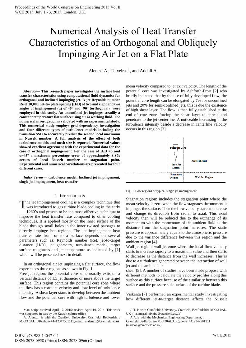
In an orthogonal air jet impinging a flat surface, the flow
experiences three regions as shown in Fig. 1
Free jet region: the potential core zone usually exits on a
vertical distance of 1.5 jet diameter or more above the target
surface. This region contains the potential core zone where
the flow has a constant velocity and low level of turbulence
intensity. A shear layer starts to develop between the ambient
flow and the potential core with high turbulence and lower
Manuscript received April 17, 2015; revised April 19, 2014. This work
was supported in part by the Kuwait culture office . A. Alenezi. is with the Cranfield University, Cranfield, Bedfordshire
MK43 0AL. UK(phone+4412347501111;e-mail: [email protected]
mean velocity compared to jet exit velocity. The length of the
potential core was investigated by Ashforth-Frost [2] who
briefly indicated that by the use of fully developed flow, the
potential core length can be elongated by 7% for unconfined
jets and 20% for semi-confined jets, this is due the existence
of high shear layer. The flow is then fully established at the
end of core zone forcing the shear layer to spread and
penetrate to the jet centerline. A noticeable increasing in the
turbulence intensity beside a decrease in centerline velocity
occurs in this region [3].
Fig 1 Flow regions of typical single jet impingement
Stagnation region: includes the stagnation point where the
mean velocity is zero when the flow stagnates the moment it
impinges the surface. Then the flow velocity starts to increase
and change its direction from radial to axial. This axial
velocity then will be reduced due to the exchange of its
momentum with the momentum of the ambient fluid as the
distance from the stagnation point increases. The static
pressure is approximately equals to the atmospheric pressure
due to the variance difference between this region and the
ambient region [4].
Wall jet region: wall jet zone where the local flow velocity
starts to increase rapidly to a maximum value and then starts
to decrease as the distance from the wall increases. This is
due to a turbulence generated between the interaction of wall
jet and the ambient air
shear [5]. A number of studies have been made propose with
different methods to calculate the velocity profiles along this
surface as this surface because of the similarity between this
surface and the pressure side surface of the turbine blade.
Viskanta [7] performed an experimental study investigating
how different jet-to-target distance affects the Nusselt
J. T. is with Cranfielde University, Cranfield, Bedfordshire MK43 0AL.
UK .([email protected]) A.A.is with the Mechanical Engineering Department, ,
Cranfield,Bedfordshire MK430AL.UK(phone+4412347501111
Numerical Analysis of Heat Transfer
Characteristics of an Orthogonal and Obliquely
Impinging Air Jet on a Flat Plate
Alenezi A., Teixeira J., and Addali A.
T
Proceedings of the World Congress on Engineering 2015 Vol II WCE 2015, July 1 - 3, 2015, London, U.K.
ISBN: 978-988-14047-0-1 ISSN: 2078-0958 (Print); ISSN: 2078-0966 (Online)
WCE 2015
number using a single 0.78 mm in diameter round jet with Re
of 23,000 using different (H/D). In general, stagnation point
has the highest heat transfer coefficient as also indicated by
[5].This observation agreed with results reported from [8] and
[9]. A typical (H/D) value of modern gas turbines differs
between1 to 3 [3].Goldstein and Behbahani [10] reported that
a reduction in heat transfer coefficient peak occurs under the
influence of cross flow and large jet-to-target distance while
at small distances cross flow increases this peak. A secondary
peak was also explained by [11] and [12] as an increase in
local heat transfer coefficient at low jet-to-target distance at
the transition phase between laminar and turbulent flow in
wall jet region. This is due the existence of recirculation
region as also supported by the sub-atmospheric pressure data
[13].
Sagot [14] investigated experimentally the influence of
different jet-to-target distances on the average heat transfer
coefficient using rounded jet nozzle with diameters range
from 2.4 to 8mm. The jet flow temperature ranges between
40 and 65ºC impinging a smooth aluminium flat plate which
was exposed to a fixed temperature of 4ºC under the influence
of different Reynolds numbers between 15,000 and 30,000.
The author reported that, for large jet-to-target distance
(2<H/D<6), the parameter (H/D) has a weak impact on the
average heat transfer coefficient. Miao [15] employed a
confined rounded
jet array impinging orthogonally a flat plate at different cross
flow orientations. He reported that the area-averaged Nusselt
number increases by increasing jet-to-target spacing and
increasing Reynolds number.
Donaldson [16; 17] made a two-part experimental study of
an adjustable axisymmetric jet impinging several surfaces.
Jet-to-target distances varied between 1.96 and 39.1 jet
diameters with jet angle between 30 and 75˚ and 1.25 to 6.75
pressure ratios employing sonic and subsonic jets. Hot wire
and pressure taps were used to measure surface static pressure
and free jet velocity respectively. He conducted that, for H/D
>20, the maximum pressure point located on the target
surface is a function of impingement angle and the jet
pressure ratio almost has no effect. On the other hand, for
closer H/D, the strong relation between the maximum
pressure ratio location and jet angle still exits but the pressure
ratio turned up to be a significant factor. Yan and Saniei [18]
used an oblique circular jet impinging a flat plate with angles
varied between 45º and 90º to investigate the heat transfer
characteristics. Temperature distributions over the preheated
plate was measured using transient liquid crystal technique
adopting Reynolds numbers between 10,000 and 23,000 and
for (H/D) of 4, 7, and 10. Results reported that the point where
the maximum heat transfer occurs is shifted away from the
geometrical point in the direction of the uphill side of the
plate.
Tong [19] in his study investigated numerically the
hydrodynamics and heat transfer rate of an inclined plane jet.
The results show that with uniform flow profile, the
magnitude of the Nusselt number peak increases as increasing
the jet angle from normal position. This peak initially
declines and then start to rise having a parabolic jet flow
profile. His experimental study used an inclined slot jet
impinging liquid on a flat plate to investigate the heat transfer
from a distance of three jet diameter (D = 2mm) with jet
angles of 45º, 60º, 75º, and 90º. Three low Reynolds number
were used of 2500, 5000 and 10,000. He also reported that,
beyond jet-to-target distance (H/D) of 3, there is no more
change in the hydrodynamics heat transfer as shown in
Fig.23. This observation was also reported by the old
theoretical study of Miyazaki [20].
In this research paper, a numerical investigation employing
ANSYS CFD 14.5 code is adapted to study the effect of jet
inclination and jet-to-target distance on the rate of heat
transfer on a flat plate. A Reynolds number of 10,000, a
normalized jet-to-target distance (H/D) of 2 and 8 and finally
two jet inclination angles of (α) of 45° and 90° were
employed in this study. A validation of this numerical study
was made with the experimental data reported from [21].
II. NUMERICAL METHODOLOGY
The commercial tool Ansys Fluent 14.5 was employed in
this study to simulate the jet impingement. Extra attention
was taken on the near-wall region since it plays an important
role for convective heat transfer. This paper aims to improve
the accuracy of the previous numerical studies of jet
impingement heat transfer by accurately resolve the near-wall
boundary layers of the flow. A validation was made by
comparing the results of Nusselt number with experimental
results reported by [21].
A. THE COMPUTATIONAL DOMAIN
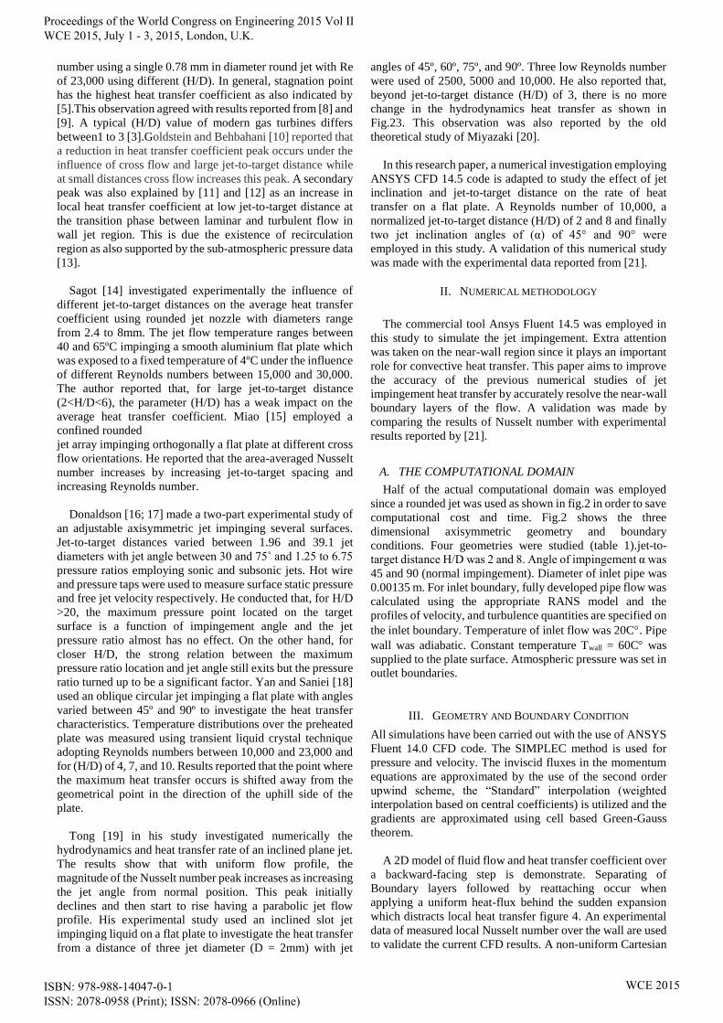
Half of the actual computational domain was employed
since a rounded jet was used as shown in fig.2 in order to save
computational cost and time. Fig.2 shows the three
dimensional axisymmetric geometry and boundary
conditions. Four geometries were studied (table 1).jet-to-
target distance H/D was 2 and 8. Angle of impingement α was
45 and 90 (normal impingement). Diameter of inlet pipe was
0.00135 m. For inlet boundary, fully developed pipe flow was
calculated using the appropriate RANS model and the
profiles of velocity, and turbulence quantities are specified on
the inlet boundary. Temperature of inlet flow was 20C. Pipe
wall was adiabatic. Constant temperature Twall = 60C was
supplied to the plate surface. Atmospheric pressure was set in
outlet boundaries.
III. GEOMETRY AND BOUNDARY CONDITION
All simulations have been carried out with the use of ANSYS
Fluent 14.0 CFD code. The SIMPLEC method is used for
pressure and velocity. The inviscid fluxes in the momentum
equations are approximated by the use of the second order
upwind scheme, the “Standard” interpolation (weighted
interpolation based on central coefficients) is utilized and the
gradients are approximated using cell based Green-Gauss
theorem.
A 2D model of fluid flow and heat transfer coefficient over
a backward-facing step is demonstrate. Separating of
Boundary layers followed by reattaching occur when
applying a uniform heat-flux behind the sudden expansion
which distracts local heat transfer figure 4. An experimental
data of measured local Nusselt number over the wall are used
to validate the current CFD results. A non-uniform Cartesian
Proceedings of the World Congress on Engineering 2015 Vol II WCE 2015, July 1 - 3, 2015, London, U.K.
ISBN: 978-988-14047-0-1 ISSN: 2078-0958 (Print); ISSN: 2078-0966 (Online)
WCE 2015
mesh sizing 121X61 was adopted in this simulation. A fully
developed, steady and incompressible flow with constant
properties ware used as inlet boundary conditions. The
thickness of the incoming boundary layer is 1.1H Figure 1a.
Employing the standard wall functions RNG k-ε turbulent
model to account for turbulence behavior with Reynolds
number Re=28,000.
TABLE I PARAMETERS OF GEOMETRY
case H/D α,
1 6 90
2 6 45
3 2 90
4 2 45
A. MESH GENERATION:
In order to resolve the flow features for different H/D and
jet angles, a very fine hexahedral mesh was employed in this
simulation using grid refinement inside the wall boundary
layer. The used mesh is intended to accurately determine the
flow parameters as a function of the simulation parameters,
grid refinement for boundary layers neighboring the wall is a
suitable approach to be use. Generating and then modifying
the hexahedral mesh topology to ensure domain orthogonality
by first using a course mesh scheme then modifying the mesh
to control on the physics distance of the first node from the
wall ( 𝑦+). Keeping the 𝑦+ equals or below 0.5 for the near-
wall cells is an important step to resolve the viscous laminar
sublayer which needs at least 12 nodes. The final mesh is
designed to have nodes near the target surface where jet
mixing occurs.
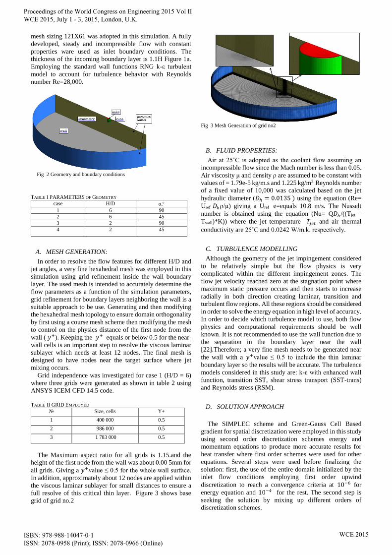
Grid independence was investigated for case 1 (H/D = 6)
where three grids were generated as shown in table 2 using
ANSYS ICEM CFD 14.5 code.
TABLE II GRID EMPLOYED
№ Size, cells Y+
1 400 000 0.5
2 986 000 0.5
3 1 783 000 0.5
The Maximum aspect ratio for all grids is 1.15.and the
height of the first node from the wall was about 0.00 5mm for
all grids. Giving a 𝑦+value ≤ 0.5 for the whole wall surface.
In addition, approximately about 12 nodes are applied within
the viscous laminar sublayer for small distances to ensure a
full resolve of this critical thin layer. Figure 3 shows base
grid of grid no.2
Fig 3 Mesh Generation of grid no2
B. FLUID PROPERTIES:
Air at 25˚C is adopted as the coolant flow assuming an
incompressible flow since the Mach number is less than 0.05.
Air viscosity μ and density ρ are assumed to be constant with
values of = 1.79e-5 kg/m.s and 1.225 kg/m3. Reynolds number
of a fixed value of 10,000 was calculated based on the jet
hydraulic diameter (𝐷ℎ = 0.0135 ) using the equation (Re=
Uref 𝐷ℎρ/μ) giving a Uref e=equals 10.8 m/s. The Nusselt
number is obtained using the equation (Nu= Q𝐷ℎ/((Tjet –
Twall)*K)) where the jet temperature 𝑇𝑗𝑒𝑡 and air thermal
conductivity are 25˚C and 0.0242 W/m.k. respectively.
C. TURBULENCE MODELLING
Although the geometry of the jet impingement considered
to be relatively simple but the flow physics is very
complicated within the different impingement zones. The
flow jet velocity reached zero at the stagnation point where
maximum static pressure occurs and then starts to increase
radially in both direction creating laminar, transition and
turbulent flow regions. All these regions should be considered
in order to solve the energy equation in high level of accuracy.
In order to decide which turbulence model to use, both flow
physics and computational requirements should be well
known. It is not recommended to use the wall function due to
the separation in the boundary layer near the wall
[22].Therefore; a very fine mesh needs to be generated near
the wall with a 𝑦+value ≤ 0.5 to include the thin laminar
boundary layer so the results will be accurate. The turbulence
models considered in this study are: k-ε with enhanced wall
function, transition SST, shear stress transport (SST-trans)
and Reynolds stress (RSM).
D. SOLUTION APPROACH
The SIMPLEC scheme and Green-Gauss Cell Based
gradient for spatial discretization were employed in this study
using second order discretization schemes energy and
momentum equations to produce more accurate results for
heat transfer where first order schemes were used for other
equations. Several steps were used before finalizing the
solution: first, the use of the entire domain initialized by the
inlet flow conditions employing first order upwind
discretization to reach a convergence criteria at 10−6 for
energy equation and 10−4 for the rest. The second step is
seeking the solution by mixing up different orders of
discretization schemes.
Fig 2 Geometry and boundary conditions
Proceedings of the World Congress on Engineering 2015 Vol II WCE 2015, July 1 - 3, 2015, London, U.K.
ISBN: 978-988-14047-0-1 ISSN: 2078-0958 (Print); ISSN: 2078-0966 (Online)
WCE 2015
IV. SENSITIVITY ANALYSIS
The next sub-sections introduce an inclusive analysis of
both models and parameters when employing the numerical
model. An intensive discussion in each sub-section is carried
out for CFD mythology aspect and validated with
experimental data in [21]. For clarification, only one
comparison to the experimental data was performed
employing k-ε turbulence model, Re=10,000, α=90˚and
H/D=6 to specify the appropriate grid size to use for the rest
of simulations. In all following figures, experimental data are
signified by line with triangles marks. The effects of jet
angles (α) and jet-to-target distances (H/D) on the heat
transfer rate will be discussed in section 4.
A. DISCRETIZATION SCHEME
To increase the results accuracy of heat convection in jet
impingement, a higher order discretization scheme must be
adapted. A succeeding enhancement from the first to second
order discretization scheme improves the numerical heat
transfer rate compared to the experimental values. In order to
capture the secondary peak in Nusselt number (Nu)
distribution which occurs at a certain radial distance from the
stagnation point, a second order scheme should be employed
on the domain. The first order scheme however, is not
consistent with the experimental data for short radial distance
r/D<2 where the laminar-turbulence transition region occurs.
B. GRID REFINMENET STUDY
A grid analysis is employed in this study to certify that the
solution is independent of the computational grid. Generally,
both numerical solution accuracy and numerical time depend
mainly on mesh refinement. In this work, the suitable grid is
examined to have the proper run-time and accuracy. Three
grid cases considered in the present grid refinement study, as
shown in table 2. Figure 4 shows values of Nusselt number
varied with the radial distance r/D under the influence of k-ε
turbulence model, H/D=6 and jet angle of 90˚ for different
grids. It is notable, that both experimental and the numerical
local Nusselt number values are close for all grid cases and
therefore, grid 2 will be used for the rest of the numerical
cases.
Fig 4 Nusselt number distribution for three types of grids
C. CODE VALIDATION
To validate the numerical results, the local Nusselt number
Nu is compared to the benchmark experimental data by
O’Donovan and Murray [21] for four different turbulence
models. Comparison between results is shown in figure 5. As
shown in this figure, for an orthogonal jet with H/D=6, the k-
ε turbulence model shows an excellent agreement with the
experimental data comparing to the other three turbulence
models. Therefore, the k-ε turbulence model will be used for
all simulation cases.
Fig 5 Local Nusselt number Vs r/D for four different turbulence models
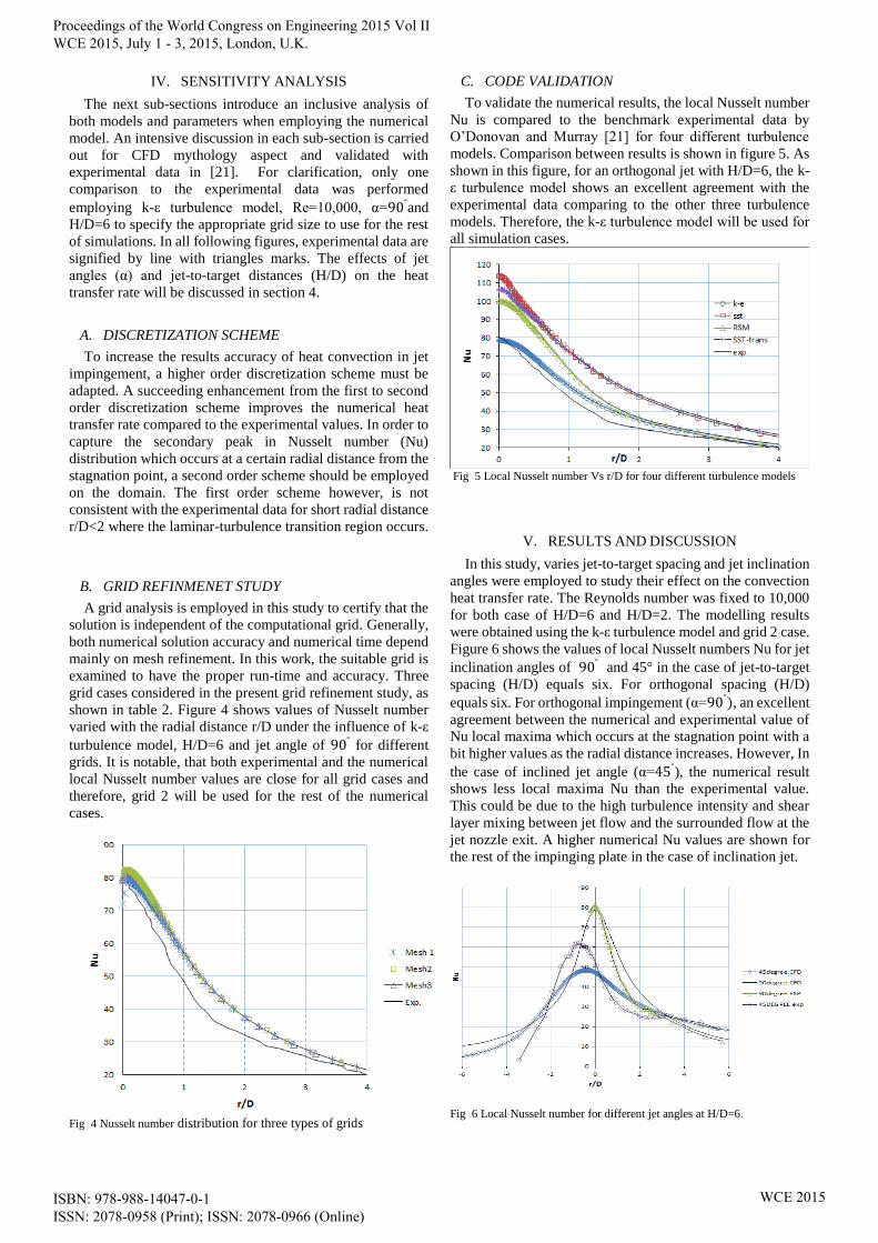
V. RESULTS AND DISCUSSION
In this study, varies jet-to-target spacing and jet inclination
angles were employed to study their effect on the convection
heat transfer rate. The Reynolds number was fixed to 10,000
for both case of H/D=6 and H/D=2. The modelling results
were obtained using the k-ε turbulence model and grid 2 case.
Figure 6 shows the values of local Nusselt numbers Nu for jet
inclination angles of 90˚ and 45° in the case of jet-to-target
spacing (H/D) equals six. For orthogonal spacing (H/D)
equals six. For orthogonal impingement (α=90˚), an excellent
agreement between the numerical and experimental value of
Nu local maxima which occurs at the stagnation point with a
bit higher values as the radial distance increases. However, In
the case of inclined jet angle (α=45˚), the numerical result
shows less local maxima Nu than the experimental value.
This could be due to the high turbulence intensity and shear
layer mixing between jet flow and the surrounded flow at the
jet nozzle exit. A higher numerical Nu values are shown for
the rest of the impinging plate in the case of inclination jet.
Fig 6 Local Nusselt number for different jet angles at H/D=6.
Proceedings of the World Congress on Engineering 2015 Vol II WCE 2015, July 1 - 3, 2015, London, U.K.
ISBN: 978-988-14047-0-1 ISSN: 2078-0958 (Print); ISSN: 2078-0966 (Online)
WCE 2015

Figure 7 illustrates the same study discussed in the last
paragraph but for a closer jet-to-target spacing (H/D=2). It is
noticeable that the overall values of local Nusselt numbers for
both numerical and experimental increase by decreasing the
jet-to-target spacing due to less turbulence intensity and
higher jet arrival velocity. For orthogonal jet, the numerical
local Nusselt number values show higher in magnitude than
the experimental values for all radial distances except for
r/D≥2 where both values become to be much closer. This is
not the case for the inclination jet, where the experimental
values of local Nusselt number are higher at the stagnation
point and then become lower for the rest of the radial
distances
Fig 7 Local Nusselt number for different angles at H/D=2
Figures 8a and 8b show the velocity magnitude distributions
of the orthogonal jet for H/D=6 and H/D=2 respectively.
Comparing the value of the arrival velocity for both cases, it
can be noticed that as the H/D increases, the arrival jet
velocity decreases and the turbulence intensity increases
Fig 8 Velocity distributions of orthogonal jet for a) H/D=6 , b) H/D=2
Figures 9 a and b show the velocity magnitude distribution
of a jet angle (α=45˚) where the stagnation point is different
from the geometric center. The arrival jet velocity in the case
of lower jet-to-target spacing is higher in magnitude than it in
the case of higher jet-to-target spacing. On the other hand, the
turbulence intensity is lower for lower H/D.
Fig 9 Velocity distributions of inclined jet for a) H/D=6 , b) H/D=2
VI. CONCLUSION
The use of k-ε turbulence model saves computational time
and cost with accurate results in prediction the heat transfer
rate when compared to the detailed experimental results for
validation. Furthermore, all physics properties of both the jet
and the heated plate accurately calculated by adapting grid
density in the near-wall region. Results reported from this
study were captured using Re=10,000, jet-to-target spacing
H/D between two and six. The values of the dimensionless
distance between the wall and the first node (𝑦+) and Prandtl
number in the near-wall region have proven to be important
parameters in predicting the turbulent heat transfer since their
values effect directly the heat diffusion level. Interestingly
enough that all the four turbulent models used in this study
have failed to predict the secondary peak of Nusselt number
which supposed to occur at approximately r/D=3. Alternative
turbulent models such as Large Eddy Simulation (LES) or
Detached Eddy Simulation (DES) can be used such in order
to predict the Nusselt number secondary peak.
The use of accurate boundary conditions including fluid
properties, appropriate computational domain, and the right
solution approach has been proven to be the main parameters
in order to accurately predict the heat transfer rate for circular
jet impingement.
REFERENCES
[1] Jambunathan, K., Lai, E., Moss, M. A. and Button, B. L. (1992),
"Areview of heat transfer data for single circular jet impingement",International Journal of Heat and Fluid Flow, vol. 13,
no. 2, pp. 106-115.
[2] Ashforth-Frost, S. and Jambunathan, K. (1996), "Effect of nozzle [3] geometry and semi-confinement on the potential core of a turbulent
axisymmetric free jet", international Communications in Heat and
Mass Transfer, vol. 23, pp. 155-162. [4] O’Donovan, T. S., and Murray, D. B., 2007, “Jet Impingement Heat
Transfer— Part I: Mean and Root-Mean-Square Heat Transfer and
Velocity Distributions,”B. Smith, “An approach to graphs of linear forms (Unpublished work style),” unpublished.
[5] Livingood, J., N. B. and Hryack, P. (1973), "impingement heat transfer
from turbulent air jets to flat plates", NASA TM X-2778, J. [6] Zuckerman, N. and Lior, N. (2005), "Impingement Heat Transfer:
Correlations and Numerical Modeling", Journal of Heat Transfer, vol.
127, no. 5, pp. 544-552. [6] Donaldson, C. D., and Snedeker, R. S., 1971, \A study of free jet impingement, part i mean properties of free
impinging jets," Journal of Fluid Mechanics, 45, pp. 281-319.
[7] Viskanta, R. (1993), "Heat Transfer to impinging isothermal gas and [8] Hollworth, B. R. and Wilson, S. I. (1984), "Entrainment Effects on
Impingement Heat Transfer.Part 1 Measurments of Heat Jet Velocity
and Temperature Distributions and Recovery Temperatures on Target Surfaces", J. of Heat Transfer, vol. 106, pp. 797-803
[9] Sparrow, E. M. and Lovell, B. J. (1980), "Heat Transfer Characteristics
of an Obliquely Impinging Circular Jet", J. Heat Transfer, vol. 102, pp. 202-209.
[10] Goldstein, R. J. and Behbahani, A. I. (1982), "Impingement of a
circular jet with and without cross flow", Int. J. Heat Mass Transfer, vol. 25, no 9, pp. 1377-1382.
Proceedings of the World Congress on Engineering 2015 Vol II WCE 2015, July 1 - 3, 2015, London, U.K.
ISBN: 978-988-14047-0-1 ISSN: 2078-0958 (Print); ISSN: 2078-0966 (Online)
WCE 2015

[11] Lytle, D. and Webb, B. W. (1994), "Air jet impingement heat transfer
at low nozzle-plate spacings", Int. J. Heat Mass Transfer,no. 12, pp. 1687-1697.R. W. Lucky, “Automatic equalization for digital
communication,” Bell Syst. Tech. J., vol. 44, no. 4, pp. 547–588, Apr.
1965. [12] Walker, D. A. and Smith, C. R. (1987), "The impact of a vortex ring on
a wall", J. Fluid Mech., vol. 181, pp. 99-140G. R. Faulhaber, “Design
of service systems with priority reservation,” in Conf. Rec. 1995 IEEE Int. Conf. Communications, pp. 3–8.
[13] Colucci, D. W. and Viskanta, R. (1996), "Effect of nozzle geometry on local convective heat transfer to a confined impinging air jet",
Experimental Thermal and Fluid Science, vol. 13, no. 1, pp. 71-80G. W. Juette and L. E. Zeffanella, “Radio noise currents n short sections
on bundle conductors (Presented Conference Paper style),” presented
at the IEEE Summer power Meeting, Dallas, TX, Jun. 22–27, 1990, Paper 90 SM 690-0 PWRS.
[14] Sagot, B., Antonini, G., Christgen, a. and Buron, F. (2008), "Jet
[15] Impingement heat transfer on a flat plate at a constant wall temperature", International Journal of Thermal Sciences, vol. 47, no.
12, pp. 1610-1619.
[16] Donaldson, C., Snedeker, R. and Margolis, P. (1971), "A study of jet
impingement. Part 2. Free jet turbulent structure and impingement heat
transfer", J. Fluid Mech., vol. 45, no. 3, pp. 477-512.
[17] Donaldson, C. and Snedeker, R. (1971), "A study of free jet Impingement. Part 1. Mean properties of free and impinging jets", J.
Fluid Mech., vol. 45, no. 2, pp. 281-319.
[18] Yan, X. and Saniei, N. (1997), "Heat transfer from an obliquely impinging circular, air jet to a flat plate", International Journal of Heat
and Fluid Flow, vol. 18, no. 6, pp. 591-599.
[19] Tong, A. Y. (2003), "On the impingement heat transfer of an oblique free surface plane jet", International Journal of Heat and Mass Transfer,
vol. 46, no. 11, pp. 2077-2085
[20] Miyazaki, H. and Silberman, E. (1972), "Flow and heat transfer on a flat plate normal to a two-dimensional laminar jet issuing from a nozzle
of finite height", International Journal of Heat and Mass Transfer, vol.
15, no. 11,pp. 2097-2107. [21] O’Donovan, T. and Murray, D. (2008), “Fluctuating fluid flow and heat
transfer of an obliquely impinging air jet” International Journal of Heat
and Mass Transfer 51 (2008) 6169–6179pp. 2097-2107. [22] Hadziabdic, M., and Hanjalic, K., 2008, “Vortical Structures and Heat
Transfer in a Round Impinging Jet,” J. Fluid Mech., 596, pp. 221–260
[23] O’Donovan, 2005, FLUID FLOW AND HEAT TRANSFER OF AN IMPINGING AIR JET. PhD thesis, University of Dublin
Proceedings of the World Congress on Engineering 2015 Vol II WCE 2015, July 1 - 3, 2015, London, U.K.
ISBN: 978-988-14047-0-1 ISSN: 2078-0958 (Print); ISSN: 2078-0966 (Online)
WCE 2015