Numerical Analysis of a Rotating Detonation Engine in … E. Paxson Glenn Research Center,...

Daniel E. PaxsonGlenn Research Center, Cleveland, Ohio

Numerical Analysis of a Rotating Detonation Engine in the Relative Reference Frame

NASA/TM—2014-216634

March 2014

AIAA–2014–0284

https://ntrs.nasa.gov/search.jsp?R=20140013391 2018-07-01T14:26:57+00:00Z

��

�� !�� "��#�"��

�� "�$�� %��&�� '�� (��)��*��)��+��"��)��*��*��"��, .� �5$7��$�9��:;9�$��%��)��

� �� <�� =��"�� +��*�� =��

.� �5$7��$�9�>5>%)��(:>��

�� "�� &��?��#�� *#�� (��=��"��

.� $%��)�$�%)�)5�%)��

��"��+��

.� $%�@5)5�$5��:;9�$��%��$�� " �� "��

.� ��5$��9��:;9�$��%��

�� <�� *��<��

.� �5$7��$�9��)��9��%��5��+

�� '��

��&�� &��&��

@� �� *��,

.� �� http://www.sti.nasa.gov

.� 5+ ��"��?��[email protected] .� @�=�"��?��

�� (��#��BBCGHJHGJKLC .� �� (��#�� BBCGHJHGJKLO .� P��,

�� (��# ��$�� HQQJ��(��7��>(�OQLHUGQCOL

Daniel E. PaxsonGlenn Research Center, Cleveland, Ohio


NASA/TM—2014-216634

March 2014

AIAA–2014–0284

��

V��)��$�� $��%��BBQCJ

��OLQB��"�� 7��>�"��W��"�QCGQH��OLQB

��

��$�� HQQJ��(��7��>(�OQLHUGQCOL

�� JCLQ��*��)��

��=��X��OOCQO

��"��,YY***��

Level of Review,�� "��*��"��

�� *#��

��

�� "��<��"��

NASA/TM—2014-216634 1


Daniel E. Paxson

National Aeronautics and Space Administration Glenn Research Center Cleveland, Ohio 44135

Abstract A two-dimensional, computational fluid dynamic (CFD) simulation of a semi-idealized rotating

detonation engine (RDE) is described. The simulation operates in the detonation frame of reference and utilizes a relatively coarse grid such that only the essential primary flow field structure is captured. This construction yields rapidly converging, steady solutions. Results from the simulation are compared to those from a more complex and refined code, and found to be in reasonable agreement. The performance impacts of several RDE design parameters are then examined. Finally, for a particular RDE configuration, it is found that direct performance comparison can be made with a straight-tube pulse detonation engine (PDE). Results show that they are essentially equivalent.

Nomenclature

a non-dimensional speed of sound a* dimensional reference speed of sound AFR air to fuel ratio (by mass) � ratio of inlet (or exit) slit height to annulus height F non-dimensional conserved circumferential flux vector gc Newton constant G non-dimensional conserved axial flux vector � ratio of specific heats hf fuel heating value I impulse K0 non-dimensional reaction rate constant l circumferential length L tube length My axial Mach number p non-dimensional pressure p* dimensional reference pressure q0 non-dimensional heat addition parameter Rg real gas constant { non-dimensional density {* dimensional reference density S non-dimensional source term vector T non-dimensional temperature T* dimensional reference temperature Tc0 non-dimensional reaction temperature Tsp specific thrust t non-dimensional time u non-dimensional circumferential velocity v non-dimensional axial velocity w non-dimensional conserved state vector

NASA/TM—2014-216634 2

x non-dimensional circumferential distance y non-dimensional axial distance z reactant fraction Subscripts e exit plane b back (as in back or ambient pressure) det referring to the detonation tr total (pressure or temperature) in reservoir

1.0 Introduction The rotating detonation engine (RDE) represents an intriguing approach to achieving pressure gain

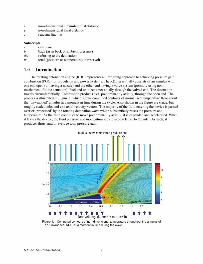
combustion (PGC) for propulsion and power systems. The RDE essentially consists of an annulus with one end open (or having a nozzle) and the other end having a valve system (possibly using non-mechanical, fluidic actuation). Fuel and oxidizer enter axially through the valved end. The detonation travels circumferentially. Combustion products exit, predominantly axially, through the open end. The process is illustrated in Figure 1, which shows computed contours of normalized temperature throughout the ‘unwrapped’ annulus at a moment in time during the cycle. Also shown in the figure are crude, but roughly scaled inlet and exit axial velocity vectors. The majority of the fluid entering the device is passed over or ‘processed’ by the rotating detonation wave which substantially raises the pressure and temperature. As the fluid continues to move predominantly axially, it is expanded and accelerated. When it leaves the device, the fluid pressure and momentum are elevated relative to the inlet. As such, it produces thrust and/or average total pressure gain.

Figure 1.—Computed contours of non-dimensional temperature throughout the annulus of

an ‘unwrapped’ RDE, at a moment in time during the cycle.

x/l

y/l

0 0.1 0.2 0.3 0.4 0.5 0.6 0.7 0.8 0.9 10

0.1

0.2

0.3

0.4

2

4

6

8

10

detonation direction

low velocity detonable mixture in

high velocity combustion products out

detonation

y

x

NASA/TM—2014-216634 3

The potential advantages of this approach compared to conventional pulsed detonation engines (PDE’s) include the elimination of initiation and deflagration to detonation transition (DDT) devices, and an exceptionally high cycle rate governed by the transit time of the detonation around the circumference.

Although these devices have been demonstrated in the laboratory (Refs. 1 and 2), they are difficult to instrument. Additionally, since nearly all laboratory devices do not have mechanical valves, they cannot be safely operated with premixed fuel and air. As such there is significant uncertainty about local stoichiometry and therefore detonation properties. The net result of these difficulties is that, while RDE’s are operational, their fundamental physical principles are not well understood. Not surprisingly, neither are methodologies to optimize performance.

Computational fluid dynamic (CFD) studies have been performed (Refs. 3 and 4); however, they are relatively few in comparison to those for PDE’s. As such there is a need for further and varied computational studies in order to compare against each other, and with the growing body of experiments. Furthermore, many of the existing computational models are constructed with the goal of capturing tremendous detail in the flow field. This implies fine grid spacing, and complex reaction models that, while yielding valuable data, require vast computational resources and time in order to reach convergence. For the sort of parametric evaluations needed to understand fundamental operational physics, a simpler, less refined modeling approach is beneficial.

This paper presents the preliminary results of just such an approach. A CFD-based RDE model is described whereby the reference frame of the rotating detonation is adopted. As such, converged solutions are obtained which are steady in time. This is insured by utilizing a relatively coarse grid and a simple finite rate reaction model which respectively eliminate the otherwise unstable shear flow, and the cellular detonation structure associated with more detailed analyses. Comparison with the more detailed CFD models will show that these simplifications preserve performance prediction capability, and by extension, the capture of essential RDE physics. The use of a coarse grid also yields converged solutions rapidly while utilizing modest computational resources. This feature makes the model useful for parametric studies related to performance.

The flexibility of the model, and its methodological similarity to a quasi-one-dimensional CFD code for investigating conventional pulse detonation engines (PDE) (Ref. 5), allow for a direct comparison of semi-idealized RDE and PDE performance. The conditions under which this comparison is made, and the results will be described. The results will show that under these conditions, the performance of RDE’s and PDE’s is nearly the same.

A simplified configuration of the model will also be described which is used to investigate explanations for the reduced detonation speeds (compared to one-dimensional theory) observed in experiments. It will be shown that the lack of axial confinement associated with RDE’s is one possibility.

2.0 Model Description The model is developed with the assumption that the working fluid is a calorically perfect gas (CPG)

of fixed composition. This is a significant simplification which is far from reality, particularly in the vicinity of rotating detonation itself. However, it has been shown that with judiciously chosen average gas properties (Ref. 6), remarkably good agreement with experiments can be obtained. More importantly however, the simplification does not fundamentally impact performance trends or fundamental physics, the capture of which are the goals of the present effort. In addition, the CPG assumption greatly simplifies the mathematics associated with code development.

2.1 Governing Equations

On the further assumptions that working fluid is inviscid and adiabatic, and that the RDE annulus radius of curvature is much greater than its height, the governing equations of motion may be written in non-dimensional form as follows.

NASA/TM—2014-216634 4

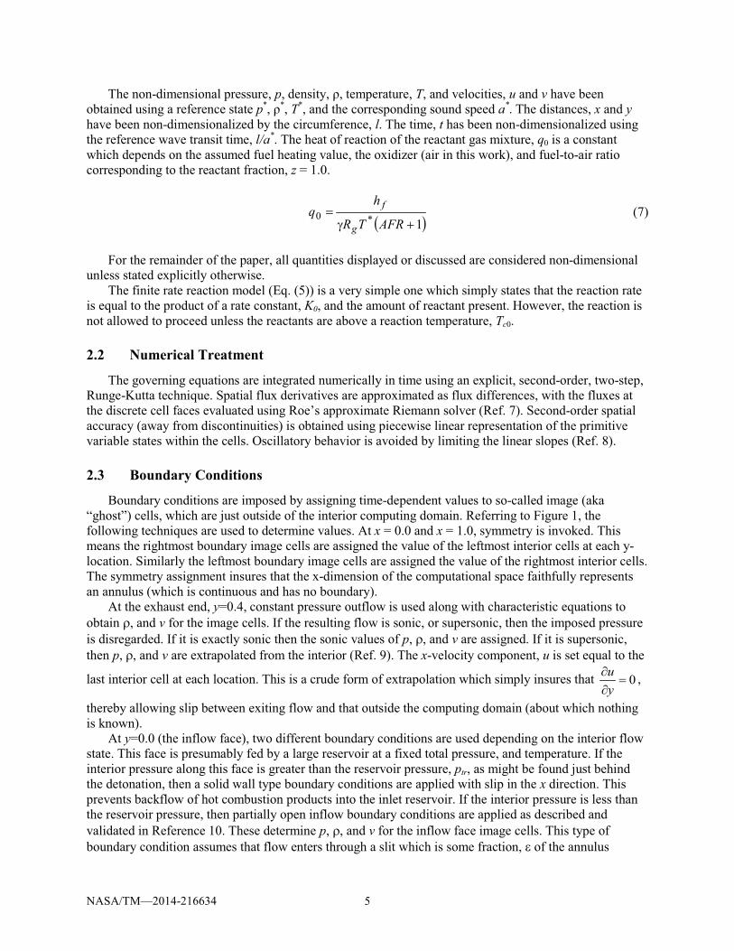
S = yG

xF +

tw

��

��

�� (1)

where

� ��

��

��

�

�

��

��

��

z

vupvu

21

= w 22 (2)

� ��

��

�

�

��

��

� ��

�

��

�

uz

vu

uv

u

u

2 +

1)(pu

+ p

= F22

2

(3)

� �

��

��

�

�

��

��

� ��

��

��

vz

vuv

v

uvv

G

2 +

1)(p

+ p

=

22

2 (4)

��

��

�

��

��

��

��

��

��

��

��

0

00

0

000

;0;

;0;000

c

c

c

c

TTTTK

z

TTTTK

zqS (5)

The non-dimensional equation of state needed to complete the governing equation set is written as follows.

Tp �� (6)

NASA/TM—2014-216634 5

The non-dimensional pressure, p, density, {, temperature, T, and velocities, u and v have been obtained using a reference state p*, {*, T*, and the corresponding sound speed a*. The distances, x and y have been non-dimensionalized by the circumference, l. The time, t has been non-dimensionalized using the reference wave transit time, l/a*. The heat of reaction of the reactant gas mixture, q0 is a constant which depends on the assumed fuel heating value, the oxidizer (air in this work), and fuel-to-air ratio corresponding to the reactant fraction, z = 1.0.

� �1*0

��

AFRTR

hq

g

f (7)

For the remainder of the paper, all quantities displayed or discussed are considered non-dimensional unless stated explicitly otherwise.

The finite rate reaction model (Eq. (5)) is a very simple one which simply states that the reaction rate is equal to the product of a rate constant, K0, and the amount of reactant present. However, the reaction is not allowed to proceed unless the reactants are above a reaction temperature, Tc0.

2.2 Numerical Treatment

The governing equations are integrated numerically in time using an explicit, second-order, two-step, Runge-Kutta technique. Spatial flux derivatives are approximated as flux differences, with the fluxes at the discrete cell faces evaluated using Roe’s approximate Riemann solver (Ref. 7). Second-order spatial accuracy (away from discontinuities) is obtained using piecewise linear representation of the primitive variable states within the cells. Oscillatory behavior is avoided by limiting the linear slopes (Ref. 8).

2.3 Boundary Conditions

Boundary conditions are imposed by assigning time-dependent values to so-called image (aka “ghost”) cells, which are just outside of the interior computing domain. Referring to Figure 1, the following techniques are used to determine values. At x = 0.0 and x = 1.0, symmetry is invoked. This means the rightmost boundary image cells are assigned the value of the leftmost interior cells at each y-location. Similarly the leftmost boundary image cells are assigned the value of the rightmost interior cells. The symmetry assignment insures that the x-dimension of the computational space faithfully represents an annulus (which is continuous and has no boundary).

At the exhaust end, y=0.4, constant pressure outflow is used along with characteristic equations to obtain �, and v for the image cells. If the resulting flow is sonic, or supersonic, then the imposed pressure is disregarded. If it is exactly sonic then the sonic values of p, �, and v are assigned. If it is supersonic, then p, �, and v are extrapolated from the interior (Ref. 9). The x-velocity component, u is set equal to the

last interior cell at each location. This is a crude form of extrapolation which simply insures that 0��

yu ,

thereby allowing slip between exiting flow and that outside the computing domain (about which nothing is known).

At y=0.0 (the inflow face), two different boundary conditions are used depending on the interior flow state. This face is presumably fed by a large reservoir at a fixed total pressure, and temperature. If the interior pressure along this face is greater than the reservoir pressure, ptr, as might be found just behind the detonation, then a solid wall type boundary conditions are applied with slip in the x direction. This prevents backflow of hot combustion products into the inlet reservoir. If the interior pressure is less than the reservoir pressure, then partially open inflow boundary conditions are applied as described and validated in Reference 10. These determine p, �, and v for the inflow face image cells. This type of boundary condition assumes that flow enters through a slit which is some fraction, � of the annulus

NASA/TM—2014-216634 6

height. The slit may be imagined as an infinitesimally short converging nozzle. The flow between the reservoir and the nozzle throat is isentropic. For values of � < 1 however, there is a total pressure mixing loss that takes place across a notional mixing plane separating the nozzle throat from the interior computing domain. In the mixing plane, the magnitude of the total pressure loss varies with the flow rate through the slit and the value of �.

The x-velocity component, u, is prescribed during inflow, and it is here that a reference frame change is implemented. Rather than specify u=0 (i.e., no swirl) which is the laboratory or fixed frame condition, the negative of the detonation speed, udet is prescribed instead. As a result of this change to the detonation reference frame, the computational space becomes one where a steady-state solution is possible. This is the computational equivalent to placing an aircraft model in a wind tunnel and moving the air rather than the model.

2.4 Solution Procedure

The detonation speed is not known a priori. The classical calculation associated with the so-called Chapman-Jouguet (CJ) point is no longer reliable, as it is based on the assumption of strictly one-dimensional flow (with heat addition (Ref. 11). As such, an initial guess is made for udet and steady cold flow is established in the domain. The value of q0 is temporarily set to zero, allowing the potential for reaction without heat release. A steady heat addition rate prescribed at x=0.5, and extending from y=0 to y=0.1 is then applied. The simulation is restarted (from the established cold flow state), and run until steady state is again reached. This step allows the internal flow to become heated, thereby allowing the reaction to proceed, even though the heat release rate (and location) is fixed. At this point, the fixed heat addition rate is turned off, and q0 is restored to the value corresponding to the fuel/oxidizer mixture of interest. The simulation is then restarted and run for the amount of time corresponding to three annular revolutions of the detonation at the assumed detonation speed. The domain is then examined and if it is seen that the detonation front has moved to the right of x=0.5, then it is apparent that the initial guess at udet is too high. If the detonation front has moved to the left, then the initial guess is too low. Based on this determination, a new guess is made for udet, and the simulation is re-run for another three detonation revolutions. The process continues until the detonation front remains stationary and the entire domain stops changing. Because the simulation is typically only 200×80 numerical cells (several orders of magnitude coarser than previous work (Refs. 3 and 4), this can be accomplished in only minutes on a modern laptop computer. When the simulation appears converged, it is then run for the equivalent of 10 additional cycles as a check on whether the detonation is stationary. After this the total mass and energy fluxes at boundaries are checked to insure conservation (i.e., that residuals are acceptably small).

2.5 Deflagration and Detonation Zones

As illustrated in Figure 1, the primary heat release mechanism in an RDE is a detonation. However, there is also a region where deflagration occurs. In the absence of a so-called buffer layer (pure air with no fuel) premixed charge is introduced adjacent to hot combustion products. If the flow field, and numerical approximation thereof, were truly inviscid, no reaction would occur in this region. In real flows however, there is always diffusion; and the best CFD schemes cannot completely avoid numerical diffusion even when physical diffusion terms are neglected. Diffusion results in combustion products heating the premixed charge, thereby allowing the chemical reaction to proceed.

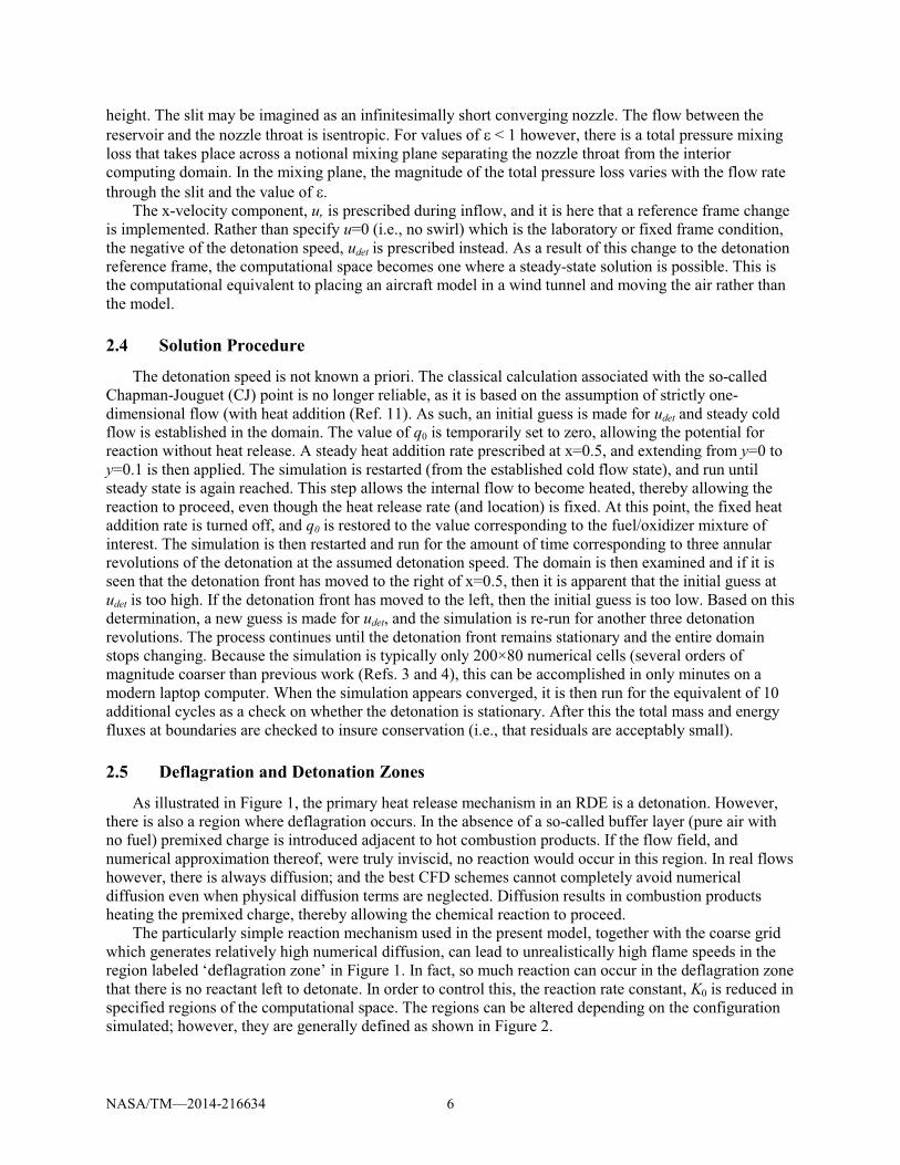
The particularly simple reaction mechanism used in the present model, together with the coarse grid which generates relatively high numerical diffusion, can lead to unrealistically high flame speeds in the region labeled ‘deflagration zone’ in Figure 1. In fact, so much reaction can occur in the deflagration zone that there is no reactant left to detonate. In order to control this, the reaction rate constant, K0 is reduced in specified regions of the computational space. The regions can be altered depending on the configuration simulated; however, they are generally defined as shown in Figure 2.

NASA/TM—2014-216634 7

Figure 2.—Deflagration and detonation zones in the computing domain

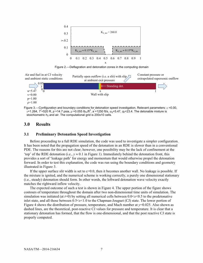
Figure 3.—Configuration and boundary conditions for detonation speed investigation. Relevant parameters: � =0.00,

�=1.264, T*=520 R, p*=14.7 psia, �*=0.055 lbm/ft3, a*=1250 ft/s, ucj=5.47, q0=23.4. The detonable mixture is stoichiometric h2 and air. The computational grid is 200x10 cells.

3.0 Results

3.1 Preliminary Detonation Speed Investigation

Before proceeding to a full RDE simulation, the code was used to investigate a simpler configuration. It has been noted that the propagation speed of the detonation in an RDE is slower than in a conventional PDE. The reasons for this are not clear; however, one possibility may be the lack of confinement at the ‘top’ of the RDE detonation (i.e., y � 0.1 in Figure 1). Immediately behind the detonation front, this provides a sort of ‘leakage path’ for energy and momentum that would otherwise propel the detonation forward. In order to test this explanation, the code was run using the boundary conditions and geometry illustrated in Figure 3.

If the upper surface slit width is set to �=0.0, then it becomes another wall. No leakage is possible. If the mixture is ignited, and the numerical scheme is working correctly, a purely one dimensional stationary (i.e., steady) detonation should form. In other words, the leftward detonation wave velocity exactly matches the rightward inflow velocity.

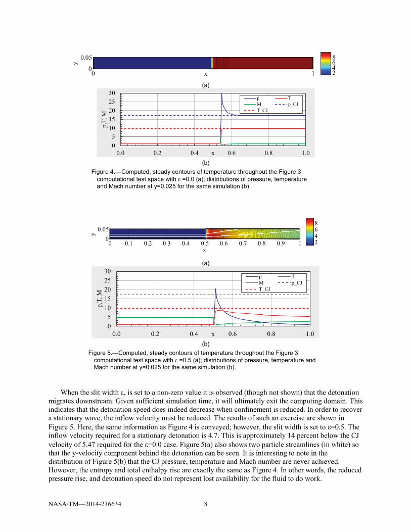
The expected outcome of such a test is shown in Figure 4. The upper portion of the figure shows contours of temperature throughout the domain after two non-dimensional time units of simulation. The simulation was initiated (at t=0) by setting all numerical cells between 0.0<x<0.5 to the predetonative inlet state, and all those between 0.5<x<1.0 to the Chapman-Jouguet (CJ) state. The lower portion of Figure 4 shows the distribution of pressure, temperature, and Mach number at y=0.025. Also shown as dashed lines, are the theoretical, post-reactive CJ values for pressure and temperature. It is clear that a stationary detonation has formed, that the flow is one-dimensional, and that the post reactive CJ state is properly computed.

0

0.1

0.2

0.3

0.4

0 0.1 0.2 0.3 0.4 0.5 0.6 0.7 0.8 0.9 1y

x

K0_def � 0.15*K0_det

K0_det = 260.0

K0_def � 0.15*K0_det

Air and fuel in at CJ velocityand ambient static conditions

Wall with slip

Partially open outflow (i.e. a slit) with slip at ambient exit pressure

Constant pressure or extrapolated supersonic outflow

Standing det.x

y100

0.05

u=5.47v=0.00p=1.00�=1.00

NASA/TM—2014-216634 8

(a)

(b)

Figure 4.—Computed, steady contours of temperature throughout the Figure 3 computational test space with � =0.0 (a); distributions of pressure, temperature and Mach number at y=0.025 for the same simulation (b).

(a)

(b)

Figure 5.—Computed, steady contours of temperature throughout the Figure 3 computational test space with � =0.5 (a); distributions of pressure, temperature and Mach number at y=0.025 for the same simulation (b).

When the slit width �, is set to a non-zero value it is observed (though not shown) that the detonation migrates downstream. Given sufficient simulation time, it will ultimately exit the computing domain. This indicates that the detonation speed does indeed decrease when confinement is reduced. In order to recover a stationary wave, the inflow velocity must be reduced. The results of such an exercise are shown in Figure 5. Here, the same information as Figure 4 is conveyed; however, the slit width is set to �=0.5. The inflow velocity required for a stationary detonation is 4.7. This is approximately 14 percent below the CJ velocity of 5.47 required for the �=0.0 case. Figure 5(a) also shows two particle streamlines (in white) so that the y-velocity component behind the detonation can be seen. It is interesting to note in the distribution of Figure 5(b) that the CJ pressure, temperature and Mach number are never achieved. However, the entropy and total enthalpy rise are exactly the same as Figure 4. In other words, the reduced pressure rise, and detonation speed do not represent lost availability for the fluid to do work.

xy

0 10

0.05

2468

05

1015202530

0.0 0.2 0.4 0.6 0.8 1.0

p,T,

M

x

p TM p_CJT_CJ

x

y

0 0.1 0.2 0.3 0.4 0.5 0.6 0.7 0.8 0.9 10

0.05

2468

05

1015202530

0.0 0.2 0.4 0.6 0.8 1.0

p,T,

M

x

p TM p_CJT_CJ

NASA/TM—2014-216634 9

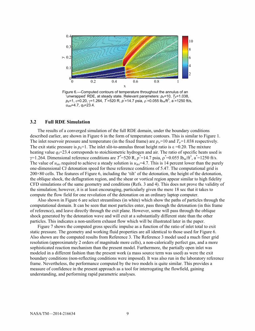
Figure 6.—Computed contours of temperature throughout the annulus of an

‘unwrapped’ RDE, at steady state. Relevant parameters: ptr=10, Ttr=1.038, pb=1, �=0.20, �=1.264, T*=520 R, p*=14.7 psia, �*=0.055 lbm/ft3, a*=1250 ft/s, udet=4.7, q0=23.4.

3.2 Full RDE Simulation

The results of a converged simulation of the full RDE domain, under the boundary conditions described earlier, are shown in Figure 6 in the form of temperature contours. This is similar to Figure 1. The inlet reservoir pressure and temperature (in the fixed frame) are ptr=10 and Ttr=1.038 respectively. The exit static pressure is pb=1. The inlet slit-to-annulus throat height ratio is � =0.20. The mixture heating value q0=23.4 corresponds to stoichiometric hydrogen and air. The ratio of specific heats used is �=1.264. Dimensional reference conditions are T*=520 R, p*=14.7 psia, �*=0.055 lbm/ft3, a*=1250 ft/s. The value of udet required to achieve a steady solution is udet=4.7. This is 14 percent lower than the purely one-dimensional CJ detonation speed for these reference conditions of 5.47. The computational grid is 200×80 cells. The features of Figure 6, including the ‘tilt’ of the detonation, the height of the detonation, the oblique shock, the deflagration region, and the shear or vortical region appear similar to high fidelity CFD simulations of the same geometry and conditions (Refs. 3 and 4). This does not prove the validity of the simulation; however, it is at least encouraging, particularly given the mere 18 sec that it takes to compute the flow field for one revolution of the detonation on an ordinary laptop computer.

Also shown in Figure 6 are select streamlines (in white) which show the paths of particles through the computational domain. It can be seen that most particles enter, pass through the detonation (in this frame of reference), and leave directly through the exit plane. However, some will pass through the oblique shock generated by the detonation wave and will exit at a substantially different state than the other particles. This indicates a non-uniform exhaust flow which will be illustrated later in the paper.

Figure 7 shows the computed gross specific impulse as a function of the ratio of inlet total to exit static pressure. The geometry and working fluid properties are all identical to those used for Figure 6. Also shown are the computed results from Reference 3. The Reference 3 model used a much finer grid resolution (approximately 2 orders of magnitude more cells), a non-calorically perfect gas, and a more sophisticated reaction mechanism than the present model. Furthermore, the partially open inlet was modeled in a different fashion than the present work (a mass source term was used) as were the exit boundary conditions (non-reflecting conditions were imposed). It was also run in the laboratory reference frame. Nevertheless, the performance computed by the two models is quite similar. This provides a measure of confidence in the present approach as a tool for interrogating the flowfield, gaining understanding, and performing rapid parametric analyses.

x

y

0 0.2 0.4 0.6 0.8 10

0.1

0.2

0.3

0.4

2

4

6

8

10

NASA/TM—2014-216634 10

4.0 Discussion 4.1 Semi-Idealized Behavior

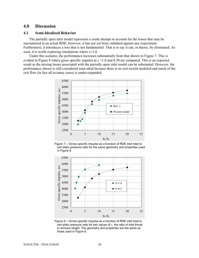
The partially open inlet model represents a crude attempt to account for the losses that may be encountered in an actual RDE; however, it has not yet been validated against any experiment. Furthermore, it introduces a loss that is not fundamental. That is to say it can, in theory, be eliminated. As such, it is worth exploring simulations where �=1.0.

Under this scenario, the performance increases substantially from that shown in Figure 7. This is evident in Figure 8 where gross specific impulse at � =1.0 and 0.20 are compared. This is an expected result as the mixing losses associated with the partially open inlet model can be substantial. However, the performance shown is still considered semi-ideal because there is no exit nozzle modeled and much of the exit flow (in fact all in many cases) is under-expanded.

Figure 7.—Gross specific impulse as a function of RDE inlet total to

exit static pressure ratio for the same geometry and properties used in Figure 6.

Figure 8.—Gross specific impulse as a function of RDE inlet total to

exit static pressure ratio for two values of �, the ratio of inlet throat to annulus height. The geometry and properties are the same as those used in Figure 6.

2500

3000

3500

4000

4500

5000

5500

6000

6500

0 5 10 15 20 25

Gro

ss sp

ecifi

c im

puls

e, s

ec.

ptr/pb

Ref. 3

Present model

2500

3000

3500

4000

4500

5000

5500

6000

6500

0 5 10 15 20 25

Gro

ss sp

ecifi

c im

puls

e, s

ec.

ptr/pb

e=1.0

e=0.2

�

�

NASA/TM—2014-216634 11

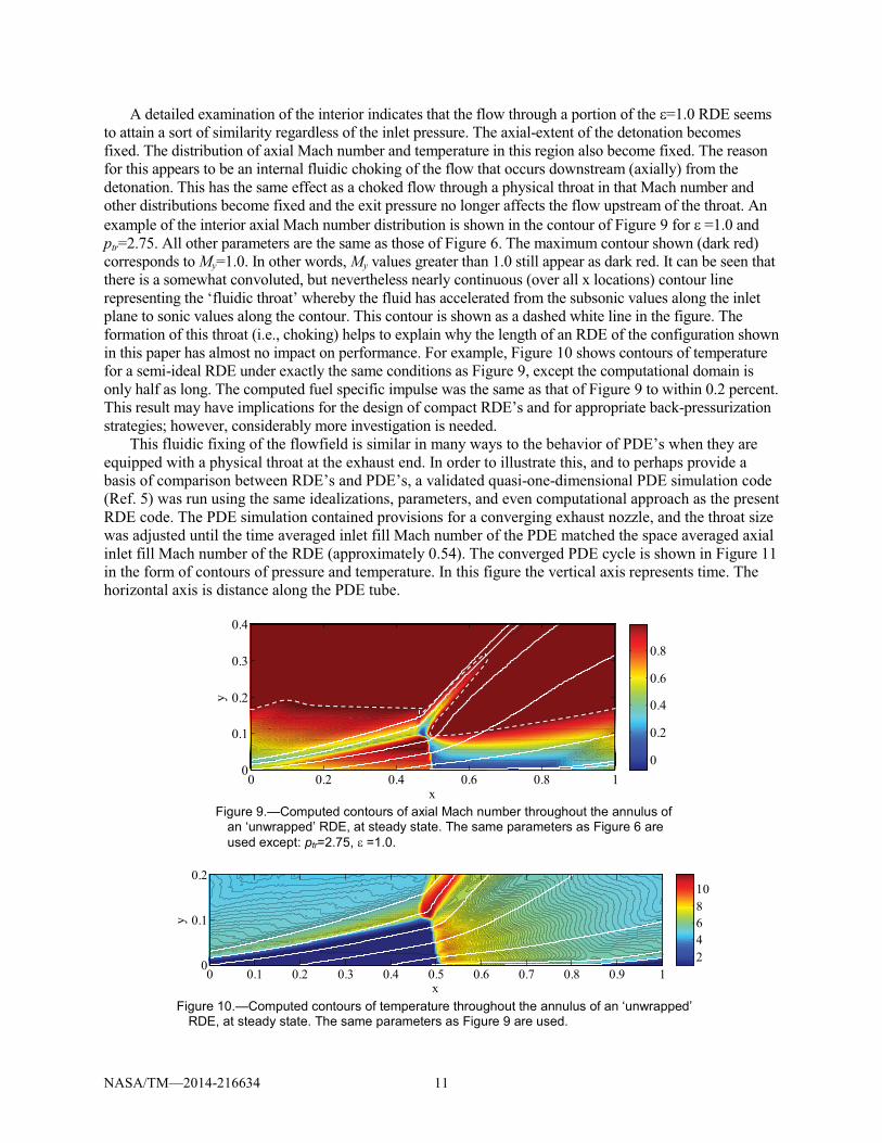
A detailed examination of the interior indicates that the flow through a portion of the �=1.0 RDE seems to attain a sort of similarity regardless of the inlet pressure. The axial-extent of the detonation becomes fixed. The distribution of axial Mach number and temperature in this region also become fixed. The reason for this appears to be an internal fluidic choking of the flow that occurs downstream (axially) from the detonation. This has the same effect as a choked flow through a physical throat in that Mach number and other distributions become fixed and the exit pressure no longer affects the flow upstream of the throat. An example of the interior axial Mach number distribution is shown in the contour of Figure 9 for � =1.0 and ptr=2.75. All other parameters are the same as those of Figure 6. The maximum contour shown (dark red) corresponds to My=1.0. In other words, My values greater than 1.0 still appear as dark red. It can be seen that there is a somewhat convoluted, but nevertheless nearly continuous (over all x locations) contour line representing the ‘fluidic throat’ whereby the fluid has accelerated from the subsonic values along the inlet plane to sonic values along the contour. This contour is shown as a dashed white line in the figure. The formation of this throat (i.e., choking) helps to explain why the length of an RDE of the configuration shown in this paper has almost no impact on performance. For example, Figure 10 shows contours of temperature for a semi-ideal RDE under exactly the same conditions as Figure 9, except the computational domain is only half as long. The computed fuel specific impulse was the same as that of Figure 9 to within 0.2 percent. This result may have implications for the design of compact RDE’s and for appropriate back-pressurization strategies; however, considerably more investigation is needed.

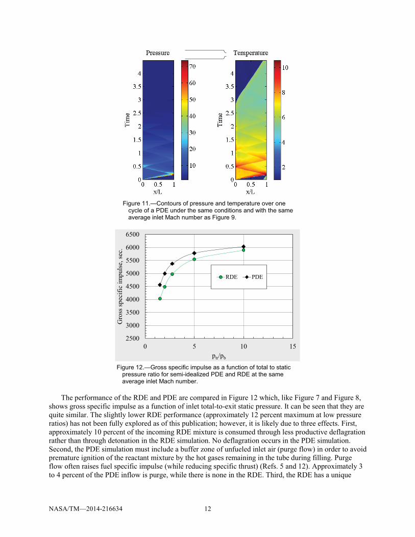
This fluidic fixing of the flowfield is similar in many ways to the behavior of PDE’s when they are equipped with a physical throat at the exhaust end. In order to illustrate this, and to perhaps provide a basis of comparison between RDE’s and PDE’s, a validated quasi-one-dimensional PDE simulation code (Ref. 5) was run using the same idealizations, parameters, and even computational approach as the present RDE code. The PDE simulation contained provisions for a converging exhaust nozzle, and the throat size was adjusted until the time averaged inlet fill Mach number of the PDE matched the space averaged axial inlet fill Mach number of the RDE (approximately 0.54). The converged PDE cycle is shown in Figure 11 in the form of contours of pressure and temperature. In this figure the vertical axis represents time. The horizontal axis is distance along the PDE tube.

Figure 9.—Computed contours of axial Mach number throughout the annulus of

an ‘unwrapped’ RDE, at steady state. The same parameters as Figure 6 are used except: ptr=2.75, � =1.0.

Figure 10.—Computed contours of temperature throughout the annulus of an ‘unwrapped’

RDE, at steady state. The same parameters as Figure 9 are used.

x

y

0 0.2 0.4 0.6 0.8 10

0.1

0.2

0.3

0.4

0

0.2

0.4

0.6

0.8

x

y

0 0.1 0.2 0.3 0.4 0.5 0.6 0.7 0.8 0.9 10

0.1

0.2

246810

NASA/TM—2014-216634 12

Figure 11.—Contours of pressure and temperature over one

cycle of a PDE under the same conditions and with the same average inlet Mach number as Figure 9.

Figure 12.—Gross specific impulse as a function of total to static

pressure ratio for semi-idealized PDE and RDE at the same average inlet Mach number.

The performance of the RDE and PDE are compared in Figure 12 which, like Figure 7 and Figure 8,

shows gross specific impulse as a function of inlet total-to-exit static pressure. It can be seen that they are quite similar. The slightly lower RDE performance (approximately 12 percent maximum at low pressure ratios) has not been fully explored as of this publication; however, it is likely due to three effects. First, approximately 10 percent of the incoming RDE mixture is consumed through less productive deflagration rather than through detonation in the RDE simulation. No deflagration occurs in the PDE simulation. Second, the PDE simulation must include a buffer zone of unfueled inlet air (purge flow) in order to avoid premature ignition of the reactant mixture by the hot gases remaining in the tube during filling. Purge flow often raises fuel specific impulse (while reducing specific thrust) (Refs. 5 and 12). Approximately 3 to 4 percent of the PDE inflow is purge, while there is none in the RDE. Third, the RDE has a unique

2500

3000

3500

4000

4500

5000

5500

6000

6500

0 5 10 15

Gro

ss sp

ecifi

c im

puls

e, s

ec.

ptr/pb

RDE PDE

NASA/TM—2014-216634 13

circumferential velocity element that does not contribute to thrust, but does consume chemical energy. This will be discussed in the next section.

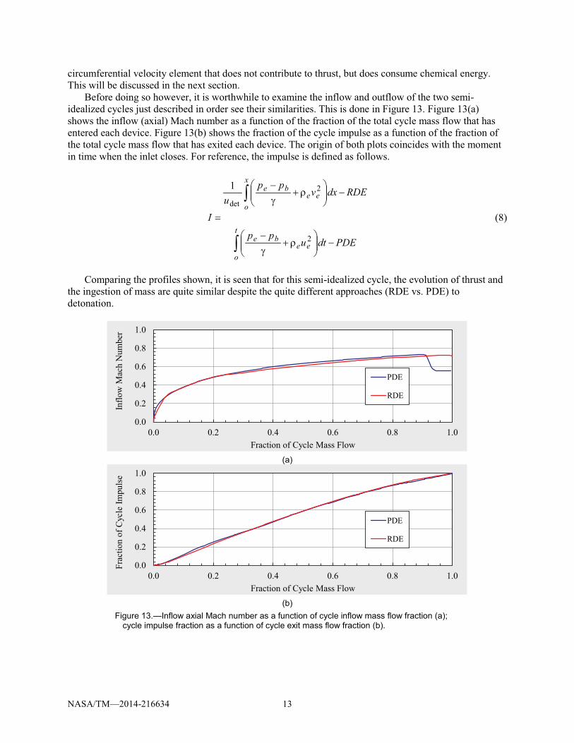
Before doing so however, it is worthwhile to examine the inflow and outflow of the two semi-idealized cycles just described in order see their similarities. This is done in Figure 13. Figure 13(a) shows the inflow (axial) Mach number as a function of the fraction of the total cycle mass flow that has entered each device. Figure 13(b) shows the fraction of the cycle impulse as a function of the fraction of the total cycle mass flow that has exited each device. The origin of both plots coincides with the moment in time when the inlet closes. For reference, the impulse is defined as follows.

PDEdtupp

RDEdxvpp

uI

t

oee

be

x

oee

be

��

��

��

��

��

��

��

��

�

2

2

det

1

(8)

Comparing the profiles shown, it is seen that for this semi-idealized cycle, the evolution of thrust and the ingestion of mass are quite similar despite the quite different approaches (RDE vs. PDE) to detonation.

(a)

(b)

Figure 13.—Inflow axial Mach number as a function of cycle inflow mass flow fraction (a); cycle impulse fraction as a function of cycle exit mass flow fraction (b).

0.0

0.2

0.4

0.6

0.8

1.0

0.0 0.2 0.4 0.6 0.8 1.0

Inflo

w M

ach

Num

ber

Fraction of Cycle Mass Flow

PDE

RDE

0.0

0.2

0.4

0.6

0.8

1.0

0.0 0.2 0.4 0.6 0.8 1.0

Frac

tion

of C

ycle

Impu

lse

Fraction of Cycle Mass Flow

PDE

RDE

NASA/TM—2014-216634 14

4.2 Swirl

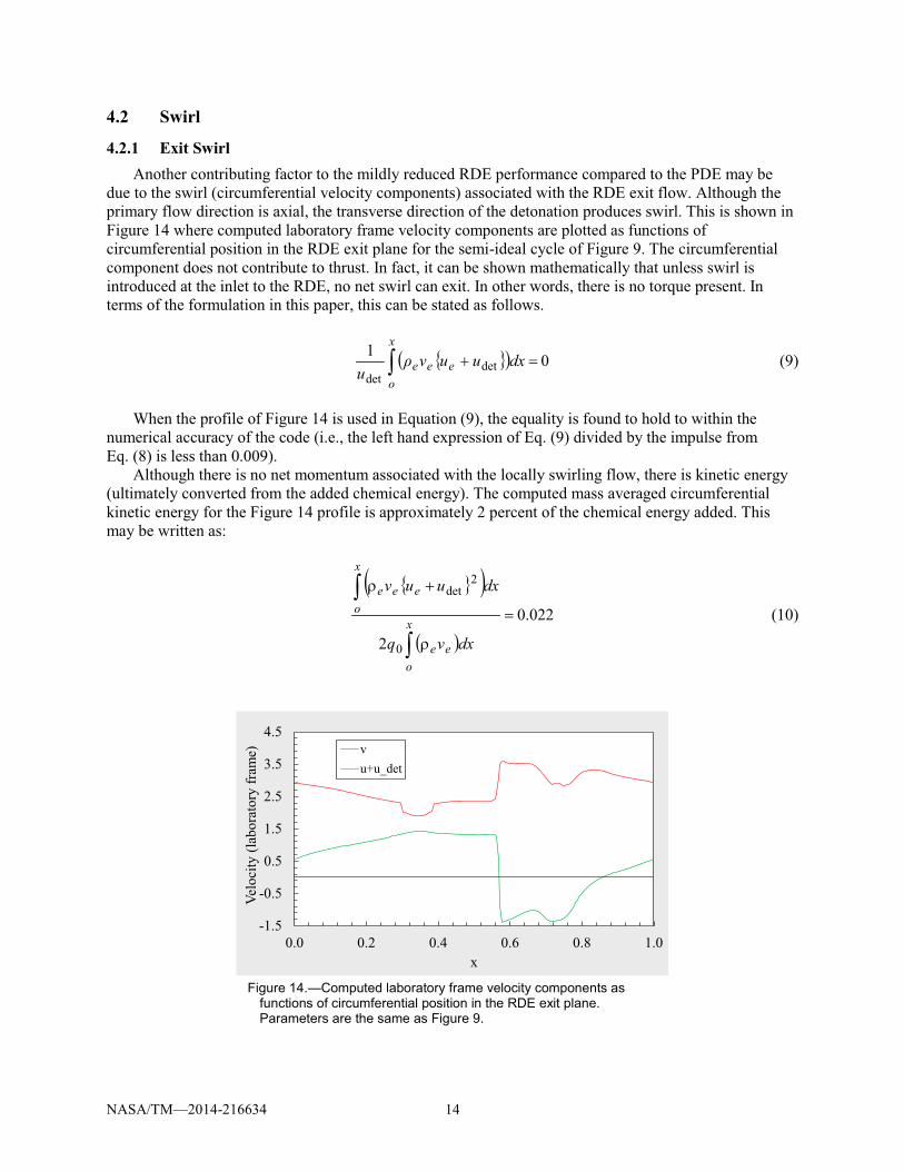
4.2.1 Exit Swirl Another contributing factor to the mildly reduced RDE performance compared to the PDE may be

due to the swirl (circumferential velocity components) associated with the RDE exit flow. Although the primary flow direction is axial, the transverse direction of the detonation produces swirl. This is shown in Figure 14 where computed laboratory frame velocity components are plotted as functions of circumferential position in the RDE exit plane for the semi-ideal cycle of Figure 9. The circumferential component does not contribute to thrust. In fact, it can be shown mathematically that unless swirl is introduced at the inlet to the RDE, no net swirl can exit. In other words, there is no torque present. In terms of the formulation in this paper, this can be stated as follows.

! "� � 01det

det��

x

oeee dxuuv�

u (9)

When the profile of Figure 14 is used in Equation (9), the equality is found to hold to within the numerical accuracy of the code (i.e., the left hand expression of Eq. (9) divided by the impulse from Eq. (8) is less than 0.009).

Although there is no net momentum associated with the locally swirling flow, there is kinetic energy (ultimately converted from the added chemical energy). The computed mass averaged circumferential kinetic energy for the Figure 14 profile is approximately 2 percent of the chemical energy added. This may be written as:

! "� �

� �022.0

2 0

2det

�

�

��

x

oee

x

oeee

dxvq

dxuuv

(10)

Figure 14.—Computed laboratory frame velocity components as

functions of circumferential position in the RDE exit plane. Parameters are the same as Figure 9.

-1.5

-0.5

0.5

1.5

2.5

3.5

4.5

0.0 0.2 0.4 0.6 0.8 1.0

Velo

city

(lab

orat

ory

fram

e)

x

vu+u_det

NASA/TM—2014-216634 15

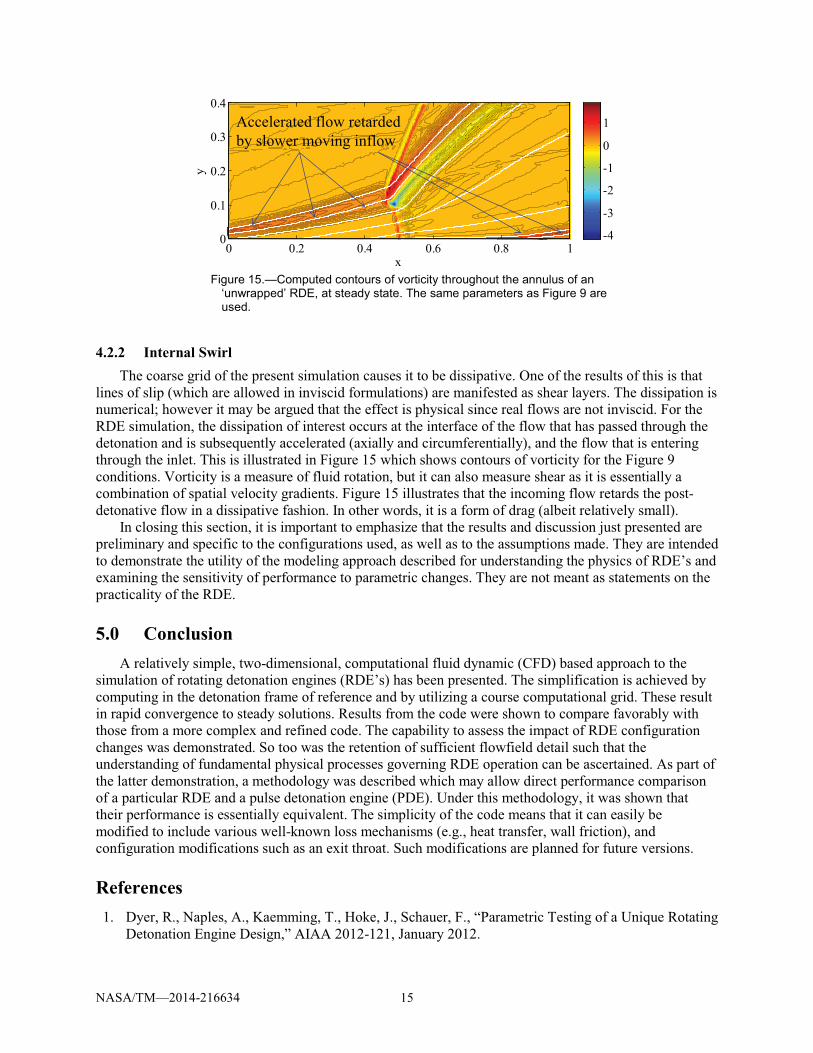
Figure 15.—Computed contours of vorticity throughout the annulus of an

‘unwrapped’ RDE, at steady state. The same parameters as Figure 9 are used.

4.2.2 Internal Swirl The coarse grid of the present simulation causes it to be dissipative. One of the results of this is that

lines of slip (which are allowed in inviscid formulations) are manifested as shear layers. The dissipation is numerical; however it may be argued that the effect is physical since real flows are not inviscid. For the RDE simulation, the dissipation of interest occurs at the interface of the flow that has passed through the detonation and is subsequently accelerated (axially and circumferentially), and the flow that is entering through the inlet. This is illustrated in Figure 15 which shows contours of vorticity for the Figure 9 conditions. Vorticity is a measure of fluid rotation, but it can also measure shear as it is essentially a combination of spatial velocity gradients. Figure 15 illustrates that the incoming flow retards the post-detonative flow in a dissipative fashion. In other words, it is a form of drag (albeit relatively small).

In closing this section, it is important to emphasize that the results and discussion just presented are preliminary and specific to the configurations used, as well as to the assumptions made. They are intended to demonstrate the utility of the modeling approach described for understanding the physics of RDE’s and examining the sensitivity of performance to parametric changes. They are not meant as statements on the practicality of the RDE.

5.0 Conclusion A relatively simple, two-dimensional, computational fluid dynamic (CFD) based approach to the

simulation of rotating detonation engines (RDE’s) has been presented. The simplification is achieved by computing in the detonation frame of reference and by utilizing a course computational grid. These result in rapid convergence to steady solutions. Results from the code were shown to compare favorably with those from a more complex and refined code. The capability to assess the impact of RDE configuration changes was demonstrated. So too was the retention of sufficient flowfield detail such that the understanding of fundamental physical processes governing RDE operation can be ascertained. As part of the latter demonstration, a methodology was described which may allow direct performance comparison of a particular RDE and a pulse detonation engine (PDE). Under this methodology, it was shown that their performance is essentially equivalent. The simplicity of the code means that it can easily be modified to include various well-known loss mechanisms (e.g., heat transfer, wall friction), and configuration modifications such as an exit throat. Such modifications are planned for future versions.

References 1. Dyer, R., Naples, A., Kaemming, T., Hoke, J., Schauer, F., “Parametric Testing of a Unique Rotating

Detonation Engine Design,” AIAA 2012-121, January 2012.

x

y

0 0.2 0.4 0.6 0.8 10

0.1

0.2

0.3

0.4

-4

-3

-2

-1

0

1Accelerated flow retarded by slower moving inflow

NASA/TM—2014-216634 16

2. Naples, Hoke, J., Karnesky, J., Schauer, F., “Flowfield Characterization of a Rotating Detonation Engine,” AIAA 2013-0278, January 2013.

3. Schwer, D.A., and Kailasanath, K., “Numerical Investigation of Rotating Detonation Engines,” AIAA 2010-6880, July 2010.

4. Schwer, D.A., and Kailasanath, K., “Numerical Study of the Effects of Engine Size on Rotating Detonation Engines,” AIAA 2011-581, January 2011.

5. Paxson, D.E., “Performance Evaluation Method for Ideal Air Breathing Pulse Detonation Engines,” Journal of Propulsion and Power, V. 20, No. 5, pp 945-947, 2004, (Also NASA/TM—2001-211085, July 2001).

6. Paxson, D.E., Brophy, C.M. and Bruening, G.B., “Performance Evaluation of a Pulse Detonation Combustion Based Propulsion System Using Multiple Methods,” JANNAF Journal of Propulsion and Energetics, Vol. 3, No. 1, May 2010, pp. 44-54.

7. Nishikawa, H., Kitamura, K., “Very Simple, Carbuncle-Free, Boundary-Layer-Resolving, Rotated-Hybrid Riemann Solvers,” J. of Computational Physics, V. 227, 2008, pp. 2560-2581.

8. Hirsch, C., Numerical Computation of Internal and External Flows, Vol. 2, Wiley and Sons, NY, 1990, pp. 5493-570.

9. Paxson, D.E., “A General Numerical Model for Wave Rotor Analysis,” NASA TM 105740, 1992. 10. Paxson, D.E., “An Improved Numerical Model for Wave Rotor Design and Analysis,” AIAA-93-

0482, January 1993. 11. Thompson, P. H., Compressible Fluid Dynamics, Department of Mechanical Engineering,

Rensselaer Polytechnic Institute, NY, 1988, pp. 349. 12. Schauer, F., Stutrud, J., Bradley, R., “Detonation Initiation Studies and Performance Results for

Pulsed Detonation Engine Applications” AIAA 2001–1129, January 2001.

Numerical Analysis of a Rotating Detonation Engine in … E. Paxson Glenn Research Center,...

Documents

Transcript of Numerical Analysis of a Rotating Detonation Engine in … E. Paxson Glenn Research Center,...