
NTU IM Page 1 of 35 Modelling Data-Centric Routing in Wireless Sensor Networks IEEE INFOCOM 2002....
35
NTU IM Page 1 of 35 Modelling Data-Centric Routi ng in Wireless Sensor Netwo rks IEEE INFOCOM 2002. Author: Bhaskar Krishnamachari Deborah Estrin Stephen Wicker Presented by: 高高高 (R91725061)
-
Upload
kellie-ford -
Category
Documents
-
view
216 -
download
3
Transcript of NTU IM Page 1 of 35 Modelling Data-Centric Routing in Wireless Sensor Networks IEEE INFOCOM 2002....

NTU IM Page 1 of 35
Modelling Data-Centric Routing in Wireless Sensor Networks
IEEE INFOCOM 2002.Author:Bhaskar KrishnamachariDeborah EstrinStephen Wicker
Presented by:高柏鈞 (R91725061)

NTU IM Page 2 of 35
Outline
IntroductionRouting ModelsData AggregationEnergy Savings due to Data AggregationDelay due to Data AggregationRobustness due to Data AggregationShortcomings of the ModellingConclusions

NTU IM Page 3 of 35
Introduction
The Wireless Sensor Networks features: Consist many inexpensive wireless
nodes. Each node with some computational
power and sensing capability. Operating in an unattended mode.
Because of miniature sensing and radio capability, there are many research with further improvements in cost and capabilities.

NTU IM Page 4 of 35
Introduction (Cont’d)
Similar to mobile ad-hoc networks (MANETs) Both involve multi-hop communications.
Significantly different for sensor networks From multiple data sources to a data sink (l
ike reverse-multicast) rather than pairs. Base on common phenomena, there is likel
y to be some redundancy data. In most scenarios the sensors are not mobi
le.

NTU IM Page 5 of 35
Introduction (Cont’d)
The single major resource constraint in sensor network is that of Energy.
The energy problem is much worse than MANETs, because of unattended operation environment.
Manage Energy Resources more carefully- Precludes high data rate communication.
End-to-end routing protocols that have been proposed for MANETs are not suitable.

NTU IM Page 6 of 35
Introduction (Cont’d)
Data Aggregation has been put forward as a useful paradigm for sensor networks routing.
Eliminating Redundancy Minimizing the number of transmissions Saving Energy
In this paper, we compare the gains and tradeoffs by using two routing models.

NTU IM Page 7 of 35
Routing Models
Two Routing Models:1. Address-centric Protocol (AC): Not use
data aggregation, each source independently sends data along the shortest path.
2. Data-centric Protocol (DC): Use data aggregation, regards as data content and perform aggregation function on intermediate.

NTU IM Page 8 of 35
Routing Models (Cont’d)

NTU IM Page 9 of 35
Routing Models (Cont’d)
Differentiating Scenarios1. All sources send completely different
information (no redundancy).2. All sources send identical information
(complete redundancy).3. The sources send information with
some intermediate level of redundancy.

NTU IM Page 10 of 35
Routing Models (Cont’d)
In case 1, both AC and DC protocols will incur the same number of transmissions.
In case 2, the AC protocol can be modified better than the DC protocol.
Let sink monitor the incoming information, if duplication happen then ask others to stop transmitting.
In case 3, the AC protocol cannot be modified much better than the DC, so in this paper we assume this scenario holds.

NTU IM Page 11 of 35
Data Aggregation
Optimal Aggregation k sources, labelled S1 through Sk. A sink, labelled D. Network Graph G=(V,E) consist of all nodes V,
with E consisting of edges between nodes that can communicate with each other directly.
With the Assumption of the number of transmissions from any node in the data aggregation tree is exactly one, the tree can be thought of as the reverse of a multicast tree: all the sources are sending a single packet to the same receiver.

NTU IM Page 12 of 35
Data Aggregation (Cont’d)
Result 1: it is well-known the multicast tree with a minimum number of edges is a minimum Steiner tree, so the optimum number of transmissions required per datum for the DC protocol is equal to the number of edges in the minimum Steiner tree which contains the node set (S1,…Sk, D).
Corollary: Assuming an arbitrary placement of sources, the task of doing DC routing with optimal data aggregation is NP-hard.

NTU IM Page 13 of 35
Data Aggregation (Cont’d)
Minimum Steiner tree

NTU IM Page 14 of 35
Data Aggregation (Cont’d)
Suboptimal Aggregation1. Center at Nearest Source (CNS): the source
nearest the sink acts as aggregation point.2. Shortest Paths Tree (SPT): Combine all shor
test paths from all sources to the sink.3. Greedy incremental Tree (GIT): Each step co
nnect the source closest to the current tree.These heuristics of the data aggregation are NP-complete, prove by reference
[11] M.R. Garey and D.S. Johnson, Computers and Intractability: A Guide to the Theory of NP-completeness, 1979.

NTU IM Page 15 of 35
Data Aggregation (Cont’d)
Performance measures Energy Savings: due to aggregation the
information, the number of transmissions is reduced, translating to a savings in energy.
Delay: data from nearer sources may have to be held back in order to wait for farther information to combine.
Robustness: with data aggregation there is a decrease in the marginal energy cost of connecting additional sources to the sink.

NTU IM Page 16 of 35
Data Aggregation (Cont’d)
Source Placement Models Event-Radius Model (ER)
1. S is sensing range for event
2. The average number of sources is about π* S2 * n , where n is total nodes of this square.

NTU IM Page 17 of 35
Data Aggregation (Cont’d)
Source Placement Models (Cont’d) Random-Sources Model (RS)
1. k of the nodes that are not sinks are randomly selected to be sources.
2. The sources are not necessarily clustered near each other.

NTU IM Page 18 of 35
Energy Savings
Theoretical Results Give some analytical bounds on the
energy costs and savings based on:1. The distances between the sources and
the sink.2. The inter-distances among the sources.
Upshot: greatest gains when 1. The sources are all close together.2. The sources are far away from the sink.

NTU IM Page 19 of 35
Energy Savings (Cont’d)
Let di be the distance of the shortest path from source Si to the sink in the graph.
Per datum, the total number of transmissions required for the optimal AC protocol (NA) is:
Result 2: Let the number of transmissions required for the optimal DC protocol be ND. Then ND ≤ NA.
NA = d1 + d2 + … + dk = sum(di) (1)

NTU IM Page 20 of 35
Energy Savings (Cont’d)
Def: The diameter X = maxi,j∈SourcesSP(i, j) , where SP(i, j) is the shortest number of hops needed to go from node i to j in graph.
Result 3: if source S1 to Sk have a diameter X ≥ 1, then the following bounds hold:
ND ≤ (k-1)X + min(di) (2)
ND ≥ (k-1)*1 + min(di) (3)

NTU IM Page 21 of 35
Energy Savings (Cont’d)
Result 4: if X < min(di), then ND < NA.
Base on the (2)
ND < (k-1)X + min(di) < k * min(di)
ND < sum(di) = NA (4)
Def: the fractional savings (FS),
FS = (NA - ND) / (NA) = 1 – ND / NA (5) FS can range from 0 (no savings) to 1 (100% savings)

NTU IM Page 22 of 35
Energy Savings (Cont’d)
Result 5: directly from (2) and (3), FS satisfies the following bounds:
FS ≥ 1-((k-1)X + min(di)) / sum(di) (6)
FS ≤ 1-(min(di) + k -1 ) / sum(di) (7)
ND ≤ (k-1)X + min(di) (2)
ND ≥ (k-1)*1 + min(di) (3)

NTU IM Page 23 of 35
Energy Savings (Cont’d)
Assume that all sources are at the same shortest-path distance from the sink, i.e. min(di) = max(di) = d. Then we have that
Result 6: Assume X and k are fixed, then

NTU IM Page 24 of 35
Energy Savings (Cont’d)
Proof,

NTU IM Page 25 of 35
Energy Savings (Cont’d)
Result 7: if the subgraph G’ of the communication graph G induced by the set of source nodes (S1,…Sk) is connected, the optimal data aggregation tree can be formed in polynomial time.
Result 8: in the ER model, when R>2S, the optimal data aggregation tree can be formed in polynomial time.

NTU IM Page 26 of 35
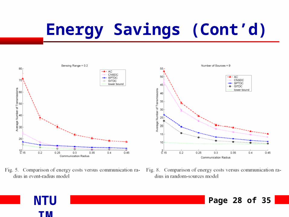
Energy Savings (Cont’d)
Experimental Results For the ER model, sensing range S from
0.10, 0.15, 0.20, 0.25, 0.30 are tested. For the RS model, the number of sources k
is varied 1 to 15 in increments of 2. For both, the communication radius R is
varied from 0.15 to 0.45 in increments of 0.05.
For each combination of S or k and R 100 experiments were run.

NTU IM Page 27 of 35
Energy Savings (Cont’d)
NTU IM Page 28 of 35
Energy Savings (Cont’d)

NTU IM Page 29 of 35
Energy Savings (Cont’d)

NTU IM Page 30 of 35
Delay

NTU IM Page 31 of 35
Delay (Cont’d)

NTU IM Page 32 of 35
Robustness

NTU IM Page 33 of 35
Shortcomings
1. Make a stark contrast between routing protocols, AC versus DC, is overly simplistic.
2. Lack of considering overhead costs involved in setting up or maintaining the routing paths.
3. The analysis of the delay focused only on the latency due to aggregation.
4. The analysis has focused on the case where there is a single sink.

NTU IM Page 34 of 35
Conclusions
Whether the sources are clustered near each other (ER) or located randomly (RS), significant energy gains are possible with data aggregation.
These gains are greatest when The number of sources (k) is large . The sources are located relatively close
to each other. The sources are far from the sink.

NTU IM Page 35 of 35
Conclusions (Cont’d)
The modelling suggest that aggregation latency could be non-negligible and should be taken into consideration during the design process.


![Curso de Aperturas Abiertas. Panov & Estrin [63]](https://static.fdocument.pub/doc/165x107/577cdbb11a28ab9e78a8d1db/curso-de-aperturas-abiertas-panov-estrin-63.jpg)
