Non-Markovian quantum jump with generalized Lindblad master equation

X. L. Huang (黄晓理�,* H. Y. Sun (孙慧颖�, and X. X. Yi (衣学喜�†

School of Physics and Optoelectronic Technology, Dalian University of Technology, Dalian 116024, China�Received 27 June 2008; revised manuscript received 8 September 2008; published 6 October 2008�

The Monte Carlo wave function method or the quantum-trajectory–jump approach is a powerful tool tostudy dissipative dynamics governed by the Markovian master equation, in particular for high-dimensionalsystems and when it is difficult to simulate directly. We extend this method to the non-Markovian casedescribed by the generalized Lindblad master equation. Two examples to illustrate the method are presentedand discussed. The results show that the method can correctly reproduce the dissipative dynamics for thesystem. The difference between this method and the traditional Markovian jump approach and the computa-tional efficiency of this method is also discussed.

DOI: 10.1103/PhysRevE.78.041107 PACS number�s�: 05.60.Gg, 03.65.Yz, 42.50.Lc

I. INTRODUCTION

Since the pioneering work of Albert Einstein, who ex-plained the phenomenon of dissipation and Brownian motionin his annus mirabilis of 1905 by use of statistical methods,a rich variety of methods to tackle quantum fluctuations andquantum dissipation in open systems has been proposed�1,2�. Among them, the quantum master equation �QME� ap-proach and the quantum Langevin description �QLE� �3� aretwo powerful functional integral techniques for the study ofthe time evolution of open quantum systems. The quantummaster equation can be divided into two categories: Markov-ian and non-Markovian. The Markovian master equation �4��especially in the Lindbald form� can be derived with theweak-coupling limit �or the Born approximation� and theMarkovian approximation. It can be solved analytically �5�for some special cases, but for most cases we have to solveand simulate it numerically by the Monte Carlo wave func-tion method or quantum-trajectory–jump approach �6–11�.This method is very effective for qubit systems even with alarge number of qubits—say, n=24 �9�.

However, the dynamics of an open system is not alwaysMarkovian. Strong system-environment couplings, correla-tion and entanglement in the initial state, and structured res-ervoirs may lead the dynamics far from Markovian. Manymethods have been proposed to describe the non-Markovianprocess, including the Lindblad equation with time-dependent decay rates �12�, generalized Lindblad equation�13� obtained from the correlated projection superoperatortechniques �14,15�, phenomenological memory kernel masterequation �16,17�, and the post-Markovian master equation�18–20�. The first two methods are local in time, while thelast two involve an integral of time. For the first method, theonly difference from the Markovian master equation is thatthe decay rates in the equation are time dependent. Thesedecay rates may take not only positive values, but also nega-tive ones. When decay rates are positive, the MarkovianMonte Carlo wave function method can directly be used.However, the method is not available when the decay rates

are negative. This problem was solved in Ref. �21� by intro-ducing reversed jumps.

The generalized Lindblad master equation can well de-scribe the dynamics of an open system beyond the Markov-ian limit; especially, it is very effective for an environmentcomposed of spins �22–24� and structured reservoirs �25�.However, the extension of the Monte Carlo simulation to thisequation remains untouched. In this paper, we will explorethe unraveling and quantum trajectory approach for the gen-eralized Lindblad equation. The structure of this paper isorganized as follows. In Sec. II we briefly review the gener-alized Lindblad equation. In Sec. III we give the unravelingof this equation and generalize the Monte Carlo method tothis equation. Two examples are presented in Sec. IV. Fi-nally, we conclude our results in Sec. V.

II. GENERALIZED LINDBLAD MASTER EQUATION

The equation that governs the dynamics of an open quan-tum system can be derived by means of the projection super-operator technique �12,14�. The form �Markovian or non-Markovian� of the master equation crucially depends on theapproximation used in the derivation, reflected in the projec-tion superoperator chosen. When we project the total systemstate onto a tensor product, we can obtain the Markovianmaster equation, whereas a non-Markovian master equationcan be obtained when we use a correlated projection. Thefollowing is the master equation derived by this method, andit is called the generalized Lindblad master equation �13�:

d

dt�m = − i�Hm,�m� + �

n�

�Rmn� �nRmn

�† −1

2�Rnm

�† Rnm� ,�m� ,

�1�

where Hm are Hermitian operators and Rmn� are arbitrary sys-

tem operators depending on the form of system-environmentinteractions. If we have only a single component �S=�1, thisequation obviously reduces to the ordinary Markovian mas-ter equation. In this paper we will focus on the case wherewe have at least two components. The state of the reducedsystem in this case is �S=�m�m; we recall that Tr �m�1.

*ghost820521@163.com†yixx@dlut.edu.cn

PHYSICAL REVIEW E 78, 041107 �2008�

1539-3755/2008/78�4�/041107�5� ©2008 The American Physical Society041107-1

III. QUANTUM JUMP

For clarity, we define the jump operators Wmn� =Rmn

� andnonjump operators Wmm

0 =1− iHmdt, where the non-Hermitian effective Hamiltonian is given by Hm=Hm

− 12 i�n�Rnm

�† Rnm� . There are two subscripts and one superscript

for the operator Wmn� . The first subscript m denotes the index

of the component corresponding to �m, while the second sub-script n denotes the index of the component for the operationacted on; the superscript � represents the jump mode. Ini-tially we assume that each operator �m�t0� can be written as�m�t0�= �m�t0����m�t0�, where �m�t0�� is a non-normalizedwave function. After an infinitesimal time dt, it evolves intothe state

�m�t0 + dt� = �n�

�mn� ���mn

� dpmn� + �mm

0 ���mm0 dpmm

0 , �2�

where the new states are defined by

�mn� � =

pmWmn� �n�t��

�Wmn� �n�t���

�3�

and

�mm0 � =

pmWmm0 �m�t��

�Wmm0 �m�t���

, �4�

with probabilities

dpmn� =

1

pm��n�t0�Wmn

�† Wmn� �n�t0��dt ,

dpmm0 =

1

pm��m�t0�Wmm

0† Wmm0 �m�t0�� , �5�

respectively. In Eqs. �3� and �4�,

pm = �n�

��n�t0�Wmn�† Wmn

� �n�t0��dt + ��m�t0�Wmm0† Wmm

0 �m�t0��

�6�

is the weight for the component �m that satisfies

pm = Tr�m�t + dt� . �7�

Note that the jumps for �m depend on the other components�n �n�m� of the reduced density matrix �. This makes ourmethod different from the traditional quantum jump method.

We can prove this unraveling by putting the jump andnonjump states �3� and �4� and the probabilities �5� and �6�into Eq. �2�,

�m�t + dt� = �n�

Wmn� �n�t����n�t�Wmn

�† dt + Wmm0 �m�t��

���m�t�Wmm0† . �8�

Simple algebra shows that in the limit dt→0, Eq. �8� revealsEq. �1�. The evolution governed by Eq. �1� can be simulatednumerically by the so-called Monte Carlo wave function ap-proach according to the unraveling given above. We start thetime evolution from the state ��t0�=�m�m�t0�=�m�m�t0����m�t0�, where �m �m=1,2 ,3 , . . . � are the com-

ponents for �. At time t0+dt, where dt is much smaller thanthe time scale relevant for the evolution of the density ma-trix, a random number �, which is randomly distributed inthe unit interval �0, 1�, is used to determine the jump. Notethat all the components are controlled by this random num-ber. For each component �m�, if 0���dpm1

1 , it jumps to�m1

1 �, if dpm11 ���dpm1

1 +dpm12 , it jumps to �m1

2 �, and so on.These jumps are all operated on the component �1; if��dpm1

� �����dpm1� +dpm2

1 , it jumps to the component2—namely, �m2

1 �. Jumps to the other components can beestablished in a similar way. If ���n�dpmn

� , a nonjump takesplace and the state ends up in �mm

0 �. This operation is actedon the component �m itself. We define a generalized jumpsuperoperator Wi, which denotes all jumps for all the com-ponents controlled by this random number. We repeat thisprocess as many times as n=t /dt for all components, wheret is the total evolution time. We call this single evolution ageneralized quantum trajectory. This trajectory contains allthe components of the density matrix. Given an operator A,we can write its mean value �A��t�=Tr�A��t�� as an averageover N trajectories as

�A��t� = limN→

�j=1

N

�m

��m,j�t�A�m,j�t�� . �9�

IV. APPLICATION

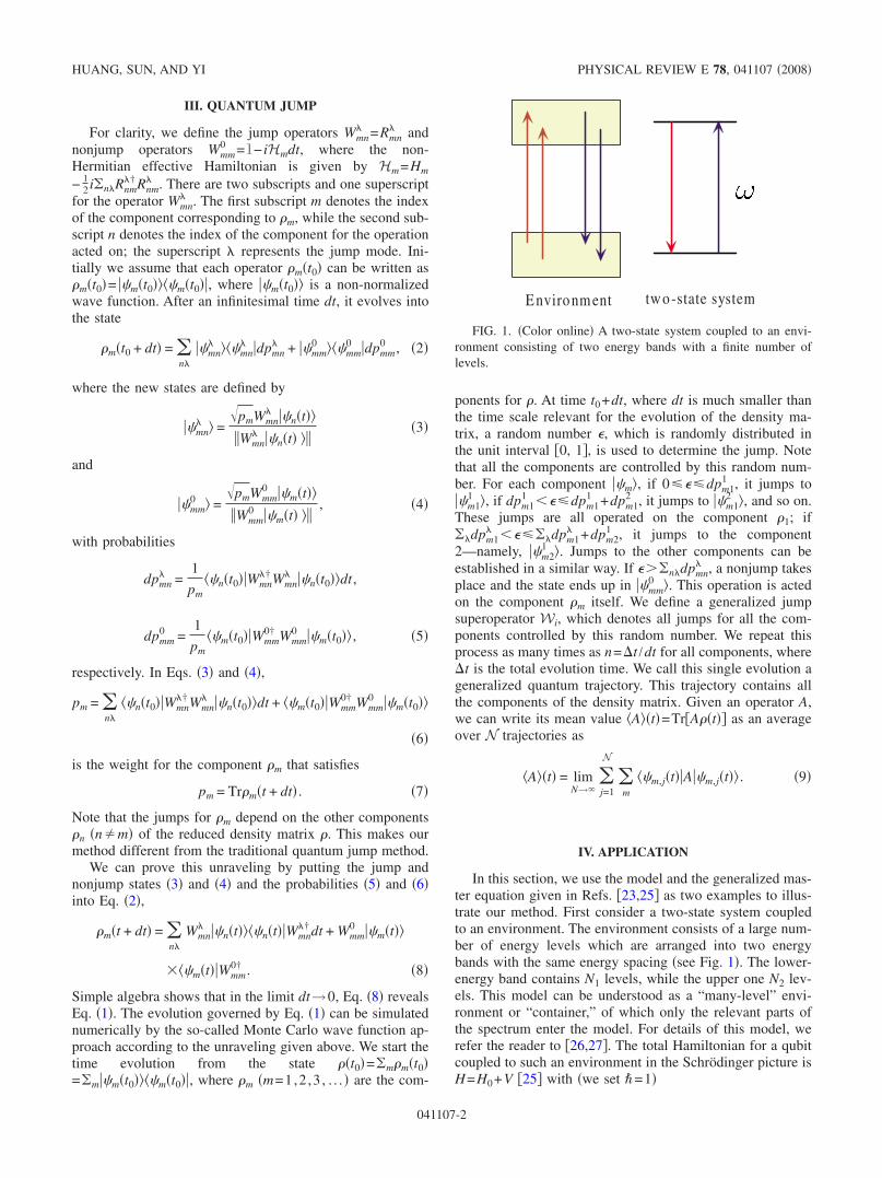
In this section, we use the model and the generalized mas-ter equation given in Refs. �23,25� as two examples to illus-trate our method. First consider a two-state system coupledto an environment. The environment consists of a large num-ber of energy levels which are arranged into two energybands with the same energy spacing �see Fig. 1�. The lower-energy band contains N1 levels, while the upper one N2 lev-els. This model can be understood as a “many-level” envi-ronment or “container,” of which only the relevant parts ofthe spectrum enter the model. For details of this model, werefer the reader to �26,27�. The total Hamiltonian for a qubitcoupled to such an environment in the Schrödinger picture isH=H0+V �25� with �we set �=1�

Environm ent tw o-state system

FIG. 1. �Color online� A two-state system coupled to an envi-ronment consisting of two energy bands with a finite number oflevels.

HUANG, SUN, AND YI PHYSICAL REVIEW E 78, 041107 �2008�

041107-2

H0 =1

2� z + �

n1

��

N1n1n1��n1 + �

n2

�� +��

N2n2n2��n2 ,

V = � �n1n2

c�n1,n2� +n1��n2 + H.c.,

where the index n1 denotes the levels of the lower-energyband and n2 denotes the levels of the upper band, and z and � are Pauli operators. � is the overall strength of the inter-action, and c�n1 ,n2� are coupling constants; they are inde-pendent of each other and are identically distributed, satisfy-ing

�c�n1,n2�� = 0,

�c�n1,n2�c�n1�,n2��� = 0,

�c�n1,n2�c*�n1�,n2��� = �n1,n1��n2,n2�

.

According to H0, one can transform the problem into theinteraction picture and, with the help of the projection super-operator technique, obtain the non-Markovian evolutionequation as

d

dt�S

�1��t� = �1 +�S�2��t� − −

�2

2� + −,�S

�1��t�� ,

d

dt�S

�2��t� = �2 −�S�1��t� + −

�1

2� − +,�S

�2��t�� , �10�

where

�i =2��2Ni

���i = 1,2� .

With the definitions of �1=�n1n1��n1 and �2=�n2

n2��n2,�1+�2=1E, the two non-normalized density matrices can beobtained by �S

�i�=TrE��i�T�, i=1,2, where �T is the total den-sity matrix for the system and environment. The reduceddensity matrix for the system is then given by �=�S

�1�+�S�2�.

We note that in Eq. �10�, there are no environment operatorsother than the two �c-number� parameters �1 and �2. Theinitial state of the environment is taken into account bymeans of the distribution of the initial �S

�1� and �S�2�; its effect

on the system dynamics is plotted in Figs. 2 and 3. Thisequation can be written in the form of Eq. �1� by settingHi=0, R11=R22=0, R12= �1 +, and R21= �2 −. In thismodel, there is only one jump operator for each component,i.e., W12

1 = �1 + and W211 = �2 −, and nonjump operators

Wmm0 =1− iHmdt, with H1=− 1

2�2 + − and H2=− 12�1 − +.

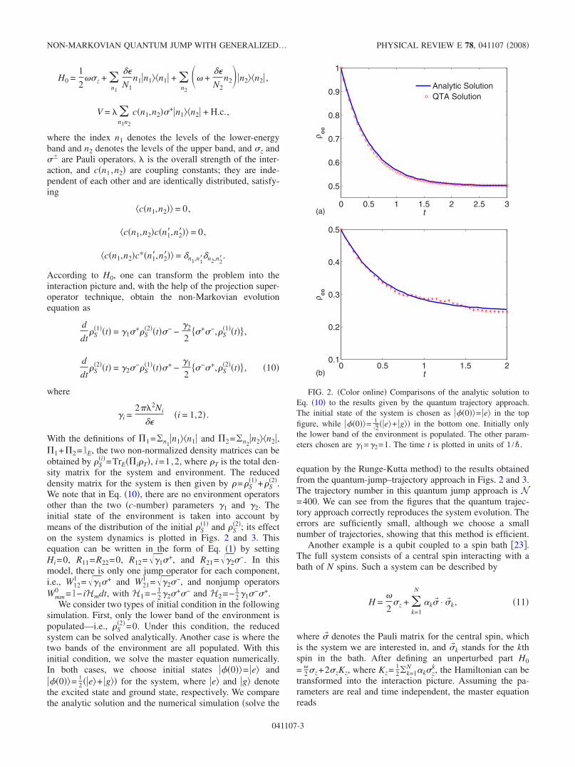
We consider two types of initial condition in the followingsimulation. First, only the lower band of the environment ispopulated—i.e., �S

�2�=0. Under this condition, the reducedsystem can be solved analytically. Another case is where thetwo bands of the environment are all populated. With thisinitial condition, we solve the master equation numerically.In both cases, we choose initial states ��0��= e� and��0��= 1

2 �e�+ g�� for the system, where e� and g� denotethe excited state and ground state, respectively. We comparethe analytic solution and the numerical simulation �solve the

equation by the Runge-Kutta method� to the results obtainedfrom the quantum-jump–trajectory approach in Figs. 2 and 3.The trajectory number in this quantum jump approach is N=400. We can see from the figures that the quantum trajec-tory approach correctly reproduces the system evolution. Theerrors are sufficiently small, although we choose a smallnumber of trajectories, showing that this method is efficient.

Another example is a qubit coupled to a spin bath �23�.The full system consists of a central spin interacting with abath of N spins. Such a system can be described by

H =�

2 z + �

k=1

N

�k � · � k, �11�

where � denotes the Pauli matrix for the central spin, whichis the system we are interested in, and � k stands for the kthspin in the bath. After defining an unperturbed part H0

= �2 z+2 zKz, where Kz= 1

2�k=1N �k z

k, the Hamiltonian can betransformed into the interaction picture. Assuming the pa-rameters are real and time independent, the master equationreads

0 0.5 1 1.5 2 2.5 3

0.5

0.6

0.7

0.8

0.9

1

t

ρ ee

Analytic SolutionQTA Solution

0 0.5 1 1.5 20.1

0.2

0.3

0.4

0.5

t

ρ ee

(b)

(a)

FIG. 2. �Color online� Comparisons of the analytic solution toEq. �10� to the results given by the quantum trajectory approach.The initial state of the system is chosen as ��0��= e� in the topfigure, while ��0��= 1

2�e�+ g�� in the bottom one. Initially only

the lower band of the environment is populated. The other param-eters chosen are �1=�2=1. The time t is plotted in units of 1 /�.

NON-MARKOVIAN QUANTUM JUMP WITH GENERALIZED… PHYSICAL REVIEW E 78, 041107 �2008�

041107-3

d

dt�m = gm+1 +�m+1 − + fm−1 −�m−1 + −

1

2fm� + −,�m�

−1

2gm� − +,�m� , �12�

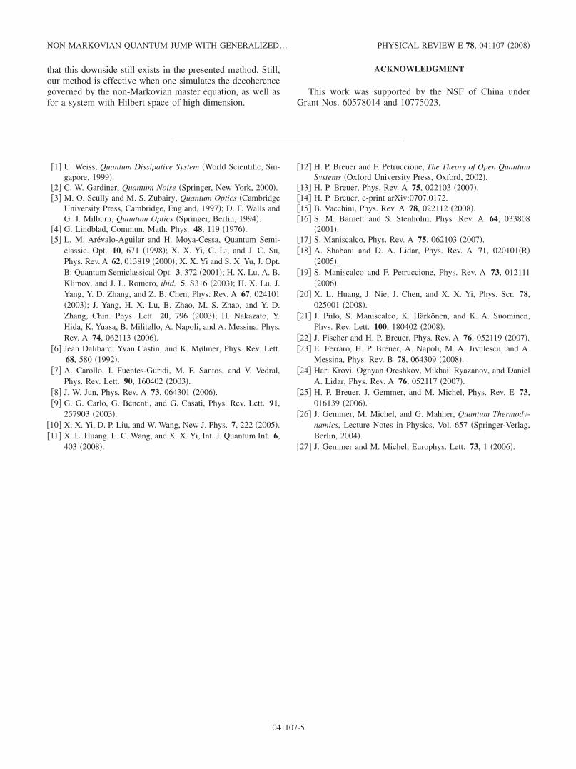
where �m=TrB��T�m�, �T is the density matrix for the totalsystem �the central spin plus the bath�, and �m is a projectionsuperoperator that projects the z component of the bath an-gular momentum into an eigenvector with eigenvalue m. Wetake N=2 as an example; then, the density matrix of thecentral spin has three components, denoted by �1, �0, and�−1, respectively. Each component has two jump operators,which act on the other two components, and a nonjump op-erator, which acts on itself. The comparison between directnumerical simulations �by the Runge-Kutta method� and thequantum trajectory method is shown in Fig. 4. Here the tra-jectory number is chosen to be N=4000. We can find that asthe number of jump operators and components increases, thenumber of quantum trajectories with which we can obtain acorrect result increases.

V. CONCLUSION AND DISCUSSION

In this paper, we have developed an efficient unravelingfor the generalized Lindblad master equation. Based on thisunraveling, a generalized Monte Carlo wave functionmethod is presented. It is worth addressing the fact that inthis Monte Carlo wave function method, we need only tostore M non-normalized wave functions—i.e., M length-Nvectors �M denotes the number of the components for thereduced density matrix and N stands for the dimension of theHilbert space� instead of the density operator, which are MN�N matrices—hence this method saves the computer timeand space. The difference between the ordinary quantumjump method and the present one is that the latter describes anon-Markovian dynamics. In addition, the point that eachcomponent �i of the density matrix is non-normalized andjumps along the component �i depends on a component otherthan �i, which is also different. By successfully simulatingthe coupling among those components, this method cansimulate the non-Markovian dynamics efficiently. Furtherexamination shows that the computational complexity in-creases with the number of the components. The increasedcomplexity due to the increase of the components and jumpoperators can by analyzed as follows. Assume the jump op-erators and the number of jump operators are restricted to bethe same for each component; the possible jump mode for�= ��1 ,�2 , . . . � or the number of generalized jump superop-erators W is

= M�J − 1� + 1. �13�

Here J is the number of jump operators for each component�including the nonjump operator�. The role that plays issimilar to the number of jump operators in the ordinary Mar-kovian master equation. It is well known that one downsideof the quantum jump approach is the complexity growth asthe jump operators proliferate. From Eq. �13�, we can find

0 0.5 1 1.5 20.7

0.75

0.8

0.85

0.9

0.95

1

t

ρ ee

Numerical solutionQTA solution

0 0.5 1 1.5 20.1

0.2

0.3

0.4

0.5

t

ρ eg

(b)

(a)

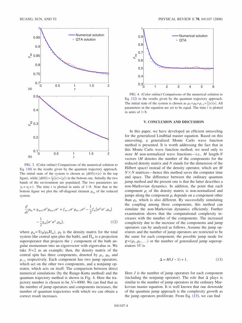
FIG. 3. �Color online� Comparisons of the numerical solution toEq. �10� to the results given by the quantum trajectory approach.The initial state of the system is chosen as ��0��= e� in the topfigure, while ��0��= 1

2�e�+ g�� in the bottom one. Initially the two

bands of the environment are populated. The two parameters are�1=�2=1. The time t is plotted in units of 1 /�. Note that in thebottom figure we plot the off-diagonal element �eg of the reducedsystem.

0 1 2 3 4 5 60.3

0.4

0.5

0.6

0.7

0.8

0.9

1

ρ ee

Numerical solutionQTA

FIG. 4. �Color online� Comparisons of the numerical solution toEq. �12� to the results given by the quantum trajectory approach.The initial state of the system is chosen as �1=�0=�−1= 1

3 e��e. Allparameters in the equation are set to be equal. The time t is plottedin units of 1 /�.

HUANG, SUN, AND YI PHYSICAL REVIEW E 78, 041107 �2008�

041107-4

that this downside still exists in the presented method. Still,our method is effective when one simulates the decoherencegoverned by the non-Markovian master equation, as well asfor a system with Hilbert space of high dimension.

ACKNOWLEDGMENT

This work was supported by the NSF of China underGrant Nos. 60578014 and 10775023.

�1� U. Weiss, Quantum Dissipative System �World Scientific, Sin-gapore, 1999�.

�2� C. W. Gardiner, Quantum Noise �Springer, New York, 2000�.�3� M. O. Scully and M. S. Zubairy, Quantum Optics �Cambridge

University Press, Cambridge, England, 1997�; D. F. Walls andG. J. Milburn, Quantum Optics �Springer, Berlin, 1994�.

�4� G. Lindblad, Commun. Math. Phys. 48, 119 �1976�.�5� L. M. Arévalo-Aguilar and H. Moya-Cessa, Quantum Semi-

classic. Opt. 10, 671 �1998�; X. X. Yi, C. Li, and J. C. Su,Phys. Rev. A 62, 013819 �2000�; X. X. Yi and S. X. Yu, J. Opt.B: Quantum Semiclassical Opt. 3, 372 �2001�; H. X. Lu, A. B.Klimov, and J. L. Romero, ibid. 5, S316 �2003�; H. X. Lu, J.Yang, Y. D. Zhang, and Z. B. Chen, Phys. Rev. A 67, 024101�2003�; J. Yang, H. X. Lu, B. Zhao, M. S. Zhao, and Y. D.Zhang, Chin. Phys. Lett. 20, 796 �2003�; H. Nakazato, Y.Hida, K. Yuasa, B. Militello, A. Napoli, and A. Messina, Phys.Rev. A 74, 062113 �2006�.

�6� Jean Dalibard, Yvan Castin, and K. Mølmer, Phys. Rev. Lett.68, 580 �1992�.

�7� A. Carollo, I. Fuentes-Guridi, M. F. Santos, and V. Vedral,Phys. Rev. Lett. 90, 160402 �2003�.

�8� J. W. Jun, Phys. Rev. A 73, 064301 �2006�.�9� G. G. Carlo, G. Benenti, and G. Casati, Phys. Rev. Lett. 91,

257903 �2003�.�10� X. X. Yi, D. P. Liu, and W. Wang, New J. Phys. 7, 222 �2005�.�11� X. L. Huang, L. C. Wang, and X. X. Yi, Int. J. Quantum Inf. 6,

403 �2008�.

�12� H. P. Breuer and F. Petruccione, The Theory of Open QuantumSystems �Oxford University Press, Oxford, 2002�.

�13� H. P. Breuer, Phys. Rev. A 75, 022103 �2007�.�14� H. P. Breuer, e-print arXiv:0707.0172.�15� B. Vacchini, Phys. Rev. A 78, 022112 �2008�.�16� S. M. Barnett and S. Stenholm, Phys. Rev. A 64, 033808

�2001�.�17� S. Maniscalco, Phys. Rev. A 75, 062103 �2007�.�18� A. Shabani and D. A. Lidar, Phys. Rev. A 71, 020101�R�

�2005�.�19� S. Maniscalco and F. Petruccione, Phys. Rev. A 73, 012111

�2006�.�20� X. L. Huang, J. Nie, J. Chen, and X. X. Yi, Phys. Scr. 78,

025001 �2008�.�21� J. Piilo, S. Maniscalco, K. Härkönen, and K. A. Suominen,

Phys. Rev. Lett. 100, 180402 �2008�.�22� J. Fischer and H. P. Breuer, Phys. Rev. A 76, 052119 �2007�.�23� E. Ferraro, H. P. Breuer, A. Napoli, M. A. Jivulescu, and A.

Messina, Phys. Rev. B 78, 064309 �2008�.�24� Hari Krovi, Ognyan Oreshkov, Mikhail Ryazanov, and Daniel

A. Lidar, Phys. Rev. A 76, 052117 �2007�.�25� H. P. Breuer, J. Gemmer, and M. Michel, Phys. Rev. E 73,

016139 �2006�.�26� J. Gemmer, M. Michel, and G. Mahher, Quantum Thermody-

namics, Lecture Notes in Physics, Vol. 657 �Springer-Verlag,Berlin, 2004�.

�27� J. Gemmer and M. Michel, Europhys. Lett. 73, 1 �2006�.

NON-MARKOVIAN QUANTUM JUMP WITH GENERALIZED… PHYSICAL REVIEW E 78, 041107 �2008�

041107-5