National Taiwan University Master Thesisoplab.im.ntu.edu.tw/download/Thesis/99/R99725015.pdf ·...

國立臺灣大學管理學院資訊管理研究所

碩士論文

Graduate Institute of Information Management

College of Management

National Taiwan University

Master Thesis

考慮攻防雙重角色與協同攻擊情況下之資源分配策略

Resource Allocation Strategies under Attack-Defense

Dual-Role and Collaborative Attacks

陳瀅如

Ying-Ju Chen

指導教授：林永松博士

Advisor: Frank Yeong-Sung Lin, Ph.D.

中華民國 101年 7 月

July, 2012

I

謝誌

回首兩年碩士生活，能夠完成專屬於自己一生的作品、順利通過最後「火盃

的考驗」，由衷感恩許多人的幫助。首先是親愛的父母，陳茂章先生與林蘭香女

士，謝謝在我碩士生涯上一路的支持，無止盡的關懷與體諒讓我在遇上論文瓶頸

時能擁有一絲堅持下去的力量；親愛的外婆，林春妹女士，您的期望一直是我最

甜蜜的負荷，感恩此刻的自己是讓您感到驕傲的，未來仍然會繼續努力；親愛的

大哥，陳憲修先生，總是用各種方式調解我碩士生活偶爾的苦悶，感恩那些帶小

妹觀賞展覽與一同單車行的紓壓時刻，有大哥真好。

在兩年的求學生涯中，學生由衷感恩林永松老師的教導。老師總是不嫌棄學

生的駑鈍，也總是耐心解答學生遇上的困難，並且在研究遇上瓶頸時給予許多有

價值的建議，這些幫助都讓學生在研究迷失方向時能及時走回正確的道路。這兩

年來學生從老師身上學習到最多的，是努力不懈的研究精神，面對一個問題，除

了找出最適合的解法來漂亮地解決問題，在解決問題的過程中，亦需逐漸培養敏

銳的觀察力，分析實驗結果背後真實的涵義，透過不斷重新設計實驗、進行實驗、

分析實驗結果，反覆比較、推論與驗證，最終才能提供一個合理、具科學價值且

有貢獻的結論。而這過程考驗的除了是專業的知識，更重要的是也考驗著學生的

耐力，老師曾與我說過：「行百里半九十。」，這句話一直放在心裡，我想不只

是做研究，這是一生都應拿來砥礪自己不斷往前走的一句話。永松老師，真心感

恩您！

謝謝口試委員老師們，輔大資工系的呂俊賢教授、國立高雄第一科技大學行

銷與流通管理系的傅新彬教授、國立台北大學資訊工程系的莊東穎教授，與國立

台灣科技大學電機工程學系的鍾順平教授，非常感謝各位老師於口試當天給予的

專業見解與寶貴建議，使學生於口試後在實驗設計與論文撰寫上有更實質的延伸

探討與修正，獲益匪淺。感謝所有口試委員老師們！

II

另外最感恩的，莫過於霈語學姊！這一路上，學姐都在身旁適時給予幫助，

當我遇上瓶頸時，學姊也總是空下充裕的時間與我討論，甚至在我不知該如何解

決問題時，扮演一語點醒夢中人的角色讓我恍然大悟。越到後來，就越覺得自己

與學姊是生命共同體，從最初研究問題情境的建立、模型成形、數學式的討論、

論文初稿的撰寫、實驗設計、實驗結果分析，甚至到口試前都還是帶著我與怡如

一同先進行一次預演，讓我們慌亂不安的心能夠穩定下來。學姊，如果沒有妳，

這一趟旅程無法這麼順利地走向終點，真的很謝謝妳！

猷順學長，謝謝學長總是在許多事情上提點我們，讓我們的碩士生活可以無

所煩憂，也感恩學長在當初我碩一正處於研究方向摸索階段時，時常給予中肯的

建議與專業的引導，架構了我之後在論文研究上深耕發展的基礎。此外，也謝謝

明宗學長平日給予我們這些實驗室的小朋友們許多的關心與幫助。

怡如，我的最佳戰友，感恩這一路上有妳與我一同討論，透過彼此腦力激盪，

才使得許多在研究過程中遇到的問題能迎刃而解；另外，蕙宇、育溥、棨翔，感

恩我們幾個彼此相伴，越到後面，那份感情就越發濃厚，謝謝所有的你們在碩班

這兩年給我溫暖與歡笑，認識你們，是我碩班生活最大的收穫之一，你們每一位

真的都很棒！我喜歡你們！學弟妹們，佳玲、聿軒、端駿，感恩實驗室有你們的

加入，謝謝你們平常的可愛與貼心！

最後，由衷感恩與讚美我心中的那位，在低潮時給予我力量，讓我無所畏懼，

也讓我深信只要堅持就能完成，祢所給予我的禮物，我用感恩的心收下了。接下

來迎接我的，是新的旅途，感恩所有生命中的一切，美好的藍圖繼續畫著、繼續

一一實現！

陳瀅如謹識

中華民國一○一年八月

于國立台灣大學資訊管理研究所

III

論文摘要

論文題目：考慮攻防雙重角色與協同攻擊情況下之資源分配策略

作者：陳瀅如

指導教授：林永松博士

過去探討資訊安全時多以個人或組織企業為主體，然現階段國與國之間的資

訊戰議題日益受到重視，資訊安全的範圍延伸至國防安全。當以國家為主體在探

討資源分配之策略時，除了防禦資源需做完備之佈建外，亦需分配資源至攻擊上。

在傳統國與國之歷史戰爭中有所謂先發制人之攻擊策略，與對方相對應之報復攻

擊；此外，一國之資訊專家在國家發動資訊戰時可以召集起來各司其職，不同於

一般網路攻擊中通常僅有一位攻擊者的狀況。因此，引用上述概念至研究之情境

中，本研究欲以國家為主體，考慮一國具攻防雙重角色並採取多位攻擊者之協同

攻擊模式，透過有效地將資源分配至防禦與攻擊上，達成國防安全之目標。

如何有效的評估網路存活度，是一個重要且值得探討的議題。在本篇論文中，

我們採用平均網路分割度 (Average Degree of Disconnectivity, Average DOD) 作為

衡量網路存活度的指標。平均 DOD指標結合機率的概念與 DOD指標，用以評估

網路破壞程度，其值越大表示其網路破壞的程度越高。在我們的情境裡，考慮兩

位玩家，他們皆具攻擊與防禦之雙角色能力，且雙方一開始皆不知其網路弱點資

訊，是在被對方攻打後才更新其網路弱點資訊並修補弱點。

IV

我們模擬一個多階段網路攻防情境問題，並建立最佳化資源配置之數學模型

且以平均 DOD 的指標評量其各自之網路在攻防情境下的網路存活度。每階段雙

玩家皆可在更新對方網路資訊後分配攻擊資源於彼方網路中的節點進行協同攻擊，

同時透過主動防禦與被動防禦策略佈建防禦資源；且每回合皆可重新分配防禦資

源、修復已被攻克的節點。在求解過程中，採用了「梯度法」及「數學分析」技

巧協助搜尋攻防雙方的最佳化資源分配決策。

關鍵字：攻防雙重角色、協同攻擊、弱點資訊更新、平均網路分割度、網路存活

度、先發制人、先發制人效應、主動防禦、被動防禦、梯度法、資源分配、節點

修復

V

THESIS ABSTRACT

THESIS TITLE：Resource Allocation Strategies under Attack-Defense Dual-Role

and Collaborative Attacks

NAME：Ying-Ju Chen

ADVISOR： Yeong-Sung Lin, Ph.D.

In the past, individuals and enterprises are usually the main subjects in the area of

information security. Now the issue about information warfare between nation-sates is

getting much attention. When discussing the resource allocation based on the subject of

a nation-state, except for the allocation of defense resources, the resources allocated on

attack should also be concerned. Historically, preventive strike and the corresponding

retaliation from another nation-state are common in the war between two nation-states.

In addition, there would be various information experts launching an attack together

for a nation-state, which is called collaborative attacks that different from the situation

of only one attacker in an ordinary cyber attack. Therefore, we consider two players

that could attack and defend simultaneously and adopt the concept of collaborative

attacks in our research model.

How to efficiently evaluate the network survivability is an important issue and

worthy of discussion. In this thesis, the Average Degree of Disconnectivity (Average

VI

DOD) metric is adopted to measure the network survivability. The Average DOD

combines the concept of probability with DOD metric to evaluate the damage degree

of the network. The larger the Average DOD value, the higher the damage degree of

the network. In our scenario, there are two players who have the dual-roles as an

attacker and a defender; furthermore, both of them do not know the vulnerability

information about their networks. However, the counterpart knows some. Therefore,

after being attacked, they would update their vulnerabilities information and patch the

vulnerabilities.

We develop a multi-round network attack-defense scenario, and establish a

mathematical model to optimize resource allocation and then predict their own

network survivability by the Average DOD. In each round, the players could allocate

their attack resources on the nodes of their own network and on another player’s

network after updating related information about another player’s. Furthermore, they

could reallocate existing defense resources and repair compromised nodes. To solve

the problem, the “gradient method” and “game theory” would be adopted to find the

optimal resource allocation strategies for both players.

Keyword: Attack-Defense Dual-Role, Collaborative Attacks, Update Unknown

Vulnerabilities Information, Average DOD, Network Survivability, Preventive

VII

Strike, After-Strike Effect, Active Defense, Passive Defense, Gradient Method,

Resource Allocation, Repair Nodes

IX

Contents

論文摘要 ................................................................................................................................................... III

THESIS ABSTRACT ................................................................................................................................ V

List of Figures ....................................................................................................................................... XIII

List of Tables ........................................................................................................................................ XVII

Chapter1 Introduction ............................................................................................................................... 1

1.1 Background ..................................................................................................................................... 1

1.2 Motivation ....................................................................................................................................... 9

1.3 Literature Survey .......................................................................................................................... 14

1.3.1 Defender’s and Attacker’s Behaviors ................................................................................. 15

1.3.1.1 Proactive Defense and Reactive Defense .................................................................... 15

1.3.1.2 Preventive Strike .......................................................................................................... 17

1.3.1.3 Collaborative Attacks .................................................................................................. 19

1.3.1.4 Summary ...................................................................................................................... 23

1.3.2 Network Survivability .......................................................................................................... 23

1.4 Thesis Organization ...................................................................................................................... 28

Chapter2 Problem Description................................................................................................................ 29

2.1 Degree of Disconnectivity ............................................................................................................. 29

2.2 Contest Success Function ............................................................................................................. 30

2.3 Average Degree of Disconnectivity .............................................................................................. 33

2.3.1 Illustration ............................................................................................................................. 33

2.3.2 The Calculation Procedure of the Average DOD .............................................................. 38

2.4 Problem Description ..................................................................................................................... 39

2.4.1 Dual Role as a Defender ....................................................................................................... 41

2.4.1.1 Defense Strategies ........................................................................................................ 41

2.4.1.2 Resource Reallocation and Node Repairing .............................................................. 42

2.4.1.3 Updating Information: Unknown Vulnerabilities ..................................................... 43

2.4.2 Dual Role as an Attacker ..................................................................................................... 44

2.4.2.1 Collaborative Attacks .................................................................................................. 44

X

2.4.2.2 Attack Strategies .......................................................................................................... 47

2.4.2.3 Rewards ........................................................................................................................ 48

2.4.2.4 Updating Information: Unknown Vulnerabilities and Defender’s Private

Information .............................................................................................................................. 48

2.4.3 Summary ............................................................................................................................... 50

2.5 Problem Assumption .................................................................................................................... 52

2.6 Mathematical Formulation .......................................................................................................... 55

Chapter3 Solution Approach ................................................................................................................... 67

3.1 The Solution Procedure ................................................................................................................ 68

3.2 The Calculation Method of Average DOD Value ....................................................................... 69

3.2.1 Gradient Method .................................................................................................................. 69

3.2.2 Using the Gradient Method to Find the Optimal Resource Allocation Strategy ............ 71

3.2.3 Accelerating Calculation of the Average DOD Value ....................................................... 76

3.2.4 The Calculation of Average DOD Value in Multi-Round ................................................. 78

3.3 Using Game Theory to Find the Optimal Solution .................................................................... 80

3.4 Time Complexity Analysis ........................................................................................................... 85

Chapter4 Computational Experiments................................................................................................... 91

4.1 Experiment Environment ............................................................................................................. 91

4.2 Balanced Bipolarity ...................................................................................................................... 98

4.2.1 Complete and Incomplete Information .............................................................................. 98

4.2.1.1 Complete Information ................................................................................................. 98

4.2.1.2 Incomplete Information............................................................................................. 102

4.2.1.3 Conclusion .................................................................................................................. 108

4.2.2 The Effect of PS Strategy ................................................................................................... 109

4.2.2.1 One Player takes PS Strategy ................................................................................... 109

4.2.2.2 Two Players take PS Strategy ................................................................................... 115

4.2.2.3 Conclusion .................................................................................................................. 121

4.3 Unbalanced Bipolarity ................................................................................................................ 122

4.3.1 Resource Allocation of Attack and Defense ..................................................................... 122

4.3.1.1 Resource Allocation Ratio under Attack to Defense is 0.3: 0.7 .............................. 122

4.3.1.2 Resource Allocation Ratio under Attack to Defense is 0.5: 0.5 and 0.7: 0.3 ......... 128

4.3.1.3 Conclusion .................................................................................................................. 133

XI

4.3.2 Insufficient Resource Allocation under Different Objectives ......................................... 133

4.3.2.1 Experiment ................................................................................................................. 134

4.3.2.2 Conclusion .................................................................................................................. 139

4.4 Balanced Bipolarity vs. Unbalanced Bipolarity ....................................................................... 140

4.4.1 Experiment .......................................................................................................................... 140

Chapter5 Conclusions and Future Work ............................................................................................. 153

5.1 Conclusions .................................................................................................................................. 153

5.2 Future Work ................................................................................................................................ 157

References ............................................................................................................................................... 163

Appendix ................................................................................................................................................. 171

Experiment 1: Adjusted PS Strategy ......................................................................................... 173

Experiment 2: Insufficient Resource Allocation ....................................................................... 185

Experiment 3: Different Proportions of Attack to Defense Resource ..................................... 187

XIII

List of Figures

Figure 1-1: Vulnerability Disclosures Growth by Year 1996-2011 H1 .................................................. 2

Figure 1-2: Types of Attacks Experienced by Percent of Respondents ................................................. 4

Figure 1-3: Costs of Cyber Attacks ........................................................................................................... 6

Figure 1-4: Attacker Types and Techniques 2011 H1 ............................................................................. 7

Figure 2-1: An Example of the Intact Network ..................................................................................... 34

Figure 2-2: The Allocated Resources on Each Node ............................................................................. 34

Figure 2-3: The Attack Success Probability of Each Node ................................................................... 35

Figure 2-4: Two Players and Their Own Network Topologies ............................................................. 39

Figure 2-5: The Information Update of the Defender and the Attacker ............................................. 50

Figure 3-1: The Solution Procedure of this Problem ............................................................................. 68

Figure 3-2: The Solution Procedure to Find the Optimal Resource Allocation on Each Node ......... 75

Figure 3-3: Calculating the Final Average DOD Value in Multi-Round ........................................... 79

Figure 4-1: Grid Network ........................................................................................................................ 93

Figure 4-2: Random Network A .............................................................................................................. 93

Figure 4-3: Random Network B .............................................................................................................. 93

Figure 4-4: Scale-Free Network A .......................................................................................................... 93

Figure 4-5: Scale-Free Network B ........................................................................................................... 93

Figure 4-6: Comparing Results of Taking PS or Not in Network A (0.3, 0.7) ................................... 110



Figure 4-9: Comparing Results of Taking PS or Not in Network B (0.3, 0.7) ................................... 113

XIV

Figure 4-10: Comparing Results of Taking PS or Not in Network B (0.5, 0.5) ................................. 113

Figure 4-11: Comparing Results of Taking PS or Not in Network B (0.7, 0.3) ................................. 114

Figure 4-12: Comparing Results of Both Players not Taking PS Strategy with Both Players

Respectively Taking PS Strategy in Network A (0.3, 0.7) ................................................................... 116






Respectively Taking PS Strategy in Network B (0.3, 0.7) ................................................................... 119





Figure 4-18: Experiment Results of Grid Network Topology (0.5, 0.5) ............................................. 129

Figure 4-19: Experiment Results of Random Network Topology (0.5, 0.5)....................................... 130

Figure 4-20: Experiment Results of Scale-Free Network Topology (0.5, 0.5) ................................... 130

Figure 4-21: Experiment Results of Grid Network Topology (0.7, 0.3) ............................................. 131

Figure 4-22: Experiment Results of Random Network Topology (0.7, 0.3)....................................... 132

Figure 4-23: Experiment Results of Scale-Free Network Topology (0.7, 0.3) ................................... 132

Figure 4-24: Comparing Results of Network A under Different Proportions of Attack to Defense

Resource .................................................................................................................................................. 135

Figure 4-25: Comparing Results of Network B under Different Proportions of Attack to Defense

Resource .................................................................................................................................................. 136

Figure 4-26: Comparing Results of Player B’s Achievement of Objective under Different

Proportions of Attack to Defense Resource .......................................................................................... 138

XV

Figure 4-27: Comparing Results of ADOD Values under Balanced Bipolarity and Unbalanced

Bipolarity in Network A (0.3, 0.7) ......................................................................................................... 141






Bipolarity in Network B (0.3, 0.7) ......................................................................................................... 142





Figure 4-33: Comparing Results of Player A’s Achievement of Objective under Balanced Bipolarity

and Unbalanced Bipolarity (0.3, 0.7) .................................................................................................... 145





Figure 4-36: Comparing Results of Player B’s Achievement of Objective under Balanced Bipolarity






Figure 4-39: Comparing Results of ADOD Values of Network A in Three Different kinds of

Network Topology under Balanced Bipolarity .................................................................................... 150

Figure 4-40: Comparing Results of ADOD Values of Network A in Three Different kinds of

Network Topology under Unbalanced Bipolarity................................................................................ 150

XVI

Figure 4-41: Comparing Results of ADOD Values of Network B in Three Different kinds of

Network Topology under Balanced Bipolarity .................................................................................... 151

Figure 4-42: Comparing Results of ADOD Values of Network B in Three Different kinds of

Network Topology under Unbalanced Bipolarity................................................................................ 151

Figure A-1: Random Network A ........................................................................................................... 171

Figure A-2: Random Network B ........................................................................................................... 171

Figure A-3: Scale-Free Network A ........................................................................................................ 172

Figure A-4: Scale-Free Network B ........................................................................................................ 172

Figure A-5: Results of Taking Adjusted PS Strategy or Not in Network A (0.3, 0.7)....................... 174

Figure A-6: Results of Taking Adjusted PS Strategy or Not in Network A (0.5, 0.5)....................... 174

Figure A-7: Results of Taking Adjusted PS or Not in Network A (0.7, 0.3) ...................................... 175

Figure A-8: Comparison between Previous PS and Adjusted PS of Network A (GD) ..................... 177

Figure A-9: Comparison between Previous PS and Adjusted PS of Network A (RD) ..................... 178

Figure A-10: Comparison between Previous PS and Adjusted PS of Network A (SF) .................... 178

Figure A-11: Results of Taking Adjusted PS Strategy or Not in Network B (0.3, 0.7) .................. 180



Figure A-14: Adjusted PS Strategy (GD) ............................................................................................. 183

Figure A-15: Adjusted PS Strategy (RD) ............................................................................................. 183

Figure A-16: Adjusted PS Strategy (SF) .............................................................................................. 184

Figure A-17: Results of the Achievement Ratio under Different Proportions of Attack to Defense

Resource .................................................................................................................................................. 186

XVII

List of Tables

Table 1-1: Types of Attacks Experienced by Percent of Respondents ................................................... 5

Table 1-2: The Summary of the behaviors of the Attack-Defense Dual-Role ..................................... 23

Table 1-3: The Summary of Survivability Definition ............................................................................ 25

Table 2-1: The Definition of Contest Success Function ......................................................................... 31

Table 2-2: The Impact Degree of Different Contest Intensities ............................................................ 32

Table 2-3: An Example about Calculating the Average DOD Value ................................................... 37

Table 2-4: Problem Description .............................................................................................................. 50

Table 2-5: Problem Assumption .............................................................................................................. 52

Table 2-6: Given Parameters ................................................................................................................... 56

Table 2-7: Decision Variables .................................................................................................................. 59

Table 3-1: The Algorithm of the Gradient Method ............................................................................... 70

Table 3-2: An Example of the Game Theory ......................................................................................... 82

Table 3-3: An Example of the Game Theory 2 ...................................................................................... 85

Table 4-1: Experiment Parameters Settings .......................................................................................... 97

Table 4-2: Optimal Strategies under the Proportion of Attack to Defense Resource is (0.3, 0.7) ..... 99

Table 4-3: Optimal Strategies under the Proportion of Attack to Defense Resource is (0.5, 0.5) ... 100





Table 4-8: Optimal Strategies in Network A (0.7, 0.3) ........................................................................ 106

XVIII

Table 4-9: Optimal Strategies in Network B (0.7, 0.3) ........................................................................ 107

Table 4-10: Optimal Strategies for Both Players in Network A (0.3, 0.7) ......................................... 123

Table 4-11: Optimal Strategies for Both Players in Network B (0.3, 0.7) .......................................... 127



Table A-1: Experiment Parameters Settings ....................................................................................... 172

Table A-2: Optimal Strategies for Both Players on Network A ......................................................... 187

Table A-3: Optimal Strategies for Both Players on Network B ......................................................... 188

Table A-4: Optimal Strategies for Both Players to Achieve their Objectives ................................... 189

1

Chapter1 Introduction

1.1 Background

Due to the rising and flourishing of information technology, nowadays the

Internet has played an important role as a channel for communications and data

exchange among individuals, organizations, and governments. It provides diverse and

vivid applications such as e-mail, instant messaging, video conference, blog, online

shopping, etc. Nevertheless, behind the convenience it brings, emerging spam mail,

virus, malicious code, malware, etc. also cause great impact and high risks on human

being’s digital lives. Apparently, the importance of the Internet implies the significance

of the Internet security, especially in the part of internet security vulnerability.

According to Integrated Network Vulnerability Scanning and Penetration Testing by

SAINT in 2009 [1] shows that there are several types of vulnerabilities including

buffer overflows, missing format strings, web application vulnerabilities, malicious

content vulnerabilities, etc.

2

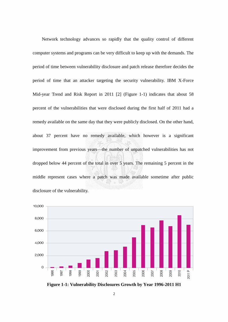
Network technology advances so rapidly that the quality control of different

computer systems and programs can be very difficult to keep up with the demands. The

period of time between vulnerability disclosure and patch release therefore decides the

period of time that an attacker targeting the security vulnerability. IBM X-Force

Mid-year Trend and Risk Report in 2011 [2] (Figure 1-1) indicates that about 58

percent of the vulnerabilities that were disclosed during the first half of 2011 had a

remedy available on the same day that they were publicly disclosed. On the other hand,

about 37 percent have no remedy available, which however is a significant

improvement from previous years—the number of unpatched vulnerabilities has not

dropped below 44 percent of the total in over 5 years. The remaining 5 percent in the

middle represent cases where a patch was made available sometime after public

disclosure of the vulnerability.

Figure 1-1: Vulnerability Disclosures Growth by Year 1996-2011 H1

3

According to CSI Computer Crime and Security Survey presented in 2010 and

2011 [3], there are three major types of attacks: Malware infection (67.1%), Laptop/

mobile device theft (33.5%), and phishing where represented as sender (38.9%). We

could also see in Figure 1-2 and Table 1-1 that the first two categories remain “winners”

this year, but only malware is on the rise.

4

Figure 1-2: Types of Attacks Experienced by Percent of Respondents

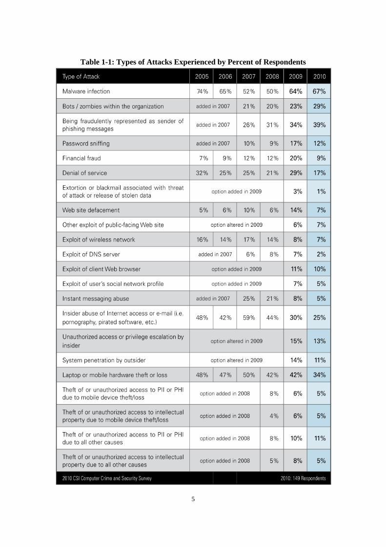
5

Table 1-1: Types of Attacks Experienced by Percent of Respondents

6

However, since the experiences, technologies, know-how, and resources have

been accumulated many years by cyber attackers, the types of cyber attacks have

changed a lot nowadays. As reported in State of Security Survey in April and May of

2011 by Symantec [4] (Figure 1-3), in Latin America, 20 percent of businesses

incurred at least $181,220 in expenses from attacks within the last year. Based on the

statistics, among the three top costs of cyber attacks to business are: Lost productivity

(36%), Lost revenue (22%), and Costs to comply with regulations after an attack

(18%). We could induce that the problem of cyber attacks are getting even worse today

and which should be highly concerned.

Figure 1-3: Costs of Cyber Attacks

As observed in IBM X-Force Mid-year Trend and Risk Report in 2011 [2], we

13%

16%

16%

16%

17%

17%

17%

18%

21%

22%

36%

0% 5% 10% 15% 20% 25% 30% 35% 40%

We don't know what was taken or impacted

Litigation costs

Reduced stock price

Direct financial cost (money or goods)

Loss of organization, customer, or employee…

Damaged brand reputation

Regulatory fines

Loss of customer trust/damaged customer…

Costs to comply with regulations after an…

Lost revenue

Lost productivity

7

might notice that there are various attacker types and techniques thriving through these

years (Figure 1-4). Some network attackers break into as many computer systems as

possible regardless of where they exist; while others are targeted in penetrating specific

victim networks that attract their interests. Some botnet operators lack sophisticated

technical skills and mostly know how to use a tool chest of exploit and malware kits

they have purchased; while others work in well-organized, state-sponsored teams that

discover new vulnerabilities and develop totally unprecedented attack techniques. Over

all, external threats can be classified based on the object of their attacks as well as how

sophisticated their attacks are.

Figure 1-4: Attacker Types and Techniques 2011 H1

Among these attacker fashions, “Cyberwar” is now a notable attacker type, which

is an Internet-based conflict involving politically motivated attack on information and

8

information systems. There are several reasons to mount a cyberwar: one is for stealing

the secrets of military affairs, politics, diplomacy, technology, or business; another is

for pure destructions or producing terrorist attacks. The goal of the latter might be

destroying political military information system or other essential national

infrastructures, like electrical power grids, oil refineries, petroleum pipelines, traffic

control systems, or financial security systems, in order to paralyze the opposite side’s

politics, military affairs, economics, or business operations and finally induce social

fear and anxiety. As a matter of fact, information security issues now have been raised

from personal and organizational levels to national level.

From the discussions and statistics above, we may gradually realize that with the

increase in complexity, scale, and speed of networks, network performance under

attacks, random failures, or accidents has become a great concern in the network

security. The degree to which a system or a network is able to provide critical services

under the pressure of various kinds of natural and artificial disasters is broadly defined

as survivability. How to evaluate the survivability of a huge network can be viewed as

an important issue. Therefore, this research is going to introduce the definitions and

measures of network survivability in the following sections.

9

1.2 Motivation

At present, network survivability is becoming an important issue of network

security technology. Numerous studies have been devoted to defining the meaning of

network survivability and estimating the impact of external and internal factors on the

network survivability [12][13]. When evaluating the survivability of a network, the

mathematical programming approaches such as game theory [14][15], Lagrangean

Relaxation Method [16][17], etc. would be the most significant work, which may carry

out the precise description and formal analysis for the dynamic behavior of network

system through the attack-defense scenario.

When it comes to network optimization problems under the attack-defense

problems, we usually consider there are a cyber attacker and a network defender

interacting with each other. On one hand, the goal of the cyber attacker is to minimize

the maximum network survivability of the defender; on the other hand, the network

defender expects to maximize the minimum network survivability of his own. As a

result, the attack-defense problem becomes a min-max or max-min problem.

In addition, previous related works often consider one-round in the attack-defense

problem [14][15][16][17]. However, due to the tremendous amount of uncertainty

10

about the attacker’s behaviors, e.g., motivations, preferences, actions, the types of

attacks, attack prediction is a very challenging task and should be observed for a long

time. Moreover, defense strategies against intentional attacks can influence the

adaptive strategy of the attacker, and vice versa. In order to achieve the goal of

maximizing or minimizing the network survivability, both of the cyber attacker and the

network defender might consider carefully how to allocate or even reallocate their

limited resources, which should be estimated to take several rounds of interactions in

reality. As a result, it is necessary to develop the concept of multi-round attack-defense

scenario analysis in our work.

How to evaluate the network survivability is a critical issue in the attack-defense

model. Traditionally, the Degree of Disconnectivity (DOD) metric which was proposed

in [17] is used to measure the damage degree of a network. However, the DOD metric

is used under the assumption that the attack is either successful or unsuccessful, which

ignores the attack might not be 100% successful or unsuccessful. Therefore, a novel

metric which is called Average Degree of Disconnectivity (Average DOD; Average

DOD could be abbreviated to “ADOD”) proposed in [18] is adopted in our model.

Average DOD consists of the concept of attack success probability calculated by

contest success function [19] and the concept of DOD metric. The larger the Average

11

DOD value, the smaller the network survivability.

In the past, we usually consider the network security under the scope of an

enterprise or a personal computer. However, due to political reasons, we often hear

news about the information warfare between two conflicting nation-states. The former

U.S. government security expert Richard A. Clarke, in his book Cyber War (May 2010),

defines “cyberwarfare” as “actions by a nation-state to penetrate another nation’s

computers or networks for the purposes of causing damage or disruption.” [5]. In

addition, in May, 2009, American president Obama assigned White House level

security officials to help every government department set up their network security

policies and establish response mechanisms to serious network attacks. Moreover, he

also devoted his effort on raising awareness among all Americans of online threats in

order to protect national critical infrastructures, and declared a plan which is called

“Cybersecurity”. Unavoidably, the scope of network security should be extended to

national level.

In 2009, a worm named Stuxnet targeting of “high-valued” Iranian assets was first

discovered. It is the first purpose-built worm designed to attack programmable logic

controllers (PLC), industrial control systems that help run critical infrastructure

12

environments [6]. Stuxnet was designed purely to attack PLCs and cause damage to the

infrastructure they operate and, ultimately, to the people and organizations that depend

on that infrastructure.

Stuxnet is clearly an example of a stealthy worm developed by an adversary that

spent a great deal of time and money on research and development. Ever since the

discovery of the worm, there has been incessant speculation that Stuxnet is a

nation-state attack against Iranian nuclear plants. From BBC new on September 23,

2010 [7], Symantec security researcher Liam O Murchu suggested that whoever had

created the worm had put a “huge effort” into it. “It is a very big project, it is very well

planned, it is very well funded,” he said. “It has an incredible amount of code just to

infect those machines.” His analysis is backed up by other research done by security

firms and computer experts. “With the forensics we now have it is evident and

provable that Stuxnet is a directed sabotage attack involving heavy insider knowledge,”

said Ralph Langner, an industrial computer expert in an analysis he published on the

web. “This is not some hackers sitting in the basement of his parents’ house. To me, it

seems that the resources needed to stage this attack point to a nation-state,” he wrote.

The suspect has finally been confirmed in June this year, unnamed U.S.

13

government officials have told a New York Times reporter that the Stuxnet worm was

created secretively by the U.S. and Israeli intelligence agencies [8]. It is estimated that

Iran might expect a retaliatory strike to be launched against the U.S. by the Iranian

cyber army [9]. Without a doubt, the cyberwar between the U.S. and Iran has just

formally begun.

From the news that mentioned above, a nation-state cyberwar is getting more and

more sobering and unavoidable, which should be highly concerned nowadays. In

addition, there is a term best describe this kind of attack which is called Advanced

Persistent Threat (APT). APT now is frequently used as a replacement term to describe

cyberwarfare between nation-states [10]. It could be viewed as a type of collaborative

attack that includes various resourced and specialized attackers working together to

mount an attack.

As a result, from the point of view of a nation, military resources could be

allocated not only to passive defense but also to active defense which means “attack”.

Traditionally, in previous attack-defense problem, we usually consider a cyber attacker

who can only attack and a network defender who can only defense. However, under the

fact that there are both attack and defense abilities existing in the nature of a nation, it

14

is essential to transfer the traditional scenario of a cyber attacker and a network

defender into two players. Both of the two players can not only defend but also attack

at the same time [27]. Hence, we would like to consider a dual-role of each player as

an attacker and a defender.

Motivated by the reasons and previous works aforementioned, in this

attack-defense model, the scenario will consider each of the two players having the

abilities of attack and defense at the same time; furthermore, the attack behavior is

launched by collaborative attack in this model. Moreover, under the framework of a

multi-round model, resource allocation, resources reallocation, and information update

of both players in each round are also considered in this paper. The more details would

be further discussed in chapter 2.

1.3 Literature Survey

In this section, the related works of the behaviors of the dual-role of defender and

attacker in each player and collaborative attack would be discussed respectively in the

first part. In the end of the first part, there would be a short summary. Then the concept

of network survivability would be introduced in the last part.

15

1.3.1 Defender’s and Attacker’s Behaviors

In this section, the related works about the behavior of the dual-role as a defender

would be discussed in section 1.3.1.1 and section 1.3.1.2; furthermore, the behavior of

the dual-role as an attacker would be introduced in section 1.3.1.3. In the end of this

section, we would summarize the behaviors of the dual-role as an attacker and a

defender in each player.

1.3.1.1 Proactive Defense and Reactive Defense

There have been many researchers devoted to proactive defense these years, but

seldom works related to reactive defense.

Traditionally, proactive defense is regarded as a “forward-looking” approach to

mitigating security risk by examining the enterprise for vulnerabilities that might be

exploited in the future [20][21]. However, in [22], Barth and Rubinstein et al. give a

novel concept of comparing the differences between proactive defense and reactive

defense. They consider that proactive defense hinges on the defender’s model of the

attacker’s incentives. For instance, without the knowledge of the attacker’s incentives

to attack in advance, the defense budget would be equally allocated to each edge under

16

proactive defense because the edges are indistinguishable. On the other hand, reactive

defense is defined as “gradually reinforcing attacked edges by shifting budget from

unattacked edges learns the attacker’s incentives and constructs an effective defense.”

Reactive strategy is less wasteful than proactive strategy because the defender

does not expend budget on attacks that do not actually occur. Therefore, under the

assumption that the defender does not know all the vulnerabilities in the system or the

attacker’s inception, reactive defense would become an efficient strategy. These two

kinds of defense strategies would be adopted in our model.

In general, defense strategies can be conceptually categorized into active defense

and passive defense. Nevertheless, different researchers have diverse opinions of the

concepts of active defense and passive defense. According to [23], active defense

involves protect victim end before the attacks start, actively finding the possible

attacks, and traceback the real attacker. On the other hand, passive defense is taken

when the attacks are launched and the target host or network is harmed before the

attack sources can be found and controlled.

Furthermore, the distinction between active defense and passive defense is

provided in [24]. Some measures, such as protective shields, are provided by their

17

nature defense. Other measures, and especially those equipped with manpower, can

generate active defense which means exerting effort when certain conditions are

encountered. The former one belongs to passive defense while the latter one belongs to

active defense. Transparently, from the point of view of this paper, the major difference

of active defense and passive defense is whether to actively exert an action to prevent

being harmed or not.

Hence, in this paper, we would classify both proactive defense and reactive

defense into passive defense based on the perspective of [24]. Moreover, the action

measure of active defense would be further discussed in next section.

1.3.1.2 Preventive Strike

According to [25], the preventive strike can be viewed as an effective measure of

active defense aimed at destroying the potential attacker and therefore preventing the

defended object from destruction. In [28], Kroening makes a distinction between

preventive war and preemptive war. He defines that a preventive war is “initiated

inevitable, and that to delay would involve greater risk” while preemption is stated as

“an attack initiated on the basis of incontrovertible evidence that an enemy is

imminent.” In [29], Tom also defines the difference. He said that “preemptive strikes

18

are attacks to prevent an attack that seems imminent. Preventive strikes are attacks that

are in principle less urgent, in the sense that they aim, for instance, to destroy weapons

programs before they reach the production stage.”

With an historical retrospect of the military affair that Israeli air strike on the

Osiraq reactor in Iraq, the mission was not preemptive but preventive based on

Kroening’s definitions. Israeli policymakers attempted diplomatic coercion to delay

Iraq’s nuclear development before the preventive strike; meanwhile, Israeli planners

also developed a plan to destroy Osiraq. Finally, Israeli leaders bear the international

storm after the strike. Peter S. Ford [30] thus provides two conclusions: First,

preventive strikes are valuable primarily for two purposes: buying time and gaining

international attention. Second, the strike provided a one-time benefit for Israel.

Subsequent strikes will be less effective due to dispersed/hardened nuclear targets and

limited intelligence. As a result, it’s essential for a nation to decide to take this active

defense for national security purpose.

Furthermore, Levitin and Hausken et al. regard preventive strike as an active

defense strategy in [24] and [26]. They consider how a defender balances between

protecting an object passively and striking preventively against an attacker, equipped

19

with one or multiple attack facilities, seeking to destroy the object. In correspondence

with the previous works mentioned, in [27], they provide an interesting work that

directly consider a game involving two actors who fight offensively and defensively

with each other over k rounds or until one target is destroyed.

Aside from the advantages might brought by preventive strike strategy, it also

could induce a retaliation attack, which causes additional expenditure of the defender’s

resource for passive defense [25]. Hence, the optimal balance between the passive

defense and active defense would remarkably improve the network survivability under

attack.

1.3.1.3 Collaborative Attacks

Traditionally, most attacks in the cyber space are launched by individual attackers

independently even though an attack may involve many compromised computers.

However, there have been more and more researches recent years believe that the next

generation cyber attack would be collaborative attacks.

Collaborative attacks are launched by some malicious adversaries to accomplish

disruption, deception, usurpation or disclosure against the targeted networks [31]. In

20

other paper, collaborative attacks are defined as two or more types of attacks such as

the blackhole attacks and the wormhole attacks, which can attack the mobile ad hoc

network in a collaborative way [32].

In [33], Xiaohu and Shouhuai model coordinated internal and external attacks

against networked systems. In this paper, there is an external attacker that can

compromise legitimate system components or participants, which then become internal

attackers. Then the internal attackers can report to the external attacker information

such as “which other components have recently been compromised.” In the fully

sophisticated scenarios, the internal attackers may receive from the external attacker

orders such as “which components should be attacked next.” In other words, the

external attacker may be fully coordinating the attacks, and the internal attackers may

exchange information with each other.

Furthermore, [34] is the first step towards realizing and instantiating a framework

of collaborative attacks from the relevant perspectives. From the point of view of the

author, collaborative attacks in general would involve multiple human attackers or

criminal organizations that have respective adversarial expertise but may not fully trust

each other. Intuitively, collaborative attacks are more powerful than the sum of the

21

underlying individual attacks that can be launched by the individual attackers

independently, which means collaborative attacks can exhibit the “1+1>2”

phenomenon.

In 2006, the U.S. Air Force coined a term called “Advanced Persistent Threat”

(APT) [35]. According to [36], APT in industry terminology is a sophisticated, targeted

attack against a computing system containing a high-value asset or controlling a

physical system. APT often requires formidable resources, expertise, and operational

orchestration. Nation states are the most aggressive perpetrators.

Moreover, in other literature, Mandiant [37] regarded ATP as a cyber attack

launched by a group of sophisticated, determined and coordinated attackers that have

been systematically compromising a specific target’s machine or entity’s networks for

prolonged period [10]. The famous Stuxnet worm mentioned earlier is considered as a

typical APT attack according to the perspectives of several information security

professionals [6] [38].

Besides, based on [39], the U.S. National Institute of Standards and Technology

(NIST) defines APT as “an adversary that possesses sophisticated levels of expertise

and significant resources which allow it to create opportunities to achieve its objectives

22

by using multiple attack vectors (e.g., cyber, physical, and deception). These objectives

typically include establishing and extending footholds within the information

technology infrastructure of the targeted organizations for purposes of exfiltrating

information, undermining or impeding critical aspects of a mission, program, or

organization; or positioning itself to carry out these objectives in the future. The

advanced persistent threat: (i) pursues its objectives repeatedly over an extended period

of time; (ii) adapts to defenders' efforts to resist it; and (iii) is determined to maintain

the level of interaction needed to execute its objectives.”

In our research, we consider the attack-defense scenario between two

nation-states. From the attack aspect of a nation-state, there must exist every kind of

talented experts specialize in information and network security who can be formed as a

group to dedicate their effort to protect their nation-state. According to the literature

that we surveyed, APT would be suitable to describe this kind of scenario; however,

APT actually could be viewed as a specific type of collaborative attacks whereas the

range of collaborative attacks to consider would be much broader. Therefore, in order

to make our model more generic, we would like to adopt the concept of collaborative

attacks into our model.

23

1.3.1.4 Summary

In our research, one of the significant contributions is that we consider the

dual-role of each player as a defender and an attacker. Hence, we are going to

summarize the behaviors aforementioned of the attack-defense dual-role. The details

are listed in Table 1-2.

Table 1-2: The Summary of the behaviors of the Attack-Defense Dual-Role

Defender’s behavior Attacker’s behavior

Proactive Defense

Reactive Defense

Preventive Strike

Collaborative Attack

1.3.2 Network Survivability

The definition of network survivability has been discussed many years. To the

best of our knowledge, the first formal definition of survivability was proposed by

Consultative Committee for International Telegraph and Telephone (CCITT) in 1984

[11]. Survivability is defined as “ability of an item to perform a required function at a

given instant in time after a specified subset of components of the item to become

24

unavailable.”

In 2004, Westmark [12] tried to provide a template for defining survivability to

facilitate subsequent research into computational quality attributes by using standard

definitions. According to Westmark, survivability is “the ability of a given system with

a given intended usage to provide a pre-specified minimum level of service in the event

of one or more pre-specified threats.”

In fact, the concept of the network survivability has been applied to evaluate the

degree of the network security for many years. However, when surveying the related

works about network security, we may find that there is no precise and uniform

definition for network survivability until now.

Among these various definitions of network survivability, one of the more cited

definitions of survivability would be what provided by Ellison [13]. The researcher

defines survivability as the “capability of a system to fulfill its mission, in a timely

manner, in the presence of attacks, failures, or accidents”.

In addition to the definitions of network survivability mentioned above, there are

still various definitions proposed by other authors. The other different definitions are

summarized and listed in Table 1-3.

25

Table 1-3: The Summary of Survivability Definition

No. Definition Author Year Origin

1 Survivability is the degree to which

essential functions are still available

even though some part of the system is

down.

M.S. Deutsch

and R.R. Willis

1988 [40]

2 Survivability is a property of a system,

subsystem, equipment process, or

procedure that provides a defined

degree of assurance that the named

entity will continue to function during

and after natural or man-made

disturbance.

U.S. Department of

Commerce

1996 [41]

3 Survivability is the ability of a system

to satisfy and to continue to satisfy

critical requirements in the face of

adverse conditions.

P. G. Neumann 2000 [42]

4 Survivability is if a system is complies

with its survivability specification.

J. Knight

and K. Sullivan

2000 [43]

26

5 Survivability is the degree to which a

system has been able to withstand an

attack or attacks, and is still able to

function at a certain level in its new

state after the attack.

S.D. Moitra

and S.L. Konda

2000 [44]

6 Survivability is the ability of a system

to continue operation despite the

presence of abnormal events such as

failures and intrusions.

S. Jha

and J.M. Wing

2001 [45]

7 Network survivability is the capability

to maintain network performance

against the failure of equipment.

Kerivin

and Mahjoub,

2005 [46]

8 Survivability means preserving

essential network services, even when a

part of network is compromised or

failed.

B. Bassiri

and S.S. Heydari

2009 [47]

9 Survivability is the system’s ability to

continuously deliver services in

P.E. Heegaard

and K.S. Trivedi

2009 [48]

27

compliance with the given requirements

in the presence of failures and other

undesired events.

10 Network survivability is the ability of a

network to stay connected under

failures and attacks.

F. Xing

and W.Wang

2010 [49]

While these definitions of network survivability provide a good description of the

concept of survivability, they do not have the mathematical precision to lead to a

quantitative characterization.

In [50], the authors try to propose a quantitative approach to evaluate network

survivability, and perceive the network survivability as a composite measure consisting

of both network failure duration and failure impact on the network. And in [51], the

paradigm that can simultaneously unify the qualitative and quantitative analysis into

the formal modeling has been proposed. The authors formally model and analyze the

survivability of network system.

Moreover, in [17], this paper presents a mathematical programming problem,

which adopts a novel metric called Degree of Disconnectivity (DOD) to evaluate the

28

damage level and survivability of a network. Furthermore, a new survivability metric is

provided in [18]. The survivability metric called Average DOD combining the concept

of the probability calculated by contest success function with the DOD metric. The

combination of the two concepts provides an efficient and powerful evaluation to solve

the quantitative analysis of network survivability. Therefore, the Average DOD metric

would be adopted in our model, and further discussions about the concept of Average

DOD would be explained and illustrated in section 2.

1.4 Thesis Organization

The rest of the paper is organized as follows. In chapter 2 we explain and

illustrate the concept of the Average DOD. In addition, the two players’ network

attack-defense scenario and formulation of this problem are introduced as well. In

chapter 3, the solution approach using the gradient method and game theory would be

discussed, and in chapter 4, the computational experiment results would be presented.

In the end, we conclude the paper and further discuss future work in chapter 5.

29

Chapter2 Problem Description

In this chapter, the concepts and calculating methods of Degree of

Disconnectivity (DOD), contest success function (CSF), and Average Degree of

Disconnectivity (Average DOD) would be introduced in the following parts. Then, the

problem description and the related problem assumptions would be described in detail

in section 2.4 and section 2.5 respectively. In the end, we would go to propose our

mathematical formulation.

2.1 Degree of Disconnectivity

In [17], the author proposed a novel metric of network survivability called Degree

of Disconnectivity (DOD) to evaluate the damage level and survivability of a network.

The definition of DOD is defined as below:

No. of broken nodes on the shortest path of each O-D pair

No. of all OD pairs of a network DOD

.

The DOD value could be explained as the average number of broken nodes in

30

each O-D (Origin-Destination) pair of a network. The larger the DOD value, the

smaller the network survivability.

However, the DOD metric assumes that the cyber attacker launches the attack

either successfully or unsuccessfully. This assumption is limited to take the situation

that the attack result might not be 100% successful or unsuccessful into consideration.

Hence, the extended and revised concept of Average DOD proposed in [18] would be

further introduced in section 2.3.

2.2 Contest Success Function

A contest is a game in which the players compete for a prize by exerting effort,

money or other resources to increase their winning probability [19]. There are diverse

topics about contests including rent-seeking, tournaments, conflict, and political

campaigns have been studied. A critical component of a contest is the Contest Success

Function (CSF), which provides each player’s probability of winning as a function of

all players' efforts.

In our research, we would like to consider the attack-defense problem between the

dual-role of attacker and defender in each player. Similarly, this problem could be

31

viewed as a kind of contest between the two players. Therefore, we could use the

concept of the contest success function into predicting the winning probabilities of the

two players.

Since there are a variety of definitions of contest success function, we choose the

most common form of the contest success function which is proposed in [19]. The

definition of contest success function is shown in Table 2-1.

Table 2-1: The Definition of Contest Success Function

Definition Notation

1( , )

1 ( )

m

ii i i m m

mii i

i

as a b

ba b

a

where 0

a

s, 0

b

s, and 0m

si (ai,bi): the success probability of attacker

compromising node i

ai : the attacker’s resource allocated on

node i

bi : the defender’s resource allocated on

node i

m: contest intensity

According to Table 2-1, the vulnerability of a node is expressed as a contest

success function modeled with a common ratio form. The more attack resources

32

allocated on node i, the more attack success probability of compromising node i;

likewise, the more defense resources allocated on node i, the less attack success

probability of the cyber attacker compromising node i. In addition, the factor of contest

intensity would also influence the result of the contest success function. In [19], the

author analyzed the impact degree of different contest intensities. When m=0, no

matter how many efforts that both parties exerts, the attack success probability is

invariably 50%. When 0<m<1, it has a disproportional advantage of investing less than

the opponent. When m=1, the investments have the proportional impact on the attack

success probability. When m>1, it gives a disproportional advantage of investing more

efforts than the opponent. When m>∞, it gives a step function where “winner-takes-all”

meaning once one player invest more than the other, he would be the winner. The

impact degree of different contest intensities is summarized in Table 2-2.

Table 2-2: The Impact Degree of Different Contest Intensities

Contest Intensity Result

m=0 The success probability is invariably 50%.

0<m<1

It has a disproportional advantage of investing fewer efforts

than the opponent.

33

m=1

The investments have the proportional impact of the success

probability.

m>1

It has a disproportional advantage of investing more efforts than

the opponent.

m>∞ The contest will be winner-takes-all.

2.3 Average Degree of Disconnectivity

Average DOD is a new metric proposed in [18] that extends from the concept of

DOD metric. The new metric combines the concept of the probability being calculated

by contest success function with the concept of DOD metric. Further details about the

concept of Average DOD are described in the following section.

2.3.1 Illustration

In this section, the concept and method to calculate the Average DOD value are

introduced and some examples are illustrated as well. In Figure 2-1, it shows that the

network is intact. Besides, every two network nodes would form an O-D pair.

Therefore, the total number of the O-D pair would be C2n (Where n is the number of

network nodes).

34

Figure 2-1: An Example of the Intact Network

In order to compromise and protect the network, both the cyber attacker and the

network defender would allocate their attack and defense resources respectively on

each node based on their strategies. Figure 2-2 represents the situation of attack and

defense resources allocating on each node. It shows that there are five nodes being

separately allocated attack resources by the cyber attacker and defense resources by the

network defender. According to Figure 2-2, the shape of triangle represents the defense

resources allocated to the node. On the other hand, the attack resources allocated to the

node is expressed as the shape of square.

Figure 2-2: The Allocated Resources on Each Node

35

Based on the resources that the cyber attacker and network defender allocate on

each node, the contest success function would be adopted to calculate the attack

success probability of each node. As the result, the attack success probability of each

node is demonstrated in Figure 2-3, where Si represents the attack success probability

of node i .

After one time of attack-defense interaction, each node of the network would

always be only two kinds of network configuration. One is still functional and the

other one is dysfunctional. The total number of all possible network configurations

would be 2 to the power of total number of network nodes ( Where n means the total

number of network nodes). For example, in Figure 2-3, the total number possible

outcome of network would be 32 (25

= 32 Where n equals 5).

Figure 2-3: The Attack Success Probability of Each Node

n2

36

Furthermore, each possible network configuration would have a probability which

is determined by the attack success probability or attack failure probability of each

node. The method to calculate the probability of each possible network configuration

would be to multiply the attack success or failure probability of each node respectively.

As a result, for example, in Figure 2-3, if all the nodes of the network are compromised

by the attacker, the probability of this network configuration would be ∏ Si5i=1

(Where Si represents the attack success probability of node i). On the other hand, if all

the nodes of the network are still functional, the probability of this network

configuration would be ∏ (1-Si)5i=1 .

Moreover, each kind of network configuration would lead to different damage

degree of network. The Degree of Disconnectivity (DOD) having been introduced in

the preceding part could be adopted to measure the damage degree of network. For

example, in Figure 2-3, if all the nodes of network are still functional, the DOD value

would be 0.

The probability and DOD value of each kind of network configuration are

calculated in the definition of the Average DOD. The concept of the Average DOD is

an expectation value which is the predicted mean value of the result of the experiment

37

of statistics to evaluate the damage degree of a network. The larger the Average DOD

value, the larger the damage degree of the network. Since the Average DOD value

would be affected by the attack success probability which is calculated by the attack

and defense resource allocations, Average DOD value could be adopted to find the

optimal resource allocation on each node for both of the cyber attacker and the network

defender. Table 2-3 represents an example of how to calculate the Average DOD value.

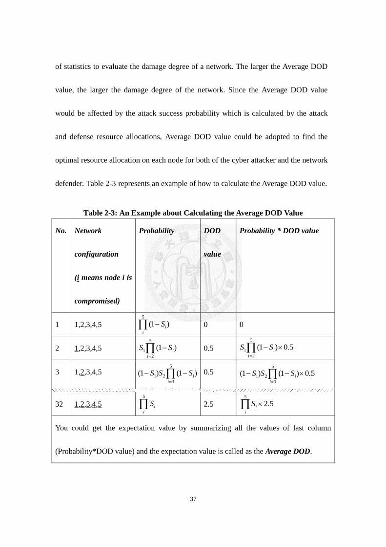
Table 2-3: An Example about Calculating the Average DOD Value

No. Network

configuration

(i means node i is

compromised)

Probability DOD

value

Probability * DOD value

1 1,2,3,4,5 0 0

2 1,2,3,4,5 0.5

3 1,2,3,4,5 0.5

32 1,2,3,4,5 2.5

You could get the expectation value by summarizing all the values of last column

(Probability*DOD value) and the expectation value is called as the Average DOD.

5

)1(i

iS

5

2

1 )1(i

iSS

5

i

iS

5

3

21 )1()1(i

iSSS

50)1(5

2

1 .SSi

i

50)1()1(5

3

21 .SSSi

i

525

.Si

i

38

2.3.2 The Calculation Procedure of the Average DOD

In the previous part, the concept and method to calculate the Average DOD value

has been introduced. Here, the calculation procedure of the Average DOD value is

summarized as below：

Step1. Finding out all the possible network configurations. The total number of

possible network configurations would be the 2 to the power of the total

number of network nodes.

Step2. Calculating the probability of each kind of possible network

configurations. Because the probability of each kind of network

configuration is determined by the attack success or failure probability of

each node, the attack success or failure probability of each node would

be multiplied as the probability of each network configuration.

Step3. Using the DOD metric to evaluate the damage degree of network of each

possible network configuration.

Step4. Using the concept of expectation value combining the probability with

the DOD value of each possible network configuration to evaluate

damage degree of whole network. The calculated expectation value

39

2.4 Problem Description

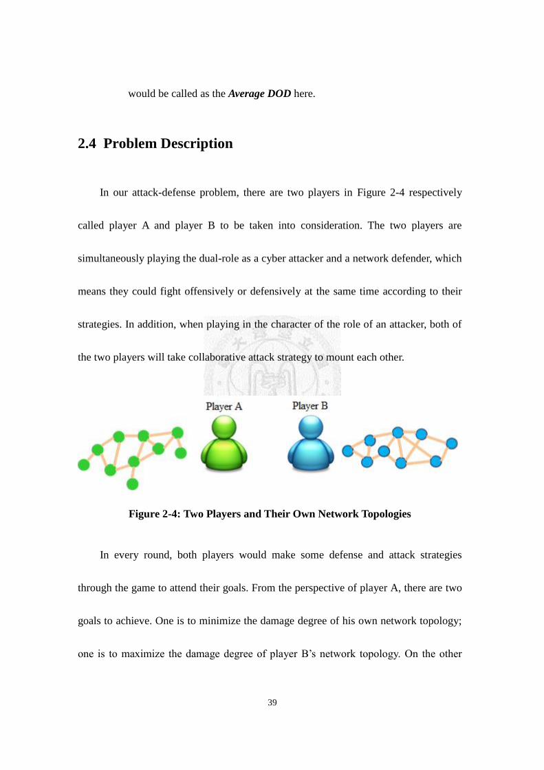
In our attack-defense problem, there are two players in Figure 2-4 respectively

called player A and player B to be taken into consideration. The two players are

simultaneously playing the dual-role as a cyber attacker and a network defender, which

means they could fight offensively or defensively at the same time according to their

strategies. In addition, when playing in the character of the role of an attacker, both of

the two players will take collaborative attack strategy to mount each other.

Figure 2-4: Two Players and Their Own Network Topologies

In every round, both players would make some defense and attack strategies

through the game to attend their goals. From the perspective of player A, there are two

goals to achieve. One is to minimize the damage degree of his own network topology;

one is to maximize the damage degree of player B’s network topology. On the other

would be called as the Average DOD here.

40

hand, player B at the same time would also have the opposite goals comparing to

player A’s. Therefore, the problem that we are going to solve is a multi-objective

problem since both of the players have two goals to achieve in the meantime.

However, both players are always limited by the invested resources. How to make

the decision to efficiently and appropriately allocate defense resource to one’s own

network and attack resource to another player’s network is an extremely significant

issue for both players. Consequently, a new mathematical model to support both

players in making optimal strategies would be developed. Furthermore, a multi-round

attack-defense problem would be considered in this mathematical model. In addition,

the damage degree of both players’ networks would be evaluated by the Average DOD

value respectively. The larger the Average DOD value, the more damage degree of the

network.

In the following parts, the respective strategies that the attack-defense dual-role

would take will be introduced in detail. For simplicity, in the following introduction,

when mentioning “the defender” and “the attacker”, we mean the dual-role of each

player as the defender and the attacker.

41

2.4.1 Dual Role as a Defender

2.4.1.1 Defense Strategies

As a defender, there are three kinds of defense strategies could be considered as

follows: Proactive defense, Reactive defense, and Preventive strike.

In our scenario, we assume that the defender does not know the vulnerabilities of

his network in the first several rounds. Therefore, he might take proactive defense,

which indicates that the defender would uniformly distribute his defense resources to

each node. However, after being attack several rounds, it would be wise for him to take

another kind of defense strategy: Reactive defense.

Reactive defense would allow the defender to allocate reinforced defense

resources to compromised nodes which have already been repaired. Therefore,

resource reinforcement rate would be considered. Besides, both proactive defense and

reactive defense could be taken together in the meantime, which depends on the

defender’s decision. Furthermore, both of these two kinds of defense strategies belong

to the category of passive defense.

The third kind of defense strategy is called preventive strike, “PS” for short in the

42

following statement. When taking PS defense, the defender would allocate his defense

resources to strike on the nodes of another player’s network topology according to the

flow of the nodes, i.e. the greater flow of the node would be allocated more resources.

This defense strategy is similar to attack strategy. However, the motivation of PS is for

defending his own network. Therefore, PS is categorized into active defense.

After the defender taking PS defense this round, the counterpart must retaliate in

the next round. Nevertheless, PS defense would cause damage to another player’s

network infrastructure and consequently indirectly influence his retaliation ability in

allocating his attack resources in the next round, which is called after-strike effect.

2.4.1.2 Resource Reallocation and Node Repairing

The defender could reallocate his defense resource in every round. However, due

to the procedure of resource shifting from one side to the other side, part of the

resources would be discounted when reallocating the defense resource. Therefore, the

discount factor of resource reallocation should be considered.

Moreover, the defender could decide to repair the broken nodes or not in every

round. If the defense resource is sufficient, the nodes compromised last round would be

43

repaired in this round. On the other hand, if the defense resource is insufficient, the

defender would choose not to repair.

Each node in defender’s network topology has a reward. The concept of reward

would be further discussed in the following section. Once the node being compromised,

the reward would be gained by the attacker; nevertheless, once the compromised node

being repaired in the next round, the reward would be retrieved back.

2.4.1.3 Updating Information: Unknown Vulnerabilities

In the beginning of the game, the defender is assumed that he does not know

where the vulnerabilities would be in his network. However, after the vulnerable nodes

are attacked, he could then update his information about the unknown vulnerabilities

existing in his network topology. The information of unknown vulnerabilities is

learned by the defender due to the attack by the attacker. Therefore, updating

information could be viewed as a kind of learning. Furthermore, since the procedure of

learning does not cost any resource of the defender, we do not consider the cost of

updating information by the defender.

Once the defender updates his information, in the next round, he would repair the

44

vulnerable nodes and then reinforce more defense resource on the repaired nodes,

which is what we mentioned previously the reactive defense.

2.4.2 Dual Role as an Attacker

2.4.2.1 Collaborative Attacks

The concept of collaborative attack is considered in our attack-defense problem.

Therefore, in our model, there would be several collaborative attackers grouped

together to mount an attack in every round.

Some of the collaborative attackers are more specialized; some are not so

specialized but have various kinds of information about the defender. Therefore, each

attacker’s attack power over a node would be different. We further assume that the

collaborative attackers’ goals are the same; meanwhile, they would share their

information to each other without concealment.

In addition, there is always existing one leader in the group in every round.

Different collaborative attackers would have different leadership. When one of the

collaborative attackers becomes the leader in that round, he might bring positive effect

or negative effect to that group, which depends on his leadership. Furthermore, this

45

leadership would affect the synergy of each attacker in that round.

When considering collaborative attacks, the effect of the collaborative attacks

would be the most critical issue to concern. Intuitively, if the attackers’ information

about the defender are all correct, it would bring them the “1+1>2” effect. On the other

hand, if some attackers have wrong information about the defender, however, they do

not know and still share with other attackers, the “1+1<2” effect would be produced.

Furthermore, some of the attackers are highly coordinated while some might be

accidentally hold the collaborative group back. Taking all these situations into

consideration, each attacker would cause different cooperative effects. Moreover, the

value of each attacker’s cooperative effect would also be different in the view of other

different collaborative attackers.

For each collaborative attacker, the cooperation with others would produce him a

synergy. In other words, each attacker has his own synergy. The synergy for each

attacker would be affected by the leader in that round, each attacker’s attack power,

and his cooperative effect with other attackers. The synergy of collaborative attacker

could be calculated as follows:

46

where the “each attacker” mentioned here does not include the collaborative attacker

himself.

For instance, assume that there are collaborative attackers i, j, and k forming a

group in this round. Besides, assume that collaborative attacker k is the leader and his

leadership is 1.5. From the view of collaborative attacker j, the cooperative effect of

collaborative attacker i is 0.2 and the cooperative effect of collaborative attacker k is

0.8. Nevertheless, from the view of collaborative attacker i, the cooperative effect of

collaborative attacker j might not be the same as 0.2. Given that the attack power of

collaborative attacker i and k on node l are 2 and 3 respectively, and collaborative

attacker j’s attack power on node l is 5. Therefore, the synergy for collaborative

attacker j on node l would be calculated as follows: Finally,

collaborative attacker j’s attack power on node l would become 5(0.84) = 4.2 in this

round.

Moreover, the cycle of attenuation and recovery of each collaborative attacker’s

attack power is also considered in our model. We assume that after attending a single

,attackereach ofpower attack

attacker)each ofeffect ve(cooperatiattacker)each ofpower (attack Leadership

ker

ttacborative ay of collaThe synerg

. 0.8432

3(0.8)]1.5[2(0.2)

47

round battle, the collaborative attacker’s attack power would decline; however, after

resting for one round, the attack power of the collaborative attacker would gradually

increase. For instance, if the collaborative attacker continuously attends three rounds of

battles, his attack power would decline three times by multiplying the attenuation

factor three times; however, if he then continuously takes a rest for two rounds, his

attack power would increase two times by multiplying the recovery factor two times.

Nevertheless, the speed to attenuate and the speed to recover are different; the latter is

much slower than the former.

For simplicity and clearness, in the following parts of this section, when

mentioning about the word “the attacker,” it indicates a group of collaborative

attackers.

2.4.2.2 Attack Strategies

Attack strategy is based on the attacker’s local view of the vulnerabilities on the

nodes of another player’s network topology. He would mount the attack by allocating

his attack resource to the vulnerable nodes in his local view that he might see.

Moreover, in the previous section, we have mentioned that PS strategy would

48

result in after-strike effect of another player in the next round. After-strike effect is that

when one of the players’ network topologies being preventive struck by another player

last round, his network infrastructure would be indirectly damaged. Therefore, his

retaliation ability in allocating attack resources in this round would be influenced and

the attack effect would become worse.

2.4.2.3 Rewards

It is assumed that each node on both players’ network topologies has a reward.

Once a node being compromised, the attacker would gain the reward of the node.

Reward could be viewed as the increment of additional usable resource such as a server,

etc. This kind of resource would be used in attack. Therefore, form the point of view of

the attacker, gaining rewards is a kind of learning. However, once the compromised

node being repaired by the defender, the reward would also be retrieved back.

2.4.2.4 Updating Information: Unknown Vulnerabilities and

Defender’s Private Information

The attacker would update his information as well. This information includes the

vulnerabilities on the nodes of the defender’s network topology and the defender’s own

49

private information. Since in our model, we take collaborative attack into consideration.

Therefore, in the beginning of every round, each collaborative attacker in that round

would try to extend his local view through exploration. After exploration, the

individual local views would be formed into a combined local view. The combined

local view represents the final range of nodes on the defender’s network topology that

the attacker may see in that round. Hence, updating information by the attacker would

need to spend an exploration cost. Moreover, different collaborative attackers have

different exploration costs.

Through the proceeding of the attack-defense rounds, the attacker would learn

more about the defender’s unknown vulnerabilities and the defender’s own private

information. Therefore, updating information is also a kind of learning for the attacker.

The differences between the defender’s information update and the attacker’s

information update would be illustrated in Figure 2-5. The defender updates the

unknown vulnerabilities information, whereas the attacker updates both of the

unknown vulnerabilities information and the private information about the defender.

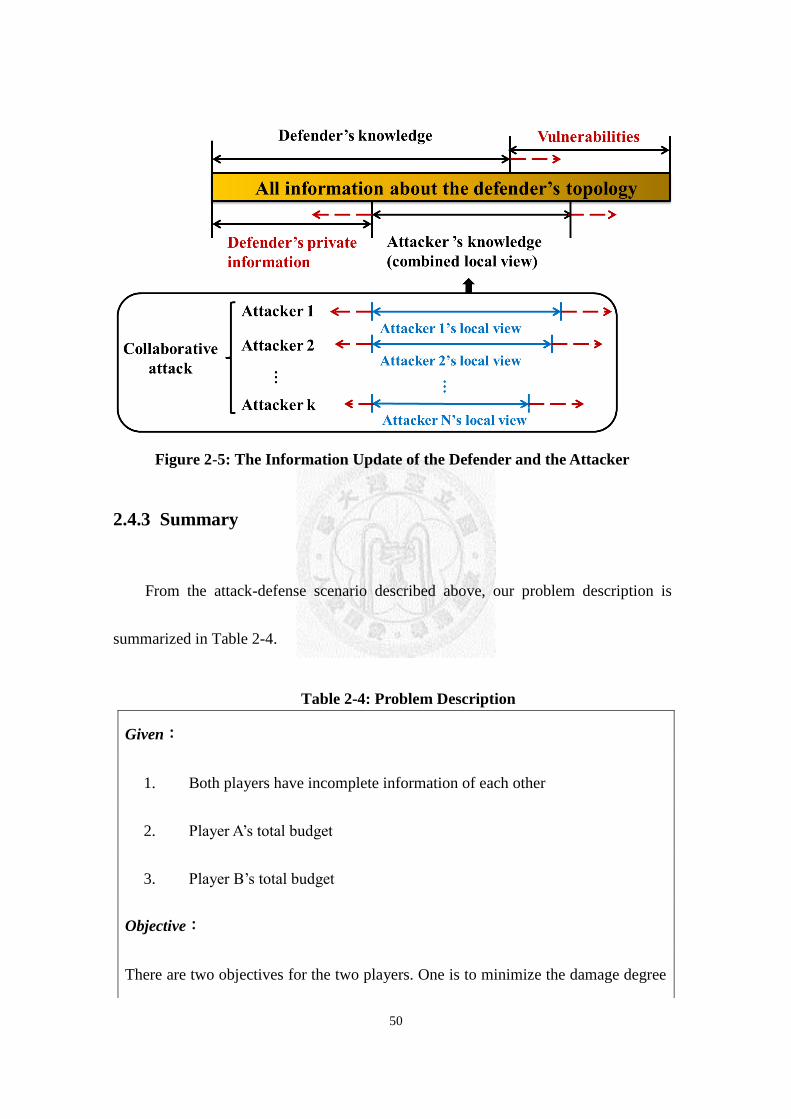
50

Figure 2-5: The Information Update of the Defender and the Attacker

2.4.3 Summary

From the attack-defense scenario described above, our problem description is

summarized in Table 2-4.

Table 2-4: Problem Description

Given：

1. Both players have incomplete information of each other

2. Player A’s total budget

3. Player B’s total budget

Objective：

There are two objectives for the two players. One is to minimize the damage degree

51

of their own network topologies; one is to maximize the damage degree of another

player’s network topologies. The Average DOD value would be used to evaluate the

damage degree of the network. In addition, player A and player B would have their

own Average DOD values according to the damage degrees of their networks.

Subject to：

1. The total budget constraint of player A.

2. The total budget constraint of player B.

To determine：

1. Player A needs to determine how to allocate the defense budget on the

nodes of his own network topology according to his passive defense

strategy and on the nodes of player B’s network topology according to his

active defense strategy. In addition, player A also needs to determine how

to allocate the attack budget on the nodes of player B’s network topology.

2. Player B needs to determine how to allocate the defense budget on the

nodes of his own network topology according to his passive defense

strategy and on the nodes of player A’s network topology according to his

active defense strategy. In addition, player B also needs to determine how

to allocate the attack budget on the nodes of player A’s network topology.

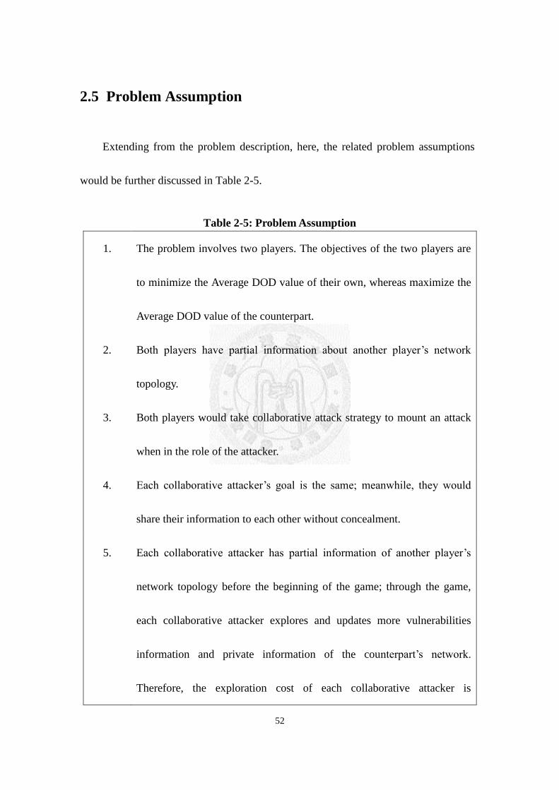
52

2.5 Problem Assumption

Extending from the problem description, here, the related problem assumptions

would be further discussed in Table 2-5.

Table 2-5: Problem Assumption

1. The problem involves two players. The objectives of the two players are

to minimize the Average DOD value of their own, whereas maximize the

Average DOD value of the counterpart.

2. Both players have partial information about another player’s network

topology.

3. Both players would take collaborative attack strategy to mount an attack

when in the role of the attacker.

4. Each collaborative attacker’s goal is the same; meanwhile, they would

share their information to each other without concealment.

5. Each collaborative attacker has partial information of another player’s

network topology before the beginning of the game; through the game,

each collaborative attacker explores and updates more vulnerabilities

information and private information of the counterpart’s network.

Therefore, the exploration cost of each collaborative attacker is

53

considered.

6. The player would allocate attack resources according to his collaborative

attackers’ combined local view in that round.

7. When taking proactive defense strategy, the player would uniformly

distribute his defense resource to each node.

8. When taking reactive defense strategy, the player would allocate more

defense resource to the repaired nodes in this round. Therefore, resource

reinforcement rate is considered.

9. When taking PS strategy, the player would allocate his defense resource

to preventively strike on the nodes of another player’s network topology

according to the flow of the nodes, i.e. the greater flow of the node would

be allocated more resources.

10. After being preventively struck last round by the counterpart, the player

must take retaliation attack in this round.

11. After being preventively stuck last round, the attacked player’s network

infrastructure would be damaged and his retaliation ability on allocating

his attack resources in this round would be discounted.

12. The defense budget could be reallocated but the discount factor is also

54

considered.

13. The compromised nodes could be repaired.

14. Each node in both players’ network topologies has a reward. Once being

compromised, the reward would be gained by the counterpart; however,

once being repaired next round, the reward would be retrieved back.

15. Each collaborative attacker’s attack power over a node is different.

16. Each collaborative attacker’s cooperative effect is varied from the point

of view of other different collaborative attackers.

17. There is always existing one leader in the group of collaborative attackers

in every round.

18. Different leaders have different leadership which could be positive effect

or negative effect.

19. The synergy of each attacker would be influenced by the leader in that

round, each attacker’s attack power, and his cooperative effect with other

attackers.

20. The cycle of attenuation and recovery of each collaborative attacker’s

attack power is considered. After attending a single round battle, the

collaborative attacker’s attack power would decline; however, after

55

resting for one round, the attack power of the collaborative attacker

would gradually increase. Therefore, the attenuation and recovery factors

would be considered.

21. Both players can observe another player’s strategy in the last round.

22. Both players are not always rational, which means they might make

irrational strategies, i.e. retaliation attack.

23. Both players are limited by their total attack and total defense budget.

24. Only static network is considered (We do not consider the growth of

network).

25. Any two nodes of network could form an O-D pair.

26. Only node attack is considered (We do not consider the link attack).

27. Only malicious attack is considered (We do not consider the random

errors).

28. The attack success probability was calculated by contest success function,

considering the resource allocation on each node of both players.

2.6 Mathematical Formulation

The given parameters and decision variables of the problem are shown in Table

2-6 and Table 2-7.

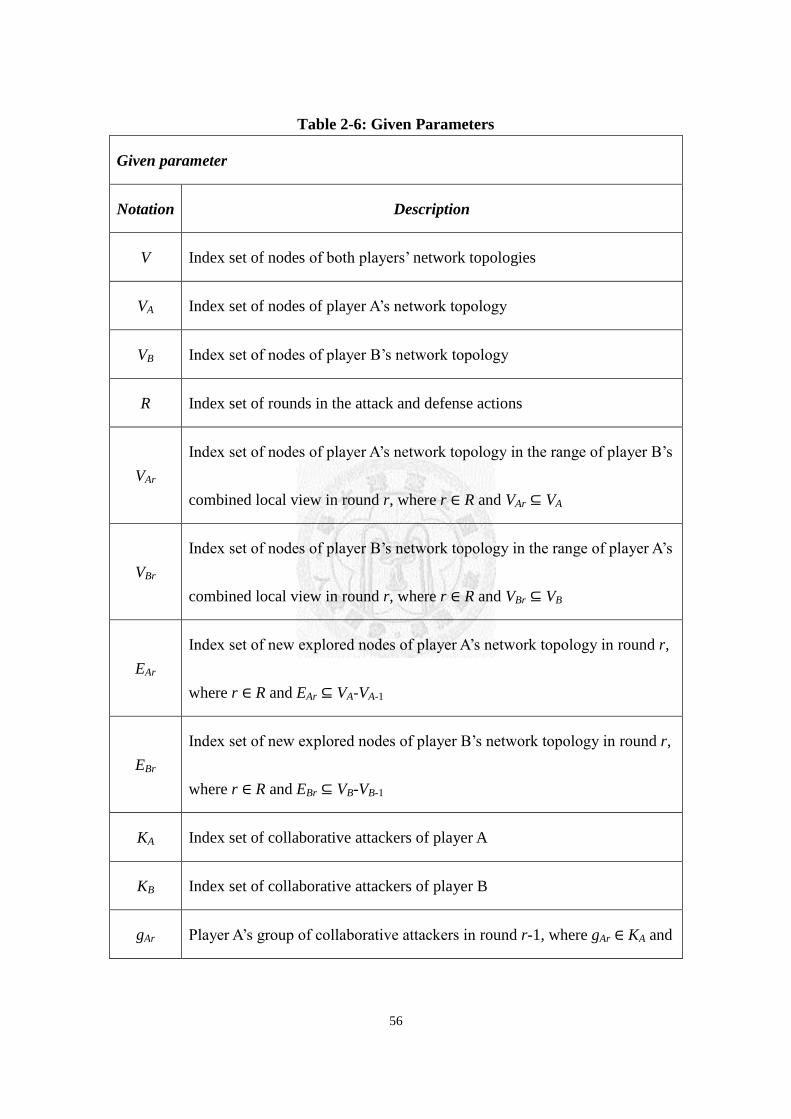
56

Table 2-6: Given Parameters

Given parameter

Notation Description

V Index set of nodes of both players’ network topologies

VA Index set of nodes of player A’s network topology

VB Index set of nodes of player B’s network topology

R Index set of rounds in the attack and defense actions

VAr

Index set of nodes of player A’s network topology in the range of player B’s

combined local view in round r, where r ∈ R and VAr ⊆ VA

VBr

Index set of nodes of player B’s network topology in the range of player A’s

combined local view in round r, where r ∈ R and VBr ⊆ VB

EAr

Index set of new explored nodes of player A’s network topology in round r,

where r ∈ R and EAr ⊆ VA-VA-1

EBr

Index set of new explored nodes of player B’s network topology in round r,

where r ∈ R and EBr ⊆ VB-VB-1

KA Index set of collaborative attackers of player A

KB Index set of collaborative attackers of player B

gAr Player A’s group of collaborative attackers in round r-1, where gAr ∈ KA and

57

r ∈ R

gBr

Player B’s group of collaborative attackers in round r-1, where gBr ∈ KB and

r ∈ R

wr The weight of the average DOD in round r, where r ∈ R

�̂� Total budget of player A

�̂� Total budget of player B

Tki

Attacker k’s capacity of attack power on node i, where k ∈ KA ⋃ KB and i

∈ VAr ⋃ VBr

tki

Attacker k’s attack power when attacking on node i in the last round, where

k ∈ gAr ⋃ g

Br and i ∈ VAr ⋃ VBr

Ckn The cooperative effect of attacker k with attacker n, where k, n ∈ KA ⋃K B

Lr

The leadership of the leader in round r, which could be positive or negative,

where r ∈ R

θi Existing defense resource allocated on node i, where i ∈ V

eri

Repair cost of players when node i is dysfunctional in round r-1, where i ∈

V and r ∈ R

dri

The discount rate of the resources that players reallocate on node i in round

r, where i ∈ V and r ∈ R

58

fri

The reinforcement rate above 1 represents the players reallocate more

resources on the repaired node i in round r, where i ∈ V and r ∈ R

lkri

Exploration cost of attacker k when information of node i is updated in

round r, where k ∈ gAr ⋃ g

Br, i ∈ EAr ⋃ EBr, and r ∈ R. The cost is greatly

increasing if the node is not adjacent with combined local view.

hkri

The discount rate of attacker k’s attack power over node i in round r, which

is gained from exploring, where k ∈ gAr ⋃ g

Br, i ∈ EAr ⋃ EBr, and r ∈ R

ui The reward of compromising node i, where i ∈ V

δri

1 if node i is compromised in round r-1, 0 otherwise, where i ∈ VAr ⋃ VBr

and r ∈ R

σr

The discount rate of the attack power in round r (after-strike effect) after

the PS of another player in round r-1, where r ∈ R

α Player A’s weight of ADOD

β Player B’s weight of ADOD

λk The attenuation factor of the collaborative attacker k, where k ∈ KA ⋃ KB

οk The recovery factor of the collaborative attacker k, where k ∈ KA ⋃ KB

59

Table 2-7: Decision Variables

Decision variable

Notation Description

yri

Proactive defense budget allocation on node i in round r, where i ∈ V

and r ∈ R

zri

PS defense budget allocation on node i in round r, where i ∈ VAr ⋃ VBr

and r ∈ R

ρAr

Player A’s group of collaborative attackers in round r, where ρAr ∈ KA

and r ∈ R

ρBr

Player B’s group of collaborative attackers in round r, where ρBr ∈ KB

and r ∈ R

sri

1 if node i is repaired by another player in round r, 0 otherwise, where i

∈ VAr ⋃ VBr and r ∈ R

Ar Total budget of player A in round r, where r ∈ R

Br Total budget of player B in round r, where r ∈ R

A⃑⃑ r

Player A’s budget allocation, which is a vector of cost A1, A2 to Ar in

round r, where i ∈ V and r ∈ R

B⃑⃑ r Player B’s budget allocation, which is a vector of cost B1, B2, to Br in

60

round r, where i ∈ V and r ∈ R

Player A’s Average DOD, which is considered under player A’s and

player B’s budget allocation on player A’s network topology in round r,

where r ∈ R

Player B’s Average DOD, which is considered under player A’s and

player B’s budget allocation on player B’s network topology in round r,

where r ∈ R

By using the above given parameters and decision variable, we then formulate the

problems as the following min-max problems respectively for player A and player B:

Objective functions:

0)(

)(

Rrr

r

rBA BD

ADwmaxmin

rr

, (IP 1)

0)(

)(

Rrr

r

rAB AD

BDwmaxmin

rr

, (IP 1’)

Subject to:

)( rAD

)( rBD

61

BrBrABrA

rBArAr

ArArArAr

ArArArAr

BrArAr

ArArArAr

ArArArAr

ABrA

Vi

rii

Vi

rii

Vi

riir

EiKk

kri

Vikgk

kri

kkik

kgk

kik

kgk

ki

knkkiknk

nkkgk

kiknk

nkkgk

ki

kkirr

Vikgk

kri

kkik

kgk

kik

kgk

ki

knkkiknk

nkkgk

kiknk

nkkgk

ki

kkirr

Vi

ririri

Vi

ri

Vi

ri

suudAl

hotott

CotCotCt

otL

htott

CtCotCt

tL

fsezy

,

),()(

)()()()(

)()()()()()(

),()(

)()()()(

)()()()()()(

ArArBArB

rABrBr

BrBrBrBr

BrBrBrBr

ArBrBr

BrBrBrBr

BrBrBrBr

BArB

Vi

rii

Vi

rii

Vi

riir

EiKk

kri

Vikgk

kri

kkik

kgk

kik

kgk

ki

knkkiknk

nkkgk

kiknk

nkkgk

ki

kkirr

Vikgk

kri

kkik

kgk

kik

kgk

ki

knkkiknk

nkkgk

kiknk

nkkgk

ki

kkirr

Vi

ririri

Vi

ri

Vi

ri

suudBl

hotott

CotCotCt

otL

htott

CtCotCt

tL

fsezy

,

),()(

)()()()(

)()()()()()(

),()(

)()()()(

)()()()()()(

AARr

r

ˆ

(IP 1.3)

BBRr

rˆ

(IP 1.4)

kikkiTt

Argk

(IP 1.5)

.kikki

Tot

Argk

(IP 1.6)

r ∈ (IP 1.1)

r ∈ (IP 1.2)

62

Explanation of the objective functions：

(IP 1) This is the objective function of player A. The ratio of player A’s ADOD

dividing by player B’s ADOD is considered in the objective function. For

player A, the ratio would be the smaller the better. Furthermore, ɑ and β

represent the importance of player A and player B respectively in each

round. The objective function of player A is to minimize the maximum sum

of the product of the ratio and weight in each round. The important degree

of Average DOD value in each round is usually different, so the weight

would be assigned to the Average DOD value in each round in this model.

(IP 1’) This is the objective function of player B. The ratio of player B’s ADOD

dividing by player A’s ADOD is considered in the objective function. For

player B, the ratio would be the smaller the better. Furthermore, ɑ and β

represent the importance of player A and player B respectively in each

round. The objective function of player B is to minimize the maximum sum

of the product of the ratio and weight in each round. The important degree

of Average DOD value in each round is usually different, so the weight

would be assigned to the Average DOD value in each round in this model.

63

Explanation of the constraint function：

(IP1.1) The constraint is for player A. In the left side of the inequality, it

represents the total budget of defense budget and attack budget in that

round. AVi

riy describes the budget of proactive defense, AVi

ririri fse is

the budget to repair compromised nodes combined with reactive defense

by reinforcing more defense budget, and the PS defense budget is

expressed as BrVi

riz ; in addition, the total attack budget in that round

should consider many factors. First, the cycle of attenuation and

recovery of each collaborative attacker is expressed as kkiλt and

kkiot

respectively, which is decided on whether to attend the attack in the last

round or not. Then, in order to consider the two discounts separately

from learning new information in that round and form player B’s PS

defense in the last round, we therefore multiply hkri for each

collaborative attacker, and in the end multiply total collaborative

attackers’ attack power by rσ . This complex item represents the total

attack power used in that round; finally, the total exploration costs of

each collaborative attacker in that round are also added to the sum. The

sum in the left side should not exceed the sum of the total budget in that

64

round, reallocated budget in that round, and the net rewards gained in

that round from the calculation of total rewards obtained from

compromising nodes in the last round minus the rewards retrieved back

when repairing compromised nodes by player B in that round.

(IP1.2) The constraint is for player B. In the left side of the inequality, it

represents the total budget of defense budget and attack budget in that

round. BVi

riy describes the budget of proactive defense, BVi

ririri fse is

the budget to repair compromised nodes combined with reactive defense

by reinforcing more defense budget, and the PS defense budget is

expressed as ArVi

riz ; in addition, the total attack budget in that round

should consider many factors. First, the cycle of attenuation and

recovery of each collaborative attacker is expressed as kkiλt and

kkiot

respectively, which is decided on whether to attend the attack in the last

round or not. Then, in order to consider the two discounts separately

from learning new information in that round and form player A’s PS

defense in the last round, we therefore multiply hkri for each

collaborative attacker, and in the end multiply total collaborative

attackers’ attack power by rσ . This complex item represents the total

65

attack power used in that round; finally, the total exploration costs of

each collaborative attacker in that round are also added to the sum. The

sum in the left side should not exceed the sum of the total budget in that

round, reallocated budget in that round, and the net rewards gained in

this round from the calculation of total rewards obtained from

compromising nodes in the last round minus the rewards retrieved back

when repairing compromised nodes by player A in that round.

(IP1.3) The constraint is for player A. Describe the sum of the total budgets in

each round should not exceed the total budgets of player A.

(IP1.4) The constraint is for player B. Describe the sum of the total budgets in

each round should not exceed the total budgets of player B.

(IP1.5) Describe the collaborative attacker’s current attack power over node i

after attending the collaborative attack in the last round should not

exceed his capacity of attack power on node i.

(IP1.6) Describe the collaborative attacker’s current attack power over node i

after taking a rest in the last round should not exceed his capacity of

attack power on node i.

67

Chapter3 Solution Approach

In this paper, there exist two players. It is notable that the problem of player A and

the problem of player B are exactly opposite; furthermore, we would have two Average

DOD values to calculate respectively for player A’s and player B’s networks. For both

players, they have their own Average DOD value according to the damage degree of

their networks. Therefore, how to optimize resource allocation of each node on the

network of their counterpart and on the network of their own and use the Average DOD

value to evaluate the survivability of their networks are needed to be solved. Hence,

the gradient method is adopted to calculate the Average DOD values and to find the

optimal resource allocation strategies on each node for both networks. Besides, we

would also combine the concept of game theory to find the optimal percentage

resource allocation in each round for both players under their individual networks.

The detailed solution procedure would be illustrated in the first section. The

concept of gradient method and the detail to calculate the Average DOD value would

be introduced in the second section. Moreover, the combination with the notion of

68

game theory would be further discussed in the third section. In the end of this chapter,

the time complexity of the solution approach would be analyzed.

3.1 The Solution Procedure

In this paper, gradient method [52] and game theory would be combined together

to find the optimal resource allocation strategy on each node in each round for both

players’ individual networks. On one hand, the gradient method would be used to

calculate the Average DOD values and to find the optimal resource allocation strategy

on each node; on the other hand, the game theory would be used to determine the

optimal percentage resource allocation in each round. The detailed process flow is

demonstrated in Figure 3-1.

Figure 3-1: The Solution Procedure of this Problem

Start

Stop

Calculating the Average DOD

value of each kind of resource

allocation

Using the gradient method to find

the optimal resource allocation

strategy on each node of each kind

of resource allocation

Finding the optimal percentage

resource allocation for both

players

Using the game theory to find the

optimal solution

69

The concept of gradient method and the application of game theory would be

introduced in the following parts.

3.2 The Calculation Method of Average DOD Value

In this section, the gradient method would be introduced first, and how to adopt

gradient method to find the optimal resource allocation strategy in each node would

then be discussed. In addition, an effective method to accelerate the calculation of

Average DOD value would also be proposed. Finally, we would demonstrate how to

calculate the Average DOD value in a multi-round attack-defense game.

3.2.1 Gradient Method

The gradient method is a general framework used to solve the optimization

problems whether to maximize or minimize functions of continuous parameters. Now,

the two problems need to be solved here are a min-max formulation for both players

and both players are assumed to allocate continuous resources on each node. Hence,

the gradient method is extremely suitable to be adopted to solve the problem.

The gradient method could be categorized into two types: One is gradient descent,

and the other is gradient ascent [52]. Both of methods could be used to solve the

optimal problems. For optimal minimization problems, the gradient descent method

70

could be adopted, whereas for the optimal maximization problems, the gradient ascent

method would be more suitable to solve. In essence, the concepts of gradient descent

and gradient ascent are greatly similar. Therefore, both of the two methods could adopt

the algorithm described in Table 3-1.

Table 3-1: The Algorithm of the Gradient Method

Step1. Get a start point

Step2. Determine a positive or negative direction

Step3. Determine a step size

Step4. Repeat

a. Find the most impact of all dimensions

b. Move a step of the most of all dimensions

c. Update the start point

Until a stop criterion is satisfied

Explanation the algorithm of gradient method：

Step1. Initially, to get a start point. The selection criterion of the start point is

important because it might influence the results and computational

efficiency.

71

3.2.2 Using the Gradient Method to Find the Optimal Resource

Allocation Strategy

The two problems in our model are both a min-max formulation and both players

are assumed that they could allocate continuous resources on each node in their own

network and in the counterpart’s network in each round. Therefore, the gradient

Step2. To determine a positive or negative direction. If the problem needs to be

solved is a maximization problem, the positive direction must be chosen.

On the other hand, when considering solving a minimization problem,

the negative direction should be chosen.

Step3. The gradient method adopts a step-by-step method to find the

optimization result. Therefore, the step size which is representative of

the move size in each step must be determined.

Step4. To determine a dimension that wants to move. The derivative method

would be used in the gradient method to find the most impact of all

dimensions. And then, moving a step of the most impact of all

dimensions and setting the new position as the next start point. And then,

repeating step 4 until the stop criterion is satisfied

72

method is extremely suitable to solve this kind of problem. However, the players’

respective two problems and the approaches to solve them are essentially the same

except for considering the different networks of the two players. Therefore, in the

following, we could consider both players’ objective functions simultaneously.

In our model, both players have a variety of defense and attack strategies which

would influence the initial resources in each round, so all of these strategies must be

taken into consideration when solving the problem by the gradient method. For both

players’ objective functions, on one hand, since the inner problem is a maximization

problem, the gradient ascent method should be adopted to solve; on the other hand, the

outer problem is a minimization problem, and therefore the gradient descent method is

suitable to solve. Nevertheless, there is still something needed to be discussed before

using the gradient method to solve our problem:

How many dimensions are there in this problem? Both players need to

determine how to allocate defense and attack resources on each node in the

network of their own and on the network of the counterpart, so the respective

number of dimensions equals to the number of nodes of their own networks.

What is the start point for both players? Both players are assumed that they

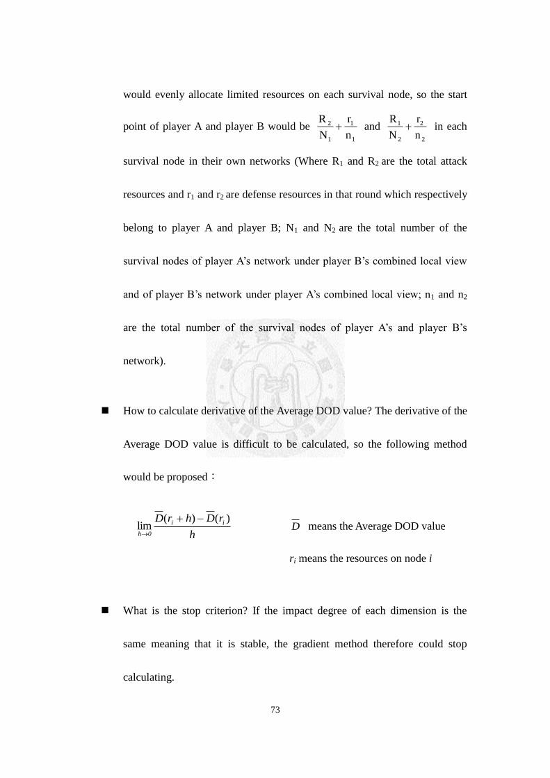
73

would evenly allocate limited resources on each survival node, so the start

point of player A and player B would be 1

1

1

2

n

r

N

R and

2

2

2

1

n

r

N

R in each

survival node in their own networks (Where R1 and R2 are the total attack

resources and r1 and r2 are defense resources in that round which respectively

belong to player A and player B; N1 and N2 are the total number of the

survival nodes of player A’s network under player B’s combined local view

and of player B’s network under player A’s combined local view; n1 and n2

are the total number of the survival nodes of player A’s and player B’s

network).

How to calculate derivative of the Average DOD value? The derivative of the

Average DOD value is difficult to be calculated, so the following method

would be proposed：

What is the stop criterion? If the impact degree of each dimension is the

same meaning that it is stable, the gradient method therefore could stop

calculating.

h

rDhrD ii

0h

)()(lim

D

means the Average DOD value

ri means the resources on node i

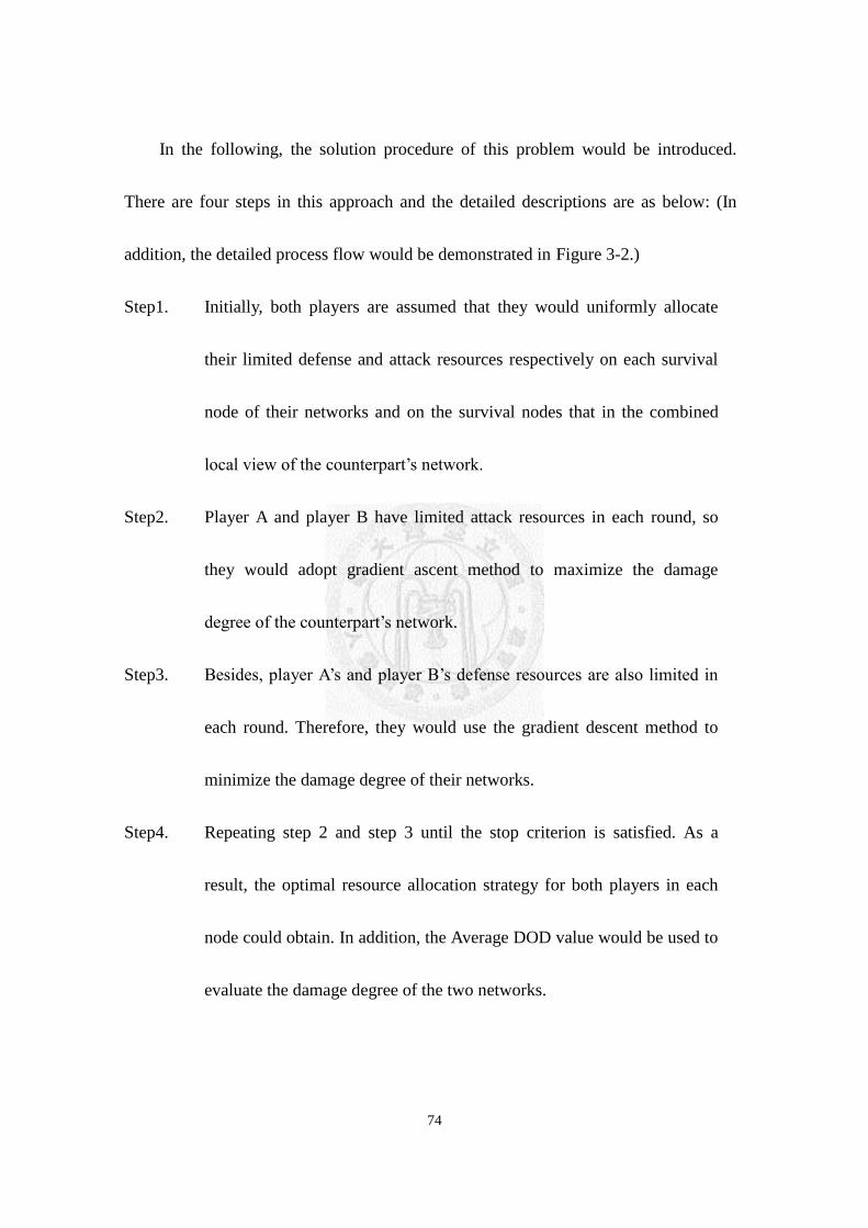
74

In the following, the solution procedure of this problem would be introduced.

There are four steps in this approach and the detailed descriptions are as below: (In

addition, the detailed process flow would be demonstrated in Figure 3-2.)

Step1. Initially, both players are assumed that they would uniformly allocate

their limited defense and attack resources respectively on each survival

node of their networks and on the survival nodes that in the combined

local view of the counterpart’s network.

Step2. Player A and player B have limited attack resources in each round, so

they would adopt gradient ascent method to maximize the damage

degree of the counterpart’s network.

Step3. Besides, player A’s and player B’s defense resources are also limited in

each round. Therefore, they would use the gradient descent method to

minimize the damage degree of their networks.

Step4. Repeating step 2 and step 3 until the stop criterion is satisfied. As a

result, the optimal resource allocation strategy for both players in each

node could obtain. In addition, the Average DOD value would be used to

evaluate the damage degree of the two networks.

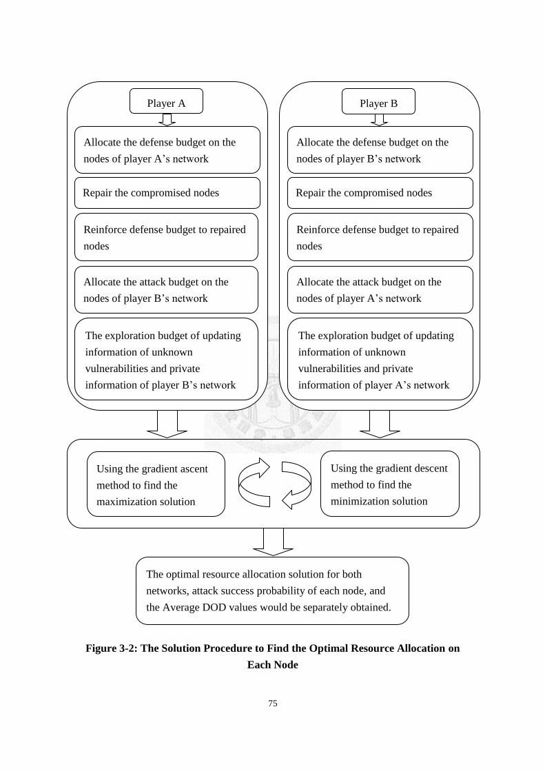
75

Figure 3-2: The Solution Procedure to Find the Optimal Resource Allocation on

Each Node

Player A Player B

Allocate the defense budget on the

nodes of player A’s network

Repair the compromised nodes

Allocate the defense budget on the

nodes of player B’s network

Repair the compromised nodes

Reinforce defense budget to repaired

nodes

Reinforce defense budget to repaired

nodes

Allocate the attack budget on the

nodes of player B’s network

Allocate the attack budget on the

nodes of player A’s network

The exploration budget of updating

information of unknown

vulnerabilities and private

information of player B’s network

The exploration budget of updating

information of unknown

vulnerabilities and private

information of player A’s network

Using the gradient ascent

method to find the

maximization solution

Using the gradient descent

method to find the

minimization solution

The optimal resource allocation solution for both

networks, attack success probability of each node, and

the Average DOD values would be separately obtained.

76

3.2.3 Accelerating Calculation of the Average DOD Value

In our problem, the Average DOD metric is adopted to evaluate damage degree of

the network. In order to obtain the Average DOD value, all the possible network

configurations are needed to be considered. In addition, once the number of network

node is too huge, it must take much time to calculate the Average DOD value.

Moreover, we have two ADOD values to be calculated in our model since we have two

network topologies to consider for both players. Therefore, an accelerating calculation

of the Average DOD value must be developed.

After analyzing the calculation of the Average DOD value, we would find that the

calculation of the probability of each network configuration is easier than the

calculation of the DOD value. As a result, a method using the probability value of each

network configuration to reduce the complexity of the calculation of the Average DOD

would be proposed.

The most critical concept in accelerating calculation of the Average DOD value is

that if the probability of the network configuration is extremely low, the impact on the

degree of the Average DOD values would be almost the same no matter how large or

how small the DOD value is. For instance, if the probability of network configuration

77

equals to 0.00000000001 and the DOD value equals to 1000 or 1, the meanings of the

respective product of the probability and the DOD value under the two situations

would be almost the same. Therefore, this feature would be applied to reduce

complexity in this model.

Consequently, the algorithm to accelerate calculation of the Average DOD value

is proposed in the following：

Step1. Calculating the probabilities of each possible network configuration.

Step2. Sorting all the possible network configurations by the probability values

from the largest to the smallest. Besides, calculating the cumulative

probability from the largest to the smallest value.

Step3. Setting a threshold of the cumulative probability. If the cumulative

probability is smaller than the threshold, calculate the corresponding

DOD value of the network configuration. Once the cumulative

probability is larger than the threshold, set the corresponding DOD value

as the largest DOD value in the network. Since when the probability is

extremely low, the impact of the degree of the Average DOD value is

almost the same no matter how large or how small the DOD value is.

78

3.2.4 The Calculation of Average DOD Value in Multi-Round

In this section, how to use the Average DOD value to evaluate damage degree of

network in multiple rounds would be introduced. In Figure 3-3, it shows how to use the

Average DOD value to evaluate damage degree of network in multiple rounds. In the

first round, both players would find the optimal strategy to allocate resources on each

node of their networks and of their counterpart’s network. After allocating resources,

each node would have a compromised probability calculated by contest success

function. As a result, there are all kinds of possibilities in the next round. Therefore,

the concept of the expected value would be adopted to calculate the Average DOD

value in the next round. Finally, combining the Average DOD value with the weight of

each round would be the final damage degree of the network. As a result, the final

Average DOD value would be W1×D̅1+∑ Wr×∑ (D̅rj×P(r-1)j)mj=0

nr=2 (Wr is the weight

of round r, D̅rj is the Average DOD value of the configuration j in round r and P(r-1)j is

the probability of the configuration j in previous round ) used to evaluate the damage

degree of network.

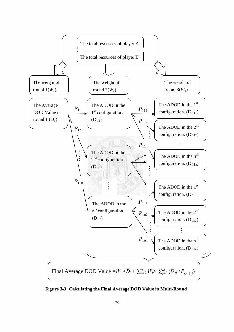
79

Figure 3-3: Calculating the Final Average DOD Value in Multi-Round

……

……

P11

……

P111 The Average

DOD Value in

round 1 (D1)

Final Average DOD Value =W1×D̅1+∑ Wr×∑ (D̅rj×P(r-1)j)mj=0

nr=2

The weight of

round 1(W1)

The weight of

round 3(W3)

The total resources of player A

The total resources of player B

The weight of

round 2(W2)

……

The ADOD in the

nth

configuration

(D 1n)

The ADOD in the

2nd

configuration

(D 12)

…

P112

The ADOD in the 1st

configuration. (D 111)

P11n

The ADOD in the 2nd

configuration. (D 112)

The ADOD in the nth

configuration. (D 11n)

P12

The ADOD in the

1st configuration.

(D 11)

P11n

…

……

P1n2

P1nn The ADOD in the nth

configuration. (D 1nn)

P1n1

The ADOD in the 1st

configuration. (D 1n1)

The ADOD in the 2nd

configuration. (D 1n2)

80

3.3 Using Game Theory to Find the Optimal Solution

In the preceding section, we used the gradient method to find the optimal resource

allocation strategy on each node for both players. However, how to efficiently allocate

total resources to each round could be another critical issue to be concerned. Hence, in

this section, the game theory would be discussed to find the optimal ratio of resource

allocation in each round for both players.

In our problem, both players need to determine how to efficiently allocate

resources simultaneously on each node in each round before the attack-defense game,

so this problem could be viewed as a simultaneous or imperfect information game [53].

In addition, both players’ gain (or loss) of utility is exactly balanced by the loss (or

gain) of the utility of the counterpart, so our problem also could be regarded as a

zero-sum game. Moreover, in [53], the definition of complete information is that

“every player knows both the strategies and payoffs (the Average DOD values in our

model) of all players in the game, but not necessarily the actions”. Therefore, although

it is definitely that both players only have partial information of the actions of each

other in our scenario, we could solve our problem with the concept of complete

information game.

81

As a result, two players, zero-sum, complete and imperfect information game

would be used to solve this problem.

Furthermore, the representation of game theory normally has two types, one is the

extensive form and the other one is the normal form. Both extensive form and normal

form could be transferred with each other. Here, the normal form would be introduced

to solve this problem in this model.

The normal form is represented by a matrix which shows the players, strategies,

and payoff values. There are two players in Table 3-2, one is on the first column and

the other is on the first row of the matrix. Both players have various kinds of different

strategies respectively. For example, in Table 3-2, they both have five different

strategies (S11 to S15 and S21 to S25). Therefore, the combination of the two players’

strategies would produce 25 (U11 to U55) different results (the Average DOD values).

Consequently, we would need to find the optimal strategy among 25 different results.

In this model, the game theory represented by the normal form could be used to

solve this problem. Both players have different strategies about the percentage resource

allocation in each round. In addition, the results of each kind of percentage resource

allocation for both players would be calculated by the Average DOD.

82

Table 3-2: An Example of the Game Theory

Strategy

Player A

S11 S12 S13 S14 S15

Player B

S21 U11 U12 U13 U14 U15

S22 U21 U22 U23 U24 U25

S23 U31 U32 U33 U34 U35

S24 U41 U42 U43 U44 U45

S25 U51 U52 U53 U54 U55

However, how to find the optimal strategies in the game theory is another issue.

Therefore, the solution approach of this game would be introduced in the following.

Generally, the solution procedure is described as below [54].

Step1. Dominated strategy eliminating. The dominant strategy means that no

matter what kind of strategy that the opponent take is better than other

strategies.

83

Step2. If only one strategy is left of each player, it would be the optimal

strategy. Otherwise, go to step 3.

Step3. Using the minmax strategy to find the optimal strategy of each player. If

minmax strategy still could not find the optimal strategy, go to step4.

Step4. Using the mixed strategy (Linear programming) to find the optimal

strategy of each player.

For example, it is a two-round attack-defense game in the Table 3-3. Both players

have 5 different strategies about allocating different resources percentage in each round.

In addition, the combined results of different percentage resource allocation strategies

for both players would be calculated by the Average DOD introduced in section 3.3.

Therefore, the solution procedure of game theory would be adopted to find the

optimal resource allocation strategy for both players in Table 3-3.

Step1. Dominated strategy eliminating. From the view of player A (player A is

assumed to be the dual-role as the attacker), player A wants to maximize

the damage degree (Average DOD) of player B’s network, so the S13 and

84

S14 strategies would be the optimal strategies. On the other hand, player

B wants to minimize the damage degree of his network, so the S25 would

be the optimal strategy. Finally, the possible results of both players

would be U53 and U54. And then, the dominated strategy eliminating

could be adopted again. The U54 would be the only one result.

Step2. Because only one result is left for each player, it would be regarded as

the optimal solution for both parties. The optimal strategy of the attacker

would be S14 and the optimal strategy of the defender would be S25.

However, if the payoff value of the U44 is 2, the optimal strategies would not be

only one. In addition, the minmax strategy also could not be used to find the optimal

strategies for both players. Therefore, the mixed strategy would be used to solve this

problem. The concept of the mixed strategy is to assign a probability to each pure

strategy and it allows each player to randomly select the pure strategy. Therefore, the

pure strategies of player A are the S13 and S14 and the pure strategies of player B are the

S24 and S25. As a result, the probability of each pure strategy of each player would need

to be found. Generally, the solution approach of the mixed strategy would use linear

programming to find the optimal solution.

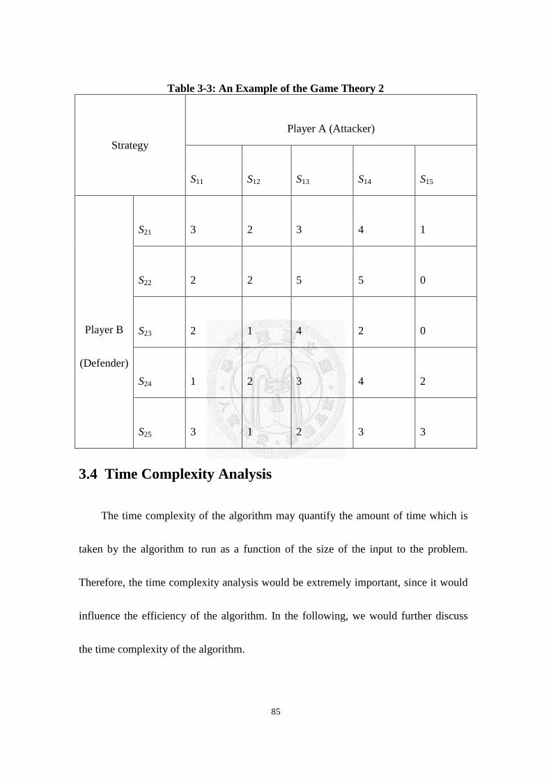
http://en.wikipedia.org/wiki/Probability

85

Table 3-3: An Example of the Game Theory 2

Strategy

Player A (Attacker)

S11 S12 S13 S14 S15

Player B

(Defender)

S21 3 2 3 4 1

S22 2 2 5 5 0

S23 2 1 4 2 0

S24 1 2 3 4 2

S25 3 1 2 3 3

3.4 Time Complexity Analysis

The time complexity of the algorithm may quantify the amount of time which is

taken by the algorithm to run as a function of the size of the input to the problem.

Therefore, the time complexity analysis would be extremely important, since it would

influence the efficiency of the algorithm. In the following, we would further discuss

the time complexity of the algorithm.

86

In our model, in order to calculate the Average DOD value, the gradient method

would be used to find the optimal resource allocation on each node. Lemma 1 states

the time complexity of gradient method.

Lemma 1 Given a total budget of both players, and a network topology, G = (V,

E), the time complexity of gradient method is O(mV).

Proof. Due to the impact degree of each node would be checked in each round,

the time complexity of the gradient method would be O(mV) (Where m is the

maximum number of the checked round and V is the number of nodes in the network).

Furthermore, the DOD value would be used to measure the damage degree of

each configuration, and all O-D pairs would be taken into calculation. Lemma 2 states

the time complexity of calculating the DOD value of each configuration.

Lemma 2 Given a network topology, G = (V, E), and using Dijkstra’s shortest

path algorithm to find all O-D pairs. The time complexity of calculating the DOD

value of each configuration is O(WV2).

Proof. The time complexity of Dijkstra’s shortest path algorithm is O(V2). After

considering all O-D pairs to calculate the DOD values of each configuration, the time

87

complexity would become O(WV2) (Where W (=C 2

V ) is the number of the O-D pairs).

In addition, to compute the Average DOD value, there are 2V different kinds of

network configuration would need to be considered. Lemma 3 states the time

complexity of calculating the Average DOD value in one round.


path algorithm to find all O-D pairs. The time complexity of calculating the Average

DOD value is O(2VWV

2) in one round.

Proof. Since there are 2V different kinds of network configuration needed to be

considered, the time complexity of calculating the Average DOD value in one round

would be O(2VWV

2) (Where W (=C 2

V ) is the number of the O-D pairs).

However, it is a multi-round attack-defense game in this model, and it must be

more complicated than only one round game. After each round of attack-defense

interaction, it would lead to 2V different kinds of network state in the new round.

Therefore, Lemma 4 states the time complexity of calculating the Average DOD value

in three rounds.


88

path algorithm to find all O-D pairs. The time complexity of calculating the Average

DOD value is O(23V

WV2) in three rounds.

Proof. In the second round, there are 2V of the Average DOD value needed to be

calculated. Furthermore, each configuration in the second round would result in 2V

kinds of network state in the third round. Therefore, 22V

of the Average DOD value

would be needed to calculate in the third round. In the end, the time complexity would

be O((22V

+2V+1)(2

VWV

2)) = O(2

3VWV

2) in three rounds (Where W (=C 2

V ) is the

number of the O-D pairs).

Besides, there is another issue about the percentage of resource allocation in each

round. Both players would have different strategies of percentage of resource

allocation in each round. Therefore, the game theory would be adopted to find the

optimal solution for both players. Lemma 5 states the time complexity of computing

the payoff values of different kinds of resource allocation strategy for both players in

three rounds

Lemma 5 Given a network topology, G = (V, E), using Dijkstra’s shortest path

algorithm to find all O-D pairs, l strategies that player A could take, and k strategies

that player B could take. The time complexity of computing the payoff values of

89

different kinds of resource allocation strategy for both players in three rounds is

O(lk23V

WV2).

Proof. Based on Lemma 4, the time complexity of calculating the Average DOD

value in three rounds is O(23V

WV2). Therefore, the time complexity of computing the

payoff values of different kinds of resource allocation strategy for both players would

be O(lk23V

WV2).

Moreover, in the proposed model, we have two networks (player A’s network

and player B’s network) to consider. Hence, the time complexity would be

O(lk23V

WV2)(2) = O(lk2

4VWV

2) in the end.

Owing to the time complexity analysis, this model could be viewed as an

extremely complicated problem. As a result, there are some restrictions would be

considered in the experiments. The detailed computational experiments would be

demonstrated in Chapter 4.

91

Chapter4 Computational Experiments

4.1 Experiment Environment

The proposed solution approach is implemented in Code Blocks and run on the PC

with AMD Phenom(tm) IIX4 B40 Processor 3.00 GHz, 6 GB RAM, and on the OS of

the MS Windows 7.

Because of the complexity of this problem, the number of network nodes

considered in the experiments is only 9 and the number of attack-defense interactions

would be discussed in only three rounds. In addition, three kinds of network topologies

are considered, the grid network (GD), the scale-free network (SF) and the random

network (RD). The feature of the GD is really regular network, and each node in the

network is connected with two neighbors along one or more dimensions. Besides, the

SF is a kind of network whose degree distribution follows a power law. Finally, the RD

is randomly connected with other nodes. Three kinds of network topologies for both

players adopted in our experiments are demonstrated in Figure 4-1, Figure 4-2, Figure

4-3, Figure 4-4, and Figure 4-5 respectively. For both players, the network topologies of

92

GD are the same while RD and SF are separate. Figure 4-2 and Figure 4-4 are for player

A; Figure 4-3 and Figure 4-5 are for player B.

93

Figure 4-1: Grid Network

Figure 4-2: Random Network A

Figure 4-3: Random Network B

Figure 4-4: Scale-Free Network A

Figure 4-5: Scale-Free Network B

94

Both players would determine how to allocate resources on each node on their own

network topologies and on the counterparts’ network topologies in each round. We

assume that in the beginning of the game, the proactive strategy would be adopted to

defense. However, in the following rounds, we would like to combine the defense

strategies of proactive and reactive. Additionally, the basic defense capability of each

survival node is 0.005.

Furthermore, in our model, both players could attack and defend at the same time.

It is notable that whether the resources should be allocated more on defense or on attack.

Therefore, we would like to discuss the impact of allocating different proportions of

attack and defense resources in our experiments. The proportion of attack resource to

defense resource for both players would be (0.3, 0.7), (0.5, 0.5), and (0.7, 0.3).

From the point of view of a nation-state, the amount of total resources could be an

important concern. The available resources would be tremendous, and the different

amounts of resources between both players might lead to a certain level of impact.

Mearsheimer proposed “Offensive Realism” in “The Tragedy of Great Power Politics”

in 2001 [56]. Offensive realism argues that great powers (powerful nation-states) ensure

their security by maximizing their share of world power [57] and explains why relations

95

between the great powers of the modern state system are fraught with conflict [58]. The

author considers that the main causes of war are located in the architecture of the

international system. What matters most is the number of powerful nation-states and

how much power each powerful nation-state controls. Therefore, he suggests four types

of systems: unbalanced bipolarity, balanced bipolarity, unbalanced multipolarity, and

balanced multipolarity. Here, bipolarity means a distribution of power in which two

nation-states have the majority of economic, military, and cultural influence

internationally or regionally [59]. Unbalanced bipolarity means the unbalanced

condition of power between two great powers; balanced bipolarity indicates the

balanced situation of power between two great powers. We consider that those

advantages of great international or regional influence could be viewed as an advantage

of a huge amount of available resources in our model. As a result, the term of “balanced

bipolarity” and “unbalanced bipolarity” would be respectively adopted in our

experiments to describe the scenarios that both players have the same amount of

resources and have different amounts of resources.

Besides, in our model, we assume that both players only know several nodes on the

counterparts’ network topologies in the first round. However, through the game, the

combined local view of known nodes would become large since both players could

96

explore new nodes in the beginning of each round. Hence, it is worthy to compare the

scenarios of incomplete information and complete information of the counterpart’s

network. We would like to know what the influence is if the player does not know every

node initially.

There is also a critical issue needed to be discussed in our experiments: The PS

strategy. The PS strategy would cause an after-strike effect. That is, when one player

takes the PS strategy to preventively strike another player, another player’s network

infrastructure would be damaged and this would indirectly influence his ability to attack

back in the next round. Therefore, we would consider the situation of taking PS and not

taking PS.

Moreover, player A’s and player B’s individual networks are described as

“Network A” and “Network B" separately in the following experiments.

The parameters used in the experiments are shown in Table 4-1.

97

Table 4-1: Experiment Parameters Settings

Parameters Value

Test Platform 1. CPU：AMD Phenom(tm) IIX4 B40 Processor

3.00 GHz

2. RAM：6GB

3. OS：MS Windows 7

Network Topology

1. Grid (In Figure 4-1)

2. Random for player A (In Figure 4-2)

3. Random for player B (In Figure 4-3)

4. Scale Free for player A (In Figure 4-4)

5. Scale Free for player B(In Figure 4-5)

Contest intensity (m) 1

The number of rounds 3

The number of nodes 9

The number of links 8~12 (GD: 12; RD: 9; SF: 8)

The number of O-D pairs 36 (considering all O-D pairs)

The total resource of both

players

160 or 120 (depends on the requirement of the

experiments)

98

4.2 Balanced Bipolarity

In this section, we would like to discuss some phenomena under the circumstance

that both players have the same amount of resources. We design three experiments, one

is about the optimal strategies for both players under complete and incomplete

information, and the other is about whether to take the PS strategy is a better decision or

not.

4.2.1 Complete and Incomplete Information

In the design of the series of this experiment, we would like to know the influence

of complete and incomplete information on both players’ strategies of percentage

resource allocation. Therefore, we are going to discuss two relative experiments as

follows: The first is the scenario of complete information and the second is the scenario

of incomplete information. Furthermore, we will make a short conclusion in the end.

4.2.1.1 Complete Information

In this experiment, both players are assumed to have complete information of the

nodes on their counterpart’s network topologies. The range of their combined local view

would be the total network topologies of each other. Therefore, the vulnerable nodes,

99

the important nodes, and the minor nodes could be recognized by both players. To

compare the results, the proportion of attack resource to defense resource that we

discussed here would be (0.3, 0.7), (0.5, 0.5), and (0.7, 0.3). Furthermore, both players’

total resources would be (160, 160), the former one is for player A, and the later one is

for player B.

The experiment results are demonstrated in Table 4-2, Table 4-3, and Table 4-4.

Table 4-2: Optimal Strategies under the Proportion of Attack to Defense Resource

is (0.3, 0.7)

Network Topology Strategy of Player A Strategy of Player B

Grid (0.5, 0.3, 0.2) (0.5, 0.3, 0.2)

Random (0.5, 0.3, 0.2) (0.5, 0.3, 0.2)

Scale-Free (0.5, 0.3, 0.2) (0.5, 0.3, 0.2)

100


is (0.5, 0.5)


Grid (0.33, 0.33, 0.34) (0.33, 0.33, 0.34)

Random (0.33, 0.33, 0.34) (0.33, 0.33, 0.34)

Scale-Free (0.33, 0.33, 0.34) (0.33, 0.33, 0.34)


is (0.7, 0.3)


Grid (0.5, 0.3, 0.2) (0.5, 0.3, 0.2)

Random (0.5, 0.3, 0.2) (0.5, 0.3, 0.2)

Scale-Free (0.5, 0.3, 0.2) (0.5, 0.3, 0.2)

Experiment Results

Under the circumstance of complete information, the optimal strategies

for both players would be (0.5, 0.3, 0.2) when the proportion of attack to

defense resource is (0.3, 0.7) and (0.7, 0.3). Moreover, the optimal strategies

for both players would become (0.33, 0.33, 0.34) in the proportion of (0.5,

101

0.5).

Discussion of Results

In the proportion of (0.3, 0.7), both players would have more defense

resources on their networks while have fewer attack resources to strike each

other. Therefore, they would like to allocate more resources in the first round

in order to have more collaborative attackers to be assigned.

In the proportion of (0.7, 0.3), both players would have fewer defense

resources on their networks while have more attack resources to strike each

other. In order to decrease the probability of being compromised, they would

allocate more resources in the first round to increase more resources for

proactive defense.

When the proportion of attack and defense resource is not equal, both

players would allocate more resources in the first round. This is due to the

reason that both players could see all the nodes on each other’s networks.

Since the attack could be more concentrated, the relative defense should be

enhanced, and vice versa.

102

In the proportion of (0.5, 0.5), the available attack and defense resources

are the same. Therefore, owing to the reason that they could see all the nodes

on each other’s networks, uniformly distributing total resources in each round

would be the optimal strategy.

4.2.1.2 Incomplete Information

In this experiment, both players only have partial information of each other’s

networks, which is the original scenario in our problem description. The range of nodes

and information in their combined local view is limited. To compare the results, the

proportion of attack resource to defense resource that we discussed here would be (0.3,

0.7), (0.5, 0.5), and (0.7, 0.3). Furthermore, both players’ total resources would be (160,

160), the former one is for player A, and the later one is for player B.

I. Optimal Strategies under Different Proportions of Attack to

Defense Resource

The experiment results are demonstrated in Table 4-5, Table 4-6, and Table 4-7.

103


is (0.3, 0.7)


Grid (0.33, 0.33, 0.34) (0.33, 0.33, 0.34)

Random (0.33, 0.33, 0.34) (0.33, 0.33, 0.34)

Scale-Free (0.33, 0.33, 0.34) (0.33, 0.33, 0.34)


is (0.5, 0.5)


Grid (0.5, 0.3, 0.2) (0.5, 0.3, 0.2)

Random (0.5, 0.3, 0.2) (0.5, 0.3, 0.2)

Scale-Free (0.5, 0.3, 0.2) (0.5, 0.3, 0.2)

104


is (0.7, 0.3)


Grid (0.33, 0.33, 0.34) (0.33, 0.33, 0.34)

Random (0.5, 0.3, 0.2) (0.5, 0.3, 0.2)

Scale-Free (0.5, 0.3, 0.2) (0.33, 0.33, 0.34)

Experiment Results

Under the circumstance of incomplete information, the optimal strategies

for both players would be (0.33, 0.33, 0.34) when the proportion of attack to

defense resource is (0.3, 0.7). The optimal strategies would become (0.5, 0.3,

0.2) in the proportion of (0.5, 0.5). Furthermore, the results are more

complicated in the proportion of (0.7, 0.3). In grid network, the optimal

strategies for both players would be (0.33, 0.33, 0.34); in random network, the

optimal strategies would become (0.5, 0.3, 0.2); in scale-free network, the

optimal strategy for player A would be (0.5, 0.3, 0.2) while the optimal

strategy for player B would be (0.33, 0.33, 0.34).

105


In the proportion of (0.3, 0.7), the defense resources would be sufficient

under the premise that the counterpart can’t not see all the nodes on the

network. From the point of view of attack, since one does not know the

information of each node on the other side, he would choose to attack

conservatively. Therefore, both players would adopt the strategy of (0.33, 0.33,

0.34) in the proportion of (0.3, 0.7).

In the proportion of (0.5, 0.5), it is a close match. The defense resources

and attack resources allocated on one network would be the same. Therefore,

as far as both players are concerned, defense is important as well as attack. On

one hand, they would prefer to allocate more resources in the first round to

enhance proactive defense and then reinforce compromised nodes by reactive

defense in the second round. On the other hand, they would like to

compromise more nodes within their combined local views as early as

possible. Furthermore, to allocate more resources as early as possible would

also help them explore new nodes. Therefore, both players would adopt the

strategy of (0.5, 0.3, 0.2) in the proportion of (0.5, 0.5).

106

The optimal strategies for both players under the proportion of (0.7, 0.3)

is seemingly more complex. The combinations of their optimal strategies

would vary from network topologies compared. However, when we further

discuss both players’ networks one at a time, we would find consistency. The

observation would be demonstrated in the following.

II. Optimal Strategies under Different Proportions of Attack to

Defense Resource and Different Networks

The experiment results are demonstrated in Table 4-8 and Table 4-9.

Table 4-8: Optimal Strategies in Network A (0.7, 0.3)


Grid (0.5, 0.3, 0.2) (0.33, 0.33, 0.34)

Random (0.5, 0.3, 0.2) (0.33, 0.33, 0.34)

Scale-Free (0.5, 0.3, 0.2) (0.33, 0.33, 0.34)

107

Table 4-9: Optimal Strategies in Network B (0.7, 0.3)


Grid (0.33, 0.33, 0.34) (0.5, 0.3, 0.2)

Random (0.33, 0.33, 0.34) (0.5, 0.3, 0.2)

Scale-Free (0.33, 0.33, 0.34) (0.5, 0.3, 0.2)

Experiment Results

Under the circumstance of incomplete information, on one hand, the

optimal strategies for both players on their own networks would be (0.5, 0.3,

0.2); on the other hand, the optimal strategies for both players on their

counterparts’ networks would be (0.33, 0.33, 0.34).


When taking only network A into consideration, the objective of player A

would be to minimize his damage degree of network while the objective of

player B would be to maximize his damage degree of network. Therefore, in

the proportion of (0.7, 0.3), player A would like to allocate more resources in

the first and the second round in order to increase his proactive and reactive

108

defense to counter player B’s attack. On the other hand, player B has limited

information on network A and has plentiful attack resources to use in the

proportion of (0.7, 0.3). As a result, player B would choose to uniformly

allocate his resources in each round. Owing to the symmetry of network B,

the analysis is vice versa.

As a result, when both players’ objectives are to maximize the damage

degree of network of the counterpart’s and minimize their own damage degree

of network at the same time, the optimal strategies for them would be either

(0.5, 0.3, 0.2) nor (0.33, 0.33, 0.33) no matter under what kind of network

topologies. If the player cares much about his own network, he would choose

the strategy of (0.5, 0.3, 0.2). Conversely, if he cares much about the other’s

network, (0.33, 0.33, 0.34) would be adopted. This phenomenon could explain

the experiment results in the proportion of (0.7, 0.3) in the previous part.

4.2.1.3 Conclusion

In complete information game, both players would be more aggressive to

allocate more resources in the first round when the attack and defense

resources are unbalanced; however, when in a close completion, they would

109

be more conservative to uniformly allocate their resources in each round.

In incomplete information game, due to the combined local views are

limited, both players would uniformly allocate when their defense resources

are more. Moreover, when in a close competition, they would allocate more in

the first round not only for defense and attack but also for exploring more new

nodes. However, when the attack resources are allocated more than defense

resources on one’s network, to allocate the resources more in the first round or

to uniformly allocate depends on whether the player cares more about defense

or attack.

4.2.2 The Effect of PS Strategy

In the design of the series of this experiment, we would like to know whether to be

the first to strike or both players to fight straightforward is a better decision. Therefore,

we are going to discuss two relative experiments as follows, and will make a short

conclusion in the end.

4.2.2.1 One Player takes PS Strategy

In this experiment, player A would take PS strategy in the first round and the

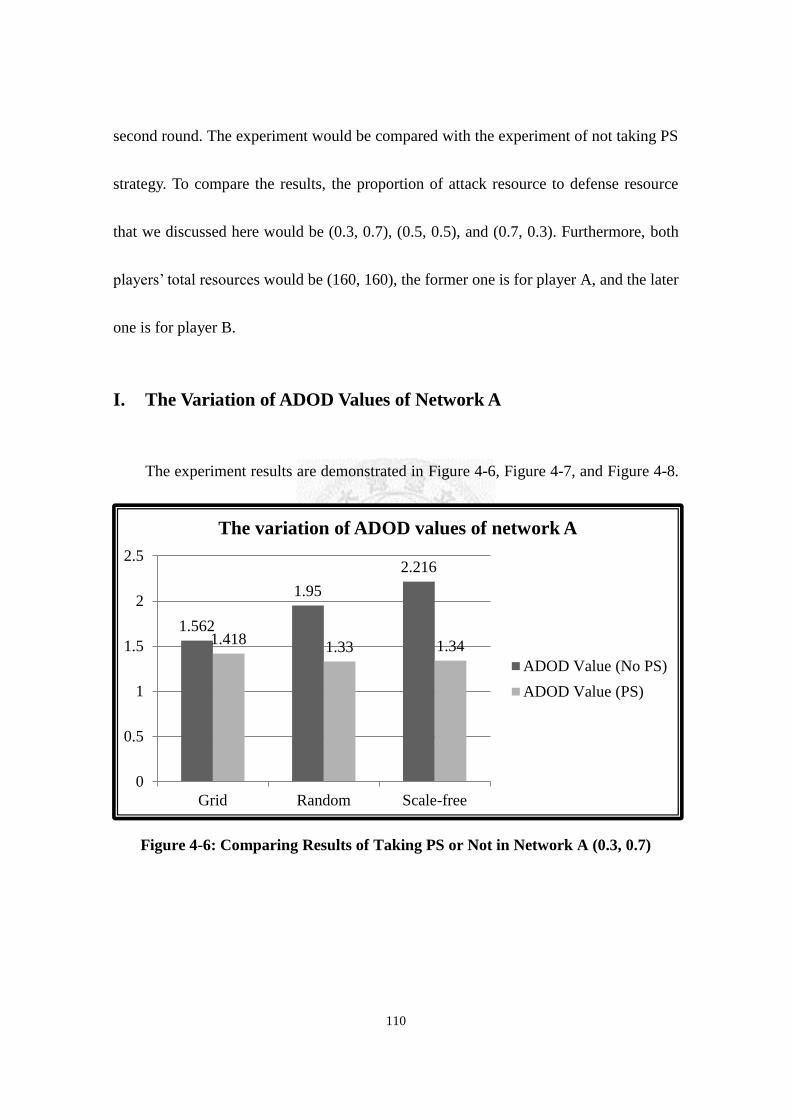
110

second round. The experiment would be compared with the experiment of not taking PS

strategy. To compare the results, the proportion of attack resource to defense resource

that we discussed here would be (0.3, 0.7), (0.5, 0.5), and (0.7, 0.3). Furthermore, both

players’ total resources would be (160, 160), the former one is for player A, and the later

one is for player B.

I. The Variation of ADOD Values of Network A

The experiment results are demonstrated in Figure 4-6, Figure 4-7, and Figure 4-8.

Figure 4-6: Comparing Results of Taking PS or Not in Network A (0.3, 0.7)

1.562

1.95

2.216

1.418 1.33 1.34

0

0.5

1

1.5

2

2.5

Grid Random Scale-free

The variation of ADOD values of network A

ADOD Value (No PS)

ADOD Value (PS)

111



Experiment Results

After player A takes PS strategy in the first and the second rounds, the

2.895

3.624

4.194

2.588

3.006 2.844

0

0.5

1

1.5

2

2.5

3

3.5

4

4.5



ADOD Value (No PS)

ADOD Value (PS)

4.945

5.662

6.225

4.606 4.24

5.045

0

1

2

3

4

5

6

7



ADOD Value (No PS)

ADOD Value (PS)

112

ADOD values of his own network topology would decrease when comparing

with the results of no one takes PS strategy.


When player A takes PS strategy in round one and round two, it would

separately produce an after-strike effect in the second and the third round. The

after-strike effect would reduce player B’s retaliation ability of using his

attack power in the following round. He can’t attack back with his full attack

power. In that way, network A would be prevented from great damage caused

by player B. As a result, the ADOD values of network A decrease.

II. The Variation of ADOD Values of Network B

The experiment results are demonstrated in Figure 4-9, Figure 4-10, and

Figure 4-11.

113

Figure 4-9: Comparing Results of Taking PS or Not in Network B (0.3, 0.7)


1.452

1.922

2.759

1.452 1.419

2.193

0

0.5

1

1.5

2

2.5

3


The variation of ADOD values of network B

ADOD Value (No PS)

ADOD Value (PS)

2.852

3.829

4.209

2.852

3.829 4.06

0

0.5

1

1.5

2

2.5

3

3.5

4

4.5



ADOD Value (No PS)

ADOD Value (PS)

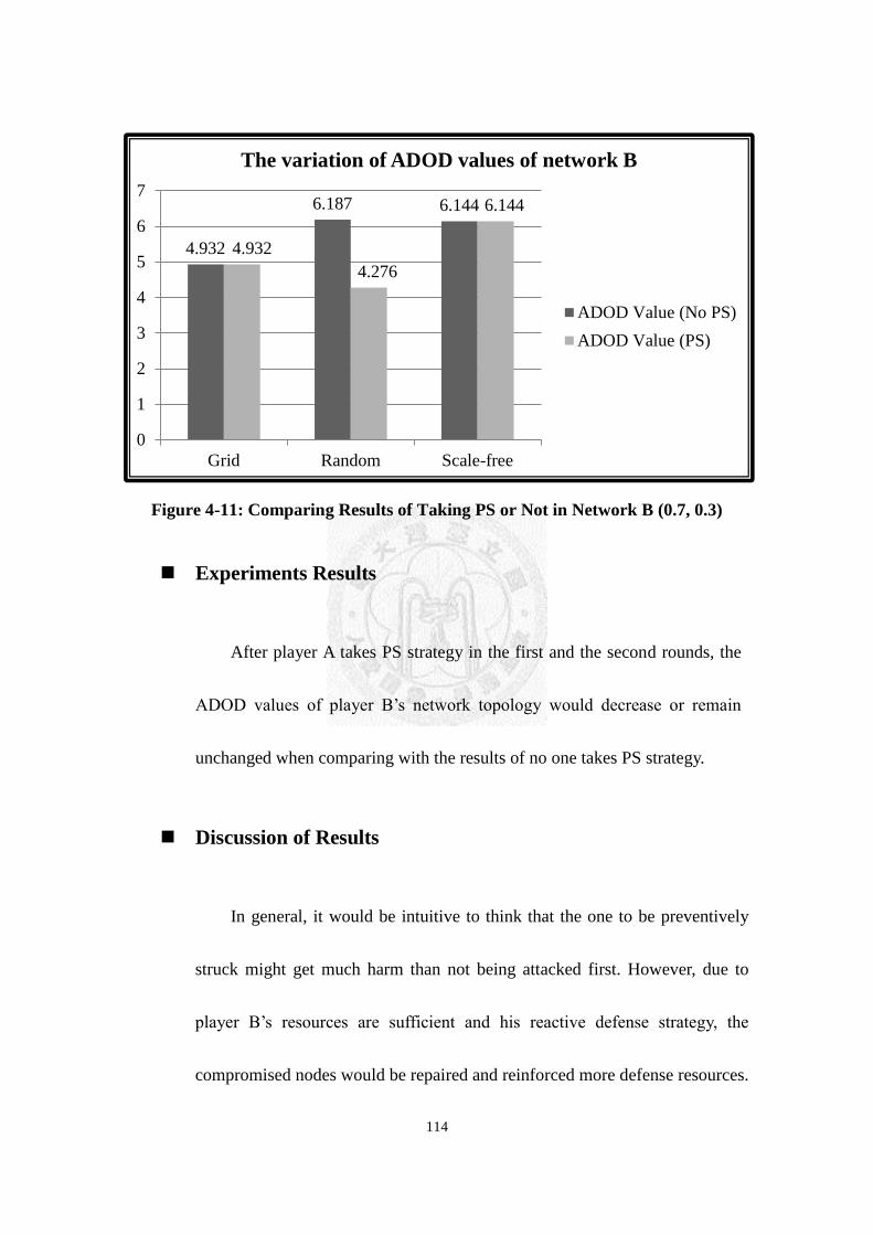
114


Experiments Results

After player A takes PS strategy in the first and the second rounds, the

ADOD values of player B’s network topology would decrease or remain

unchanged when comparing with the results of no one takes PS strategy.


In general, it would be intuitive to think that the one to be preventively

struck might get much harm than not being attacked first. However, due to

player B’s resources are sufficient and his reactive defense strategy, the

compromised nodes would be repaired and reinforced more defense resources.

4.932

6.187 6.144

4.932

4.276

6.144

0

1

2

3

4

5

6

7



ADOD Value (No PS)

ADOD Value (PS)

115

Therefore, if player A continues to attack the same nodes in the new round, it

would be no effect or even harder to compromise those nodes. In the end, the

ADOD values of network B would decrease or remain unchanged.

III. Summary

The advantage of taking PS strategy for consecutive two rounds is to protect

one’s own network topology; however, it would not cause too much damage on the

counterpart’s network topology. The counterpart’s would update his information

and know which node is important in the view of the attacker. Therefore, due to the

fruitful resources used on reactive defense, the better way to cause greater damage

might be gradually raise the total attack power in each new round.

4.2.2.2 Two Players take PS Strategy

In this experiment, player A would take PS strategy in the first round and then

player B would take PS strategy in the second round. The experiment would be

compared with the experiment of both players not taking PS strategy. To compare the

results, the proportion of attack resource to defense resource that we discussed here

would be (0.3, 0.7), (0.5, 0.5), and (0.7, 0.3). Furthermore, both players’ total resources

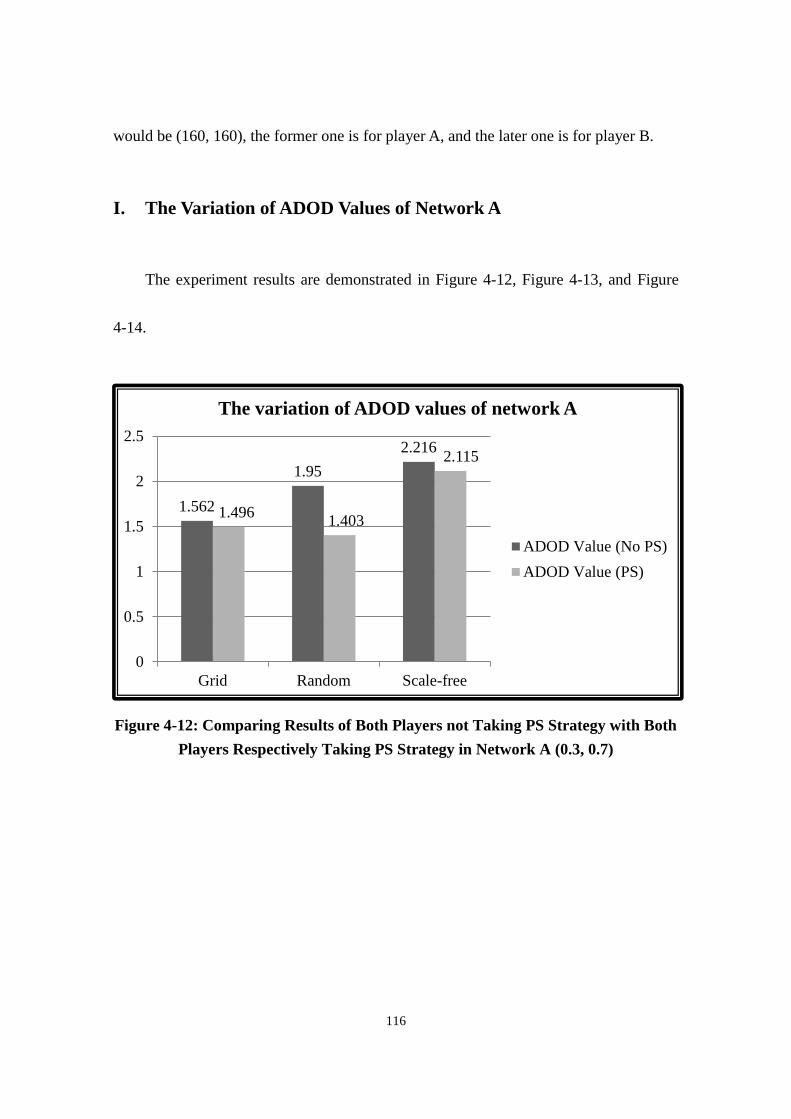
116

would be (160, 160), the former one is for player A, and the later one is for player B.


The experiment results are demonstrated in Figure 4-12, Figure 4-13, and Figure

4-14.

Figure 4-12: Comparing Results of Both Players not Taking PS Strategy with Both

Players Respectively Taking PS Strategy in Network A (0.3, 0.7)

1.562

1.95

2.216

1.496 1.403

2.115

0

0.5

1

1.5

2

2.5



ADOD Value (No PS)

ADOD Value (PS)

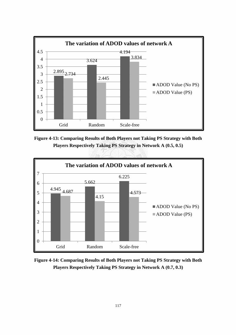
117





2.895

3.624

4.194

2.734 2.445

3.834

0

0.5

1

1.5

2

2.5

3

3.5

4

4.5



ADOD Value (No PS)

ADOD Value (PS)

4.945

5.662

6.225

4.687 4.15

4.573

0

1

2

3

4

5

6

7



ADOD Value (No PS)

ADOD Value (PS)

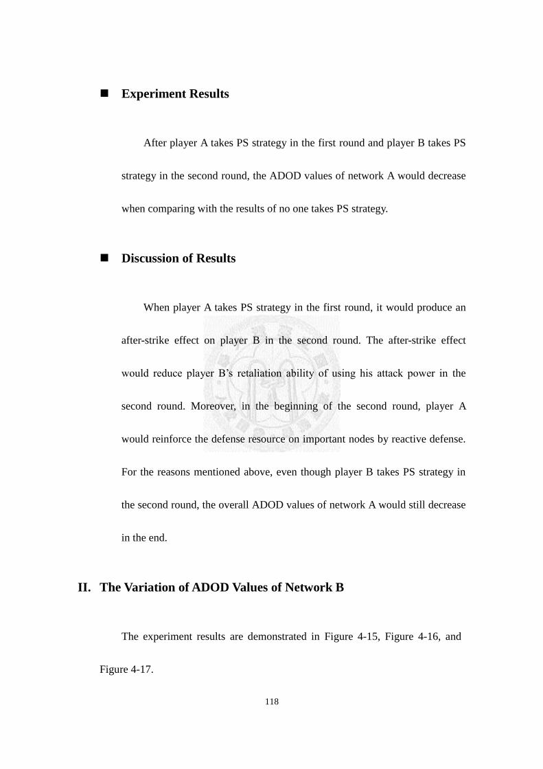
118

Experiment Results

After player A takes PS strategy in the first round and player B takes PS

strategy in the second round, the ADOD values of network A would decrease

when comparing with the results of no one takes PS strategy.


When player A takes PS strategy in the first round, it would produce an

after-strike effect on player B in the second round. The after-strike effect

would reduce player B’s retaliation ability of using his attack power in the

second round. Moreover, in the beginning of the second round, player A

would reinforce the defense resource on important nodes by reactive defense.

For the reasons mentioned above, even though player B takes PS strategy in

the second round, the overall ADOD values of network A would still decrease

in the end.


The experiment results are demonstrated in Figure 4-15, Figure 4-16, and

Figure 4-17.

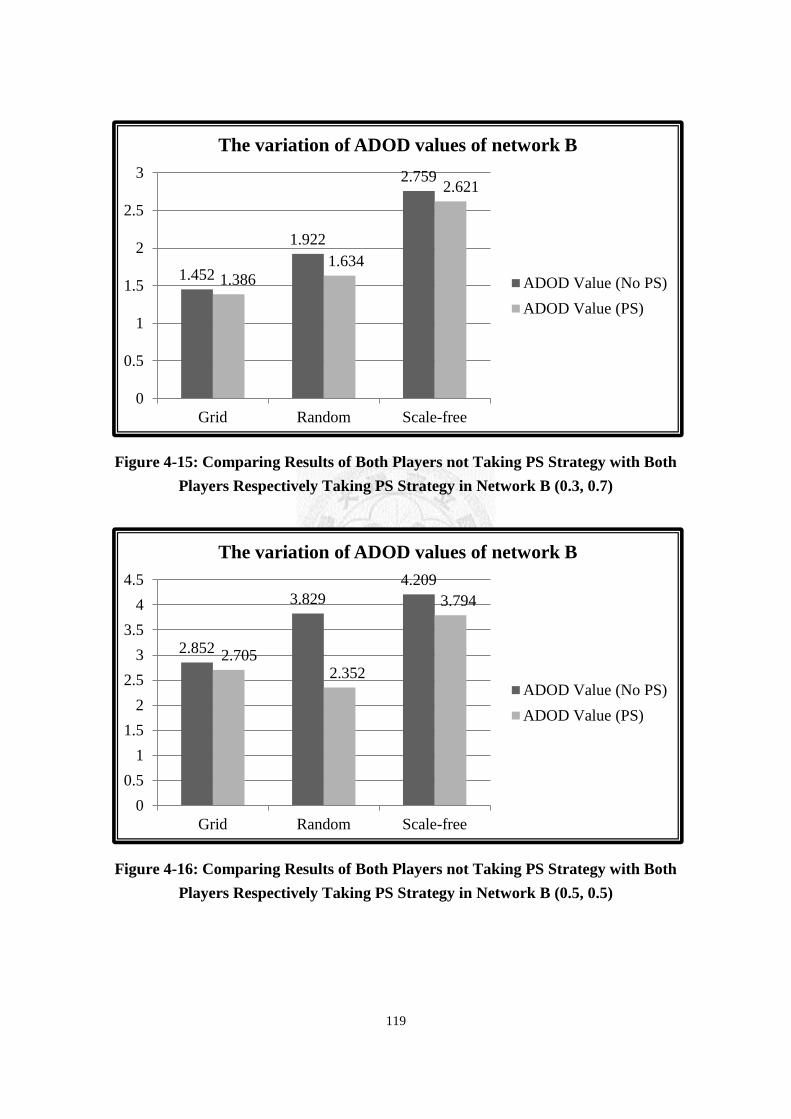
119


Players Respectively Taking PS Strategy in Network B (0.3, 0.7)



1.452

1.922

2.759

1.386

1.634

2.621

0

0.5

1

1.5

2

2.5

3



ADOD Value (No PS)

ADOD Value (PS)

2.852

3.829

4.209

2.705 2.352

3.794

0

0.5

1

1.5

2

2.5

3

3.5

4

4.5



ADOD Value (No PS)

ADOD Value (PS)

120



Experiments Results

After player A takes PS strategy in the first round and player B takes PS

strategy in the second round, the ADOD values of network B would decrease

when comparing with the results of no one takes PS strategy.


When player A takes PS strategy in the first round, player B would

update his information and then reinforce his defense through reactive

strategy in the beginning of round two. Then, player B also takes PS strategy,

4.932

6.187 6.144

4.868 4.546

5.971

0

1

2

3

4

5

6

7



ADOD Value (No PS)

ADOD Value (PS)

121

which influences player A’s use of attack power on network B in the third

round. For the reasons that the defense is reinforced and that player A’s

attack power is weakened, the overall ADOD of network B would decrease

in the end.

III. Summary

The advantage of both players to take PS strategy is to protect their own

network topologies; however, it would not cause too much damage on the

counterpart’s network topology. The relative analysis is similar to the analysis that

only one player takes PS strategy in the first round.

4.2.2.3 Conclusion

In the series of the experiments, we could make a conclusion that it would be wise

to take PS strategy. No matter there’s only one player taking PS strategy or both players

adopting this strategy, it would make the chances of their networks to survive higher.

What’s worse is that both players decide to fight straightforward without PS strategy.

Comparing with both players takes PS strategy, the damage condition of the network

when no one takes PS strategy would be much worse in the average case or at most the

122

same in the best case. Therefore, the “First-Strike” strategy is definitely valuable to be

adopted.

4.3 Unbalanced Bipolarity

In this section, we would like to discuss some phenomena under the circumstance

that both players have different amounts of resources. We design two experiments, one

is about which round should be allocated more resources, and another is about whether

to allocate more resources on attack or on defense. For the two experiments, we would

focus more on the discussions of the player who has fewer total resources.

4.3.1 Resource Allocation of Attack and Defense

In the design of the series of this experiment, we would like to know under what

kind of situations the player who has fewer resources would allocate more resources in

the first round, and under what kind of circumstances the player would choose to

allocate more resources in the last round. Therefore, we are going to discuss two relative

experiments as follows, and will make a short conclusion in the end.

4.3.1.1 Resource Allocation Ratio under Attack to Defense is 0.3: 0.7

In this experiment, we consider that player A and player B have different amounts

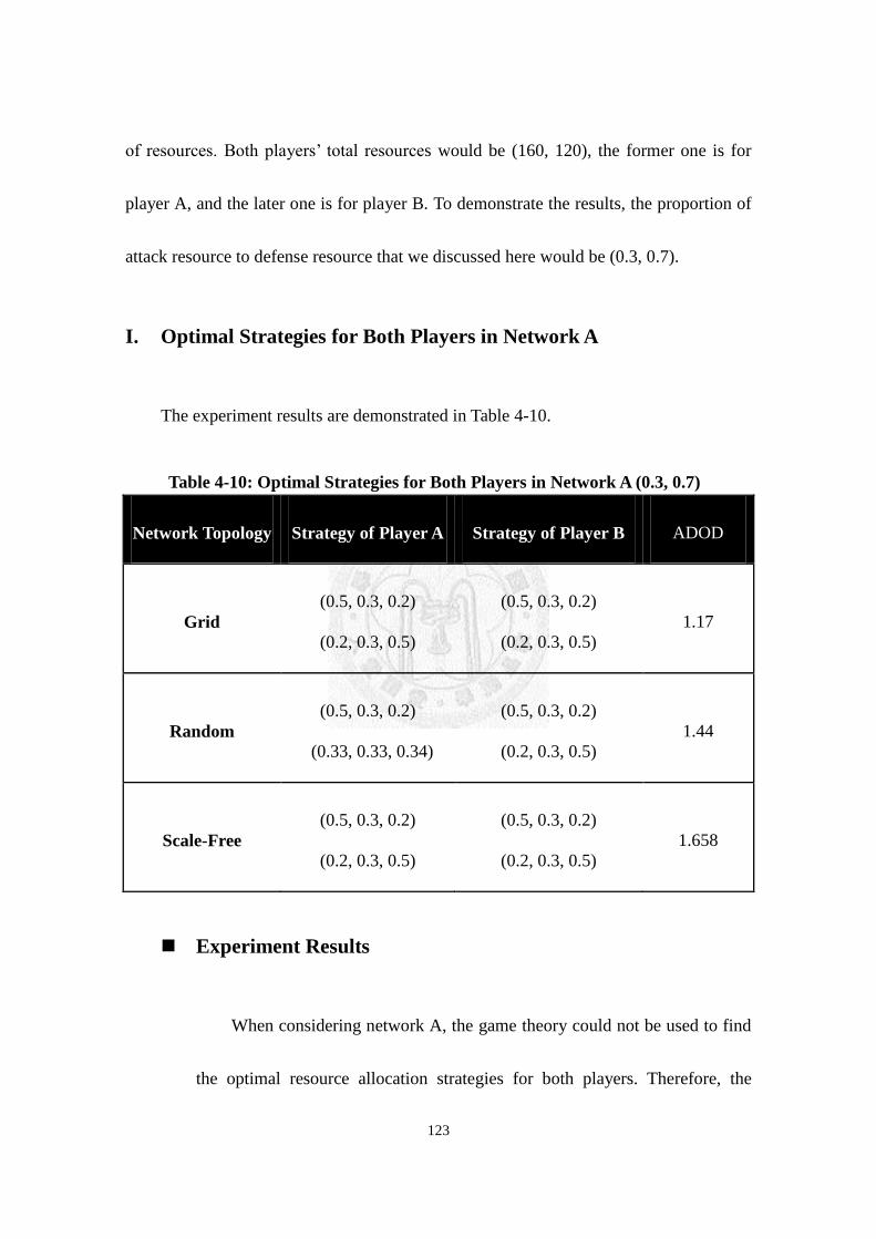
123

of resources. Both players’ total resources would be (160, 120), the former one is for

player A, and the later one is for player B. To demonstrate the results, the proportion of

attack resource to defense resource that we discussed here would be (0.3, 0.7).

I. Optimal Strategies for Both Players in Network A

The experiment results are demonstrated in Table 4-10.

Table 4-10: Optimal Strategies for Both Players in Network A (0.3, 0.7)

Network Topology Strategy of Player A Strategy of Player B ADOD

Grid

(0.5, 0.3, 0.2)

(0.2, 0.3, 0.5)

(0.5, 0.3, 0.2)

(0.2, 0.3, 0.5)

1.17

Random

(0.5, 0.3, 0.2)

(0.33, 0.33, 0.34)

(0.5, 0.3, 0.2)

(0.2, 0.3, 0.5)

1.44

Scale-Free

(0.5, 0.3, 0.2)

(0.2, 0.3, 0.5)

(0.5, 0.3, 0.2)

(0.2, 0.3, 0.5)

1.658

Experiment Results

When considering network A, the game theory could not be used to find

the optimal resource allocation strategies for both players. Therefore, the

124

mixed strategy would be adopted to find the optimal resource allocation

strategies for both players.

In the grid network topology, the optimal solution of the probability of

each strategy that player A would take is {(0.5, 0.3, 0.2), (0.2, 0.3,

0.5)}={0.29, 0.71}. In addition, the optimal solution of the probability of each

strategy that player B would take is {(0.5, 0.3, 0.2), (0.2, 0.3, 0.5)}={0.28,

0.72}. The ADOD Value would be 1.17.

In the random network topology, the optimal solution of the probability

of each strategy that player A would take is {(0.5, 0.3, 0.2), (0.33, 0.33,

0.34)}={0.19, 0.81}. In addition, the optimal solution of the probability of

each strategy that player B would take is {(0.5, 0.3, 0.2), (0.2, 0.3,

0.5)}={( 0.48, 0.52)}. The ADOD Value would be 1.44.

In the scale-free network topology, the optimal solution of the probability

of each strategy that player A would take is {(0.5, 0.3, 0.2), (0.2, 0.3,

0.5)}={0.6, 0.4}. In addition, the optimal solution of the probability of each

strategy that player B would take is {(0.5, 0.3, 0.2), (0.2, 0.3, 0.5)}={0.06,

0.94}. The ADOD Value would be 1.658.

125

When both players’ defense resources are much more than attack

resources, they would adopt mixed strategies in three kinds of network

topologies. Player A’s combinations of strategies would vary from different

network topologies; however, player B’s combinations of strategies are

always the same: (0.5, 0.3, 0.2) and (0.2, 0.3, 0.5). Moreover, the probability

to choose the strategy of (0.2, 0.3, 0.5) is higher than (0.5, 0.3, 0.2).

Since player B is the disadvantaged of resource, we would like to focus

our discussions on player B.


In our model, both players have two objectives. One is to maximize the

counterpart’s damage degree of network, and the other is to minimize his own

damage degree of network. However, since player B’s total resources are

fewer than player A’s, he might especially focus on one of the two objectives.

If his main objective is the former one, he would like to choose the strategy of

(0.5, 0.3, 0.2). This strategy means to allocate more resources in the first

round. He would do so due to the reason that he can make the best use of his

attack power to attack network A before player A updates any information

126

about his network. Nevertheless, if player B chooses the second objective, he

would choose the strategy of (0.2, 0.3, 0.5). The explanations are as follows.

In the condition that both players’ total resources are extremely different,

if the proportion of attack resource to defense resource is (0.3, 0.7), it

indicates that player A has plenty defense resources on his network while

player B has fewer attack resources could be allocated on player A’s network.

Therefore, even though player B allocates more total resources in round one

to have more available attack resources, the probabilities to compromise

nodes on network A still would be very low. As a result, player B would like

to choose the strategy of (0.2, 0.3, 0.5). If he chooses this strategy, he could

update information by player A’s attack. In the following rounds, he would

have more defense resources to reinforce the important nodes. In the end, he

could at least minimize his damage degree of network through the strategy.

II. Optimal Strategies for Both Players in Network B

The experiment results are demonstrated in Table 4-11.

127

Table 4-11: Optimal Strategies for Both Players in Network B (0.3, 0.7)


Grid (0.33, 0.33, 0.34) (0.33, 0.33, 0.34) 1.709

Random (0.33, 0.33, 0.34) (0.33, 0.33, 0.34) 2.138

Scale-Free (0.33, 0.33, 0.34) (0.33, 0.33, 0.34) 3.026

Experiment Results

When considering network B, the optimal strategies for both players would be

(0.33, 0.33, 0.34) no matter under what kind of network topologies.


For player A, his attack resources only accounts for thirty percentages of

his total resources, so the number of collaborative attackers that can be

assigned and the final range of his combined local view are limited. However,

under the circumstance that his total resources are tremendously more than

player B’s, he has no need to allocate half of his total resources on round one.

Therefore, he would choose to uniformly allocate his total resources over the

three rounds.

128

For player B, since player A’s attack resources only accounts for thirty

percentages of the total resources while his own defense resources occupy

seventy percentages of the total resources, his defense resources would be

sufficient to defend player A’s attack. Therefore, he has no need to allocate

half of his total resources in the first round, and his defense would still have

its effect. In the next experiment, we would verify this speculation is

reasonable.

4.3.1.2 Resource Allocation Ratio under Attack to Defense is 0.5: 0.5

and 0.7: 0.3




attack resource to defense resource that we discussed here would be (0.5, 0.5) and (0.7,

0.3).

I. Optimal Strategies for Both Players in Network B

The experiment results are demonstrated in Table 4-12, Figure 4-18, Figure 4-19,

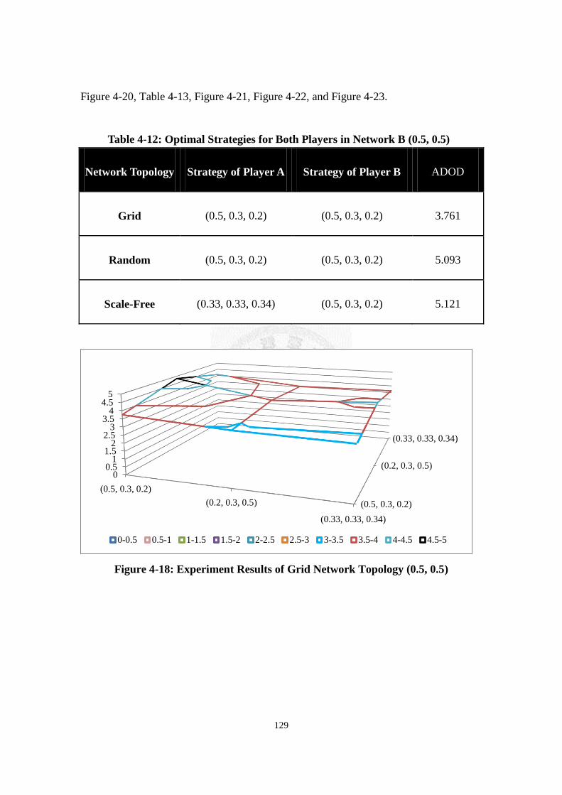
129

Figure 4-20, Table 4-13, Figure 4-21, Figure 4-22, and Figure 4-23.



Grid (0.5, 0.3, 0.2) (0.5, 0.3, 0.2) 3.761

Random (0.5, 0.3, 0.2) (0.5, 0.3, 0.2) 5.093

Scale-Free (0.33, 0.33, 0.34) (0.5, 0.3, 0.2) 5.121

Figure 4-18: Experiment Results of Grid Network Topology (0.5, 0.5)

(0.5, 0.3, 0.2)

(0.2, 0.3, 0.5)

(0.33, 0.33, 0.34)

00.5

11.5

22.5

33.5

44.5

5

(0.5, 0.3, 0.2)

(0.2, 0.3, 0.5)

(0.33, 0.33, 0.34)

0-0.5 0.5-1 1-1.5 1.5-2 2-2.5 2.5-3 3-3.5 3.5-4 4-4.5 4.5-5

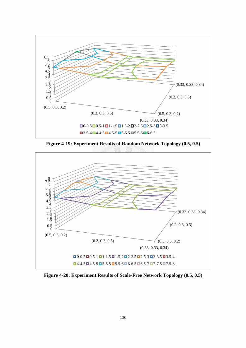
130

Figure 4-19: Experiment Results of Random Network Topology (0.5, 0.5)

Figure 4-20: Experiment Results of Scale-Free Network Topology (0.5, 0.5)

(0.5, 0.3, 0.2)

(0.2, 0.3, 0.5)

(0.33, 0.33, 0.34)

00.5

11.5

22.5

33.5

44.5

55.5

66.5

(0.5, 0.3, 0.2)

(0.2, 0.3, 0.5)

(0.33, 0.33, 0.34)

0-0.5 0.5-1 1-1.5 1.5-2 2-2.5 2.5-3 3-3.5

3.5-4 4-4.5 4.5-5 5-5.5 5.5-6 6-6.5

(0.5, 0.3, 0.2)

(0.2, 0.3, 0.5)

(0.33, 0.33, 0.34)

00.5

11.5

22.5

33.5

44.5

55.5

66.5

77.5

8

(0.5, 0.3, 0.2)

(0.2, 0.3, 0.5)

(0.33, 0.33, 0.34)

0-0.5 0.5-1 1-1.5 1.5-2 2-2.5 2.5-3 3-3.5 3.5-4

4-4.5 4.5-5 5-5.5 5.5-6 6-6.5 6.5-7 7-7.5 7.5-8

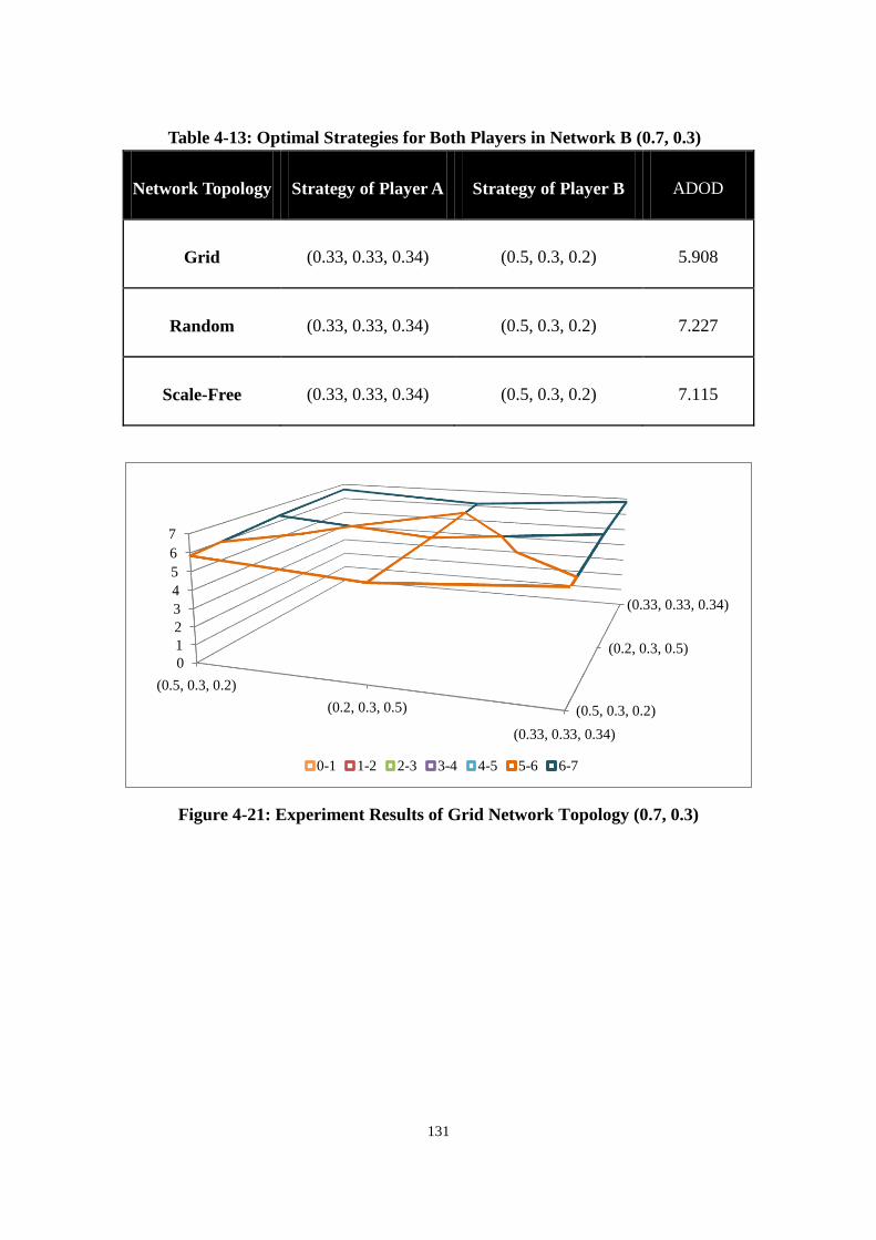
131



Grid (0.33, 0.33, 0.34) (0.5, 0.3, 0.2) 5.908

Random (0.33, 0.33, 0.34) (0.5, 0.3, 0.2) 7.227

Scale-Free (0.33, 0.33, 0.34) (0.5, 0.3, 0.2) 7.115

Figure 4-21: Experiment Results of Grid Network Topology (0.7, 0.3)

(0.5, 0.3, 0.2)

(0.2, 0.3, 0.5)

(0.33, 0.33, 0.34)

0

1

2

3

4

5

6

7

(0.5, 0.3, 0.2)

(0.2, 0.3, 0.5)

(0.33, 0.33, 0.34)

0-1 1-2 2-3 3-4 4-5 5-6 6-7

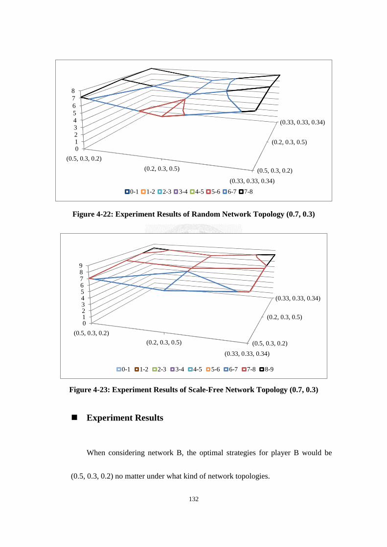
132

Figure 4-22: Experiment Results of Random Network Topology (0.7, 0.3)

Figure 4-23: Experiment Results of Scale-Free Network Topology (0.7, 0.3)

Experiment Results

When considering network B, the optimal strategies for player B would be

(0.5, 0.3, 0.2) no matter under what kind of network topologies.

(0.5, 0.3, 0.2)

(0.2, 0.3, 0.5)

(0.33, 0.33, 0.34)

0123456

7

8

(0.5, 0.3, 0.2)

(0.2, 0.3, 0.5)

(0.33, 0.33, 0.34)

0-1 1-2 2-3 3-4 4-5 5-6 6-7 7-8

(0.5, 0.3, 0.2)

(0.2, 0.3, 0.5)

(0.33, 0.33, 0.34)

0123456789

(0.5, 0.3, 0.2)

(0.2, 0.3, 0.5)

(0.33, 0.33, 0.34)

0-1 1-2 2-3 3-4 4-5 5-6 6-7 7-8 8-9

133


This experiment can verify that the speculation of the previous

experiment is reasonable. In this experiment, when player A’s proportion of

attack resources is getting higher while player B’s proportion of defense

resources is getting lower, player B would like to allocate more total resources

in the first round. In that way, he could have more defense resources to

allocate on proactive defense as early as possible in order to decrease the

probabilities of being compromised.

4.3.1.3 Conclusion

In the series of the experiments, we could make a conclusion that the larger the

proportion of attack to defense resource, the more likely the resource-disadvantaged

player would tend to allocate in the first round in order to increase the proactive defense

resources.

4.3.2 Insufficient Resource Allocation under Different Objectives

In the design of the series of this experiment, we would like to know the

disadvantaged player should allocate his limited resources more on attack or on defense.

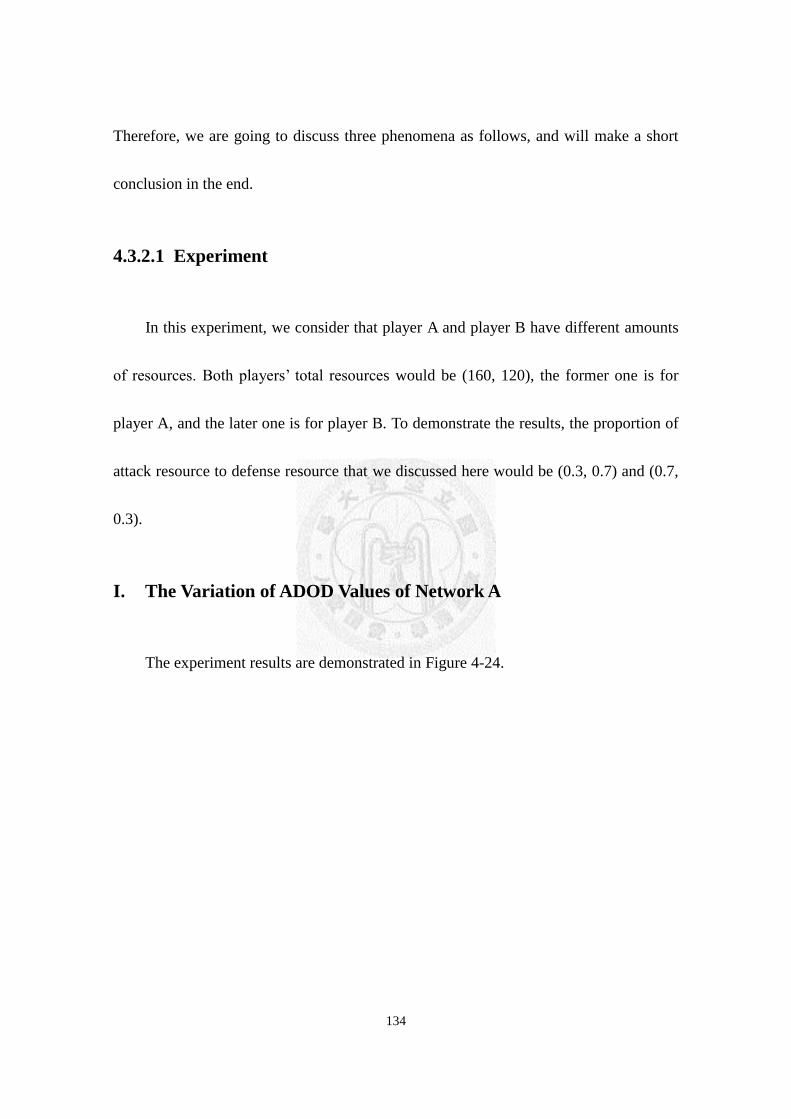
134

Therefore, we are going to discuss three phenomena as follows, and will make a short

conclusion in the end.

4.3.2.1 Experiment




attack resource to defense resource that we discussed here would be (0.3, 0.7) and (0.7,

0.3).


The experiment results are demonstrated in Figure 4-24.

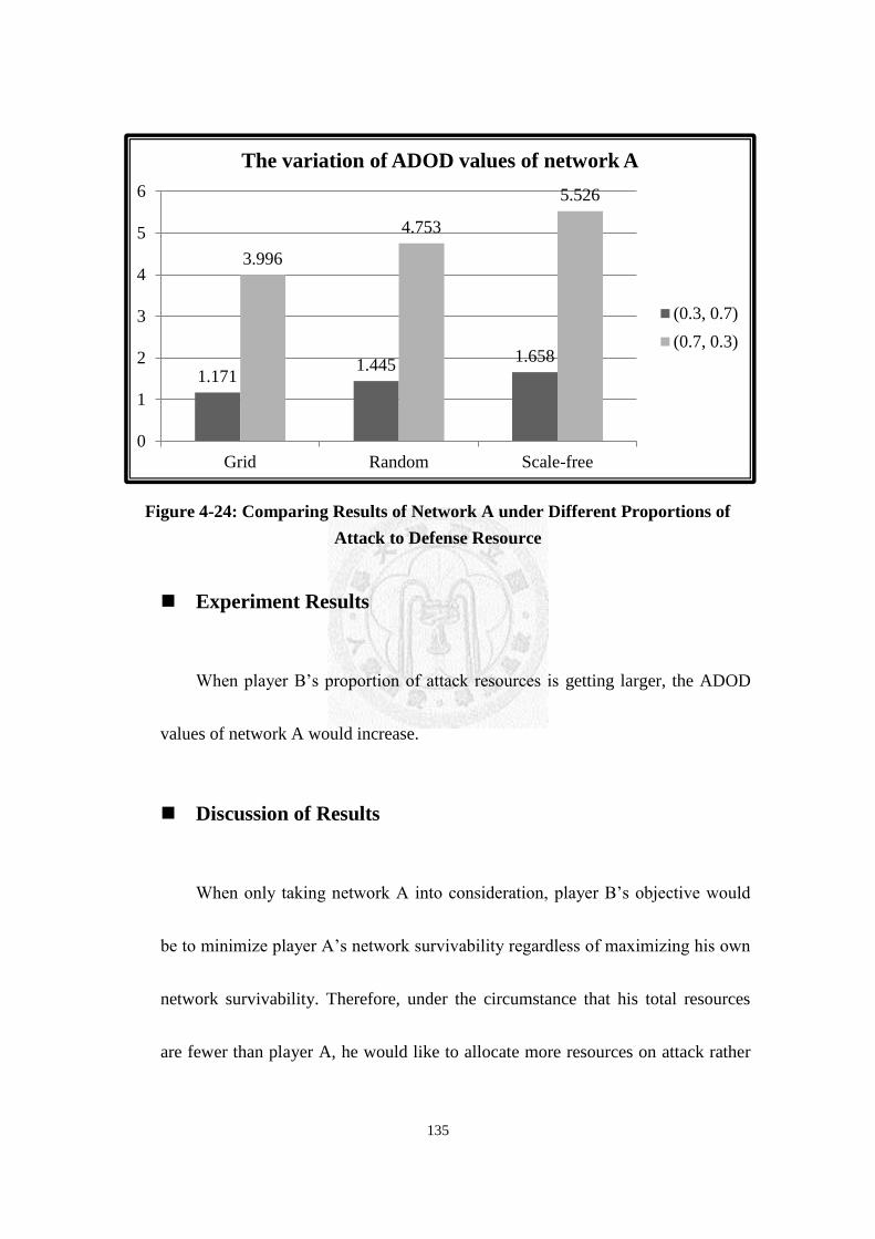
135

Figure 4-24: Comparing Results of Network A under Different Proportions of

Attack to Defense Resource

Experiment Results

When player B’s proportion of attack resources is getting larger, the ADOD

values of network A would increase.


When only taking network A into consideration, player B’s objective would

be to minimize player A’s network survivability regardless of maximizing his own

network survivability. Therefore, under the circumstance that his total resources

are fewer than player A, he would like to allocate more resources on attack rather

1.171 1.445

1.658

3.996

4.753

5.526

0

1

2

3

4

5

6



(0.3, 0.7)

(0.7, 0.3)

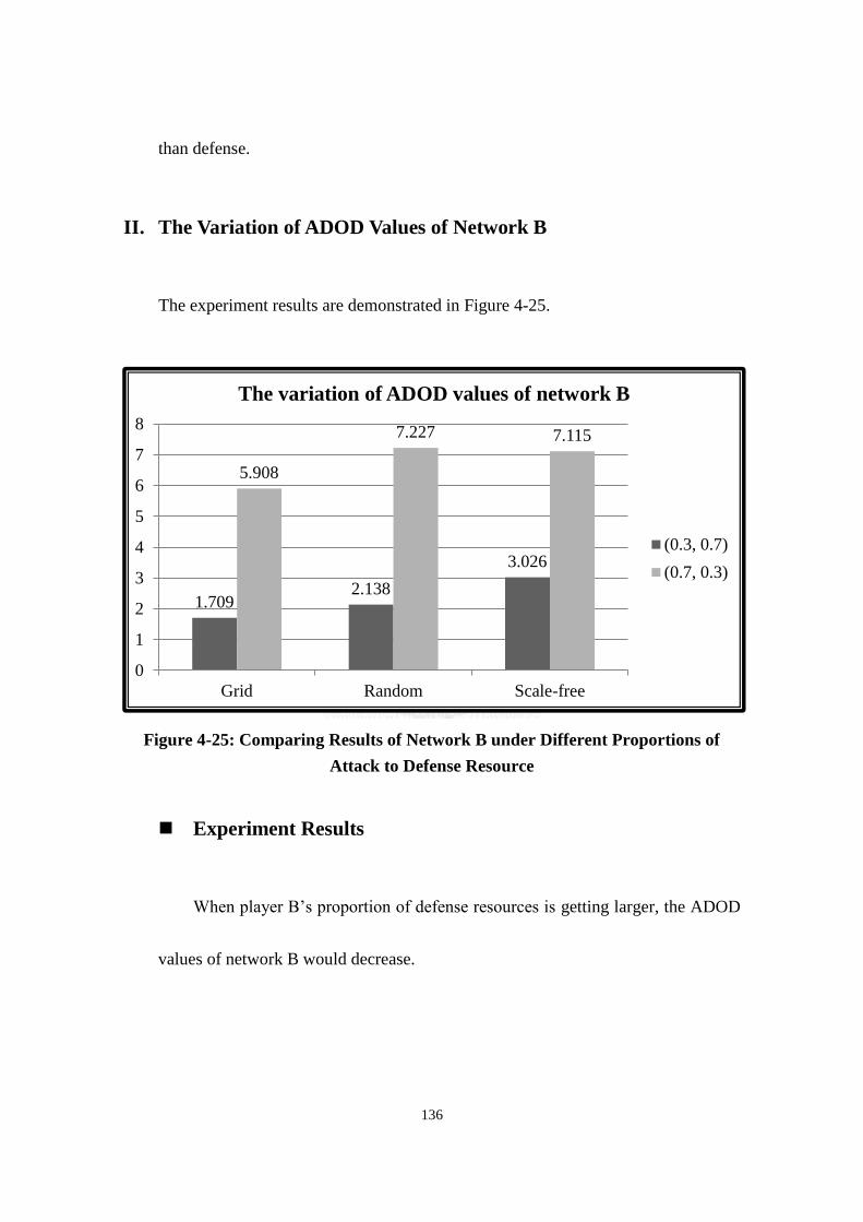
136

than defense.


The experiment results are demonstrated in Figure 4-25.

Figure 4-25: Comparing Results of Network B under Different Proportions of


Experiment Results

When player B’s proportion of defense resources is getting larger, the ADOD

values of network B would decrease.

1.709 2.138

3.026

5.908

7.227 7.115

0

1

2

3

4

5

6

7

8



(0.3, 0.7)

(0.7, 0.3)

137


When only taking network B into consideration, player B’s objective would

be to maximize his network survivability regardless of minimizing player A’s

network survivability. Therefore, under the circumstance that his total resources

are fewer than player A, he would like to allocate more resources on defense rather

than attack.

Under the situation that the resources are fewer than the counterpart’s, the

disadvantaged player would still try his best to allocate his resource to the direction

that might fulfill his objective. In the following experiment, we would like to

further discuss: What if the disadvantaged player wants to achieve both the

objectives of maximizing the counterpart’s damage degree of network and

minimizing his damage degree of network, he would allocate more on defense or

on attack?

III. The Variation of Player B’s Achievement of Objective

In our model, the objective of player B is to maximize the counterpart’s damage

degree of network; meanwhile, to minimize his own damage degree of network.

138

Therefore, in order to observe player B’s achievement of his objective, we would divide

the ADOD value of topology B by the ADOD value of topology A. The ratio is defined

as “Achievement Ratio”. It would be useful to observe some phenomena. The smaller

the achievement ratio indicates that topology A’s ADOD value is much higher than

topology B’s ADOD value, which could be viewed as an implication that player B is

approaching his objective. The experiment results are demonstrated in Figure 4-26.

Figure 4-26: Comparing Results of Player B’s Achievement of Objective under

Different Proportions of Attack to Defense Resource

Experiment Results

When the proportion of attack resources is larger than the proportion of

defense resources, the achievement ratio obtained by dividing the ADOD value of

1.537 1.592

1.925

1.536 1.559

1.372

0

0.5

1

1.5

2


The variation of the achievement ratio of player B

(0.3, 0.7)

(0.7, 0.3)

139

network B by the ADOD value of network A would be smaller.


From player B’s point of view, in order to minimize player A’s network

survivability and to maximize his own network survivability at the same time, he

should allocate more resources on attack since the obtained ratio is smaller in (0.7,

0.3). The phenomenon implies that when he chooses to allocate more resources on

attack, the difference between the ADOD values of topology A and topology B

would be larger, which is more close to player B’s objective.

4.3.2.2 Conclusion

According to the experiment, we could find that different objectives would cause

the disadvantaged player to have different strategies. If he hopes to maximize the

counterpart’s damage degree of network, he should allocate more on attack. On the

other hand, if the objective is to maximize his network survivability, the optimal

strategy for him would become to allocate more resources on defense.

However, the interesting thing is that if the disadvantaged player hopes to achieve

the objective of minimizing the counterpart’s network survivability and maximizing his

140

own network survivability simultaneously, he should choose to allocate more on attack

resource. In this situation, we could view it as “The best defense is attack”.

4.4 Balanced Bipolarity vs. Unbalanced Bipolarity

In previous sections, we have discussed some experiments under the circumstance

of balanced bipolarity or unbalanced bipolarity. In this experiment, we would like to

compare balanced bipolarity with unbalanced bipolarity in the influence on both players’

networks, the situation of both players’ achievement of objectives, and the experiment

results in three different kinds of network topology.

4.4.1 Experiment

To demonstrate the results, there are something needed to be determined. In

balanced bipolarity, both players’ total resources would be (160, 160); in unbalanced

bipolarity, both players’ total resources would be (160, 120), the former one is for player

A, and the later one is for player B. Moreover, the proportion of attack resource to

defense resource that we discussed here would be (0.3, 0.7), (0.5, 0.5), and (0.7, 0.3).

I. The variation of ADOD Values of Network A and Network B

The experiment results are demonstrated in Figure 4-27, Figure 4-28, Figure 4-29,

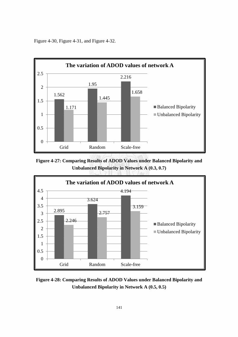
141

Figure 4-30, Figure 4-31, and Figure 4-32.

Figure 4-27: Comparing Results of ADOD Values under Balanced Bipolarity and

Unbalanced Bipolarity in Network A (0.3, 0.7)



1.562

1.95

2.216

1.171

1.445

1.658

0

0.5

1

1.5

2

2.5



Balanced Bipolarity

Unbalanced Bipolarity

2.895

3.624

4.194

2.246

2.757

3.159

0

0.5

1

1.5

2

2.5

3

3.5

4

4.5



Balanced Bipolarity


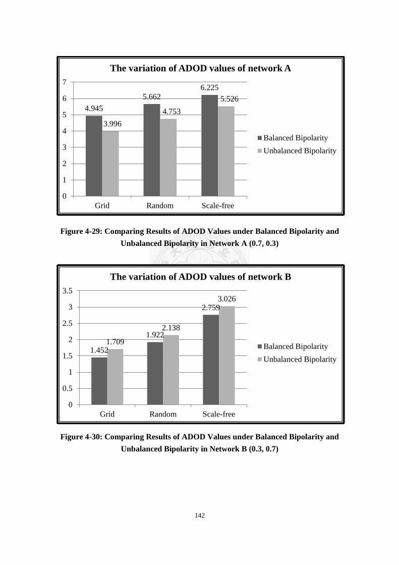
142




Unbalanced Bipolarity in Network B (0.3, 0.7)

4.945

5.662

6.225

3.996

4.753

5.526

0

1

2

3

4

5

6

7



Balanced Bipolarity


1.452

1.922

2.759

1.709

2.138

3.026

0

0.5

1

1.5

2

2.5

3

3.5



Balanced Bipolarity


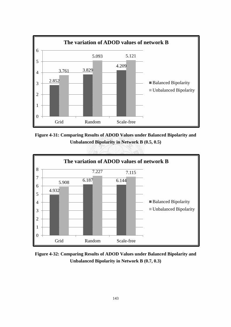
143





2.852

3.829 4.209

3.761

5.093 5.121

0

1

2

3

4

5

6



Balanced Bipolarity


4.932

6.187 6.144 5.908

7.227 7.115

0

1

2

3

4

5

6

7

8



Balanced Bipolarity


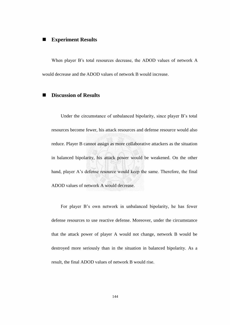
144

Experiment Results

When player B’s total resources decrease, the ADOD values of network A

would decrease and the ADOD values of network B would increase.


Under the circumstance of unbalanced bipolarity, since player B’s total

resources become fewer, his attack resources and defense resource would also

reduce. Player B cannot assign as more collaborative attackers as the situation

in balanced bipolarity, his attack power would be weakened. On the other

hand, player A’s defense resource would keep the same. Therefore, the final

ADOD values of network A would decrease.

For player B’s own network in unbalanced bipolarity, he has fewer

defense resources to use reactive defense. Moreover, under the circumstance

that the attack power of player A would not change, network B would be

destroyed more seriously than in the situation in balanced bipolarity. As a

result, the final ADOD values of network B would rise.

145

II. Player A’s and Player B’s Achievement of Objectives

In our model, the objectives of both players are to maximize the counterpart’s

damage degree of network; meanwhile, to minimize their own damage degree of

network. Therefore, in order to observe one’s achievement of objective, we would

divide the ADOD value of his own network by the ADOD value of the counterpart’s

network. The achievement ratio would be useful to observe some phenomena. The

smaller the achievement ratio indicates that the counterpart’s ADOD value is much

higher than one’s ADOD value, which could be viewed as an implication that the player

is approaching his objective. The experiment results are demonstrated in Figure 4-33,

Figure 4-34, Figure 4-35, Figure 4-36, Figure 4-37, and Figure 4-38.

Figure 4-33: Comparing Results of Player A’s Achievement of Objective under

Balanced Bipolarity and Unbalanced Bipolarity (0.3, 0.7)

1.076 1.028

0.809

0.65 0.628

0.52

0

0.2

0.4

0.6

0.8

1

1.2



Balanced Bipolarity


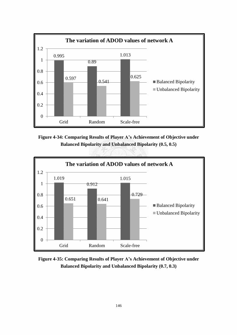
146





0.995

0.89

1.013

0.597 0.541

0.625

0

0.2

0.4

0.6

0.8

1

1.2



Balanced Bipolarity


1.019

0.912

1.015

0.651 0.641 0.729

0

0.2

0.4

0.6

0.8

1

1.2



Balanced Bipolarity


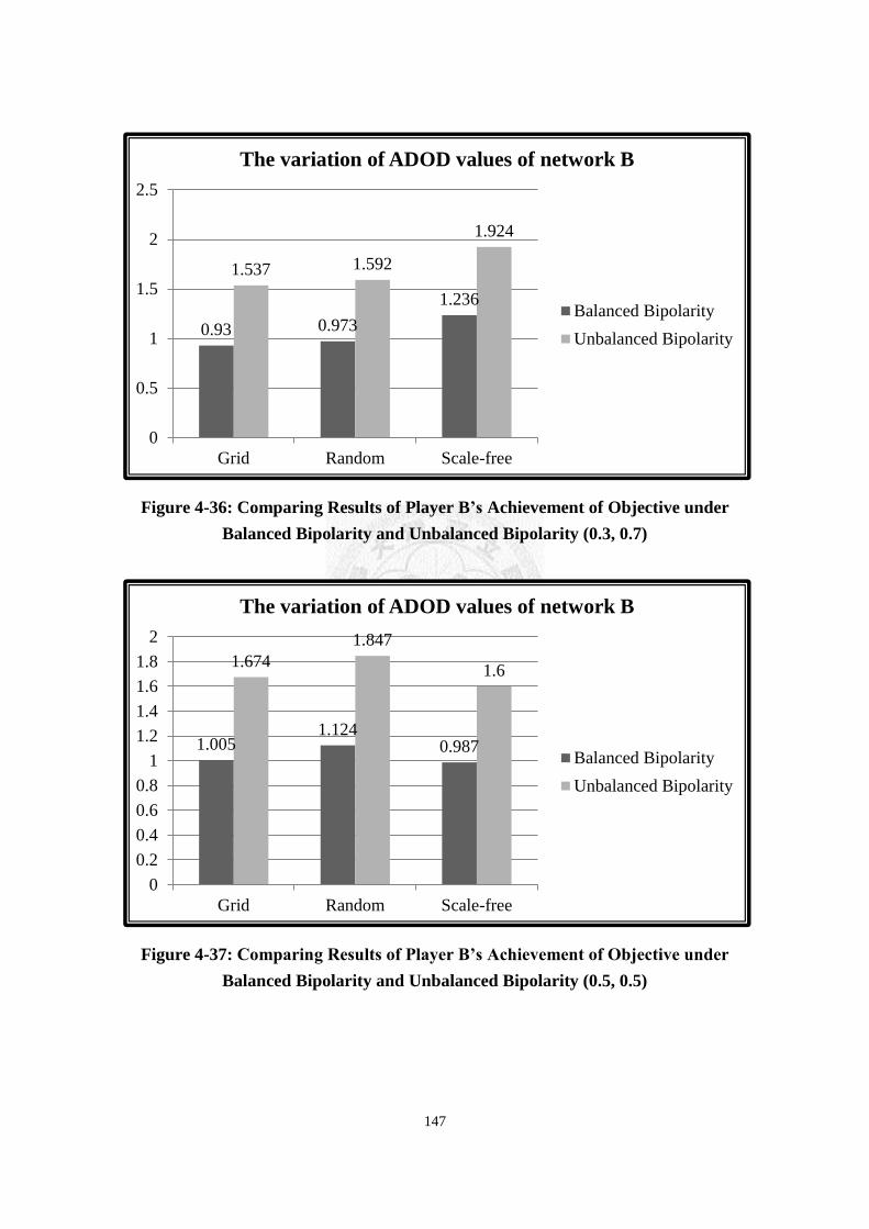
147





0.93 0.973

1.236

1.537 1.592

1.924

0

0.5

1

1.5

2

2.5



Balanced Bipolarity


1.005 1.124

0.987

1.674

1.847

1.6

0

0.2

0.4

0.6

0.8

1

1.2

1.4

1.6

1.8

2



Balanced Bipolarity


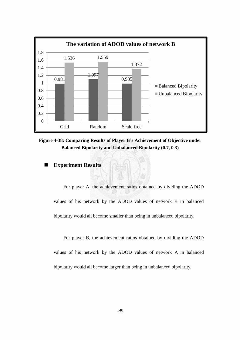
148



Experiment Results

For player A, the achievement ratios obtained by dividing the ADOD

values of his network by the ADOD values of network B in balanced

bipolarity would all become smaller than being in unbalanced bipolarity.

For player B, the achievement ratios obtained by dividing the ADOD

values of his network by the ADOD values of network A in balanced

bipolarity would all become larger than being in unbalanced bipolarity.

0.981 1.097

0.985

1.536 1.559

1.372

0

0.2

0.4

0.6

0.8

1

1.2

1.4

1.6

1.8



Balanced Bipolarity


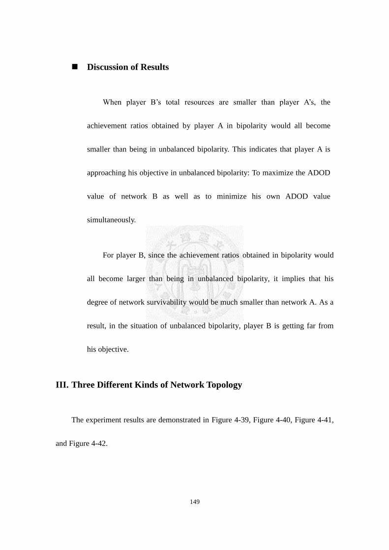
149


When player B’s total resources are smaller than player A’s, the

achievement ratios obtained by player A in bipolarity would all become

smaller than being in unbalanced bipolarity. This indicates that player A is

approaching his objective in unbalanced bipolarity: To maximize the ADOD

value of network B as well as to minimize his own ADOD value

simultaneously.

For player B, since the achievement ratios obtained in bipolarity would

all become larger than being in unbalanced bipolarity, it implies that his

degree of network survivability would be much smaller than network A. As a

result, in the situation of unbalanced bipolarity, player B is getting far from

his objective.

III. Three Different Kinds of Network Topology

The experiment results are demonstrated in Figure 4-39, Figure 4-40, Figure 4-41,

and Figure 4-42.

150

Figure 4-39: Comparing Results of ADOD Values of Network A in Three Different

kinds of Network Topology under Balanced Bipolarity

Figure 4-40: Comparing Results of ADOD Values of Network A in Three Different

kinds of Network Topology under Unbalanced Bipolarity

1.562

2.895

4.945

1.95

3.624

5.662

2.216

4.194

6.225

0

1

2

3

4

5

6

7

(0.3, 0.7) (0.5, 0.5) (0.7, 0.3)


Grid

Random

Scale-Free

1.171

2.246

3.996

1.445

2.757

4.753

1.658

3.159

5.526

0

1

2

3

4

5

6

(0.3, 0.7) (0.5, 0.5) (0.7, 0.3)


Grid

Random

Scale-Free

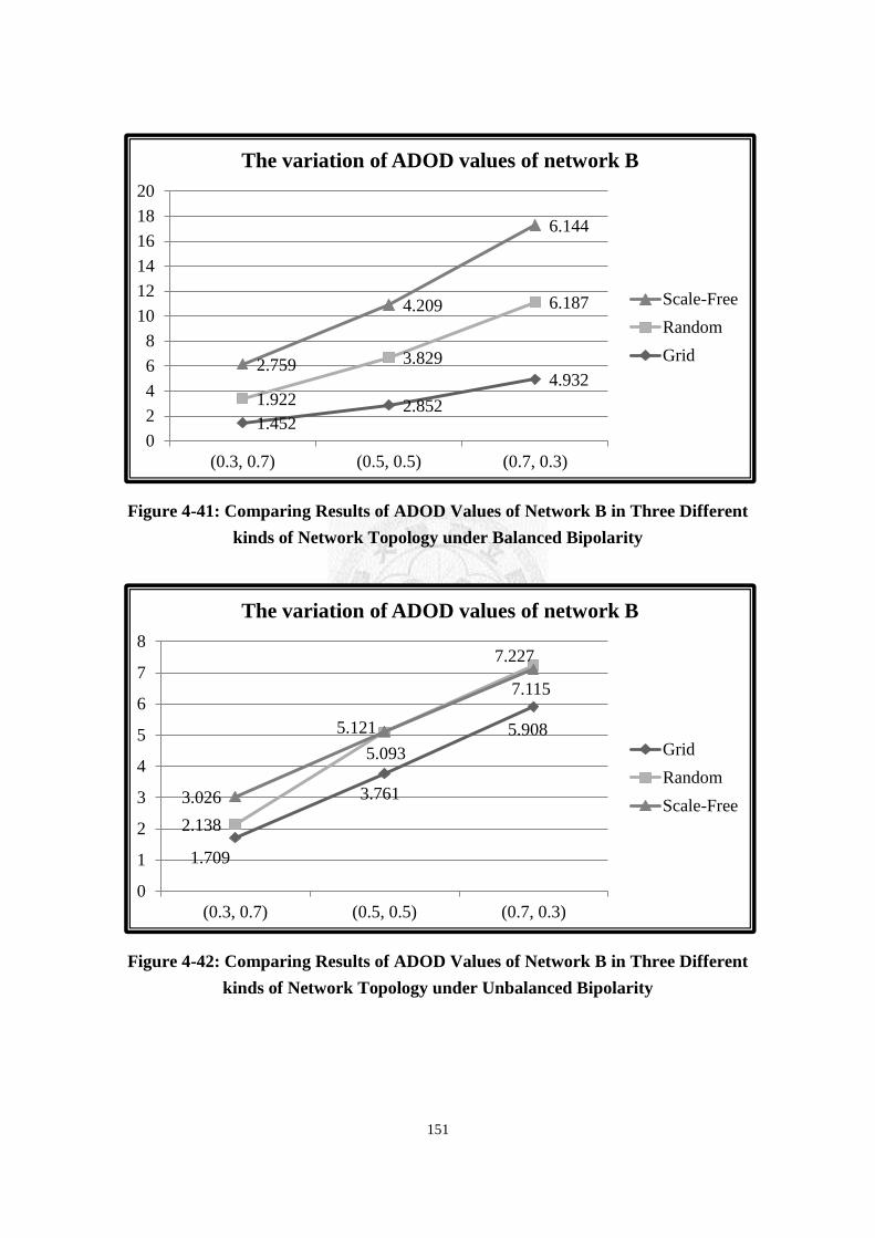
151

Figure 4-41: Comparing Results of ADOD Values of Network B in Three Different

kinds of Network Topology under Balanced Bipolarity

Figure 4-42: Comparing Results of ADOD Values of Network B in Three Different

kinds of Network Topology under Unbalanced Bipolarity

1.452 2.852

4.932 1.922

3.829

6.187

2.759

4.209

6.144

0

2

4

6

8

10

12

14

16

18

20

(0.3, 0.7) (0.5, 0.5) (0.7, 0.3)


Scale-Free

Random

Grid

1.709

3.761

5.908

2.138

5.093

7.227

3.026

5.121

7.115

0

1

2

3

4

5

6

7

8

(0.3, 0.7) (0.5, 0.5) (0.7, 0.3)


Grid

Random

Scale-Free

152

Experiment Results

For both players’ networks, the smallest ADOD values would occur in

grid network topology no matter under what kind of proportions of attack to

defense resource while the largest ADOD values would almost take place in

scale-free network topology except in proportion of (0.7, 0.3) under

unbalanced bipolarity.


This phenomenon indicates that scale-free network topology would be

more vulnerable than grid network topology. The main characteristic of

scale-free network topology is that some important nodes may have more

connections than others and that the network as a whole has a power-law

distribution of the number of links connecting to a node. As a result, if the

important nodes are just located in the combined local views of the players,

the network would have a very big chance to be destroyed seriously.

Comparatively, the structure of grid network topology is more solid under the

same situation.

153

Chapter5 Conclusions and Future Work

5.1 Conclusions

In this paper, we develop a multi-round network attack-defense scenario, and

adopt the mathematical programming approach to solve our problem. In the solution

procedure, the gradient method is used to calculate the Average DOD values and to

find the optimal resource allocation strategy on each node. Then, the game theory is

adopted to determine the optimal percentage resource allocation in each round. As a

result, we transform a complicated problem into a simpler one and finally solved it by

the process of mathematical analysis.

In our research, there are several important contributions which could be

summarized as follows:

1. Considering the Cyberwar between Two Nation-States in the Real World

In the past, the discussion of network security is usually under the scope of an

enterprise or an individual. However, due to political reasons, we nowadays often

154

hear news about the information warfare between two conflicting nation-states in

the real world. Therefore, it is essential to extend the research about the survivability

of a network from an individual or an enterprise level to a nation-state level. In our

research, we model two players as two conflicting nation-states in a cyberwar; and

in the end, the optimal resource allocation for both nation-states is attained, which

would be a critical contribution.

2. Attack-Defense Dual-Role

In the past, we often consider an attacker and a defender in an attack-defense

model. On one hand, the network defender would protect his network; on the other

hand, the cyber attacker would try to destruct the network. However, from the point

of view of a nation-state, in order to protect his critical infrastructures or territory

from other nation-states, he would allocate much defense resource on his network;

in addition, in order to expand his national power (or other political concerns), he

might intrude into other nation-states by military power. Apparently, it is

insufficient to consider only attack or only defend one at a time in our research. As

a result, we consider each player in our model could defend and attack at the same

time, which is called attack-defense dual-role. This would be a great contribution,

155

since this characteristic is based on the nature of a nation-state in the real world.

3. Collaborative Attacks

Instead of considering only one attacker, we consider a group of attackers

simultaneously mount an attack in our model. Moreover, each collaborative attacker

has his own attack power which would also be influenced by the other collaborative

attackers and the leader. The final synergy might be positive or unfortunately

negative, which means we not only consider the “1+1>2” situation but also the

“1+1<2” phenomenon. Involving the concept of collaborative attacks in our model

would be an important contribution, since it makes us further consider the diversity

of different attackers’ expertise, which is necessary and realistic in a cyberwar.

4. Multi-Round Attack-Defense

One of our objectives in this research is to extend the attack-defense scenario to

multiple rounds. Therefore, our experiments are demonstrated under the scope of

three rounds. Actually, the problem is complicated enough when considering three

rounds. The time complexity is O(43V

WV2) (Where V is the node number in the

network, and W is the number of the O-D pair).

156

5. Guidelines for the Decision-Making of a Nation-State

The problem that we consider in this paper and some phenomena observed

from the experiment results might help the security experts of a nation-state to make

an optimal resource allocation on defense and attack and further to enhance their

national security in a cyberwar.

If knowing complete information of the counterpart’s, the nation-state should

allocate more total resources in the first stage when the proportion of attack

and defense resources on his own network and the counterpart’s are different,

but uniformly allocate total resources to each round when attack and defense

resources are the same.

If knowing incomplete information of the counterpart’s, the nation-state

should uniformly allocate in three stages when available attack resources are

more. Moreover, if both attack and defense resources allocated on the

network are the same, the nation-state should allocate more total resources in

the first stage. Finally, when the available attack resources are more, to

allocate in the first round or uniformly allocate in each round depends on the

nation-state’s objective.

157

To strike preventively would always help a nation-state to enhance his degree

of network survivability (Further experiment is in Appendix).

If a nation-sate is the resource-disadvantaged, he should allocate more on

attack since this would make him minimize the counterpart’s network

survivability while maximize his own network survivability simultaneously.

Furthermore, “The best defense is attack” not only holds for the

resource-disadvantaged, but also holds in the situation that both nation-sates

have the same amount of resources (Further experiment is in Appendix).

5.2 Future Work

The following are some issues that can be further studied:

Collaborative Defense

In our model, we only consider collaborative attacks. However, from the point

of view of a nation-state, there must exist various information security experts not

only specialize in attack but also specialize in defense. In [34], the author said that

in order to counter collaborative attacks, we might need collaborative defense.

Therefore, in the future work, we could consider some of the experts might form a

158

group of collaborative attackers while some might form a group of collaborative

defenders.

Multiple Players (Nation-States)

In this paper, we propose a framework to model two conflicting nation-states

in the cyberwar. Nevertheless, the political tensions between nation-states,

especially those super power nation-states, are often heard from daily news. To

further simulate the circumstances in the real world, more players (nation-states)

to join a battle might be necessary to be considered in the future work.

Now we take three players for instance. On one hand, the three players could

attack each other individually. On the other hand, two of them could also form an

alliance to mount the other one. In this way, the combinations of the players

would be more complicated to consider, which enhances the richness of the

original problem.

Anticipatory Strategy

In real world, under some circumstances, a nation-state would like to strike

first. We have included the concept of preventive strike in our research.

159

Nevertheless, according to [55], aside from preventive strike, preemptive strike

also belongs to this kind of first-strike strategy. The authors used the term

“anticipatory attack” to refer to the broader category that includes both types of

strategies. Both of them are offensive strategies carried out for defensive reasons,

based on the belief that an enemy attack is (or may be) inevitable, and it would

be better to fight on one’s own terms. Furthermore, “the degree of certainty that

the adversary will strike if the anticipatory attack is not launched,” and “the

first-strike advantage expected from carrying out the anticipatory attack

compared to allowing the opponent to attack on its own terms” are two

fundamental strategic variables determining whether preemptive or preventive

attack should take.

Therefore, in the future work, it would be meaningful to consider

preemptive strike strategy as well and to include the two strategic variables

aforementioned in the model to further consider which strategy might be better.

Unique Attack Strategy for each Collaborative Attacker

In our model, each collaborative attacker could have different attack power

over nodes. This could be viewed as a distinctive attribute for each collaborative

160

attacker. Furthermore, it would be interesting to consider that each attacker has

their own attack strategy. For instance, some may specialize in taking PS strategy;

while some may especially good at exploring unknown vulnerabilities. That is,

when the collaborative attacker who is skilled in exploring unknown vulnerabilities

is assigned to join the battle this round, the result of exploration would be better

this round. Or if the collaborative attacker who excels at taking PS strategy is

assigned in the next round, then the player could take PS strategy in that round.

The Weight of Link in Calculating DOD

The link vulnerability explicitly accounts for the flow on the disrupted link

and the availability of alternate paths. Link is a component of O-D pairs, and a link

may belong to many O-D pairs. When the link is disrupted, it will need other

alternative paths to accommodate the affected flow. Therefore, the importance of a

link would affect the connectivity of an O-D pair, and finally influence the network

survivability. As a result, the weight of link should be taken into consideration

when calculating the DOD metric.

161

N-Round Attack-Defense

The complexity of our mathematical problem would increase in an

exponential way when considering one round more; therefore, the problem is

quite difficult to solve. We would always like to know if there exists a steady

condition of the network survivability, which means to have one more round or

not might not influence the network survivability too much any longer. As a result,

in order to verify whether the conjecture is right or not, it is necessary to extend

the number of attack-defense rounds as huge as possible.

Because of the diversity of the attack-defense problem, there are multiple

different kinds of issues that could be discussed. Therefore, more and more issues

would be extended to reflect reality in the future.

163

References

[1] SAINT, “Integrated Network Vulnerability Scanning and Penetration Testing,”

SAINT, 2009.

[2] IBM Internet Security Systems X-Force research and development team,

“X-Force 2011 Mid-Year Trend and Risk Report,” IBM, September 2011.

[3] R. Robert, “CSI Computer Crime and Security Survey 2010/2011,” Computer

Security Institute, 2011.

[4] Symantec, “2011 State of Security Survey,” Symantec Corporation, 2011.

[5] R.A. Clarke, “Cyber War,” HarperCollins, 2010,

http://en.wikipedia.org/wiki/Cyberwarfare.

[6] McAfee, “Advanced Persistent Threats,” McAfee, 2010.

[7] Jonathan Fildes, “Stuxnet Worm Targeted High-Value Iranian Assets,” BBC news,

September 2010, http://www.bbc.com/news/technology-11388018.

[8] D.E. Sanger, “Obama Order Sped Up Wave of Cyber Attacks Against Iran,” New

York Times, June 2012,

http://www.nytimes.com/2012/06/01/world/middleeast/obama-ordered-wave-of-c

yberattacks-against-iran.html?_r=2.

[9] Kevin Fogarty, “Iran official threatens retaliation for Stuxnet,” IT World, April,

http://en.wikipedia.org/wiki/Cyberwarfare

http://www.bbc.com/news/technology-11388018

http://www.nytimes.com/2012/06/01/world/middleeast/obama-ordered-wave-of-cyberattacks-against-iran.html?_r=2

http://www.nytimes.com/2012/06/01/world/middleeast/obama-ordered-wave-of-cyberattacks-against-iran.html?_r=2

164

2011.

[10] SANS, “A Detailed Analysis of an Advanced Persistent Threat Malware,” SANS,

October, 2011.

[11] “Terms and Definitions Related to Quality of Service, Availability, and Reliability,”

CCITT Fascicle III. 1Rec. G. 106, 1984.

[12] V.R. Westmark, “A Definition for Information System Survivability,” System

Sciences, Proceedings of the 37th Annual Hawaii International Conference on,

January 2004.

[13] R.J. Ellison, D.A. Fisher, R.C. Linger, H.F. Lipson, T. Longstaff, and N.R. Mead,

“Survivable Network Systems: An Emerging Discipline,” Technical Report

CMU/SEI-97-TR-013, November 1997.

[14] W. Jiang, B.X. Fang, H.l. Zhang, and Z.H. Tian, “A Game Theoretic Method for

Decision and Analysis of the Optimal Active Defense Strategy,” International

Conference on Computational Intelligence and Security, 2007.

[15] W. Jiang, B.X. Fang, H.l. Zhang, and Z.H. Tian, “Optimal Network Security

Strengthening Using Attack-Defense Game Model,” Sixth International

Conference on Information Technology: New Generations, 2009.

[16] Y.S. Lin, P.H. Tsang, C.H. Chen, C.L. Tseng, and Y.L. Lin, “Evaluation of

165

Network Robustness for Given Defense Resource Allocation Strategies,”

Proceedings of the First International Conference on Availability, Reliability and

Security, 2006.

[17] F.Y.S. Lin, H.H. Yen, P.Y. Chen, and Y.F. Wen, “Evaluation of Network

Survivability Considering Degree of Separation,” Hybrid Artificial Intelligence

Systems, 2011.

[18] F.Y.S. Lin, P.Y. Chen, Q.T. Chen, “Resource Allocation Strategies to Maximize

Network Survivability Considering of Average DOD”, Advances in Intelligent

and Soft Computing, Vol. 151, pp. 751-758, 2012.

[19] S. Skaperdas, “Contest Success Functions,” Economic Theory, 1996.

[20] K. Kark, J. Penn, and A. Dill, “2008 CISO Priorities: The Right Objectives but

The Wrong Focus,” Le Magazine de la Sécurité Informatique, April 2009.

[21] J.P. Pironti, “Key Elements of an Information Security Program,” Information

Systems Control Journal, vol. 1, 2005.

[22] A.Barth, B. Rubinstein, M. Sundararajan, J.C. Mitchell, D. Song, and P.L. Bartlett,

“A Learning-Based Approach to Reactive Security,” Proceeding of the Fourteenth

International Conference on Financial Cryptography and Data Security, 2010.

[23] Y. Xiang, W. Zhou, and M. Chowdhury, “A Survey of Active and Passive Defence

166

Mechanisms against DDoS Attacks,” Technical Report, TR C04/02, School of

Information Technology, Deakin University, Australia, 2004.

[24] G. Levitin, K. Hausken, and H. Ben Haim, “Active and Passive Defense against

Multiple Attack Facilities,” International Game Theory Review, 2010.

[25] G. Levitin and K. Hausken, “Preventive Strike vs. False Targets and Protection in

Defense Strategy,” Reliability Engineering & System Safety, vol. 96, issue 8, pp.

912–924, 2011.

[26] G. Levitin and K. Hausken, “Preventive Strike vs. Protection in Defense Strategy,”

Military Operations Research, vol. 15(3), pp. 5-15, 2010.

[27] G. Levitin and K. Hausken, “Shield vs. Sword Resource Distribution in K-round

Duels,” Central European Journal of Operations Research, vol. 8, pp. 1-15, June

2010.

[28] V. Kroening, “Prevention or Preemption? Towards a Clarification of Terminology,”

Commonwealth Institute Project on Defense Alternatives Guest Commentary,

2003.

[29] T. Sauer, “The Preventive and Pre-Emptive Use of Force,” Ethical Perspectives,

vol. 11, no. 2-3, pp. 130-142, 2004.

[30] P.S. Ford, “Israel's Attack on Osiraq: A Model for Future Preventive Strikes,”

167

INSS Occasional Paper 59, USAF Institute for National Security Studies, USAF

Academy, Colorado, pp. 15, July 2005.

[31] B. Bhargava, Y. Zhang, N. Idika, L. Lilien, and M. Azarmi, “Collaborative

Attacks in WiMAX Networks,” Security and Communication Networks, vol. 2(5),

pp. 373-391, 2009.

[32] T. Gong and B. Bhargava, “Immunizing Mobile Ad Hoc Networks against

Collaborative Attacks Using Cooperative Immune Model,” Security and

Communication Networks, 2011. (Under Review)

[33] X. Li and S. Xu, “A Stochastic Modeling of Coordinated Internal and External

Attacks,” Technical Report, 2007.

[34] S. Xu, “Collaborative Attack vs. Collaborative Defense,” Lecture Notes of the

Institute for Computer Sciences, Social Informatics and Telecommunications

Engineering, vol. 10(2), pp. 217-228, 2009.

[35] Websense, “Advanced Persistent Threats and Other Advanced Attacks: Threat

Analysis and Defense Strategies for SMB, Mid-size, and Enterprise

Organizations,” Websense, September 2011.

[36] A. Juels and T.F. Yen, “Sherlock Holmes and the Case of the Advanced Persistent

Threat,” RSA Laboratories, Cambridge, MA, USA, April 2012.

168

[37] Mandiant, “M-Trends, the Advanced Persistent Threat,” Mandiant, January 2010.

[38] Command Five Pty Ltd, “Advanced Persistent Threats: A Decade in Review,”

Command Five Pty Ltd, June 2011.

[39] Jason Andress, “Advanced Persistent Threat: Attacker Sophistication Continues to

Grow,” ISSA Journal, June 2011.

[40] M.S. Deutsch and R.R. Willis, “Software Quality Engineering: A Total Technical

and Management Approach,” Englewood Cliffs, NJ: Prentice-Hall, 1988.

[41] U.S. Department of Commerce, National Telecommunications and Information

Administration, Institute for Telecommunications Services, Federal Standard

1037C.

[42] P.G. Neumann, “Practical Architectures for Survivable Systems and Networks,”

Technical Report, Computer Science Laboratory, SRI International, CA, 2000.

[43] J. Knight and K. Sullivan, “On the Definition of Survivability,” Department of

Computer Science, University of Virginia, Tech. Rep. CS-00- 33, December 2000.

[44] S.D. Moitra and S.L. Konda, “A Simulation Model for Managing Survivability of

Networked Information Systems,” SEI, December 2000.

[45] S. Jha, J.M. Wing, “Survivability Analysis of Networked Systems,” Proceedings

of the Twenty-Third International Conference on Software Engineering, pp.

169

872-874 2001.

[46] H. Kerivin and A.R. Mahjoub, “Design of Survivable Networks: A survey.

Networks,” vol. 46(1), pp.1–21, 2005.

[47] B. Bassiri and S.S. Heydari,“Network Survivability in Large-Scale Regional

Failure Scenarios,” Proceedings of the Second Canadian Conference on

Computer Science and Software Engineering, Montreal, Quebec, Canada, pp.

83–87, 2009.

[48] P.E. Heegaard and K.S. Trivedi, “Network Survivability Modeling,” Computer

Networks, vol. 53(8), pp. 1215-1234, 2009.

[49] F. Xing and W. Wang, “On the Survivability of Wireless Ad Hoc Networks with

Node Misbehaviors and Failures,” IEEE Transactions on Dependable and Secure

Computing, vol. 7, no. 3, pp. 284-299, 2010.

[50] D. Chen, S. Garg, and K.S. Trivedi, “Network Survivability Performance

Evaluation: A Quantitative Approach with Applications in Wireless Ad-Hoc

Networks,” ACM International Workshop on Modeling, Analysis and Simulation

of Wireless and Mobile System, ACM, Atlanta, GA, September 2002.

[51] G. Zhao, H. Wang, and J. Wang, “A Novel Formal Analysis Method of Network

Survivability Based on Stochastic Process Algebra,” Tsinghua Science Technology,

170

vol. 12, pp. 175-179, July 2007.

[52] H. Hassoun, “Fundamentals of Artificial Neural Networks,” MIT Press, 1995.

[53] S. Roy, C. Ellis, S. Shiva, D. Dasgupta, V. Shandilya, and Q. Wu, “A Survey of

Game Theory as Applied to Network Security”, 43rd Hawaii International

Conference on System Sciences, January 2010.

[54] G. Owen, “Game Theory, 3rded,” Academic Press, 2001.

[55] K.P. Mueller, J.J. Castillo, F.E. Morgan, N. Pegahi, and B. Rosen, “Striking First:

Preemptive and Preventive Attack in U.S. National Security Policy,” RAND

Corporation, 2016.

[56] J.J. Mearsheimer, “The Tragedy of Great Power Politics,” New York: W. W.

Norton & Company, 2001.

[57] Y.K. Wang, “Offensive Realism and the Rise of China,” Issues & Studies, vol. 40,

no. 1, pp. 173-201, March 2004.

[58] P. Toft, “John J. Mearsheimer: an offensive realist between geopolitics and power,”

Journal of International Relations and Development, vol 8, pp. 383-386,

December 2005.

[59] N.D. Arora, “Political Science for Civil Services Main Examination,” Tata

McGraw-Hill, 2010.

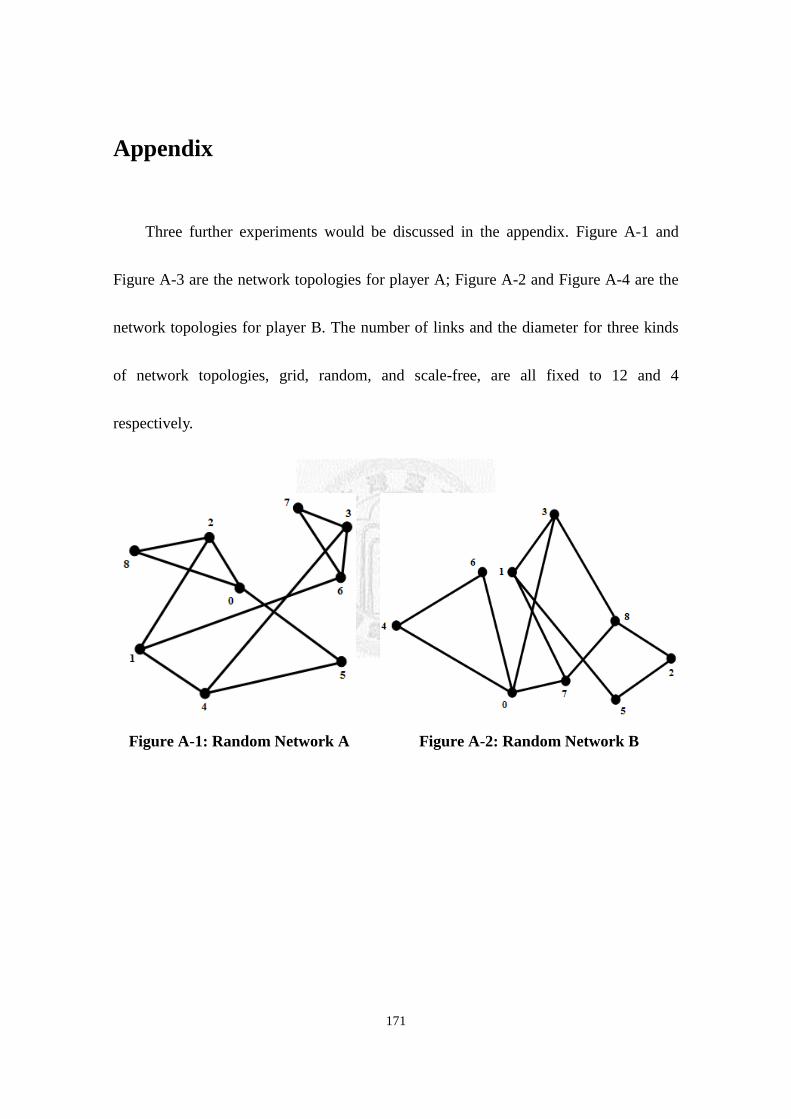
171

Appendix

Three further experiments would be discussed in the appendix. Figure A-1 and

Figure A-3 are the network topologies for player A; Figure A-2 and Figure A-4 are the

network topologies for player B. The number of links and the diameter for three kinds

of network topologies, grid, random, and scale-free, are all fixed to 12 and 4

respectively.

Figure A-1: Random Network A

Figure A-2: Random Network B

172

Figure A-3: Scale-Free Network A Figure A-4: Scale-Free Network B

The parameters used in the following experiments are shown in Table A-1.

Table A-1: Experiment Parameters Settings

Parameters Value

Network Topology

1. Random for player A (In Figure A-1)

2. Random for player B (In Figure A-2)

3. Scale Free for player A (In Figure A-3)

4. Scale Free for player B (In Figure A-4)

Contest intensity (m) 1

The number of rounds 3

The number of nodes 9

The number of links 12

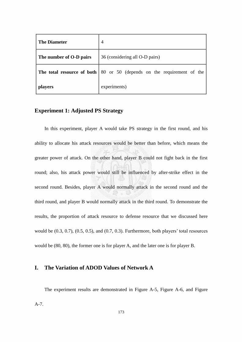
173

The Diameter 4

The number of O-D pairs 36 (considering all O-D pairs)

The total resource of both

players

80 or 50 (depends on the requirement of the

experiments)

Experiment 1: Adjusted PS Strategy

In this experiment, player A would take PS strategy in the first round, and his

ability to allocate his attack resources would be better than before, which means the

greater power of attack. On the other hand, player B could not fight back in the first

round; also, his attack power would still be influenced by after-strike effect in the

second round. Besides, player A would normally attack in the second round and the

third round, and player B would normally attack in the third round. To demonstrate the

results, the proportion of attack resource to defense resource that we discussed here

would be (0.3, 0.7), (0.5, 0.5), and (0.7, 0.3). Furthermore, both players’ total resources

would be (80, 80), the former one is for player A, and the later one is for player B.


The experiment results are demonstrated in Figure A-5, Figure A-6, and Figure

A-7.

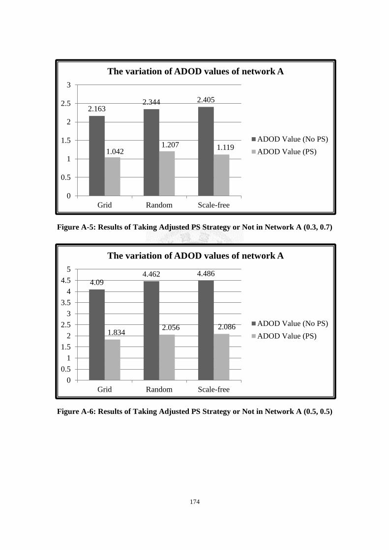
174

Figure A-5: Results of Taking Adjusted PS Strategy or Not in Network A (0.3, 0.7)

Figure A-6: Results of Taking Adjusted PS Strategy or Not in Network A (0.5, 0.5)

2.163 2.344 2.405

1.042 1.207 1.119

0

0.5

1

1.5

2

2.5

3



ADOD Value (No PS)

ADOD Value (PS)

4.09 4.462 4.486

1.834 2.056 2.086

0

0.5

1

1.5

2

2.5

3

3.5

4

4.5

5



ADOD Value (No PS)

ADOD Value (PS)

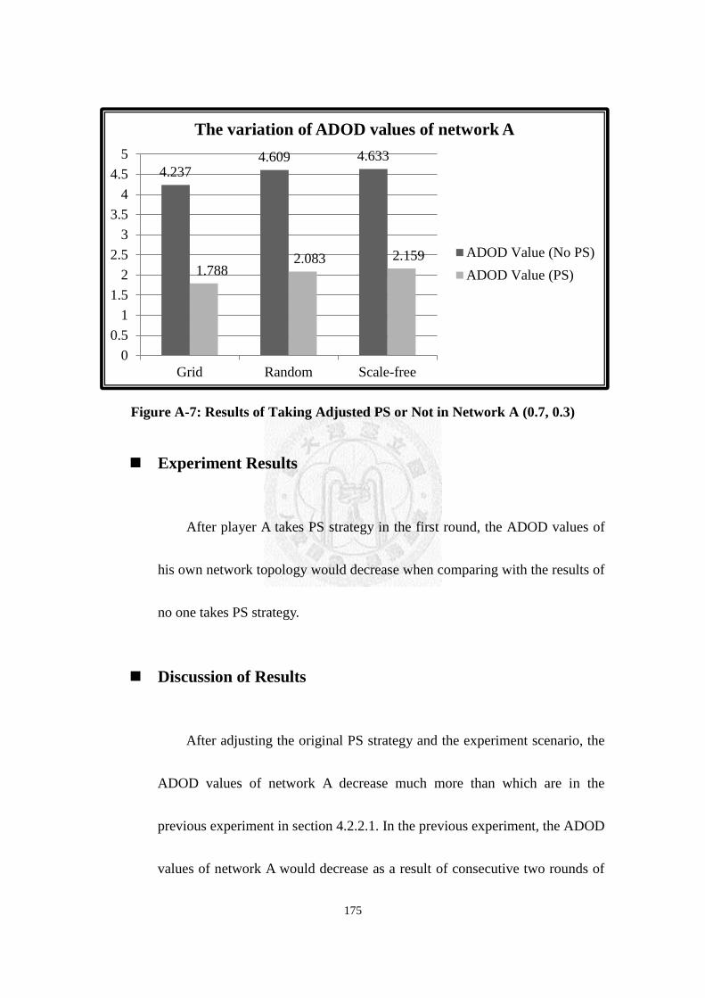
175

Figure A-7: Results of Taking Adjusted PS or Not in Network A (0.7, 0.3)

Experiment Results

After player A takes PS strategy in the first round, the ADOD values of

his own network topology would decrease when comparing with the results of

no one takes PS strategy.


After adjusting the original PS strategy and the experiment scenario, the

ADOD values of network A decrease much more than which are in the

previous experiment in section 4.2.2.1. In the previous experiment, the ADOD

values of network A would decrease as a result of consecutive two rounds of

4.237 4.609 4.633

1.788 2.083 2.159

0

0.5

1

1.5

2

2.5

3

3.5

4

4.5

5



ADOD Value (No PS)

ADOD Value (PS)

176

after-strike effect, which influences player B’s retaliation ability in the second

and the third round. However, in this experiment, not only the influence of

after-strike effect in the second round but also player B is limited not to fight

back in the first round that together largely decrease the ADOD values of

network A. Since player B could not attack in the first round, network A is

remained complete in the initial of the second round. Therefore, the final

network survivability increases much more than that is in the previous

experiment.

II. The Comparison between Previous and Adjusted PS of Network A

The following three charts of experiment results illustrate the percentage of

decrease of ADOD values of network A after taking previous PS strategy or after

taking adjusting PS strategy. The number of the above curve in any one of the

three charts is attained by dividing the difference of ADOD value after taking

previous PS strategy minus not taking PS strategy by the ADOD value of not

taking PS strategy in the original experiment in section 4.2.2.1:

The above Number on the Curve =ADOD(Previous PS Strategy)-ADOD(No PS)

ADOD(No PS) .

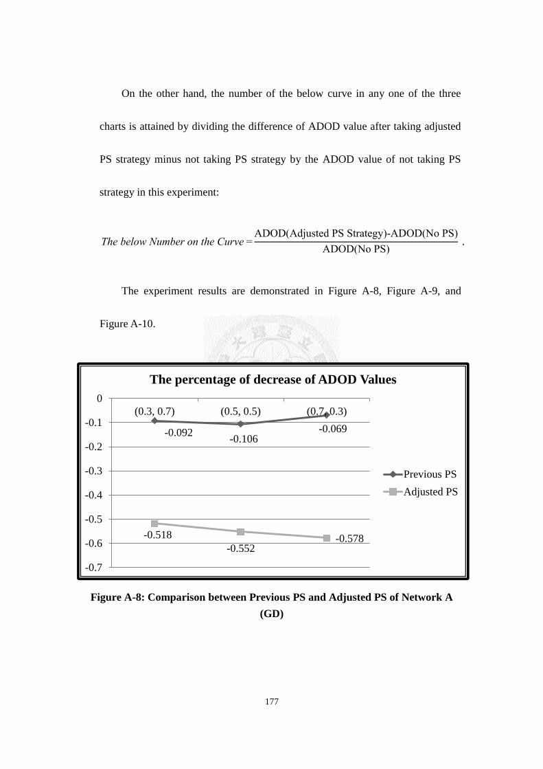
177

On the other hand, the number of the below curve in any one of the three

charts is attained by dividing the difference of ADOD value after taking adjusted

PS strategy minus not taking PS strategy by the ADOD value of not taking PS

strategy in this experiment:

The below Number on the Curve =ADOD(Adjusted PS Strategy)-ADOD(No PS)

ADOD(No PS) .

The experiment results are demonstrated in Figure A-8, Figure A-9, and

Figure A-10.

Figure A-8: Comparison between Previous PS and Adjusted PS of Network A

(GD)

-0.092 -0.106

-0.069

-0.518

-0.552 -0.578

-0.7

-0.6

-0.5

-0.4

-0.3

-0.2

-0.1

0

(0.3, 0.7) (0.5, 0.5) (0.7, 0.3)

The percentage of decrease of ADOD Values

Previous PS

Adjusted PS

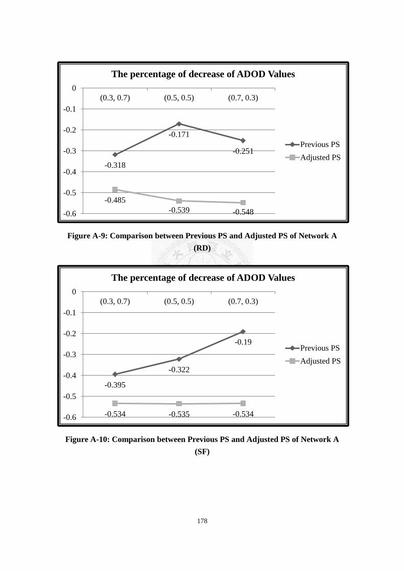
178


(RD)


(SF)

-0.318

-0.171

-0.251

-0.485

-0.539 -0.548 -0.6

-0.5

-0.4

-0.3

-0.2

-0.1

0

(0.3, 0.7) (0.5, 0.5) (0.7, 0.3)


Previous PS

Adjusted PS

-0.395

-0.322

-0.19

-0.534 -0.535 -0.534 -0.6

-0.5

-0.4

-0.3

-0.2

-0.1

0

(0.3, 0.7) (0.5, 0.5) (0.7, 0.3)


Previous PS

Adjusted PS

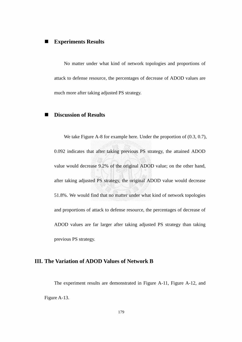
179

Experiments Results

No matter under what kind of network topologies and proportions of

attack to defense resource, the percentages of decrease of ADOD values are

much more after taking adjusted PS strategy.


We take Figure A-8 for example here. Under the proportion of (0.3, 0.7),

0.092 indicates that after taking previous PS strategy, the attained ADOD

value would decrease 9.2% of the original ADOD value; on the other hand,

after taking adjusted PS strategy, the original ADOD value would decrease

51.8%. We would find that no matter under what kind of network topologies

and proportions of attack to defense resource, the percentages of decrease of

ADOD values are far larger after taking adjusted PS strategy than taking

previous PS strategy.

III. The Variation of ADOD Values of Network B


Figure A-13.

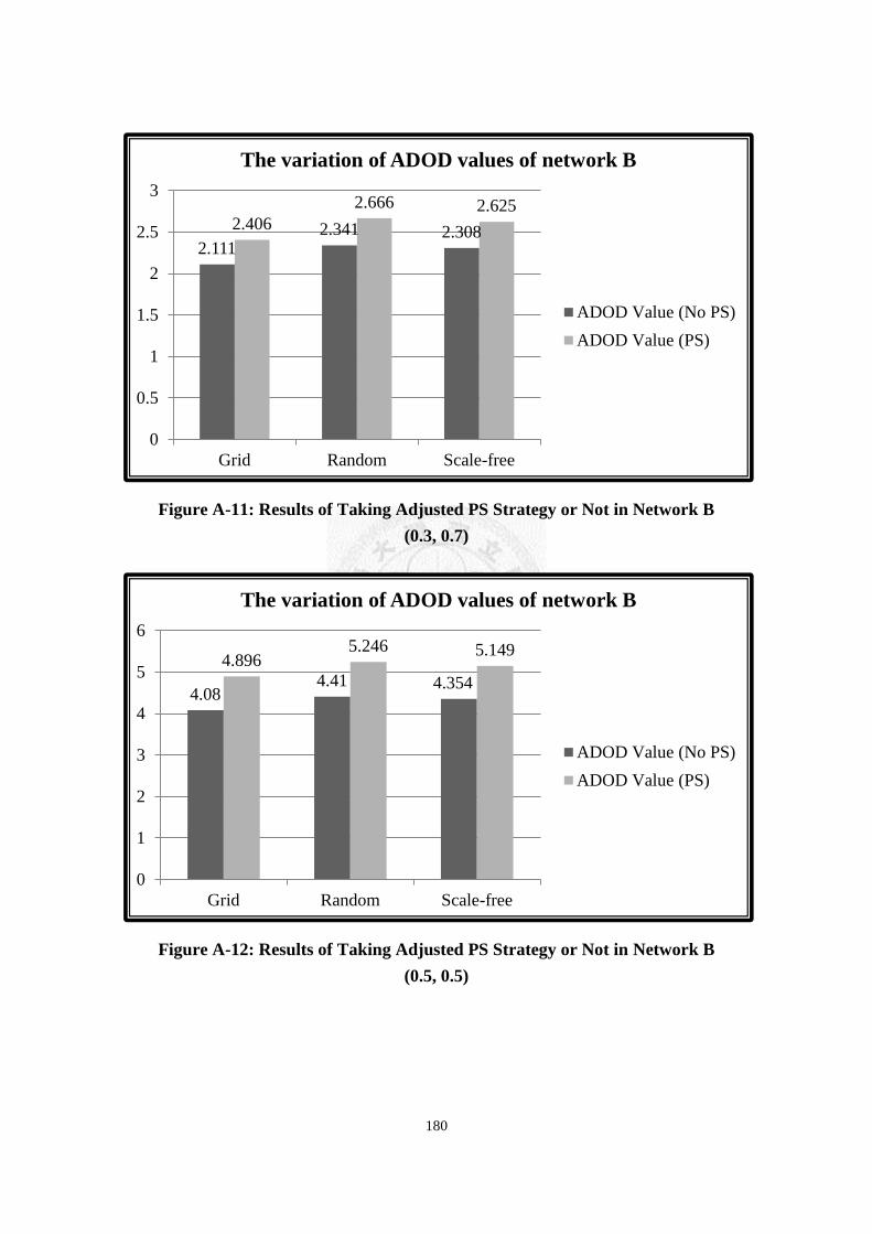
180

Figure A-11: Results of Taking Adjusted PS Strategy or Not in Network B

(0.3, 0.7)


(0.5, 0.5)

2.111 2.341 2.308

2.406

2.666 2.625

0

0.5

1

1.5

2

2.5

3



ADOD Value (No PS)

ADOD Value (PS)

4.08 4.41 4.354

4.896 5.246 5.149

0

1

2

3

4

5

6



ADOD Value (No PS)

ADOD Value (PS)

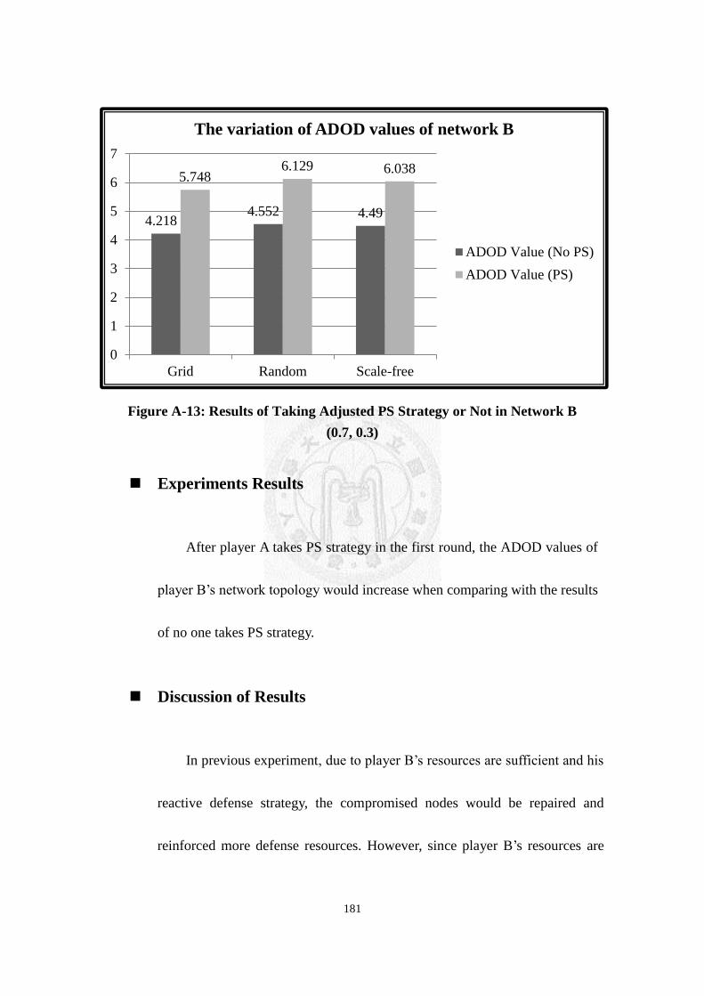
181


(0.7, 0.3)

Experiments Results

After player A takes PS strategy in the first round, the ADOD values of

player B’s network topology would increase when comparing with the results

of no one takes PS strategy.


In previous experiment, due to player B’s resources are sufficient and his

reactive defense strategy, the compromised nodes would be repaired and

reinforced more defense resources. However, since player B’s resources are

4.218 4.552 4.49

5.748 6.129 6.038

0

1

2

3

4

5

6

7



ADOD Value (No PS)

ADOD Value (PS)

182

only half of the original resources (160) in this experiment, the reactive

defense budget is comparatively limited. Furthermore, player A’s attack power

is reinforced when taking adjusted PS strategy in the first round. As a result,

the survivability of network B would decrease in the end.

IV. Comparison of the Variation of ADOD Values between Network A

and Network B

The following three charts of experiment results illustrate the variation of

percentages of ADOD values of network A or network B after taking adjusted PS

strategy. The number in any one of the three charts is obtained by dividing the

ADOD value after taking adjusted PS strategy by the ADOD value of not taking

PS strategy.


Figure A-16.

183

Figure A-14: Adjusted PS Strategy (GD)

Figure A-15: Adjusted PS Strategy (RD)

0.482 0.448 0.422

1.14 1.2

1.363

0

0.2

0.4

0.6

0.8

1

1.2

1.4

1.6

(0.3, 0.7) (0.5, 0.5) (0.7, 0.3)

The variation of percentages of ADOD values

Network A

Network B

0.515 0.461 0.452

1.139 1.19

1.346

0

0.2

0.4

0.6

0.8

1

1.2

1.4

1.6

(0.3, 0.7) (0.5, 0.5) (0.7, 0.3)


Network A

Network B

184

Figure A-16: Adjusted PS Strategy (SF)

Experiments Results

No matter under what kind of network topologies and proportions of

attack to defense resource, the variation of percentages of ADOD values of

Network A in decrease would larger than the variation of percentages of

ADOD values of Network B in increase after player A takes adjusted PS

strategy in the first round.


We take Figure A-14 for example here. Under the proportion of (0.3,

0.7), 1.14 indicates that after taking adjusted PS strategy, the attained ADOD

0.465 0.465 0.466

1.137 1.183

1.345

0

0.2

0.4

0.6

0.8

1

1.2

1.4

1.6

(0.3, 0.7) (0.5, 0.5) (0.7, 0.3)


Network A

Network B

185

value of network B would be 1.14 times of the original ADOD value; on the

other hand, 0.482 indicates that the obtained ADOD value of network A

would become 0.482 times of the original ADOD value. This implies that

taking adjusted PS strategy would make the counterpart’s ADOD increase

while make his own ADOD decrease. Furthermore, the most important

observation from the comparison is that the effect to increase one’s own

network survivability is larger than to decrease the counterpart’s network

survivability after taking adjusted strategy.

Experiment 2: Insufficient Resource Allocation

In previous experiment in section 4.3.2, we obtained a conclusion that the

resource- disadvantaged player should allocate more on attack rather than defense under

the objective of minimizing his own ADOD value and maximizing the counterpart’s

ADOD value, which could be viewed as a strategy of “The best defense is attack.” In

this experiment, we would like to discuss what the experiment results would become

under the circumstance that the amounts of total resources of both players are no longer

as much as (160, 120). Therefore, both players’ total resource would be limited to much

fewer resources as (80, 50), the former one is for player A, and the later one is for player

B. Furthermore, the proportion of attack resource to defense resource that we discussed

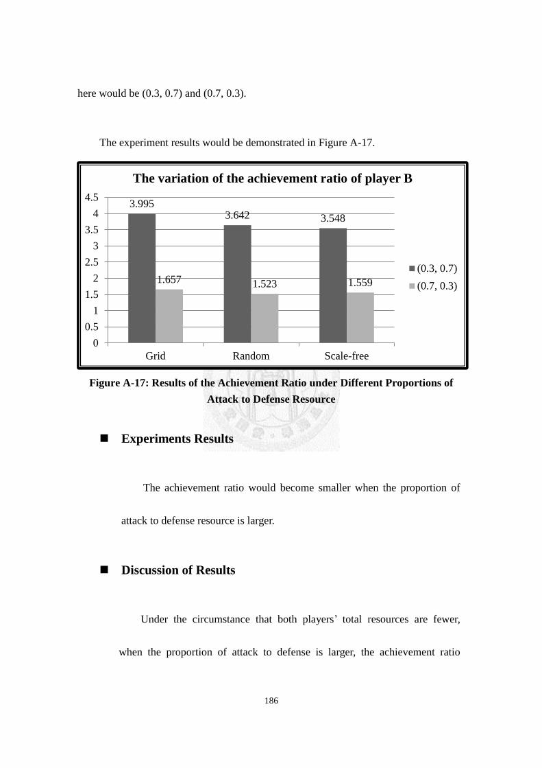
186

here would be (0.3, 0.7) and (0.7, 0.3).

The experiment results would be demonstrated in Figure A-17.

Figure A-17: Results of the Achievement Ratio under Different Proportions of


Experiments Results

The achievement ratio would become smaller when the proportion of

attack to defense resource is larger.


Under the circumstance that both players’ total resources are fewer,

when the proportion of attack to defense is larger, the achievement ratio

3.995 3.642 3.548

1.657 1.523 1.559

0

0.5

1

1.5

2

2.5

3

3.5

4

4.5


The variation of the achievement ratio of player B

(0.3, 0.7)

(0.7, 0.3)

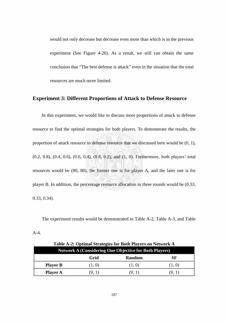
187

would not only decrease but decrease even more than which is in the previous

experiment (See Figure 4-26). As a result, we still can obtain the same

conclusion that “The best defense is attack” even in the situation that the total

resources are much more limited.

Experiment 3: Different Proportions of Attack to Defense Resource

In this experiment, we would like to discuss more proportions of attack to defense

resource to find the optimal strategies for both players. To demonstrate the results, the

proportion of attack resource to defense resource that we discussed here would be (0, 1),

(0.2, 0.8), (0.4, 0.6), (0.6, 0.4), (0.8, 0.2), and (1, 0). Furthermore, both players’ total

resources would be (80, 80), the former one is for player A, and the later one is for

player B. In addition, the percentage resource allocation in three rounds would be (0.33,

0.33, 0.34).

The experiment results would be demonstrated in Table A-2, Table A-3, and Table

A-4.

Table A-2: Optimal Strategies for Both Players on Network A

Network A (Considering One Objective for Both Players)

Grid Random SF

Player B (1, 0) (1, 0) (1, 0)

Player A (0, 1) (0, 1) (0, 1)

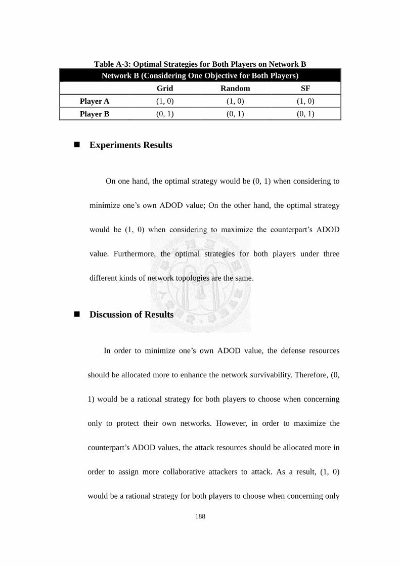
188

Table A-3: Optimal Strategies for Both Players on Network B

Network B (Considering One Objective for Both Players)

Grid Random SF

Player A (1, 0) (1, 0) (1, 0)

Player B (0, 1) (0, 1) (0, 1)

Experiments Results

On one hand, the optimal strategy would be (0, 1) when considering to

minimize one’s own ADOD value; On the other hand, the optimal strategy

would be (1, 0) when considering to maximize the counterpart’s ADOD

value. Furthermore, the optimal strategies for both players under three

different kinds of network topologies are the same.


In order to minimize one’s own ADOD value, the defense resources

should be allocated more to enhance the network survivability. Therefore, (0,

1) would be a rational strategy for both players to choose when concerning

only to protect their own networks. However, in order to maximize the

counterpart’s ADOD values, the attack resources should be allocated more in

order to assign more collaborative attackers to attack. As a result, (1, 0)

would be a rational strategy for both players to choose when concerning only

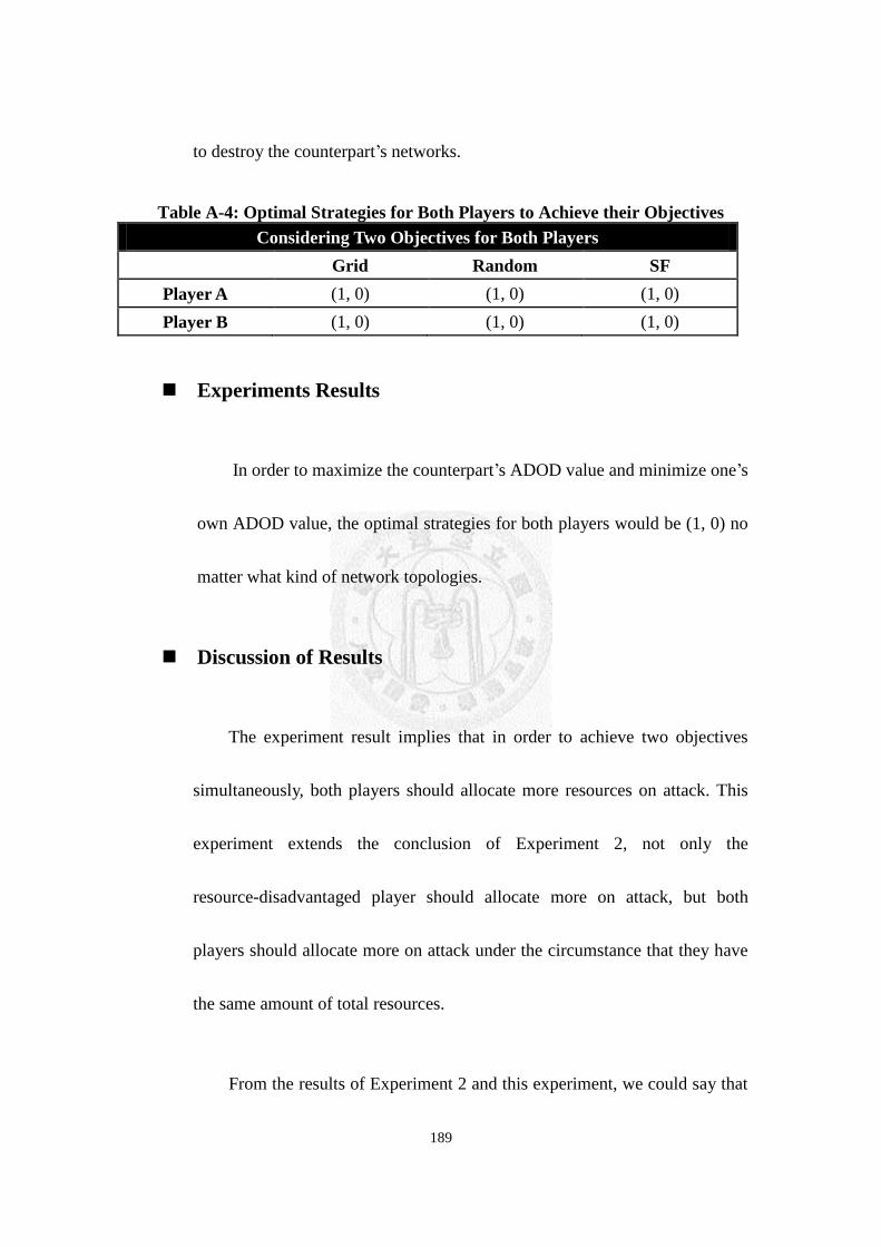
189

to destroy the counterpart’s networks.

Table A-4: Optimal Strategies for Both Players to Achieve their Objectives

Considering Two Objectives for Both Players

Grid Random SF

Player A (1, 0) (1, 0) (1, 0)

Player B (1, 0) (1, 0) (1, 0)

Experiments Results

In order to maximize the counterpart’s ADOD value and minimize one’s

own ADOD value, the optimal strategies for both players would be (1, 0) no

matter what kind of network topologies.


The experiment result implies that in order to achieve two objectives

simultaneously, both players should allocate more resources on attack. This

experiment extends the conclusion of Experiment 2, not only the

resource-disadvantaged player should allocate more on attack, but both

players should allocate more on attack under the circumstance that they have

the same amount of total resources.

From the results of Experiment 2 and this experiment, we could say that

190

the optimal strategy is always attack-first no matter under how much the total

resources are. The policy of “The best defense is attack” stands still.

National Taiwan University Master Thesisoplab.im.ntu.edu.tw/download/Thesis/99/R99725015.pdf ·...

Documents

Transcript of National Taiwan University Master Thesisoplab.im.ntu.edu.tw/download/Thesis/99/R99725015.pdf ·...