MUSIC TRANSFORMER GENERATING MUSIC WITH LONG TERM …

Published as a conference paper at ICLR 2019

MUSIC TRANSFORMER:GENERATING MUSIC WITH LONG-TERM STRUCTURE

Cheng-Zhi Anna Huang∗ Ashish Vaswani Jakob Uszkoreit Noam ShazeerIan Simon Curtis Hawthorne Andrew M. Dai Matthew D. HoffmanMonica Dinculescu Douglas EckGoogle Brain{annahuang,avaswani,usz,noam,iansimon,fjord,adai,mhoffman,noms,deck}@google.com

ABSTRACT

Music relies heavily on repetition to build structure and meaning. Self-referenceoccurs on multiple timescales, from motifs to phrases to reusing of entire sectionsof music, such as in pieces with ABA structure. The Transformer (Vaswaniet al., 2017), a sequence model based on self-attention, has achieved compellingresults in many generation tasks that require maintaining long-range coherence.This suggests that self-attention might also be well-suited to modeling music.In musical composition and performance, however, relative timing is criticallyimportant. Existing approaches for representing relative positional informationin the Transformer modulate attention based on pairwise distance (Shaw et al.,2018). This is impractical for long sequences such as musical compositions becausetheir memory complexity for intermediate relative information is quadratic in thesequence length. We propose an algorithm that reduces their intermediate memoryrequirement to linear in the sequence length. This enables us to demonstratethat a Transformer with our modified relative attention mechanism can generateminute-long compositions (thousands of steps) with compelling structure, generatecontinuations that coherently elaborate on a given motif, and in a seq2seq setupgenerate accompaniments conditioned on melodies1. We evaluate the Transformerwith our relative attention mechanism on two datasets, JSB Chorales and Maestro,and obtain state-of-the-art results on the latter.

1 INTRODUCTION

A musical piece often consists of recurring elements at various levels, from motifs to phrases tosections such as verse-chorus. To generate a coherent piece, a model needs to reference elementsthat came before, sometimes in the distant past, and then repeat, vary, and further develop them tocreate contrast and surprise. Intuitively, self-attention (Parikh et al., 2016) could be a good matchfor this task. Self-attention over its own previous outputs allows an autoregressive model to accessany part of the previously generated output at every step of generation. By contrast, recurrent neuralnetworks have to learn to proactively store elements to be referenced in a fixed size state or memory,making training potentially much more difficult. We believe that repeating self-attention in multiple,successive layers of a Transformer decoder (Vaswani et al., 2017) can help capture the multiple levelsat which self-referential phenomena exist in music.

In its original formulation, the Transformer relies on absolute position representations, using eitherpositional sinusoids or learned position embeddings that are added to the per-position input repre-sentations. Recurrent and convolutional neural networks instead model position in relative terms:RNNs through their recurrence over the positions in their input, and CNNs by applying kernels thateffectively choose which parameters to apply based on the relative position of the covered inputrepresentations.

∗Google AI Resident. Correspondence to: Cheng-Zhi Anna Huang <[email protected]>1Samples are available for listening at

https://goo.gl/magenta/music-transformer-examples.Later blog post at https://magenta.tensorflow.org/music-transformer

1

https://goo.gl/magenta/music-transformer-examples

https://magenta.tensorflow.org/music-transformer


Music has multiple dimensions along which relative differences arguably matter more than theirabsolute values; the two most prominent are timing and pitch. To capture such pairwise relationsbetween representations, Shaw et al. (2018) introduce a relation-aware version of self-attention whichthey use successfully to modulate self-attention by the distance between two positions. We extendthis approach to capture relative timing and optionally also pitch, which yields improvement in bothsample quality and perplexity for the JSB Chorales dataset. As opposed to the original Transformer,samples from a Transformer with our relative attention mechanism maintain the regular timing gridpresent in this dataset. The model furthermore captures global timing, giving rise to regular phrases.

The original formulation of relative attention (Shaw et al., 2018) requires O(L2D) memory where Lis the sequence length and D is the dimension of the model’s hidden state. This is prohibitive for longsequences such as those found in the Maestro dataset of human-performed virtuosic, classical pianomusic (Hawthorne et al., 2019). In Section 3.4, we show how to reduce the memory requirements toO(LD), making it practical to apply relative attention to long sequences.

The Maestro dataset consists of MIDI recorded from performances of competition participants,bearing expressive dynamics and timing on a less than 10-millisecond granularity. Discretizing timein a fixed grid on such a resolution would yield unnecessarily long sequences as not all events changeon the same timescale. We hence adopt a sparse, MIDI-like, event-based representation from (Ooreet al., 2018), allowing a minute of music with a 10-millisecond resolution to be represented atlengths around 2K. This is in contrast to a 6K to 18K length that would be needed on a serializedmulti-attribute fixed-grid representation. As position in sequence no longer corresponds to time, apriori it is not obvious that relative attention should work as well with such a representation. However,we will show in Section 4.2 that it does improve perplexity and sample quality over strong baselines.

We speculate that idiomatic piano gestures such as scales, arpeggios and other motifs all exhibit acertain grammar and recur periodically, hence knowing their relative positional distances makes iteasier to model this regularity. This inductive bias towards learning relational information, as opposedto patterns based on absolute position, suggests that the Transformer with relative attention couldgeneralize beyond the lengths it was trained on, which our experiments in Section 4.2.1 confirm.

1.1 CONTRIBUTIONS

Domain contributions We show the first successful use of Transformers in generating musicthat exhibits long-term structure. Before our work, LSTMs were used at timescales of 15s (~500tokens) of piano performances (Oore et al., 2018). Our work demonstrates that Transformers notonly achieve state-of-the-art perplexity on modeling these complex expressive piano performances,but can also generate them at the scale of minutes (thousands of tokens) with remarkable internalconsistency. Our relative self-attention formulation is essential to the model’s quality. In listeningtests (see Section 4.2.3), samples from models with relative self-attention were perceived as morecoherent than the baseline Transformer model (Vaswani et al., 2017). Relative attention not onlyenables Transformers to generate continuations that elaborate on a given motif, but also to generalizeand generate in consistent fashion beyond the length it was trained on (see Section 4.2.1). In aseq2seq setup, Transformers can generate accompaniments conditioned on melodies, enabling usersto interact with the model.

Algorithmic contributions The space complexity of the relative self-attention mechanism in itsoriginal formulation (Shaw et al., 2018) made it infeasible to train on sequences of sufficient lengthto capture long-range structure in longer musical compositions. To address this, we present a crucialalgorithmic improvement to the relative self-attention mechanism, dramatically reducing its memoryrequirements from O(L2D) to O(LD). For example, the memory consumption per layer is reducedfrom 8.5 GB to 4.2 MB (per head from 1.1 GB to 0.52 MB) for a sequence of length L = 2048 andhidden-state size D = 512 (per head Dh = D

H = 64, where number of heads is H = 8) (see Table 1),allowing us to use GPUs to train the relative self-attention Transformer on long sequences.

2 RELATED WORK

Sequence models have been the canonical choice for modeling music, from Hidden Markov Modelsto RNNs and Long Short Term Memory networks (e.g., Eck & Schmidhuber, 2002; Liang, 2016;Oore et al., 2018), to bidirectional LSTMs (e.g., Hadjeres et al., 2017). Successful application of

2


sequential models to polyphonic music often requires serializing the musical score or performanceinto a single sequence, for example by interleaving different instruments or voices. Alternatively,a 2D pianoroll-like representation (see A.1 for more details) can be decomposed into a sequenceof multi-hot pitch vectors, and their joint probability distributions can be captured using RestrictedBoltzmann Machines (Smolensky, 1986; Hinton et al., 2006) or Neural Autoregressive DistributionEstimators (NADE; Larochelle & Murray, 2011). Pianorolls are also image-like and can be modeledby CNNs trained either as generative adversarial networks (GAN; Goodfellow et al., 2014). (e.g.,Dong et al., 2018) or as orderless NADEs (Uria et al., 2014; 2016) (e.g., Huang et al., 2017).

Lattner et al. (2018) use self-similarity in style-transfer fashion, where the self-similarity structure ofa piece serves as a template objective for gradient descent to impose similar repetition structure on aninput score. Self-attention can be seen as a generalization of self-similarity; the former maps the inputthrough different projections to queries and keys, and the latter uses the same projection for both.

Dot-product self-attention is the mechanism at the core of the Transformer, and several recent workshave focused on applying and improving it for image generation, speech, and summarization (Parmaret al., 2018; Povey et al., 2018; Liu et al., 2018). A key challenge encountered by each of these effortsis scaling attention computationally to long sequences. This is because the time and space complexityof self-attention grows quadratically in the sequence length. For relative self-attention (Shaw et al.,2018) this is particularly problematic as the space complexity also grows linearly in the dimension,or depth, of the per-position representations.

3 MODEL

3.1 DATA REPRESENTATION

We take a language-modeling approach to training generative models for symbolic music. Hencewe represent music as a sequence of discrete tokens, with the vocabulary determined by the dataset.Datasets in different genres call for different ways of serializing polyphonic music into a singlestream and also discretizing time.

The JSB Chorale dataset consists of four-part scored choral music, which can be represented as amatrix where rows correspond to voices and columns to time discretized to sixteenth notes. Thematrix’s entries are integers that denote which pitch is being played. This matrix can than be serializedin raster-scan fashion by first going down the rows and then moving right through the columns (see A.1for more details). Compared to JSB Chorale, the piano performance data in the Maestro datasetincludes expressive timing information at much finer granularity and more voices. For the Maestrodataset we therefore use the performance encoding proposed by Oore et al. (2018) which consists of avocabulary of 128 NOTE_ON events, 128 NOTE_OFFs, 100 TIME_SHIFTs allowing for expressivetiming at 10ms and 32 VELOCITY bins for expressive dynamics (see A.2 for more details).

3.2 BACKGROUND: SELF-ATTENTION IN TRANSFORMER

The Transformer decoder is a autoregressive generative model that uses primarily self-attentionmechanisms, and learned or sinusoidal position information. Each layer consists of a self-attentionsub-layer followed by a feedforward sub-layer.

The attention layer first transforms a sequence of L D-dimensional vectors X = (x1, x2, . . . , xL)into queries Q = XWQ, keys K = XWK , and values V = XWV , where WQ, WK , and WV areeach D ×D square matrices. Each L×D query, key, and value matrix is then split into H L×Dh

parts or attention heads, indexed by h, and with dimension Dh = DH , which allow the model to focus

on different parts of the history. The scaled dot-product attention computes a sequence of vectoroutputs for each head as

Zh = Attention(Qh,Kh, V h) = Softmax(QhKh>√Dh

)V h. (1)

The attention outputs for each head are concatenated and linearly transformed to get Z, a L by Ddimensional matrix. A upper triangular mask ensures that queries cannot attend to keys later in thesequence. For other details of the Transfomer model, such as residual connections and learning rates,the reader can refer Vaswani et al. (2017). The feedforward (FF) sub-layer then takes the output Z

3


from the previous attention sub-layer, and performs two layers of point-wise dense layers on the depthD dimension, as shown in Equation 2. W1,W2, b1, b2 are weights and biases of those two layers.

FF(Z) = ReLU(ZW1 + b1)W2 + b2 (2)

3.3 RELATIVE POSITIONAL SELF-ATTENTION

As the Transformer model relies solely on positional sinusoids to represent timing information, Shawet al. (2018) introduced relative position representations to allow attention to be informed by how fartwo positions are apart in a sequence. This involves learning a separate relative position embeddingEr of shape (H,L,Dh), which has an embedding for each possible pairwise distance r = jk − iqbetween a query and key in position iq and jk respectively. The embeddings are ordered from distance−L+ 1 to 0, and are learned separately for each head. In Shaw et al. (2018), the relative embeddingsinteract with queries and give rise to a Srel, an L× L dimensional logits matrix which modulates theattention probabilities for each head as:

RelativeAttention = Softmax(QK> + Srel

√Dh

)V. (3)

We dropped head indices for clarity. Our work uses the same approach to infuse relative distanceinformation in the attention computation, while significantly improving upon the memory footprintfor computing Srel. For each head, Shaw et al. (2018) instantiate an intermediate tensor R of shape(L,L,Dh), containing the embeddings that correspond to the relative distances between all keys andqueries. Q is then reshaped to an (L, 1, Dh) tensor, and Srel = QR>.2 This incurs a total spacecomplexity of O(L2D), restricting its application to long sequences.

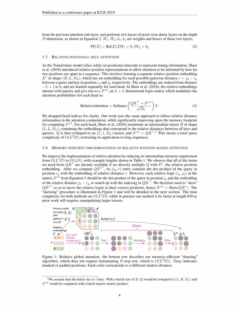
3.4 MEMORY EFFICIENT IMPLEMENTATION OF RELATIVE POSITION-BASED ATTENTION

We improve the implementation of relative attention by reducing its intermediate memory requirementfrom O(L2D) to O(LD), with example lengths shown in Table 1. We observe that all of the termswe need from QR> are already available if we directly multiply Q with Er, the relative positionembedding. After we compute QEr>, its (iq, r) entry contains the dot product of the query inposition iq with the embedding of relative distance r. However, each relative logit (iq, jk) in thematrix Srel from Equation 3 should be the dot product of the query in position iq and the embeddingof the relative distance jk − iq , to match up with the indexing in QK>. We therefore need to “skew”QEr> so as to move the relative logits to their correct positions, hence Srel = Skew(QEr). The“skewing” procedure is illustrated in Figure 1 and will be detailed in the next section. The timecomplexity for both methods are O(L2D), while in practice our method is 6x faster at length 650 asprior work still requires manipulating larger tensors.

Figure 1: Relative global attention: the bottom row describes our memory-efficient “skewing”algorithm, which does not require instantiating R (top row, which is O(L2D)). Gray indicatesmasked or padded positions. Each color corresponds to a different relative distance.

2We assume that the batch size is 1 here. With a batch size of B, Q would be reshaped to (L,B,Dh) andSrel would be computed with a batch matrix–matrix product.

4


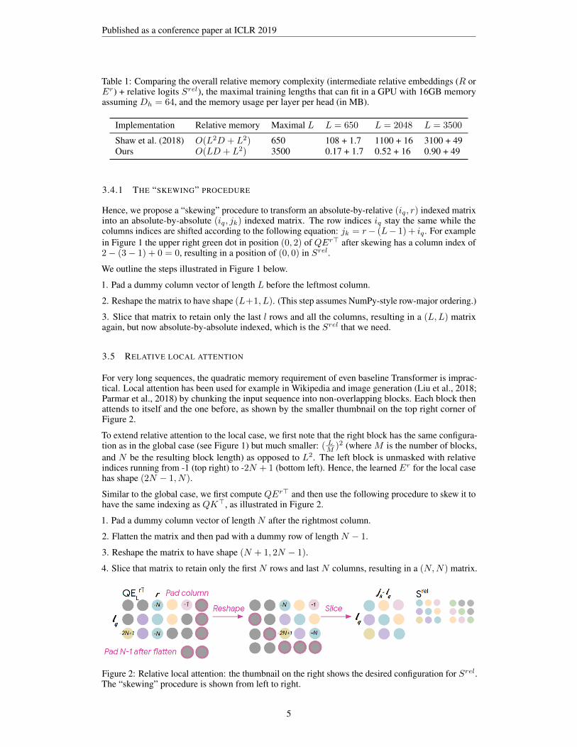
Table 1: Comparing the overall relative memory complexity (intermediate relative embeddings (R orEr) + relative logits Srel), the maximal training lengths that can fit in a GPU with 16GB memoryassuming Dh = 64, and the memory usage per layer per head (in MB).

Implementation Relative memory Maximal L L = 650 L = 2048 L = 3500

Shaw et al. (2018) O(L2D + L2) 650 108 + 1.7 1100 + 16 3100 + 49Ours O(LD + L2) 3500 0.17 + 1.7 0.52 + 16 0.90 + 49

3.4.1 THE “SKEWING” PROCEDURE

Hence, we propose a “skewing” procedure to transform an absolute-by-relative (iq, r) indexed matrixinto an absolute-by-absolute (iq, jk) indexed matrix. The row indices iq stay the same while thecolumns indices are shifted according to the following equation: jk = r− (L− 1)+ iq . For examplein Figure 1 the upper right green dot in position (0, 2) of QEr> after skewing has a column index of2− (3− 1) + 0 = 0, resulting in a position of (0, 0) in Srel.

We outline the steps illustrated in Figure 1 below.

1. Pad a dummy column vector of length L before the leftmost column.

2. Reshape the matrix to have shape (L+1, L). (This step assumes NumPy-style row-major ordering.)

3. Slice that matrix to retain only the last l rows and all the columns, resulting in a (L,L) matrixagain, but now absolute-by-absolute indexed, which is the Srel that we need.

3.5 RELATIVE LOCAL ATTENTION

For very long sequences, the quadratic memory requirement of even baseline Transformer is imprac-tical. Local attention has been used for example in Wikipedia and image generation (Liu et al., 2018;Parmar et al., 2018) by chunking the input sequence into non-overlapping blocks. Each block thenattends to itself and the one before, as shown by the smaller thumbnail on the top right corner ofFigure 2.

To extend relative attention to the local case, we first note that the right block has the same configura-tion as in the global case (see Figure 1) but much smaller: ( L

M )2 (where M is the number of blocks,and N be the resulting block length) as opposed to L2. The left block is unmasked with relativeindices running from -1 (top right) to -2N + 1 (bottom left). Hence, the learned Er for the local casehas shape (2N − 1, N).

Similar to the global case, we first compute QEr> and then use the following procedure to skew it tohave the same indexing as QK>, as illustrated in Figure 2.

1. Pad a dummy column vector of length N after the rightmost column.

2. Flatten the matrix and then pad with a dummy row of length N − 1.

3. Reshape the matrix to have shape (N + 1, 2N − 1).

4. Slice that matrix to retain only the first N rows and last N columns, resulting in a (N,N) matrix.

Figure 2: Relative local attention: the thumbnail on the right shows the desired configuration for Srel.The “skewing” procedure is shown from left to right.

5


4 EXPERIMENTS

4.1 J.S. BACH CHORALES

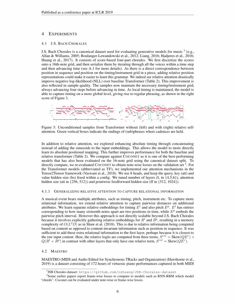
J.S. Bach Chorales is a canonical dataset used for evaluating generative models for music 3 (e.g.,Allan & Williams, 2005; Boulanger-Lewandowski et al., 2012; Liang, 2016; Hadjeres et al., 2016;Huang et al., 2017). It consists of score-based four-part chorales. We first discretize the scoresonto a 16th-note grid, and then serialize them by iterating through all the voices within a time stepand then advancing time (see A.1 for more details). As there is a direct correspondence betweenposition in sequence and position on the timing/instrument grid in a piece, adding relative positionrepresentations could make it easier to learn this grammar. We indeed see relative attention drasticallyimprove negative log-likelihood (NLL) over baseline Transformer (Table 2). This improvement isalso reflected in sample quality. The samples now maintain the necessary timing/instrument grid,always advancing four steps before advancing in time. As local timing is maintained, the model isable to capture timing on a more global level, giving rise to regular phrasing, as shown in the rightscore of Figure 3.

Figure 3: Unconditioned samples from Transformer without (left) and with (right) relative self-attention. Green vertical boxes indicate the endings of (sub)phrases where cadences are held.

In addition to relative attention, we explored enhancing absolute timing through concatenatinginstead of adding the sinusoids to the input embeddings. This allows the model to more directlylearn its absolute positional mapping. This further improves performance for both the baseline andrelative transformer (Table 2). We compare against COCONET as it is one of the best-performingmodels that has also been evaluated on the 16-note grid using the canonical dataset split. Todirectly compare, we re-evaluated COCONET to obtain note-wise losses on the validation set 4. Forthe Transformer models (abbreviated as TF), we implemented our attention mechanisms in theTensor2Tensor framework (Vaswani et al., 2018). We use 8 heads, and keep the query, key (att) andvalue hidden size (hs) fixed within a config. We tuned number of layers (L in {4,5,6}), attentionhidden size (att in {256, 512}) and pointwise feedforward hidden size (ff in {512, 1024}).

4.1.1 GENERALIZING RELATIVE ATTENTION TO CAPTURE RELATIONAL INFORMATION

A musical event bears multiple attributes, such as timing, pitch, instrument etc. To capture morerelational information, we extend relative attention to capture pairwise distances on additionalattributes. We learn separate relative embeddings for timing Et and also pitch Ep. Et has entriescorresponding to how many sixteenth notes apart are two positions in time, while Ep embeds thepairwise pitch interval. However this approach is not directly scalable beyond J.S. Bach Choralesbecause it involves explicitly gathering relative embeddings for Rt and Rp, resulting in a memorycomplexity of O(L2D) as in Shaw et al. (2018). This is due to relative information being computedbased on content as opposed to content-invariant information such as position in sequence. It wassufficient to add these extra relational information to the first layer, perhaps because it is closest tothe raw input content. Here, the relative logits are computed from three terms, Srel = Skew(QEr) +Q(Rt +Rp) in contrast with other layers that only have one relative term, Srel = Skew(QEr).

4.2 MAESTRO

MAESTRO (MIDI and Audio Edited for Synchronous TRacks and Organization) (Hawthorne et al.,2019) is a dataset consisting of 172 hours of virtuosic piano performances captured in both MIDI

3JSB Chorales dataset: https://github.com/czhuang/JSB-Chorales-dataset4Some earlier papers report frame-wise losses to compare to models such as RNN-RBM which model

“chords”. Coconet can be evaluated under note-wise or frame-wise losses.

6

https://github.com/czhuang/JSB-Chorales-dataset


and audio format 5. It is curated from the Piano-e-Competitions 6, and proposes a train / valid / testsplit where the same composition, even if performed by multiple contestants, only appears in onesplit. The result is 295 / 60 / 75 unique compositions, corresponding to 954 / 105 / 125 performancesthat last for 140 / 15 / 17 hours and contain 5.06 / 0.54 / 0.57 million notes. The polyphonic MIDIperformances contain both expressive dynamics and timing and we serialize them into sequencesof event-based tokens as introduced in Oore et al. (2018) (see Section A.2 for more details on theencoding procedure).

We train on random crops of 2048-token sequences and employ two kinds of data augmentation: pitchtranspositions uniformly sampled from {−3,−2, . . . , 2, 3} half-steps, and time stretches uniformlysampled from the set {0.95, 0.975, 1.0, 1.025, 1.05}. For evaluation, we segment each sequencesequentially into 2048 length subsequences and also keep the last subsequences that are of shorterlengths. This results in 1128 and 1183 subsequences in the validation and test set respectively. Eachsubsequence is then evaluated by running the model forward once with teaching forcing. As thesubsequences vary in length, the overall negative loglikelihood (NLL) is averaged entirely on thetoken level.

Table 2: Note-wise validation NLL (nats/token) on J.S. Bach Chorales where each token is a 16thnote. NLL is improved by using the Transformer with our memory-efficient relative global attentionformulation, also when including additional positional and relational information.

Model variation Validation

COCONET (CNN, chronological, 64L, 128 3x3f) 0.436COCONET (CNN, orderless, 64L, 128 3x3f) 0.238 7

Transformer (TF) baseline (5L, 256hs, 256att, 1024ff, 8h) 0.417+ concat positional sinusoids 0.398+ concat positional sinusoids, include instrument labels 0.370

TF with efficient relative attention (ours) (5L, 512hs, 512att, 512ff, 256r, 8h) 0.357+ concat positional sinusoids, include instrument labels 0.347

+ relative pitch and time 0.335

Table 3: Validation NLL (nats/token) for Maestro dataset, with event-based representation withlengths L = 2048. Training and/or evaluating on different lengths will result in different lossesbecause the amount of context available to the model would be different. The Transformer with ourmemory-efficient relative attention formulation achieves state-of-the-art results.

Model variation Validation Test

PERFORMANCE RNN (LSTM) (3L, 1024hs) 2.094 —LSTM with attention (3L, 1024hs, 1024att) 2.066 —

Transformer (TF) baseline (8L, 384hs, 512att, 1024fs, 0.2d) 1.835 1.813local attention (10L, 512bs, 0.3d) 1.895 1.888efficient relative local attention (ours) (8L, 512bs, 0.2d) 1.873 1.861efficient relative global attention (ours) (8L, 1024r, 0.2d) 1.808 1.791

We compare our results to PerformanceRNN (LSTM, which first used this dataset) (Oore et al.,2018) and LookBack RNN (LSTM with attention) (Waite, 2016). LookBack RNN uses an inputrepresentation that requires monophonic music with barlines which is information that is not present

5Maestro dataset: urlhttps://magenta.tensorflow.org/datasets/maestro6Piano-e-Competition: http://www.piano-e-competition.com/7COCONET is an instance of OrderlessNADE, which approximates a mixture model over orderings where

orderings are assumed to be uniformly distributed. Hence, its loss is computed by averaging losses over multiplerandom orderings. The current row in the table reports this loss. In contrast, the row above corresponds toevaluating Coconet as an autoregressive model under the chronological ordering. Huang et al. (2017) showthat sample quality is better when using Gibbs sampling (which uses conditionals from multiple orderings) asopposed to autoregressive generation (which only uses conditionals from one ordering).

7

http://www.piano-e-competition.com/


in performed polyphonic music data, hence we simply adopt their architecture. Table 3 shows thatTransformer-based architectures fits this dataset better than LSTM-based models.

We implemented our attention mechanisms in the Tensor2Tensor framework (Vaswani et al., 2018),and used the default hyperparameters for training, with 0.1 learning rate and early stopping. Wecompare four architectures, varying on two axes: global versus local, and regular versus relativeattention. We found that reducing the query and key channel size (att) to three forth of the hiddensize (hs) works well for this dataset and used this setup for all of the models, while tuning on numberof layers (L) and dropout rate (d). We use block size (bs) 512 for local attention (Liu et al., 2018;Parmar et al., 2018). For relative global attention, the maximum relative distance to consider is set tohalf the training sequence length. For relative local attention, it is set to the full memory length whichis two blocks long.

Table 3 shows that our memory-efficient relative attention formulations outperform regular attentionin both the global and the local case. When looking at the other axes, we see global attentionoutperforming local attention in both the relative and regular case. Global attention may have theadvantage of being able to directly look back for repeating motifs. With a larger dataset, localattention may fare well as it allows for much deeper models and longer sequences, as seen in text andimage generation work (Liu et al., 2018; Parmar et al., 2018)). In turn, both domains could benefitfrom the use of relative local attention.

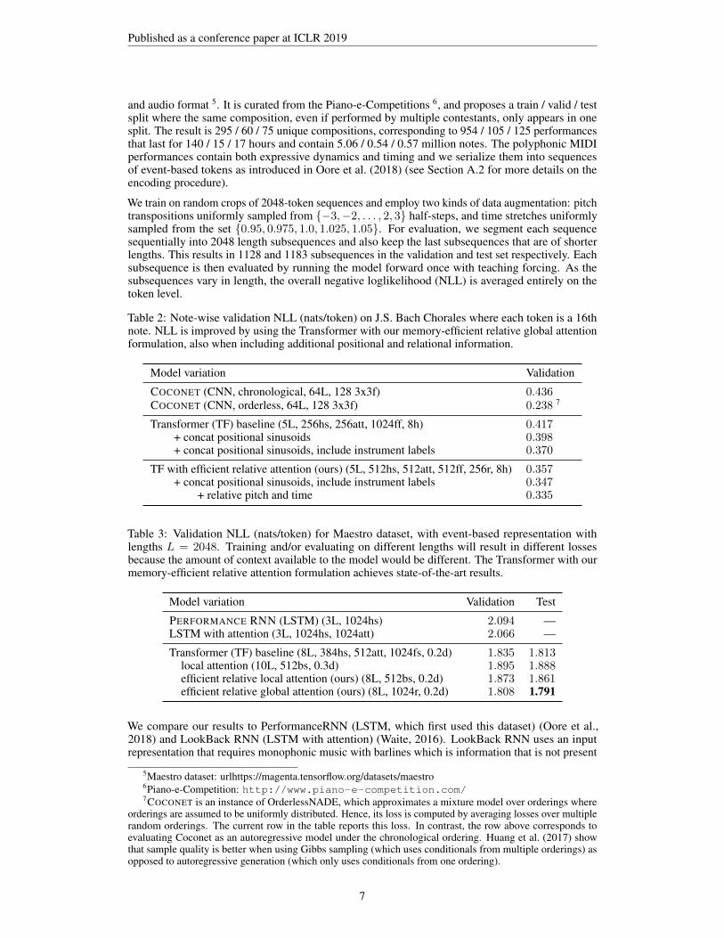
Figure 4: Transformer with relative attention (three random samples on the top row) when given aninitial motif (top left) generates continuations with more repeated motifs and structure then baselineTransformer (middle row) and PerformanceRNN (bottom row).

4.2.1 QUALITATIVE PRIMING EXPERIMENTS

When primed with an initial motif (Chopin’s Étude Op. 10, No. 5) shown in the top left corner ofFigure 4, we see the models perform qualitatively differently. Transformer with relative attentionelaborates the motif and creates phrases with clear contour which are repeated and varied. BaselineTransformer uses the motif in a more uniform fashion, while LSTM uses the motif initially butsoon drifts off to other material. Note that the generated samples are twice as long as the trainingsequences. Relative attention was able to generalize to lengths longer than trained but baselineTransformer deteriorates beyond its training length. See Appendix C for visualizations of how ourRelative Transformer attends to past motifs.

4.2.2 HARMONIZATION: CONDITIONING ON MELODY

To explore the sequence-to-sequence setup of Transformers, we experimented with a conditionedgeneration task where the encoder takes in a given melody and the decoder has to realize the entireperformance, i.e. melody plus accompaniment. The melody is encoded as a sequence of tokens as inWaite (2016), quantized to a 100ms grid, while the decoder uses the performance encoding describedin Section 3.1 (and further illustrated in A.2). We use relative attention on the decoder side and showin Table 4 that it also improves performance.

8


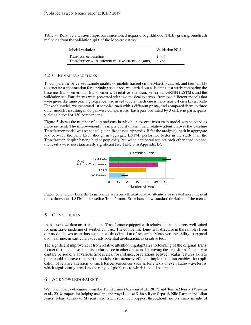
Table 4: Relative attention improves conditioned negative logliklihood (NLL) given groundtruthmelodies from the validation split of the Maestro dataset.

Model variation Validation NLL

Transformer baseline 2.066Transformer with efficient relative attention (ours) 1.786

4.2.3 HUMAN EVALUATIONS

To compare the perceived sample quality of models trained on the Maestro dataset, and their abilityto generate a continuation for a priming sequence, we carried out a listening test study comparing thebaseline Transformer, our Transformer with relative-attention, PerformanceRNN (LSTM), and thevalidation set. Participants were presented with two musical excerpts (from two different models thatwere given the same priming sequence) and asked to rate which one is more musical on a Likert scale.For each model, we generated 10 samples each with a different prime, and compared them to threeother models, resulting in 60 pairwise comparisons. Each pair was rated by 3 different participants,yielding a total of 180 comparisons.

Figure 5 shows the number of comparisons in which an excerpt from each model was selected asmore musical. The improvement in sample quality from using relative attention over the baselineTransformer model was statistically significant (see Appendix B for the analysis), both in aggregateand between the pair. Even though in aggregate LSTMs performed better in the study than theTransformer, despite having higher perplexity, but when compared against each other head to head,the results were not statistically significant (see Table 5 in Appendix B).

(Ours)

Figure 5: Samples from the Transformer with our efficient relative attention were rated more musicalmore times than LSTM and baseline Transformer. Error bars show standard deviation of the mean.

5 CONCLUSION

In this work we demonstrated that the Transformer equipped with relative attention is very well-suitedfor generative modeling of symbolic music. The compelling long-term structure in the samples fromour model leaves us enthusiastic about this direction of research. Moreover, the ability to expandupon a prime, in particular, suggests potential applications as creative tool.

The significant improvement from relative attention highlights a shortcoming of the original Trans-former that might also limit its performance in other domains. Improving the Transformer’s ability tocapture periodicity at various time scales, for instance, or relations between scalar features akin topitch could improve time-series models. Our memory-efficient implementation enables the appli-cation of relative attention to much longer sequences such as long texts or even audio waveforms,which significantly broadens the range of problems to which it could be applied.

6 ACKNOWLEDGEMENT

We thank many colleagues from the Transformer (Vaswani et al., 2017) and Tensor2Tensor (Vaswaniet al., 2018) papers for helping us along the way: Lukasz Kaiser, Ryan Sepassi, Niki Parmar and LlionJones. Many thanks to Magenta and friends for their support throughout and for many insightful

9


discussions: Jesse Engel, Adam Roberts, Fred Bertsch, Erich Elsen, Sander Dieleman, Sageev Oore,Carey Radebaugh, Natasha Jaques, Daphne Ippolito, Sherol Chan, Vida Vakilotojar, Dustin Tran,Ben Poole and Tim Cooijmans.

REFERENCES

Moray Allan and Christopher KI Williams. Harmonising chorales by probabilistic inference. Advancesin neural information processing systems, 17:25–32, 2005.

Nicolas Boulanger-Lewandowski, Yoshua Bengio, and Pascal Vincent. Modeling temporal dependen-cies in high-dimensional sequences: Application to polyphonic music generation and transcription.International Conference on Machine Learning, 2012.

Hao-Wen Dong, Wen-Yi Hsiao, Li-Chia Yang, and Yi-Hsuan Yang. Musegan: Multi-track sequentialgenerative adversarial networks for symbolic music generation and accompaniment. In Proceedingsof the AAAI Conference on Artificial Intelligence, 2018.

Douglas Eck and Juergen Schmidhuber. Finding temporal structure in music: Blues improvisationwith lstm recurrent networks. In Proceedings of the 12th IEEE Workshop on Neural Networks forSignal Processing, 2002.

Ian Goodfellow, Jean Pouget-Abadie, Mehdi Mirza, Bing Xu, David Warde-Farley, Sherjil Ozair,Aaron Courville, and Yoshua Bengio. Generative adversarial nets. In Advances in neural informa-tion processing systems, pp. 2672–2680, 2014.

Gaëtan Hadjeres, Jason Sakellariou, and François Pachet. Style imitation and chord invention inpolyphonic music with exponential families. arXiv preprint arXiv:1609.05152, 2016.

Gaëtan Hadjeres, François Pachet, and Frank Nielsen. Deepbach: a steerable model for bach choralesgeneration. In International Conference on Machine Learning, pp. 1362–1371, 2017.

Curtis Hawthorne, Andriy Stasyuk, Adam Roberts, Ian Simon, Cheng-Zhi Anna Huang, SanderDieleman, Erich Elsen, Jesse Engel, and Douglas Eck. Enabling factorized piano music modelingand generation with the maestro dataset. In International Conference on Learning Representations,2019.

Geoffrey E Hinton, Simon Osindero, and Yee-Whye Teh. A fast learning algorithm for deep beliefnets. Neural computation, 18(7):1527–1554, 2006.

Cheng-Zhi Anna Huang, Tim Cooijmans, Adam Roberts, Aaron Courville, and Doug Eck. Coun-terpoint by convolution. In Proceedings of the International Conference on Music InformationRetrieval, 2017.

Hugo Larochelle and Iain Murray. The neural autoregressive distribution estimator. In AISTATS,volume 1, pp. 2, 2011.

Stefan Lattner, Maarten Grachten, and Gerhard Widmer. Imposing higher-level structure in poly-phonic music generation using convolutional restricted boltzmann machines and constraints.Journal of Creative Music Systems, 2(2), 2018.

Feynman Liang. Bachbot: Automatic composition in the style of bach chorales. Masters thesis,University of Cambridge, 2016.

Peter J Liu, Mohammad Saleh, Etienne Pot, Ben Goodrich, Ryan Sepassi, Lukasz Kaiser, and NoamShazeer. Generating wikipedia by summarizing long sequences. In Proceedings of the InternationalConference on Learning Representations, 2018.

Sageev Oore, Ian Simon, Sander Dieleman, Douglas Eck, and Karen Simonyan. This time withfeeling: Learning expressive musical performance. arXiv preprint arXiv:1808.03715, 2018.

Ankur Parikh, Oscar Täckström, Dipanjan Das, and Jakob Uszkoreit. A decomposable attentionmodel for natural language inference. In Proceedings of the Conference on Empirical Methods inNatural Language Processing, 2016.

10


Niki Parmar, Ashish Vaswani, Jakob Uszkoreit, Łukasz Kaiser, Noam Shazeer, and Alexander Ku.Image transformer. In Proceedings of the International Conference on Machine Learning, 2018.

Daniel Povey, Hossein Hadian, Pegah Ghahremani, Ke Li, and Sanjeev Khudanpur. A time-restrictedself-attention layer for ASR. In Proceddings of the IEEE International Conference on Acoustics,Speech and Signal Processing (ICASSP). IEEE, 2018.

Peter Shaw, Jakob Uszkoreit, and Ashish Vaswani. Self-attention with relative position representa-tions. In Proceedings of the Conference of the North American Chapter of the Association forComputational Linguistics: Human Language Technologies, volume 2, 2018.

Paul Smolensky. Information processing in dynamical systems: Foundations of harmony theory.Technical report, DTIC Document, 1986.

Benigno Uria, Iain Murray, and Hugo Larochelle. A deep and tractable density estimator. InInternational Conference on Machine Learning, pp. 467–475, 2014.

Benigno Uria, Marc-Alexandre Côté, Karol Gregor, Iain Murray, and Hugo Larochelle. Neuralautoregressive distribution estimation. The Journal of Machine Learning Research, 17(1):7184–7220, 2016.

Ashish Vaswani, Noam Shazeer, Niki Parmar, Jakob Uszkoreit, Llion Jones, Aidan N Gomez, ŁukaszKaiser, and Illia Polosukhin. Attention is all you need. In Advances in Neural InformationProcessing Systems, 2017.

Ashish Vaswani, Samy Bengio, Eugene Brevdo, Francois Chollet, Aidan N. Gomez, Stephan Gouws,Llion Jones, Łukasz Kaiser, Nal Kalchbrenner, Niki Parmar, Ryan Sepassi, Noam Shazeer, andJakob Uszkoreit. Tensor2tensor for neural machine translation. CoRR, abs/1803.07416, 2018.

Elliot Waite. Generating long-term structure in songs and stories. https://magenta.tensorflow.org/2016/07/15/lookback-rnn-attention-rnn, 2016.

11

https://magenta.tensorflow.org/2016/07/15/lookback-rnn-attention-rnn

https://magenta.tensorflow.org/2016/07/15/lookback-rnn-attention-rnn


A DOMAIN-SPECIFIC REPRESENTATIONS

Adapting sequence models for music requires making decisions on how to serialize a polyphonictexture. The data type, whether score or performance, makes certain representations more natural forencoding all the information needed while still resulting in reasonable sequence lengths.

A.1 SERIALIZED INSTRUMENT/TIME GRID (USED FOR THE J.S.BACH CHORALES DATASET)

The first dataset, J.S. Bach Chorales, consists of four-part score-based choral music. The timeresolution is sixteenth notes, making it possible to use a serialized grid-like representation. Figure 6shows how a pianoroll (left) can be represented as a grid (right), following (Huang et al., 2017). Therows show the MIDI pitch number of each of the four voices, from top to bottom being soprano (S),alto (A), tenor (T ) and bass (B), while the columns is discretized time, advancing in sixteenth notes.Here longer notes such as quarter notes are broken down into multiple repetitions. To serialize thegrid into a sequence, we interleave the parts by first iterating through all the voices at time step 1, andthen move to the next column, and then iterate again from top to bottom, and so on. The resultingsequence is S1A1T1B1S2A2T2B2..., where the subscript gives the time step. After serialization, themost common sequence length is 1024. Each token is represented as onehot in pitch.

S: 67, 67, 67, 67A: 62, 62, 62, 62T: 59, 59, 57, 57B: 43, 43, 45, 45

Figure 6: The opening measure of BWV 428 is visualized as a pianoroll (left, where the x-axis isdiscretized time and y-axis is MIDI pitch number), and encoded in grid representation with sixteenthnote resolution (right). The soprano and alto voices have quarter notes at pitches G4 (67) and D4 (62),the tenor has eighth notes at pitches B3 (59) and A3 (57), and the bass has eighth notes at pitches A2(45) and G2 (43).

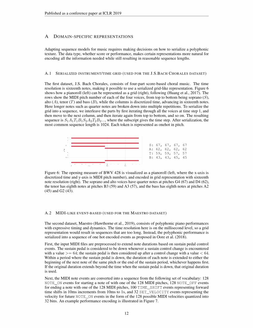
A.2 MIDI-LIKE EVENT-BASED (USED FOR THE MAESTRO DATASET)

The second dataset, Maestro (Hawthorne et al., 2019), consists of polyphonic piano performanceswith expressive timing and dynamics. The time resolution here is on the millisecond level, so a gridrepresentation would result in sequences that are too long. Instead, the polyphonic performance isserialized into a sequence of one hot encoded events as proposed in Oore et al. (2018).

First, the input MIDI files are preprocessed to extend note durations based on sustain pedal controlevents. The sustain pedal is considered to be down whenever a sustain control change is encounteredwith a value >= 64; the sustain pedal is then considered up after a control change with a value < 64.Within a period where the sustain pedal is down, the duration of each note is extended to either thebeginning of the next note of the same pitch or the end of the sustain period, whichever happens first.If the original duration extends beyond the time when the sustain pedal is down, that original durationis used.

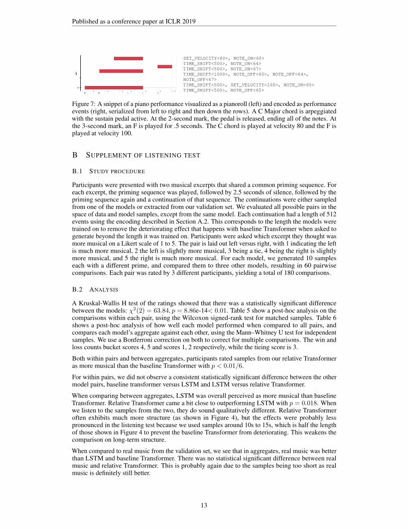
Next, the MIDI note events are converted into a sequence from the following set of vocabulary: 128NOTE_ON events for starting a note of with one of the 128 MIDI pitches, 128 NOTE_OFF eventsfor ending a note with one of the 128 MIDI pitches, 100 TIME_SHIFT events representing forwardtime shifts in 10ms increments from 10ms to 1s, and 32 SET_VELOCITY events representing thevelocity for future NOTE_ON events in the form of the 128 possible MIDI velocities quantized into32 bins. An example performance encoding is illustrated in Figure 7.

12


SET_VELOCITY<80>, NOTE_ON<60>TIME_SHIFT<500>, NOTE_ON<64>TIME_SHIFT<500>, NOTE_ON<67>TIME_SHIFT<1000>, NOTE_OFF<60>, NOTE_OFF<64>,NOTE_OFF<67>TIME_SHIFT<500>, SET_VELOCITY<100>, NOTE_ON<65>TIME_SHIFT<500>, NOTE_OFF<65>

Figure 7: A snippet of a piano performance visualized as a pianoroll (left) and encoded as performanceevents (right, serialized from left to right and then down the rows). A C Major chord is arpeggiatedwith the sustain pedal active. At the 2-second mark, the pedal is released, ending all of the notes. Atthe 3-second mark, an F is played for .5 seconds. The C chord is played at velocity 80 and the F isplayed at velocity 100.

B SUPPLEMENT OF LISTENING TEST

B.1 STUDY PROCEDURE

Participants were presented with two musical excerpts that shared a common priming sequence. Foreach excerpt, the priming sequence was played, followed by 2.5 seconds of silence, followed by thepriming sequence again and a continuation of that sequence. The continuations were either sampledfrom one of the models or extracted from our validation set. We evaluated all possible pairs in thespace of data and model samples, except from the same model. Each continuation had a length of 512events using the encoding described in Section A.2. This corresponds to the length the models weretrained on to remove the deteriorating effect that happens with baseline Transformer when asked togenerate beyond the length it was trained on. Participants were asked which excerpt they thought wasmore musical on a Likert scale of 1 to 5. The pair is laid out left versus right, with 1 indicating the leftis much more musical, 2 the left is slightly more musical, 3 being a tie, 4 being the right is slightlymore musical, and 5 the right is much more musical. For each model, we generated 10 sampleseach with a different prime, and compared them to three other models, resulting in 60 pairwisecomparisons. Each pair was rated by 3 different participants, yielding a total of 180 comparisons.

B.2 ANALYSIS

A Kruskal-Wallis H test of the ratings showed that there was a statistically significant differencebetween the models: χ2(2) = 63.84, p = 8.86e-14< 0.01. Table 5 show a post-hoc analysis on thecomparisons within each pair, using the Wilcoxon signed-rank test for matched samples. Table 6shows a post-hoc analysis of how well each model performed when compared to all pairs, andcompares each model’s aggregate against each other, using the Mann–Whitney U test for independentsamples. We use a Bonferroni correction on both to correct for multiple comparisons. The win andloss counts bucket scores 4, 5 and scores 1, 2 respectively, while the tieing score is 3.

Both within pairs and between aggregates, participants rated samples from our relative Transformeras more musical than the baseline Transformer with p < 0.01/6.

For within pairs, we did not observe a consistent statistically significant difference between the othermodel pairs, baseline transformer versus LSTM and LSTM versus relative Transformer.

When comparing between aggregates, LSTM was overall perceived as more musical than baselineTransformer. Relative Transformer came a bit close to outperforming LSTM with p = 0.018. Whenwe listen to the samples from the two, they do sound qualitatively different. Relative Transformeroften exhibits much more structure (as shown in Figure 4), but the effects were probably lesspronounced in the listening test because we used samples around 10s to 15s, which is half the lengthof those shown in Figure 4 to prevent the baseline Transformer from deteriorating. This weakens thecomparison on long-term structure.

When compared to real music from the validation set, we see that in aggregates, real music was betterthan LSTM and baseline Transformer. There was no statistical significant difference between realmusic and relative Transformer. This is probably again due to the samples being too short as realmusic is definitely still better.

13


Table 5: A post-hoc comparison of each pair on their pairwise comparisons with each other, using theWilcoxon signed-rank test for matched samples. p value less than 0.01/6=0.0016 yields a statisticallysignificant difference and is marked by asterisk.

Pairs wins ties losses p value

Our relative transformer real music 11 4 15 0.243Our relative transformer Baseline transformer 23 1 6 0.0006*Our relative transformer LSTM 18 1 11 0.204Baseline transformer LSTM 5 3 22 0.006Baseline transformer real music 6 0 24 0.0004*LSTM real music 6 2 22 0.0014

Table 6: Comparing each pair on their aggregates (comparisons with all models) in (wins, ties, losses),using the Mann–Whitney U test for independent samples.

Model Model p value

Our relative transformer (52, 6, 32) real music (61, 6, 23) 0.020Our relative transformer (52, 6, 32) Baseline transformer (17, 4, 69) 1.26e-9*Our relative transformer (52, 6, 32) LSTM (39, 6, 45) 0.018Baseline transformer (17, 4, 69) LSTM (39, 6, 45) 3.70e-5*Baseline transformer (17, 4, 69) real music (61, 6, 23) 6.73e-14*LSTM (39, 6, 45) real music (61, 6, 23) 4.06e-5*

C VISUALIZING SOFTMAX ATTENTION

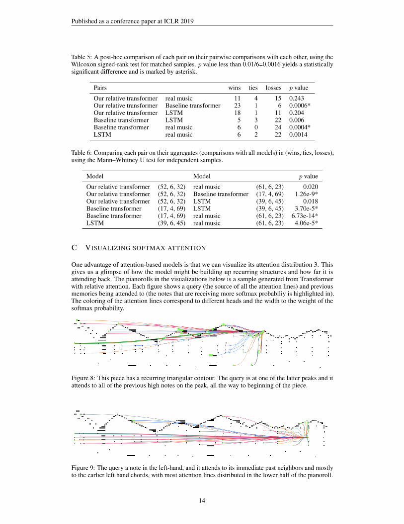
One advantage of attention-based models is that we can visualize its attention distribution 3. Thisgives us a glimpse of how the model might be building up recurring structures and how far it isattending back. The pianorolls in the visualizations below is a sample generated from Transformerwith relative attention. Each figure shows a query (the source of all the attention lines) and previousmemories being attended to (the notes that are receiving more softmax probabiliy is highlighted in).The coloring of the attention lines correspond to different heads and the width to the weight of thesoftmax probability.

Figure 8: This piece has a recurring triangular contour. The query is at one of the latter peaks and itattends to all of the previous high notes on the peak, all the way to beginning of the piece.

Figure 9: The query a note in the left-hand, and it attends to its immediate past neighbors and mostlyto the earlier left hand chords, with most attention lines distributed in the lower half of the pianoroll.

14


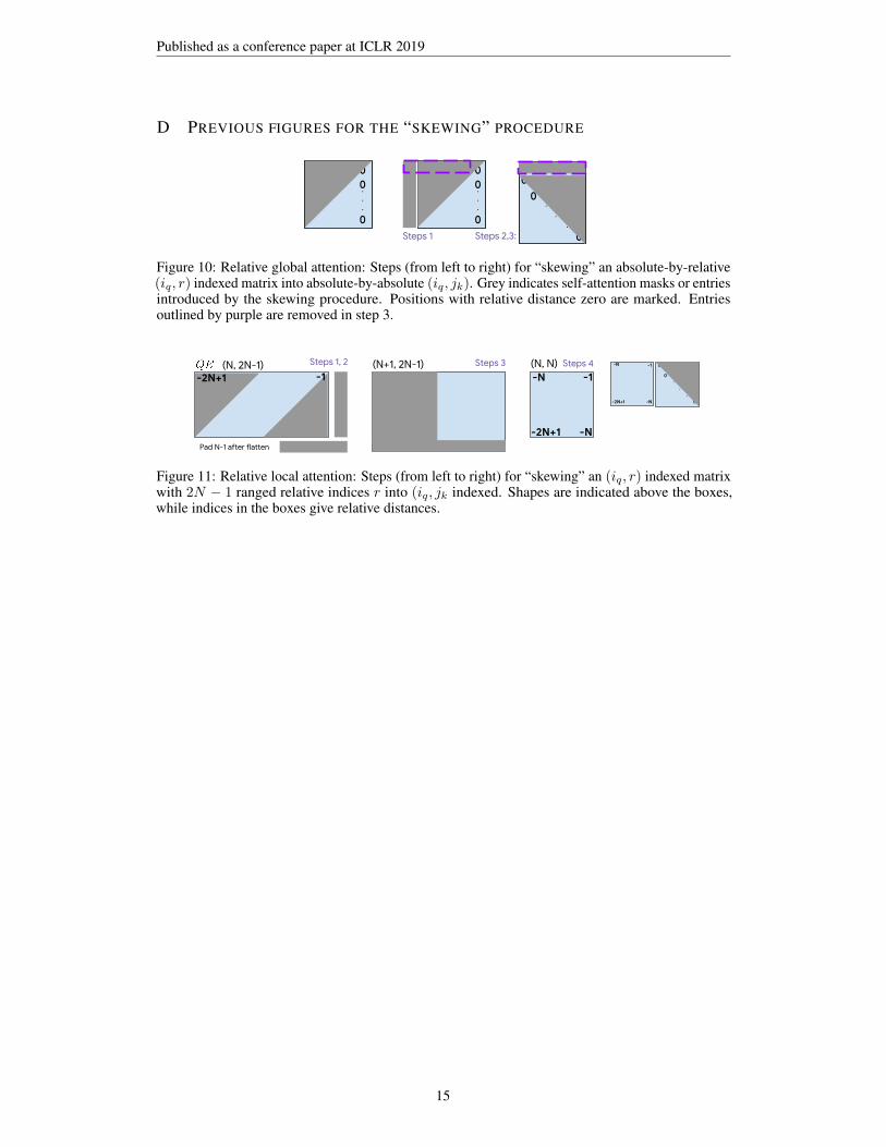
D PREVIOUS FIGURES FOR THE “SKEWING” PROCEDURE

00...

0

00...

0

00

0

..

.

Steps 1 Steps 2,3:

Figure 10: Relative global attention: Steps (from left to right) for “skewing” an absolute-by-relative(iq, r) indexed matrix into absolute-by-absolute (iq, jk). Grey indicates self-attention masks or entriesintroduced by the skewing procedure. Positions with relative distance zero are marked. Entriesoutlined by purple are removed in step 3.

(N+1, 2N-1)-1

-N-2N+1

-N(N, N)

0

0

0

..

.

-1

-N-2N+1

-N

-1-2N+1(N, 2N-1)

Pad N-1 after flatten

Steps 1, 2 Steps 3 Steps 4

Figure 11: Relative local attention: Steps (from left to right) for “skewing” an (iq, r) indexed matrixwith 2N − 1 ranged relative indices r into (iq, jk indexed. Shapes are indicated above the boxes,while indices in the boxes give relative distances.

15

MUSIC TRANSFORMER GENERATING MUSIC WITH LONG TERM …

Documents

Transcript of MUSIC TRANSFORMER GENERATING MUSIC WITH LONG TERM …