Module 10 July 22, 2014 - University of North Carolina at...
108
1 15 Module 10 July 22, 2014
Transcript of Module 10 July 22, 2014 - University of North Carolina at...

1
15
Module 10
July 22, 2014

Production Planning Process
Process Planning
Strategic Capacity Planning
Aggregate Planning
Long
Range
Medium
Range
Short
Range
How much & when
to produce
Aggregate Production Planning/ Sales and Operations Planning (S&OP)
• A managerial statement of time-phased
–production rates,
–work-force levels, and
– inventory investment,
which takes into account customer requirements and capacity limitations

Aggregate Production Planning Sales and Operations Planning (S&OP)
• Objective:
Generally to determine the quantity and timing of production for the intermediate future (generally 6 - 18 months); called the “planning horizon.”
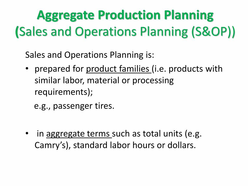
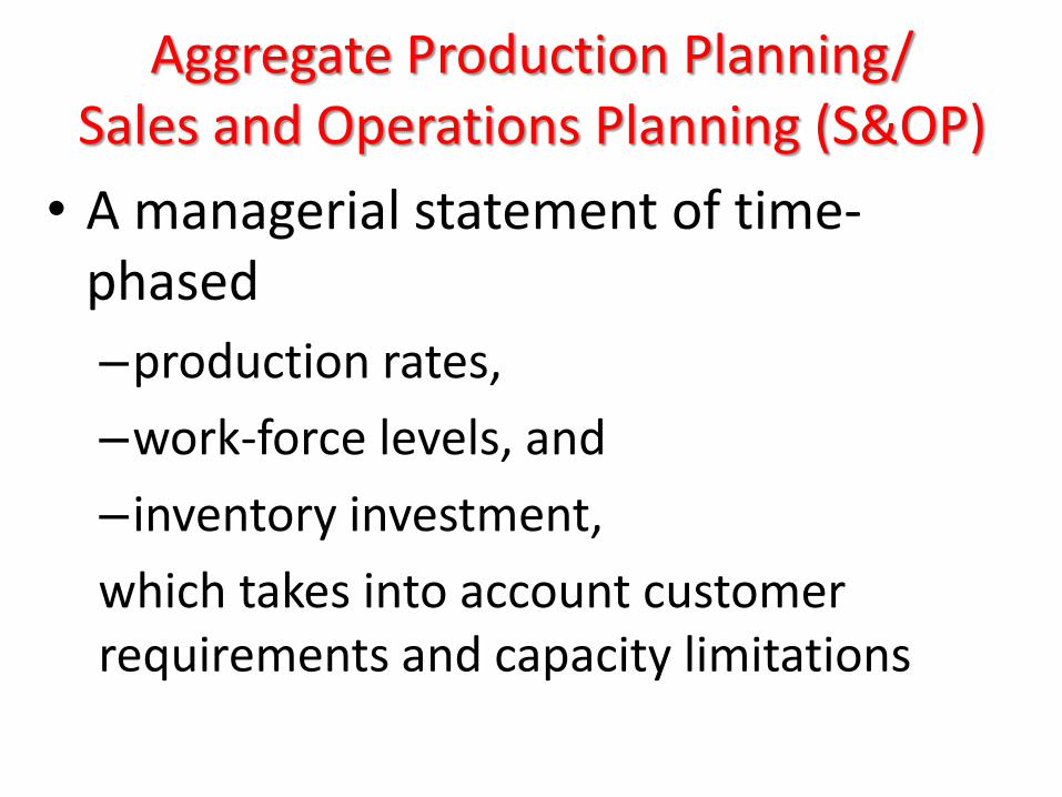
Aggregate Production Planning (Sales and Operations Planning (S&OP))
Sales and Operations Planning is:
• prepared for product families (i.e. products with similar labor, material or processing requirements);
e.g., passenger tires.
• in aggregate terms such as total units (e.g. Camry’s), standard labor hours or dollars.
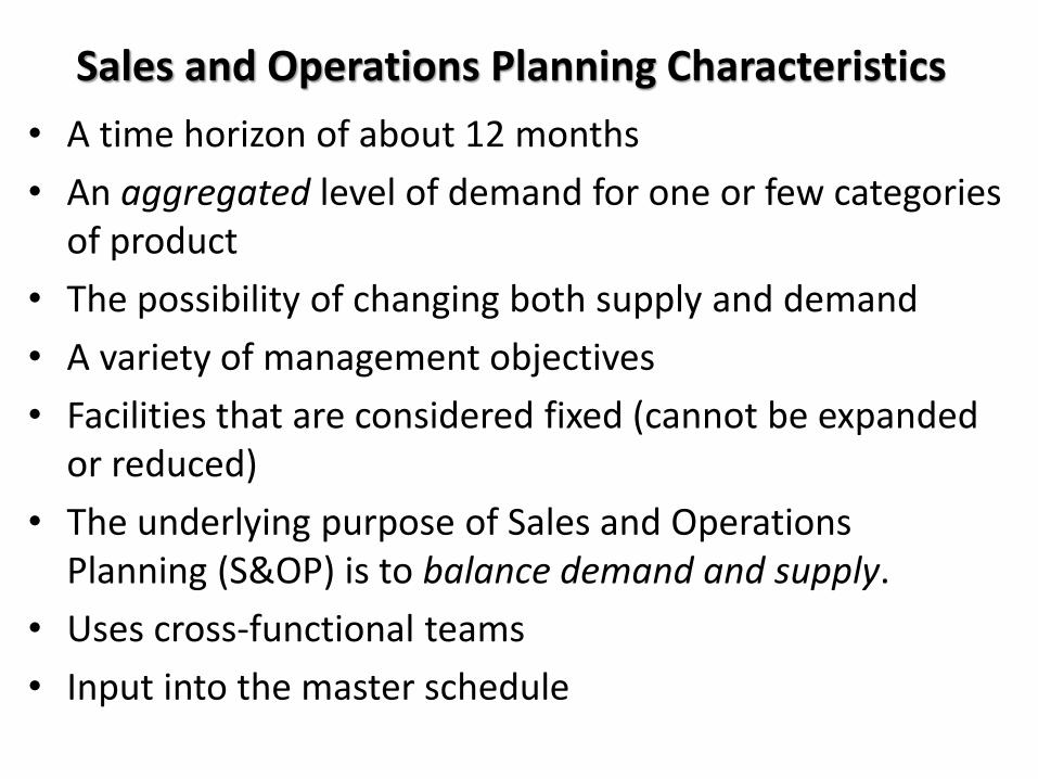
Sales and Operations Planning Characteristics
• A time horizon of about 12 months
• An aggregated level of demand for one or few categories of product
• The possibility of changing both supply and demand
• A variety of management objectives
• Facilities that are considered fixed (cannot be expanded or reduced)
• The underlying purpose of Sales and Operations Planning (S&OP) is to balance demand and supply.
• Uses cross-functional teams
• Input into the master schedule

The Balancing Act
Demand Supply
Sales
Forecasts Actual
Orders
Production
Orders
Purchase
Orders
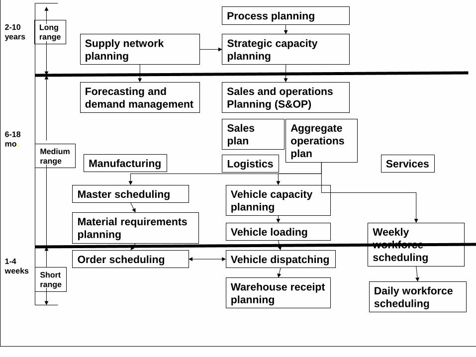
Process planning
Strategic capacity
planning
Sales and operations
Planning (S&OP)
Sales
plan
Aggregate
operations
plan
Supply network
planning
Forecasting and
demand management
Master scheduling
Material requirements
planning
Order scheduling
Vehicle capacity
planning
Vehicle loading
Vehicle dispatching
Warehouse receipt
planning
Weekly
workforce
scheduling
Daily workforce
scheduling
Manufacturing Logistics Services
Long
range
Medium
range
Short
range
2-10
years
6-18
mo.
1-4
weeks

Planning for Production (Old)
Sales
Planning
Aggregate
Planning
Master
Scheduling
Detailed Planning
& Scheduling
C
A
P
A
C
I
T
Y
P
L
A
N
N
I
N
G
F
O
R
E
C
A
S
T
I
N
G
&
D
E
M
A
N
D
Business
Planning
Source: Wallace, Tom F. Sales and Operations Planning, A How-To Guide, T.F. Wallace & Co. 1999.
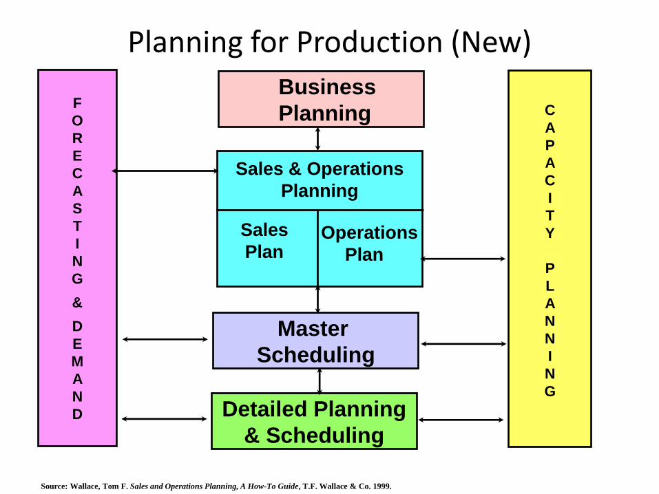
Planning for Production (New)
Sales & Operations
Planning
Master
Scheduling
Detailed Planning
& Scheduling
C
A
P
A
C
I
T
Y
P
L
A
N
N
I
N
G
F
O
R
E
C
A
S
T
I
N
G
&
D
E
M
A
N
D
Business
Planning
Sales
Plan Operations
Plan
Source: Wallace, Tom F. Sales and Operations Planning, A How-To Guide, T.F. Wallace & Co. 1999.

Planning Options
• Options for managing demand.
– influencing demand from customers
–delivering orders as promised
• Options for managing supply
–delivering what is promised
–managing capacity & other resources

Options for Influencing (Managing) Demand
• Pricing
• Advertising and promotion
• Backlog or reservations (shifting demand)
• Development of complementary products

Demand Management
Influencing What the Customer will Buy

Demand Management
Influencing What the Customer will Buy

Options for Influencing (managing) Supply
• Hiring and layoff of employees
• Using overtime and under-time
• Using part-time or temporary labor
• Carrying inventory
• Outsourcing or Subcontracting
• Making cooperative arrangements

Outsourcing or Subcontracting
Using someone else’s capacity to
help manage supply

Outsourcing or Subcontracting
Using
someone
else’s
capacity
to help
manage
supply
Outsourcing or Subcontracting
Using someone else’s capacity to
help manage supply

S&OP: Who Brings What to the Table?
Marketing Product
Definition
Product
Demand
Capital
Master
Schedule
Business
Plan
Workforce
Availability
Source: Launchbury, Keith J. Principles of Planning Omeric, 1999.
Finance
Materials Operations
Human
Resources
Engineering
Management
Capacity

Inputs to S&OP •Input Responsibility
•Demand Forecast Marketing
•Market intelligence Marketing
•Actual sales Sales
•Capacity information Manufacturing
•Management targets Management
•Financial requirements Finance
•New product information R&D
•New process information Process engineering
•Workforce availability Human resources

Sales and Operations Planning
Specific Inputs needed are:
• updated sales forecast for the planning horizon
• company policies on acceptable inventory levels, personnel
(e.g., no backordering, no layoffs, overtime up to 20% of
• regular time, etc.), subcontracting and others
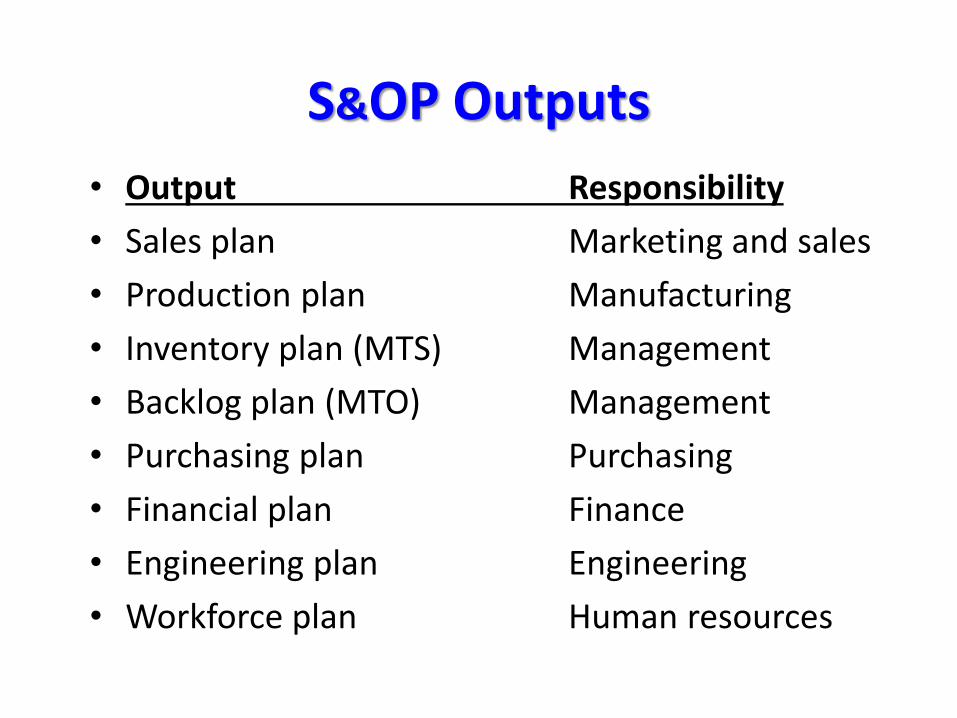
S&OP Outputs
• Output Responsibility
• Sales plan Marketing and sales
• Production plan Manufacturing
• Inventory plan (MTS) Management
• Backlog plan (MTO) Management
• Purchasing plan Purchasing
• Financial plan Finance
• Engineering plan Engineering
• Workforce plan Human resources

Inputs and Outputs of S & OP
Demand
Capacity Constraint
Company Policies
Amount of product
subcontracted and backordered
Size of work force
Inventory Levels
Production per month
Sales and Operations Planning

Iterative Nature of S&OP
1. Develop production plan.
2. Check implications for inventory/backlog plan.
3. If necessary, adjust production plan.
4. Check against resource plan and availability.
5. If necessary, adjust production plan.
6. Recheck against inventory/backlog and
resources.
7. Continue (go to 5) until you meet all constraints.

Sales and Operations Planning
Criteria generally used include:
• Minimizing cost
• Maximizing customer service level
• Minimizing inventory
• Maintaining a stable work force level
• Combination of the above

Methods for Sales and Operations Planning
• Intuitive approach
• Analytical approaches – – Transportation method of linear programming
– Linear Decision Rule (LDR),
– Management Coefficients Model (MCM),
– Parametric Production Planning (PPP),
– Search Decision Rule (SDR), etc.
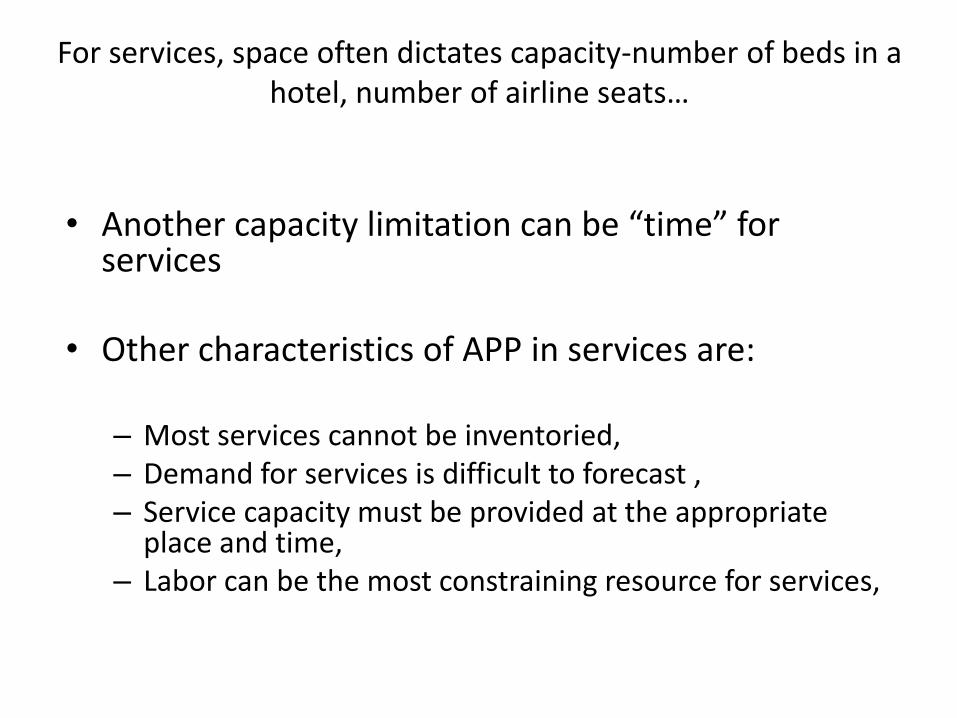
For services, space often dictates capacity-number of beds in a hotel, number of airline seats…
• Another capacity limitation can be “time” for
services
• Other characteristics of APP in services are:
– Most services cannot be inventoried, – Demand for services is difficult to forecast , – Service capacity must be provided at the appropriate
place and time, – Labor can be the most constraining resource for services,

The following are common Sales and Operations Planning choices within different strategies
• Inventories are used to absorb demand.
• Over time and under time can be used to increase or decrease production.
• Subcontracting can be used.
• Part-time workers can be used.

Important cost factors
• Regular production cost
• Over time cost.
• Subcontracting cost.

Important cost factors
• Inventory holding cost
• Backordering cost
• Hiring cost
• Layoff cost

Alternative approaches - or how to reduce the need for Sales and Operations
planning
• Use substitute or alternative products
• Promotional campaigns
• Creative pricing
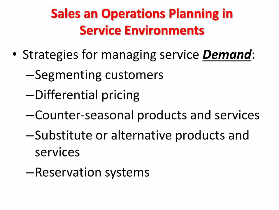
Sales an Operations Planning in Service Environments
• Strategies for managing service Demand:
–Segmenting customers
–Differential pricing
–Counter-seasonal products and services
–Substitute or alternative products and services
–Reservation systems
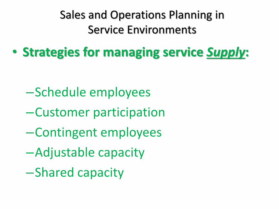
Sales and Operations Planning in Service Environments
• Strategies for managing service Supply:
–Schedule employees
–Customer participation
–Contingent employees
–Adjustable capacity
–Shared capacity

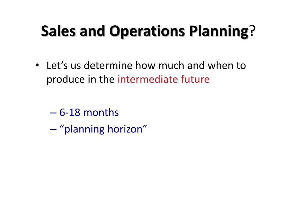
Sales and Operations Planning?
• Let’s us determine how much and when to produce in the intermediate future
– Examples
• labor hours of production
• total number of units (in aggregate) – # of cars to make
NOT
# of red cars,
# of green cars,
# of 2-doors,…

Sales and Operations Planning?
• Let’s us determine how much and when to produce in the intermediate future
– which periods (months, quarters, etc.)?
Sales and Operations Planning?
• Let’s us determine how much and when to produce in the intermediate future
– 6-18 months
– “planning horizon”

Sales and Operations Planning?
• Let’s us determine how much and when to produce in the intermediate future
• Goal
– Minimize the cost of resources required to meet demand over the planning horizon
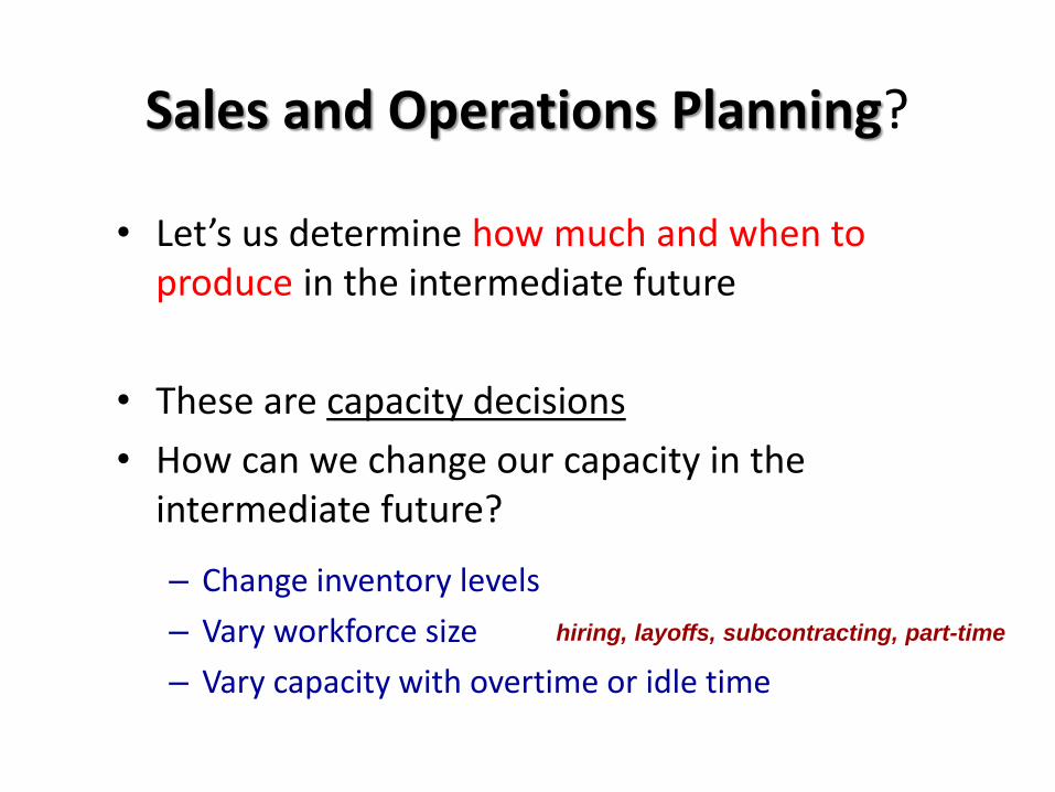
Sales and Operations Planning?
• Let’s us determine how much and when to produce in the intermediate future
• These are capacity decisions
• How can we change our capacity in the intermediate future?
– Change inventory levels
– Vary workforce size
– Vary capacity with overtime or idle time
hiring, layoffs, subcontracting, part-time

Basic Production Strategies
• “Level” strategy (constant work
force, use inventory as buffer)
• “Chase” strategy (produce to
demand, vary workforce)

Level Strategy
• Deliver products and services at a constant rate
• Avoid making changes to operations

Level Production Strategy
J F M A M J J A S O N D
Time
Dem
and
Demand
Production
Reprinted with permission, J.R. Tony Arnold, Introduction to Materials Management, third edition, Prentice-Hall,
1998

Level Production Strategy (cont.)
• Advantage:
– Smooth, level production avoids labor costs of demand matching
• Disadvantage:
– Buildup of inventory
– Requires accurate forecast

Chase Strategy
• Produce only what you sell
• Produce products or services just-in-time
• If there are no sales—do not produce
• Typical for services

Chase Strategy

Chase Strategy • Advantages:
– Stable inventory
– Varied production to meet sales requirements
• Disadvantages:
– Costs of hiring, training, overtime, and extra shifts
– Costs of layoffs and impact on employee morale
– Possible unavailability of needed work skills
– Maximum capacity needed

Sales and Operations Planning Costs
• Hiring and firing costs (chase)
• Overtime and under-time costs (chase)
• Subcontracting costs (chase)
• Part-time labor costs (chase)
• Inventory-carrying costs (level)
• Cost of stockout or back order (level)

Combination Strategy
J F M A M J J A S O N D
Time
Dem
and
Demand
Production
Reprinted with permission, J.R. Tony Arnold, Introduction to Materials Management, third edition, Prentice-Hall,
1998

Combination Strategy (cont.)
– Produces at or close to full capacity for some part of the cycle
– Produces at a lower rate (or does not produce) during the rest of the cycle
– Makes use of available capacity, yet limits inventory buildup and inventory carrying costs

Minimum Production Strategy

Minimum Strategy (cont.)
– Produces at or close to full capacity for all of the cycle
– Subcontracts for demand above the minimum
– Makes full use of available capacity, and eliminates inventory buildup and inventory carrying costs

Comparison of Chase versus Level Strategy
Chase
Demand
Level
CapacityLevel of labor skill required Low High
Job discretion Low High
Compensation rate Low High
Training required per employee Low High
Labor turnover High Low
Hire-fire cost High Low
Error rate High Low
Amount of supervision required High Low
Type of budgeting and forecasting required Short-run Long-run
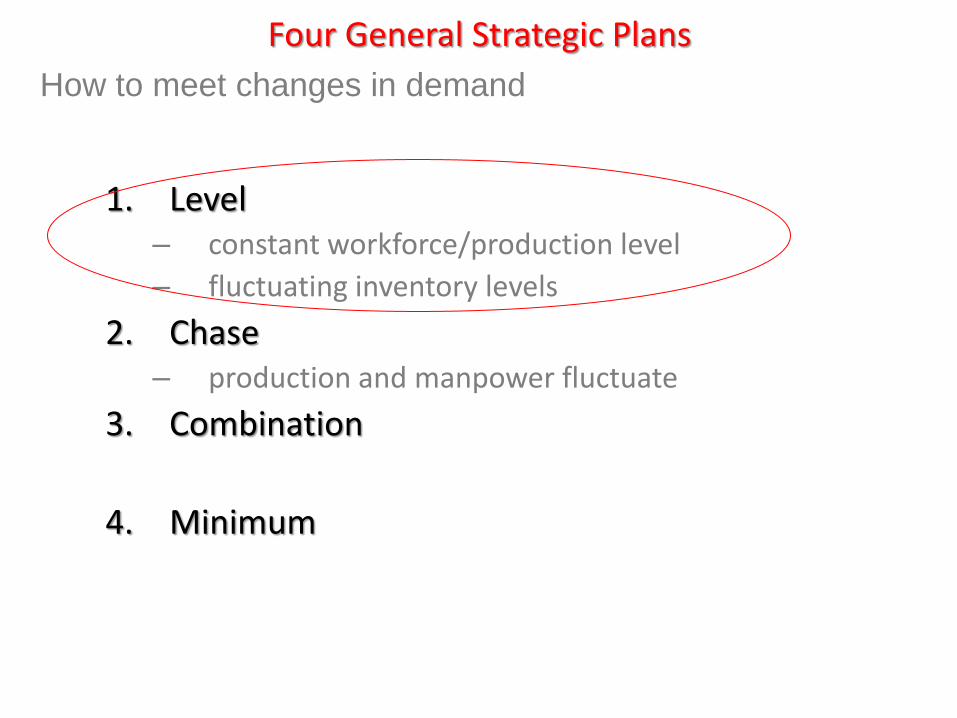
Four General Strategic Plans
1. Level – constant workforce/production level
– fluctuating inventory levels
2. Chase – production and manpower fluctuate
3. Combination
4. Minimum
How to meet changes in demand

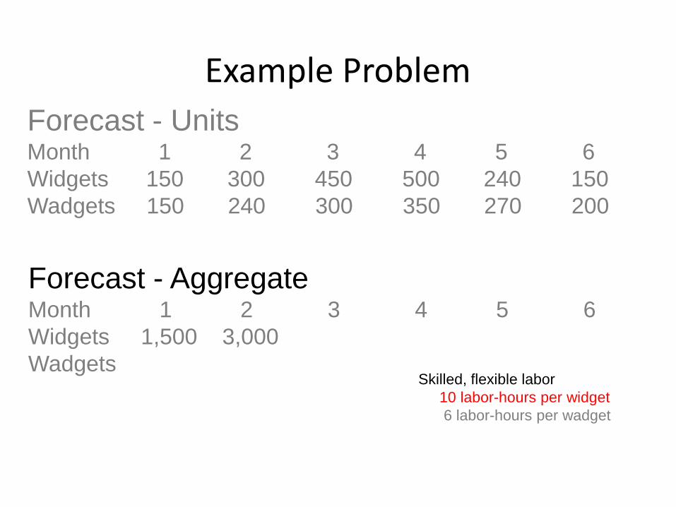
Example Problem
Forecast - Units Month 1 2 3 4 5 6
Widgets 150 300 450 500 240 150
Wadgets 150 240 300 350 270 200
Skilled, flexible labor
10 labor-hours per widget
6 labor-hours per wadget

Example Problem
Forecast - Units Month 1 2 3 4 5 6
Widgets 150 300 450 500 240 150
Wadgets 150 240 300 350 270 200
Skilled, flexible labor
10 labor-hours per widget
6 labor-hours per wadget
Forecast - Aggregate Month 1 2 3 4 5 6
Widgets
Wadgets

Example Problem
Forecast - Units Month 1 2 3 4 5 6
Widgets 150 300 450 500 240 150
Wadgets 150 240 300 350 270 200
Skilled, flexible labor
10 labor-hours per widget
6 labor-hours per wadget
Forecast - Aggregate Month 1 2 3 4 5 6
Widgets 1,500
Wadgets
Example Problem
Forecast - Units Month 1 2 3 4 5 6
Widgets 150 300 450 500 240 150
Wadgets 150 240 300 350 270 200
Skilled, flexible labor
10 labor-hours per widget
6 labor-hours per wadget
Forecast - Aggregate Month 1 2 3 4 5 6
Widgets 1,500 3,000
Wadgets

Example Problem
Forecast - Units Month 1 2 3 4 5 6
Widgets 150 300 450 500 240 150
Wadgets 150 240 300 350 270 200
Skilled, flexible labor
10 labor-hours per widget
6 labor-hours per wadget
Forecast - Aggregate Month 1 2 3 4 5 6
Widgets 1,500 3,000 4,500
Wadgets

Example Problem
Forecast - Units Month 1 2 3 4 5 6
Widgets 150 300 450 500 240 150
Wadgets 150 240 300 350 270 200
Skilled, flexible labor
10 labor-hours per widget
6 labor-hours per wadget
Forecast - Aggregate Month 1 2 3 4 5 6
Widgets 1,500 3,000 4,500 5,000
Wadgets

Example Problem
Forecast - Units Month 1 2 3 4 5 6
Widgets 150 300 450 500 240 150
Wadgets 150 240 300 350 270 200
Skilled, flexible labor
10 labor-hours per widget
6 labor-hours per wadget
Forecast - Aggregate Month 1 2 3 4 5 6
Widgets 1,500 3,000 4,500 5,000 2,400
Wadgets

Example Problem
Forecast - Units Month 1 2 3 4 5 6
Widgets 150 300 450 500 240 150
Wadgets 150 240 300 350 270 200
Skilled, flexible labor
10 labor-hours per widget
6 labor-hours per wadget
Forecast - Aggregate Month 1 2 3 4 5 6
Widgets 1,500 3,000 4,500 5,000 2,400 1,500
Wadgets

Example Problem
Forecast - Units Month 1 2 3 4 5 6
Widgets 150 300 450 500 240 150
Wadgets 150 240 300 350 270 200
Skilled, flexible labor
10 labor-hours per widget
6 labor-hours per wadget
Forecast - Aggregate Month 1 2 3 4 5 6
Widgets 1,500 3,000 4,500 5,000 2,400 1,500
Wadgets

Example Problem
Forecast - Units Month 1 2 3 4 5 6
Widgets 150 300 450 500 240 150
Wadgets 150 240 300 350 270 200
Skilled, flexible labor
10 labor-hours per widget
6 labor-hours per wadget
Forecast - Aggregate Month 1 2 3 4 5 6
Widgets 1,500 3,000 4,500 5,000 2,400 1,500
Wadgets 900

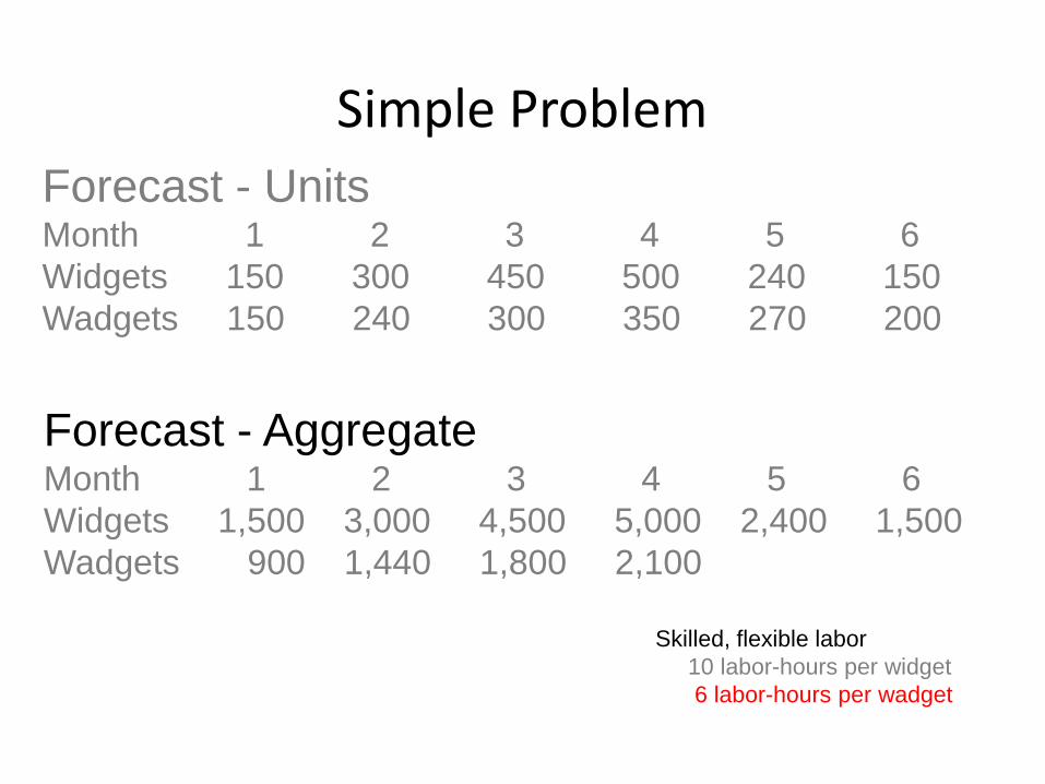
Simple Problem
Forecast - Units Month 1 2 3 4 5 6
Widgets 150 300 450 500 240 150
Wadgets 150 240 300 350 270 200
Skilled, flexible labor
10 labor-hours per widget
6 labor-hours per wadget
Forecast - Aggregate Month 1 2 3 4 5 6
Widgets 1,500 3,000 4,500 5,000 2,400 1,500
Wadgets 900 1,440

Simple Problem
Forecast - Units Month 1 2 3 4 5 6
Widgets 150 300 450 500 240 150
Wadgets 150 240 300 350 270 200
Skilled, flexible labor
10 labor-hours per widget
6 labor-hours per wadget
Forecast - Aggregate Month 1 2 3 4 5 6
Widgets 1,500 3,000 4,500 5,000 2,400 1,500
Wadgets 900 1,440 1,800
Simple Problem
Forecast - Units Month 1 2 3 4 5 6
Widgets 150 300 450 500 240 150
Wadgets 150 240 300 350 270 200
Skilled, flexible labor
10 labor-hours per widget
6 labor-hours per wadget
Forecast - Aggregate Month 1 2 3 4 5 6
Widgets 1,500 3,000 4,500 5,000 2,400 1,500
Wadgets 900 1,440 1,800 2,100

Example Problem
Forecast - Units Month 1 2 3 4 5 6
Widgets 150 300 450 500 240 150
Wadgets 150 240 300 350 270 200
Skilled, flexible labor
10 labor-hours per widget
6 labor-hours per wadget
Forecast - Aggregate Month 1 2 3 4 5 6
Widgets 1,500 3,000 4,500 5,000 2,400 1,500
Wadgets 900 1,440 1,800 2,100 1,620
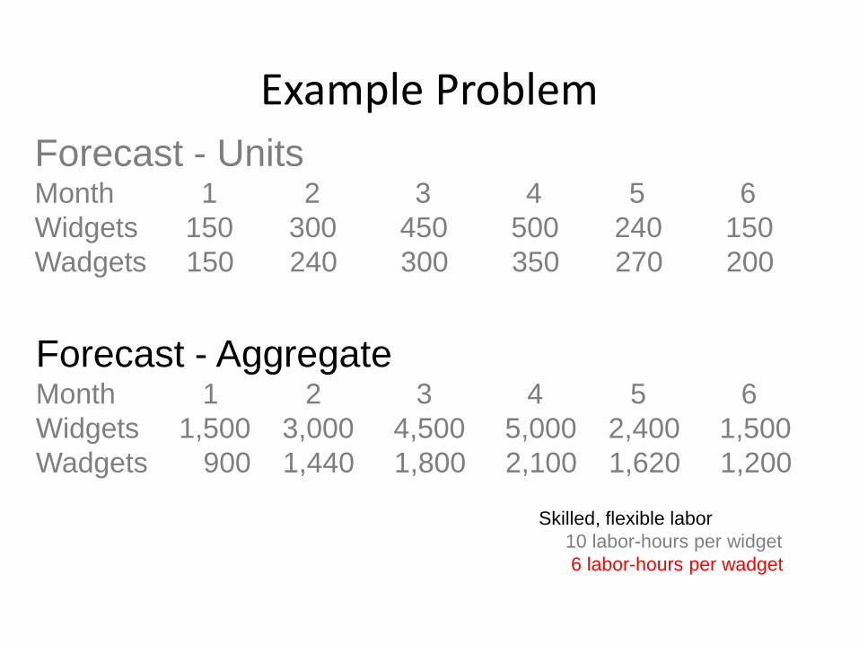
Example Problem
Forecast - Units Month 1 2 3 4 5 6
Widgets 150 300 450 500 240 150
Wadgets 150 240 300 350 270 200
Skilled, flexible labor
10 labor-hours per widget
6 labor-hours per wadget
Forecast - Aggregate Month 1 2 3 4 5 6
Widgets 1,500 3,000 4,500 5,000 2,400 1,500
Wadgets 900 1,440 1,800 2,100 1,620 1,200
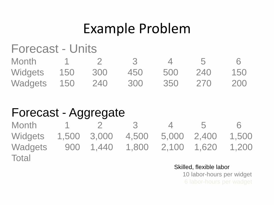
Total

Example Problem
Forecast - Units Month 1 2 3 4 5 6
Widgets 150 300 450 500 240 150
Wadgets 150 240 300 350 270 200
Forecast - Aggregate Month 1 2 3 4 5 6
Widgets 1,500 3,000 4,500 5,000 2,400 1,500
Wadgets 900 1,440 1,800 2,100 1,620 1,200
Total 2,400 4,440 6,300 7,100 4,020 2,700
Cumul

Example Problem
Forecast - Units Month 1 2 3 4 5 6
Widgets 150 300 450 500 240 150
Wadgets 150 240 300 350 270 200
Forecast - Aggregate Month 1 2 3 4 5 6
Widgets 1,500 3,000 4,500 5,000 2,400 1,500
Wadgets 900 1,440 1,800 2,100 1,620 1,200
Total 2,400 4,440 6,300 7,100 4,020 2,700
Cumul 2,400 6,840 13,140 20,240 24,260 26,960

Simple Problem
Forecast - Aggregate Month 1 2 3 4 5 6
Widgets 1,500 3,000 4,500 5,000 2,400 1,500
Wadgets 900 1,440 1,800 2,100 1,620 1,200
Total 2,400 4,440 6,300 7,100 4,020 2,700
Cumul 2,400 6,840 13,140 20,240 24,260 26,960

Simple Problem
• Basic equation
– Ending Inventory =
Forecast - Aggregate Month 1 2 3 4 5 6
Widgets 1,500 3,000 4,500 5,000 2,400 1,500
Wadgets 900 1,440 1,800 2,100 1,620 1,200
Total 2,400 4,440 6,300 7,100 4,020 2,700
Cumul 2,400 6,840 13,140 20,240 24,260 26,960
Beginning + Production - Demand
Inventory
What is left over = what you
begin with
+ what came in - what went
out
Example Problem
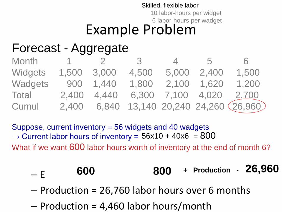
– Ending Inventory =
– Production = 26,760 labor hours over 6 months
– Production = 4,460 labor hours/month
Skilled, flexible labor
10 labor-hours per widget
6 labor-hours per wadget
Forecast - Aggregate Month 1 2 3 4 5 6
Widgets 1,500 3,000 4,500 5,000 2,400 1,500
Wadgets 900 1,440 1,800 2,100 1,620 1,200
Total 2,400 4,440 6,300 7,100 4,020 2,700
Cumul 2,400 6,840 13,140 20,240 24,260 26,960
Suppose, current inventory = 56 widgets and 40 wadgets
→ Current labor hours of inventory =
What if we want 600 labor hours worth of inventory at the end of month 6?
Beginning + Production - Demand
Inventory 600
800
26,960
56x10 + 40x6 = 800

Level Plan With Backorders
– Production = 4,460 labor hours/month
Month 1 2 3 4 5 6
BI
Demand 2,400 4,440 6,300 7,100 4,020 2,700
Prod. 4,460 4,460 4,460 4,460 4,460 4,460
EI
→ Current labor hours of inventory = 56x10 + 40x6 = 800
What if we want 600 labor hours worth of inventory at the end of month 6?
800
600
DEMANDS FROM
THE PREVIOUS SLIDE
Demand
4,460

Level Plan With Backorders
– Ending Inventory =
– Production = 4,460 labor hours/month
Month 1 2 3 4 5 6
BI
Demand 2,400 4,440 6,300 7,100 4,020 2,700
Prod. 4,460 4,460 4,460 4,460 4,460 4,460
EI
2,860 2,880
2,860 2,880
1,040
1,040
(1,600)
(1,600)
(1,160)
(1,160) 800
600
Values in parenthesis are negative,
representing backorders
Beginning + Production - Demand
Inventory …what if we don’t want
to permit backorders?

Level Plan Without Backorders
• Level plan with minimum inventory and no backorders
• Key point: in one of six months ending inventory will be zero – If it never falls to zero, we are keeping more inventory
than needed
• Solution: solve 6 level plans – Each plan has zero ending inventory in one of the six
months
– Highest production level is solution

Solved problem
Month 1 2 3 4 5 6
BI 800 3,260 3,680 2,240 0 840
Demand 2,400 4,440 6,300 7,100 4,020 2,700
Prod. 4,860 4,860 4,860 4,860 4,860 4,860
EI 3,260 3,680 2,240 0 840 3,000

Solved problem
Month 1 2 3 4 5 6
BI 800 3,260 3,680 2,240 0 840
Demand 2,400 4,440 6,300 7,100 4,020 2,700
Prod. 4,860 4,860 4,860 4,860 4,860 4,860
EI 3,260 3,680 2,240 0 840 3,000

Solved problem
Month 1 2 3 4 5 6
BI 800 3,260 3,680 2,240 0 840
Demand 2,400 4,440 6,300 7,100 4,020 2,700
Prod. 4,860 4,860 4,860 4,860 4,860 4,860
EI 3,260 3,680 2,240 0 840 3,000

Solved problem
Month 1 2 3 4 5 6
BI 800 3,260 3,680 2,240 0 840
Demand 2,400 4,440 6,300 7,100 4,020 2,700
Prod. 4,860 4,860 4,860 4,860 4,860 4,860
EI 3,260 3,680 2,240 0 840 3,000

Let’s extend this example
to look at the other strategies…
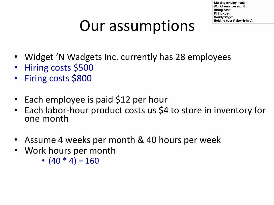
Our assumptions
• Widget ‘N Wadgets Inc. currently has 28 employees • Hiring costs $500 • Firing costs $800
• Each employee is paid $12 per hour • Each labor-hour product costs us $4 to store in inventory for
one month
• Assume 4 weeks per month & 40 hours per week • Work hours per month
• (40 * 4) = 160

Month 1 2 3 4 5 6 BI 800 3,260 3,680 2,240 0 840
Demand 2,400 4,440 6,300 7,100 4,020 2,700
Prod. 4,860 4,860 4,860 4,860 4,860 4,860
EI 3,260 3,680 2,240 0 840 3,000
From the previous example…
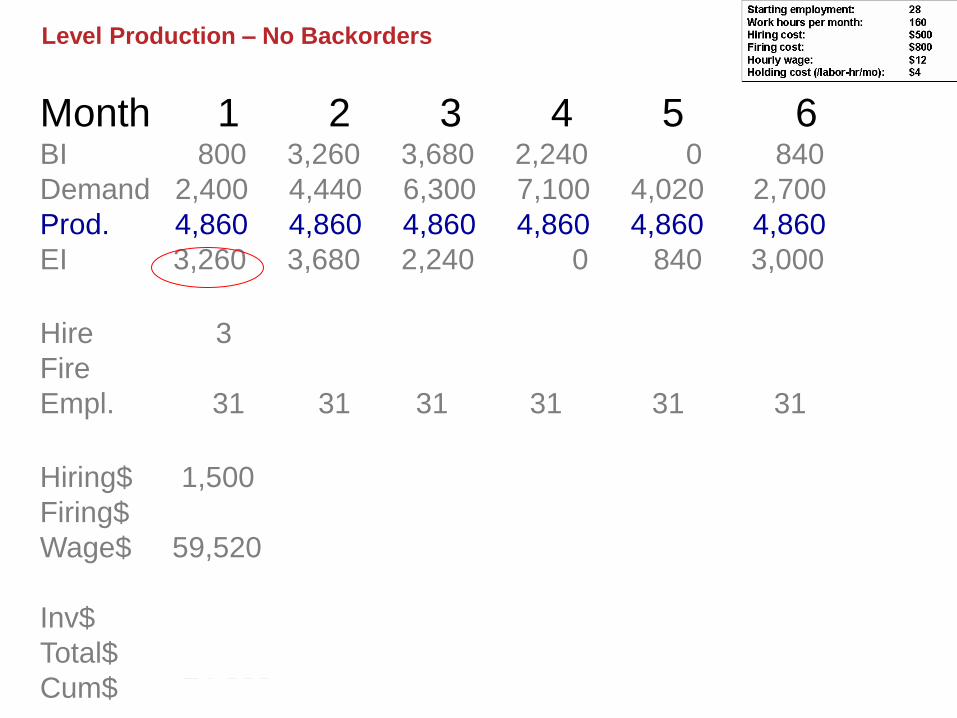
Level Production – No Backorders

Month 1 2 3 4 5 6 BI 800 3,260 3,680 2,240 0 840
Demand 2,400 4,440 6,300 7,100 4,020 2,700
Prod. 4,860 4,860 4,860 4,860 4,860 4,860
EI 3,260 3,680 2,240 0 840 3,000
Hire 3
Fire
Empl. 31 31 31 31 31 31
Hiring$ 1,500
Firing$
Wage$ 59,520 59,520 59,520 59,520 59,520 59,520
Inv$ 13,040 14,720 8,960 0 3,360 12,000
Total$ 74,060 74,240 68,480 59,520 62,880 71,520
Cum$ 74,060 148,300 216,780 276,300 339,180 410,700
Level Production – No Backorders
# workers
needed in
month 1
4860 hr/mo
160 hr/mo
1 worker
=30.375 = ~31 workers

Month 1 2 3 4 5 6 BI 800 3,260 3,680 2,240 0 840
Demand 2,400 4,440 6,300 7,100 4,020 2,700
Prod. 4,860 4,860 4,860 4,860 4,860 4,860
EI 3,260 3,680 2,240 0 840 3,000
Hire 3
Fire
Empl. 31 31 31 31 31 31
Hiring$ 1,500
Firing$
Wage$ 59,520 59,520 59,520 59,520 59,520 59,520
Inv$ 13,040 14,720 8,960 0 3,360 12,000
Total$ 74,060 74,240 68,480 59,520 62,880 71,520
Cum$ 74,060 148,300 216,780 276,300 339,180 410,700
Level Production – No Backorders
but we only have 28

Month 1 2 3 4 5 6 BI 800 3,260 3,680 2,240 0 840
Demand 2,400 4,440 6,300 7,100 4,020 2,700
Prod. 4,860 4,860 4,860 4,860 4,860 4,860
EI 3,260 3,680 2,240 0 840 3,000
Hire 3
Fire
Empl. 31 31 31 31 31 31
Hiring$ 1,500
Firing$
Wage$ 59,520 59,520 59,520 59,520 59,520 59,520
Inv$ 13,040 14,720 8,960 0 3,360 12,000
Total$ 74,060 74,240 68,480 59,520 62,880 71,520
Cum$ 74,060 148,300 216,780 276,300 339,180 410,700
Level Production – No Backorders
= 31 workers x 160 hr x $12
mo hr
= $59,520
Month 1 2 3 4 5 6 BI 800 3,260 3,680 2,240 0 840
Demand 2,400 4,440 6,300 7,100 4,020 2,700
Prod. 4,860 4,860 4,860 4,860 4,860 4,860
EI 3,260 3,680 2,240 0 840 3,000
Hire 3
Fire
Empl. 31 31 31 31 31 31
Hiring$ 1,500
Firing$
Wage$ 59,520 59,520 59,520 59,520 59,520 59,520
Inv$ 13,040 14,720 8,960 0 3,360 12,000
Total$ 74,060 74,240 68,480 59,520 62,880 71,520
Cum$ 74,060 148,300 216,780 276,300 339,180 410,700
Level Production – No Backorders
This process
continues for
each period…

Month 1 2 3 4 5 6 BI 800 3,260 3,680 2,240 0 840
Demand 2,400 4,440 6,300 7,100 4,020 2,700
Prod. 4,860 4,860 4,860 4,860 4,860 4,860
EI 3,260 3,680 2,240 0 840 3,000
Hire 3
Fire
Empl. 31 31 31 31 31 31
Hiring$ 1,500
Firing$
Wage$ 59,520 59,520 59,520 59,520 59,520 59,520
Inv$ 13,040 14,720 8,960 0 3,360 12,000
Total$ 74,060 74,240 68,480 59,520 62,880 71,520
Cum$ 74,060 148,300 216,780 276,300 339,180 410,700
Level Production – No Backorders

Three General Strategic Plans
1. Level – constant workforce/production level – fluctuating inventory levels
2. Chase – production and manpower fluctuate
3. Stable Workforce – size of workforce is constant – number of hours worked fluctuates
How to meet changes in demand

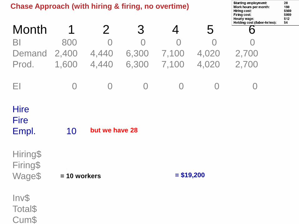
Month 1 2 3 4 5 6 BI 800 0 0 0 0 0
Demand 2,400 4,440 6,300 7,100 4,020 2,700
Prod. 1,600 4,440 6,300 7,100 4,020 2,700
EI 0 0 0 0 0 0
Hire 18 12 5
Fire 18 19 9
Empl. 10 28 40 45 26 17
Hiring$ 9,000 6,000 2,500
Firing$ 14,400 15,200 7,200
Wage$ 19,200 53,760 76,800 86,400 49,920 32,640
Inv$ 0 0 0 0 0 0
Total$ 33,600 62,760 82,800 88,900 65,120 39,840
Cum$ 33,600 96,360 179,160 268,060 333,180 373,020
Chase Approach (with hiring & firing, no overtime)
# workers
needed in
month 1
1600 hr/mo
160 hr/mo
1 worker
= 10 workers =
Under chase production
how much will we produce
in each period??
Month 1 2 3 4 5 6 BI 800 0 0 0 0 0
Demand 2,400 4,440 6,300 7,100 4,020 2,700
Prod. 1,600 4,440 6,300 7,100 4,020 2,700
EI 0 0 0 0 0 0
Hire 18 12 5
Fire 18 19 9
Empl. 10 28 40 45 26 17
Hiring$ 9,000 6,000 2,500
Firing$ 14,400 15,200 7,200
Wage$ 19,200 53,760 76,800 86,400 49,920 32,640
Inv$ 0 0 0 0 0 0
Total$ 33,600 62,760 82,800 88,900 65,120 39,840
Cum$ 33,600 96,360 179,160 268,060 333,180 373,020
Chase Approach (with hiring & firing, no overtime)
but we have 28
= 10 workers x 160 hr x $12
mo hr
= $19,200

Month 1 2 3 4 5 6 BI 800 0 0 0 0 0
Demand 2,400 4,440 6,300 7,100 4,020 2,700
Prod. 1,600 4,440 6,300 7,100 4,020 2,700
EI 0 0 0 0 0 0
Hire 18 12 5
Fire 18 19 9
Empl. 10 28 40 45 26 17
Hiring$ 9,000 6,000 2,500
Firing$ 14,400 15,200 7,200
Wage$ 19,200 53,760 76,800 86,400 49,920 32,640
Inv$ 0 0 0 0 0 0
Total$ 33,600 62,760 82,800 88,900 65,120 39,840
Cum$ 33,600 96,360 179,160 268,060 333,180 373,020
Chase Approach (with hiring & firing, no overtime)
4440 hr/mo
160 hr/mo
1 worker
~ 28 workers = # workers
needed in
month 2

Month 1 2 3 4 5 6 BI 800 0 0 0 0 0
Demand 2,400 4,440 6,300 7,100 4,020 2,700
Prod. 1,600 4,440 6,300 7,100 4,020 2,700
EI 0 0 0 0 0 0
Hire 18 12 5
Fire 18 19 9
Empl. 10 28 40 45 26 17
Hiring$ 9,000 6,000 2,500
Firing$ 14,400 15,200 7,200
Wage$ 19,200 53,760 76,800 86,400 49,920 32,640
Inv$ 0 0 0 0 0 0
Total$ 33,600 62,760 82,800 88,900 65,120 39,840
Cum$ 33,600 96,360 179,160 268,060 333,180 373,020
Chase Approach (with hiring & firing, no overtime)
but we only have 10
= 28 workers x 160 hr x $12
mo hr
= $53,760

Month 1 2 3 4 5 6 BI 800 0 0 0 0 0
Demand 2,400 4,440 6,300 7,100 4,020 2,700
Prod. 1,600 4,440 6,300 7,100 4,020 2,700
EI 0 0 0 0 0 0
Hire 18 12 5
Fire 18 19 9
Empl. 10 28 40 45 26 17
Hiring$ 9,000 6,000 2,500
Firing$ 14,400 15,200 7,200
Wage$ 19,200 53,760 76,800 86,400 49,920 32,640
Inv$ 0 0 0 0 0 0
Total$ 33,600 62,760 82,800 88,900 65,120 39,840
Cum$ 33,600 96,360 179,160 268,060 333,180 373,020
Chase Approach (with hiring & firing, no overtime)
but we only have 28
= 40 workers x 160 hr x $12
mo hr
= $76,800
Again, this process
continues for
each period…
6300 hr/mo
160 hr/mo
1 worker
~ 40 workers = # workers
needed in
month 3

Month 1 2 3 4 5 6 BI 800 0 0 0 0 0
Demand 2,400 4,440 6,300 7,100 4,020 2,700
Prod. 1,600 4,440 6,300 7,100 4,020 2,700
EI 0 0 0 0 0 0
Hire 18 12 5
Fire 18 19 9
Empl. 10 28 40 45 26 17
Hiring$ 9,000 6,000 2,500
Firing$ 14,400 15,200 7,200
Wage$ 19,200 53,760 76,800 86,400 49,920 32,640
Inv$ 0 0 0 0 0 0
Total$ 33,600 62,760 82,800 88,900 65,120 39,840
Cum$ 33,600 96,360 179,160 268,060 333,180 373,020
Chase Approach (with hiring & firing, no overtime)

Three General Strategic Plans
1. Level – constant workforce/production level – fluctuating inventory levels
2. Chase – production and manpower fluctuate
3. Stable Workforce – size of workforce is constant – number of hours worked fluctuates
How to meet changes in demand

Month 1 2 3 4 5 6 BI 800 0 0 0 0 0
Demand 2,400 4,440 6,300 7,100 4,020 2,700
RT Prod. 1,600 4,440 4,480 4,480 4,020 2,700
OT Prod. 1,820 2,620
EI 0 0 0 0 0 0
Empl. 28 28 28 28 28 28
Hiring$
Firing$
RTWage$ 53,760 53,760 53,760 53,760 53,760 53,760
OTWage$ 32,760 47,160
Inv$ 0 0 0 0 0 0
Total$ 53,760 53,760 86,520 100,920 53,760 53,760
Cum$ 53,760 107,520 194,040 294,960 348,720 402,480
Stable Workforce – Variable Hours
Now, instead of just regular production we can have…
OT wage = 1.5 x regular wage

Month 1 2 3 4 5 6 BI 800 0 0 0 0 0
Demand 2,400 4,440 6,300 7,100 4,020 2,700
RT Prod. 1,600 4,440 4,480 4,480 4,020 2,700
OT Prod. 1,820 2,620
EI 0 0 0 0 0 0
Empl. 28 28 28 28 28 28
Hiring$
Firing$
RTWage$ 53,760 53,760 53,760 53,760 53,760 53,760
OTWage$ 32,760 47,160
Inv$ 0 0 0 0 0 0
Total$ 53,760 53,760 86,520 100,920 53,760 53,760
Cum$ 53,760 107,520 194,040 294,960 348,720 402,480
Stable Workforce – Variable Hours
Stable workforce = 28 employees
Regular work hours per month per employee = 160 hr
Maximum regular time production per month = 28 x 160 = 4480
OT wage = 1.5 x regular wage

Month 1 2 3 4 5 6 BI 800 0 0 0 0 0
Demand 2,400 4,440 6,300 7,100 4,020 2,700
RT Prod. 1,600 4,440 4,480 4,480 4,020 2,700
OT Prod. 1,820 2,620
EI 0 0 0 0 0 0
Empl. 28 28 28 28 28 28
Hiring$
Firing$
RTWage$ 19,200 53,280 53,760 53,760 48,240 32,400
OTWage$ 32,760 47,160
Inv$ 0 0 0 0 0 0
Total$ 19,200 53,280 86,520 100,920 48,240 32,400
Cum$ 19,200 72,480 159,000 259,920 308,160 340,560
Stable Workforce – Variable Hours
Again, this process
continues for
each period…
OT wage = 1.5 x regular wage
= 1600 labor-hr x $12/hr
= 1820 labor-hr x ($12/hr x 1.5)

Month 1 2 3 4 5 6 BI 800 0 0 0 0 0
Demand 2,400 4,440 6,300 7,100 4,020 2,700
RT Prod. 1,600 4,440 4,480 4,480 4,020 2,700
OT Prod. 1,820 2,620
EI 0 0 0 0 0 0
Empl. 28 28 28 28 28 28
Hiring$
Firing$
RTWage$ 19,200 53,280 53,760 53,760 48,240 32,400
OTWage$ 32,760 47,160
Inv$ 0 0 0 0 0 0
Total$ 19,200 53,280 86,520 100,920 48,240 32,400
Cum$ 19,200 72,480 159,000 259,920 308,160 340,560
Stable Workforce – Variable Hours OT wage = 1.5 x regular wage

Month 1 2 3 4 5 6 BI 800 0 0 0 0 0
Demand 2,400 4,440 6,300 7,100 4,020 2,700
RT Prod. 1,600 4,440 4,480 4,480 4,020 2,700
OT Prod. 1,820 2,620
EI 0 0 0 0 0 0
Empl. 28 28 28 28 28 28
Hiring$
Firing$
RTWage$ 53,760 53,760 53,760 53,760 53,760 53,760
OTWage$ 32,760 47,160
Inv$ 0 0 0 0 0 0
Total$ 53,760 53,760 86,520 100,920 53,760 53,760
Cum$ 53,760 107,520 194,040 294,960 348,720 402,480
Stable Workforce – Variable Hours (mandatory 40 hours)
28 workers x 160 hr/mo x $12/hr = $53,760 = Regular
Time pay Now we need to pay
each worker for a 40 hour work week
(regardless of time worked)
plus any overtime

Month 1 2 3 4 5 6 BI 800 0 0 0 0 0
Demand 2,400 4,440 6,300 7,100 4,020 2,700
RT Prod. 1,600 4,440 4,480 4,480 4,020 2,700
OT Prod. 1,820 2,620
EI 0 0 0 0 0 0
Empl. 28 28 28 28 28 28
Hiring$
Firing$
RTWage$ 53,760 53,760 53,760 53,760 53,760 53,760
OTWage$ 32,760 47,160
Inv$ 0 0 0 0 0 0
Total$ 53,760 53,760 86,520 100,920 53,760 53,760
Cum$ 53,760 107,520 194,040 294,960 348,720 402,480
Stable Workforce – Variable Hours (mandatory 40 hours)

Summary
• Aggregate Planning Definition
• Options for Influencing Demand / Supply
• Iterative Nature of Planning
• Cost Factors
• Sales an Operations Planning in Service Environments
• Production Strategies