Modified arctan-gravity model mimicking a cosmological constant

S. I. KruglovDepartment of Chemical and Physical Sciences, University of Toronto, 3359 Mississauga Road North,

Mississauga, Ontario L5L 1C6, Canada(Received 24 October 2013; revised manuscript received 6 January 2014; published 4 March 2014)

A novel theory of FðRÞ gravity with the Lagrangian density L ¼ ½R − ðb=βÞ arctan ðβRÞ�=ð2κ2Þ isanalyzed. Constant curvature solutions of the model are found, and the potential of the scalar field and themass of a scalar degree of freedom in Einstein’s frame are derived. The cosmological parameters of themodel are calculated, which are in agreement with the PLANCK data. Critical points for the de Sitter phaseand the matter dominated epoch of autonomous equations are obtained and studied.

DOI: 10.1103/PhysRevD.89.064004 PACS numbers: 95.36.+x, 04.50.Kd, 98.80.Es

I. INTRODUCTION

Inflationary cosmology, introduced by Guth [1],remains the main point of view in modern cosmology.It can solve the problem of the initial conditions toexplain the formation of galaxies and irregularities inthe microwave background. Therefore, it is important tosuggest the model that describes correctly the inflationaryepoch in accordance with the experimental data. Theevolution of the Universe can be characterized by thecosmological parameters that were measured by WMAPand recent PLANCK experiments, allowing us to selectthe viable model from the many models suggested. TheΛ-Cold Dark Matter (ΛCDM) model introducing thecosmological constant Λ [2] remains a good candidatefor a description of dark energy (DE) and all observationaldata of the accelerated expansion. But this model suffersdifficulty with the explanation of the smallness of Λcompared with the vacuum energy of elementary particles.To describe the accelerated Universe at the present time,the single-field model with dynamical dark energy may beused [3]. Here we pay attention to FðRÞ-gravity theoriesand the modification of the general relativity (GR),replacing the Ricci scalar in Einstein-Hilbert action bythe function FðRÞ [4–7]. FðRÞ-gravity models contain asingle extra degree of freedom (a scalar) and can bereformulated in a scalar-tensor form. Such purely gravi-tational models describe the inflation, modify gravitationalphysics, and are an alternative to the ΛCDM model. Thefirst successful models of FðRÞ gravity were given in[8–11]. Some models of FðRÞ-gravity theories were con-sidered in [12–21], and in many other publications. Therequirement is that the scalar field is not a tachyon and aghost leads to the condition F00ðRÞ > 0 (primes meanderivatives with respect to an argument). At the same timethe inequality F0ðRÞ > 0 guarantees that a graviton is not aghost [11]. The FðRÞ gravity is a phenomenologicaleffective model that describes geometrical DE. If theFðRÞ-gravity model really describes the evolution of ourUniverse, the present and primordial DE, it should followfrom the fundamental theory like string or M theory.

In this paper we consider the choice of the functioncorresponding to Fð0Þ¼0, FðRÞ → R − 2Λeff at R ≫ Λeff ,where Λeff is the effective cosmological constant. The Λeffis not zero in curved space-time but is zero in the flat space-time. Such a model mimics the cosmological constant atlarge R due to geometry, and Λeff is not connected withquantum vacuum energy. Such a class of models wasalready considered in [9–11]. Here we suggest anotherFðRÞ-gravity model that passes cosmological tests.The paper is organized as follows. In Sec. II we

formulate the model showing the classical and quantumstabilities. The constant curvature solutions of equations ofmotion are obtained and the de Sitter phases are considered.After performing the conformal transformation of themetric, we obtain the scalar-tensor form of the model inEinstein’s frame in Sec. III. The potential of the scalar fieldand the mass of a scalaron are derived, and the plots of thefunctions ϕðβRÞ, VðβRÞ, VðϕÞ, and m2

ϕðβRÞ for differentvalues of the parameter b are given. In Sec. IV thecosmological slow-roll parameters of the model are evalu-ated, and the plots of ϵðβRÞ, ηðβRÞ, and nsðβRÞ arepresented. In Sec. V critical points of autonomous equa-tions are investigated, showing that the matter dominatedepoch is viable. The function mðrÞ characterizing thedeviation from the ΛCDM model is calculated and theplot is given. The effective gravitational constant related tothe evolution of matter density perturbations is studied.Section VI is devoted to the conclusion.The Minkowski metric ημν ¼ diagð−1; 1; 1; 1Þ is used,

and c ¼ ℏ ¼ 1 is assumed throughout the paper.

II. THE MODEL

Let us consider the gravitation theory where we replacethe Ricci scalar R in the Einstein-Hilbert action by thefunction

FðRÞ ¼ Rþ fðRÞ; fðRÞ ¼ −bβarctan ðβRÞ; (1)

and we imply that β > 0, R > 0. The constant β has thedimension of ðlengthÞ2 and b is the dimensionless constant.

PHYSICAL REVIEW D 89, 064004 (2014)

1550-7998=2014=89(6)=064004(8) 064004-1 © 2014 American Physical Society

The function FðRÞ satisfies the conditions Fð0Þ ¼ 0,limR→∞fðRÞ ¼ const, which are necessary to mimic thephenomenology of the ΛCDM model in the high-redshiftregime. Thus, the action in the Jordan frame becomes

S ¼Z

d4xffiffiffiffiffiffi−gp

L ¼Z

d4xffiffiffiffiffiffi−gp �

1

2κ2FðRÞ þ Lm

�; (2)

where κ ¼ M−1Pl ,MPl is the reduced Planck mass, and Lm is

the matter Lagrangian density. From Eq. (1) one obtains

F0ðRÞ ¼ 1 − b1þ ðβRÞ2 ; F00ðRÞ ¼ 2bβ2R

ð1þ ðβRÞ2Þ2 ;(3)

where primes denote the derivatives on argument. Thefunction FðRÞ obeys the condition F00ðRÞ > 0 at b > 0,which ensures the classical stability of the solution at highcurvature. It follows from Eq. (3) that the condition ofquantum stability F0ðRÞ > 0 leads to

1þ ðβRÞ2 > b: (4)

Thus, 0 < b < 1.

A. Constant curvature solutions

Let us consider constant curvature solutions to equationsof motion that follow from the action (2) without matter.Such an equation of motion is given by [22]

2FðRÞ − RF0ðRÞ ¼ 0: (5)

It should be noted that Eq. (5) corresponds to the extremumof the effective potential of the scalar degree of freedom (inEinstein’s frame). With the help of Eqs. (1) and (5) weobtain

b

�2 arctanðβRÞ − βR

1þ ðβRÞ2�

¼ βR: (6)

Equation (6) possesses the solution R0 ¼ 0 correspondingto the Minkowski space-time. Nontrivial solutions of thetranscendental equation (6) for the model with b ¼ 0.99 aregiven by

βR1 ≈ 0.1791 ðκϕ1 ≈ 3.919Þ;βR2 ≈ 1.4582 ðκϕ2 ≈ 0.466Þ;

and for b ¼ 0.999 are

βR1 ≈ 0.05495 ðκϕ1 ≈ 6.760Þ;βR2 ≈ 1.5094 ðκϕ2 ≈ 0.445Þ:

It should be noted that for b ≤ 0.9 Eq. (6) has only trivialsolution R0 ¼ 0, which goes with flat space-time.

Nontrivial constant curvature solutions R1 and R2 leadto the Schwarzschild—de Sitter space and correspond toinflation. If the condition F0ðRÞ=F00ðRÞ > R is satisfied,then it can describe primordial and present dark energy,which are future stable [23]. From Eq. (3), one obtains

F0ðRÞF00ðRÞ ¼

½1þ ðβRÞ2�½1þ ðβRÞ2 − b�2bβ2R

: (7)

It can be verified that the constant curvature solutions R1

are unstable because F0ðR1Þ=F00ðR1Þ < R1 and correspondto the maximum of the potential for scalaron (a scalardegree of freedom) and solutions R2 are stable asF0ðR2Þ=F00ðR2Þ > R2 and correspond to the minimum ofthe potential for scalaron. The spherically symmetric metricof the Schwarzschild form is given by

ds2 ¼ −BðrÞdt2 þ dr2

BðrÞ þ r2ðdθ2 þ sin2θdϕ2Þ: (8)

FðRÞ-gravity theories with the constant Ricci scalar R > 0have Schwarzschild—de Sitter solutions with the functionBðrÞ,

BðrÞ ¼ 1 − 2 MGr

− R12

r2; (9)

possessing the classical stability of Schwarzschild blackholes; G is the Newton constant and M is the mass of theblack hole. Einstein’s equation solutions with the cosmo-logical constant Λ have the function of the form (9) withR ¼ 4Λ. Thus, the model under consideration possesses thedynamical cosmological constants. Therefore, for the spacewithout any matter, our model mimics DE (the cosmo-logical constant).In the homogeneous, isotropic, and spatially flat

Friedmann-Robertson-Walker cosmology the Ricci scalarR is given by R ¼ 12H2 þ 6H

:, whereH ¼ a

: ðtÞ=aðtÞ is theHubble parameter. For the case when the Hubble parameteris constant, H0 ¼

ffiffiffiffiffiffiffiffiffiffiffiR=12

p(R is the constant curvature

solution), we have a de Sitter phase. Then a scale factorbecomes aðtÞ ¼ a0 expðH0tÞ (a0 is a scale factor at acosmic time t ¼ 0), and this solution describes the eternalinflation phase.

III. THE SCALAR-TENSOR FORM

In the Einstein frame, corresponding to the scalar-tensortheory of gravity, we have conformally transformedmetric [24]

~gμν ¼ F0ðRÞgμν ¼1 − bþ ðβRÞ21þ ðβRÞ2 gμν: (10)

In this frame action (2), at Lm ¼ 0, is given by

S. I. KRUGLOV PHYSICAL REVIEW D 89, 064004 (2014)

064004-2

S ¼Z

d4xffiffiffiffiffiffi−gp �

1

2κ2~R − 1

2~gμν∇μϕ∇νϕ − VðϕÞ

�; (11)

where ∇μ is the covariant derivative, and ~R is calculatedwith the help of new metric (10). The scalar field ϕ and thepotential VðϕÞ read

ϕ ¼ −ffiffiffi3

plnF0ðRÞffiffiffi2

pκ

¼ffiffiffi3

pffiffiffi2

pκln

�1þ ðβRÞ2

1 − bþ ðβRÞ2�; (12)

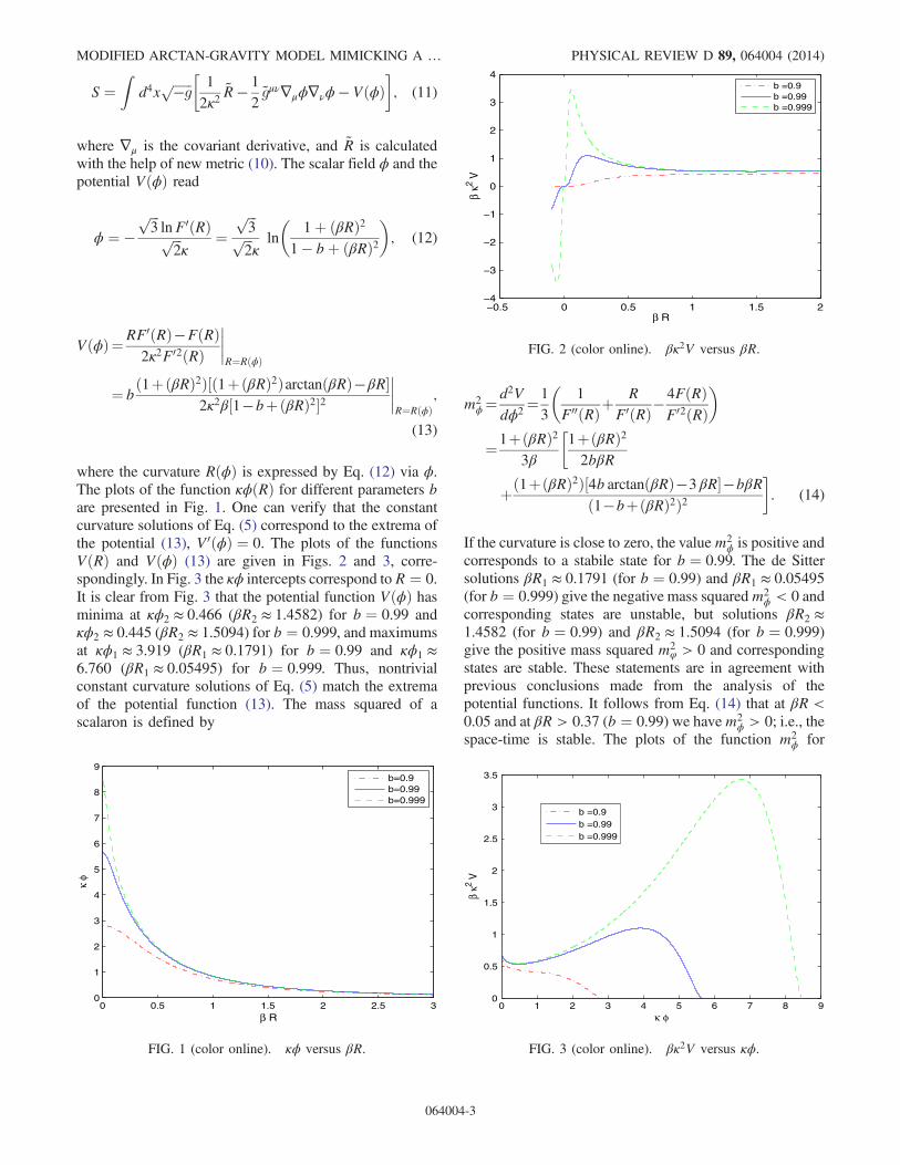
VðϕÞ¼RF0ðRÞ−FðRÞ2κ2F02ðRÞ

����R¼RðϕÞ

¼ bð1þðβRÞ2Þ½ð1þðβRÞ2ÞarctanðβRÞ−βR�

2κ2β½1−bþðβRÞ2�2����R¼RðϕÞ

;

(13)

where the curvature RðϕÞ is expressed by Eq. (12) via ϕ.The plots of the function κϕðRÞ for different parameters bare presented in Fig. 1. One can verify that the constantcurvature solutions of Eq. (5) correspond to the extrema ofthe potential (13), V 0ðϕÞ ¼ 0. The plots of the functionsVðRÞ and VðϕÞ (13) are given in Figs. 2 and 3, corre-spondingly. In Fig. 3 the κϕ intercepts correspond to R ¼ 0.It is clear from Fig. 3 that the potential function VðϕÞ hasminima at κϕ2 ≈ 0.466 (βR2 ≈ 1.4582) for b ¼ 0.99 andκϕ2 ≈ 0.445 (βR2 ≈ 1.5094) for b ¼ 0.999, and maximumsat κϕ1 ≈ 3.919 (βR1 ≈ 0.1791) for b ¼ 0.99 and κϕ1 ≈6.760 (βR1 ≈ 0.05495) for b ¼ 0.999. Thus, nontrivialconstant curvature solutions of Eq. (5) match the extremaof the potential function (13). The mass squared of ascalaron is defined by

m2ϕ¼

d2Vdϕ2

¼1

3

�1

F00ðRÞþR

F0ðRÞ−4FðRÞF02ðRÞ

�

¼1þðβRÞ23β

�1þðβRÞ22bβR

þð1þðβRÞ2Þ½4b arctanðβRÞ−3 βR�−bβRð1−bþðβRÞ2Þ2

�: (14)

If the curvature is close to zero, the valuem2ϕ is positive and

corresponds to a stabile state for b ¼ 0.99. The de Sittersolutions βR1 ≈ 0.1791 (for b ¼ 0.99) and βR1 ≈ 0.05495(for b ¼ 0.999) give the negative mass squaredm2

ϕ < 0 andcorresponding states are unstable, but solutions βR2 ≈1.4582 (for b ¼ 0.99) and βR2 ≈ 1.5094 (for b ¼ 0.999)give the positive mass squared m2

φ > 0 and correspondingstates are stable. These statements are in agreement withprevious conclusions made from the analysis of thepotential functions. It follows from Eq. (14) that at βR <0.05 and at βR > 0.37 (b ¼ 0.99) we havem2

ϕ > 0; i.e., thespace-time is stable. The plots of the function m2

ϕ for

0 0.5 1 1.5 2 2.5 30

1

2

3

4

5

6

7

8

9

β R

κφ

b=0.9b=0.99b=0.999

FIG. 1 (color online). κϕ versus βR.

−0.5 0 0.5 1 1.5 2−4

−3

−2

−1

0

1

2

3

4

β R

βκ2 V

b =0.9b =0.99b =0.999

FIG. 2 (color online). βκ2V versus βR.

0 1 2 3 4 5 6 7 8 90

0.5

1

1.5

2

2.5

3

3.5

κ φ

βκ2 V

b =0.9b =0.99b =0.999

FIG. 3 (color online). βκ2V versus κϕ.

MODIFIED ARCTAN-GRAVITY MODEL MIMICKING A … PHYSICAL REVIEW D 89, 064004 (2014)

064004-3

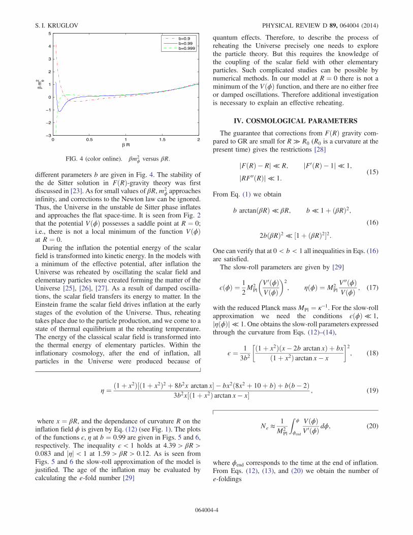
different parameters b are given in Fig. 4. The stability ofthe de Sitter solution in FðRÞ-gravity theory was firstdiscussed in [23]. As for small values of βR,m2

ϕ approachesinfinity, and corrections to the Newton law can be ignored.Thus, the Universe in the unstable de Sitter phase inflatesand approaches the flat space-time. It is seen from Fig. 2that the potential VðϕÞ possesses a saddle point at R ¼ 0;i.e., there is not a local minimum of the function VðϕÞat R ¼ 0.During the inflation the potential energy of the scalar

field is transformed into kinetic energy. In the models witha minimum of the effective potential, after inflation theUniverse was reheated by oscillating the scalar field andelementary particles were created forming the matter of theUniverse [25], [26], [27]. As a result of damped oscilla-tions, the scalar field transfers its energy to matter. In theEinstein frame the scalar field drives inflation at the earlystages of the evolution of the Universe. Thus, reheatingtakes place due to the particle production, and we come to astate of thermal equilibrium at the reheating temperature.The energy of the classical scalar field is transformed intothe thermal energy of elementary particles. Within theinflationary cosmology, after the end of inflation, allparticles in the Universe were produced because of

quantum effects. Therefore, to describe the process ofreheating the Universe precisely one needs to explorethe particle theory. But this requires the knowledge ofthe coupling of the scalar field with other elementaryparticles. Such complicated studies can be possible bynumerical methods. In our model at R ¼ 0 there is not aminimum of the VðϕÞ function, and there are no either freeor damped oscillations. Therefore additional investigationis necessary to explain an effective reheating.

IV. COSMOLOGICAL PARAMETERS

The guarantee that corrections from FðRÞ gravity com-pared to GR are small for R ≫ R0 (R0 is a curvature at thepresent time) gives the restrictions [28]

∣FðRÞ − R∣ ≪ R; ∣F0ðRÞ − 1∣ ≪ 1;

∣RF00ðRÞ∣ ≪ 1:(15)

From Eq. (1) we obtain

b arctanðβRÞ ≪ βR; b ≪ 1þ ðβRÞ2;(16)

2bðβRÞ2 ≪ ½1þ ðβRÞ2�2:One can verify that at 0 < b < 1 all inequalities in Eqs. (16)are satisfied.The slow-roll parameters are given by [29]

ϵðϕÞ ¼ 1

2M2

Pl

�V 0ðϕÞVðϕÞ

�2

; ηðϕÞ ¼ M2PlV 00ðϕÞVðϕÞ ; (17)

with the reduced Planck mass MPl ¼ κ−1. For the slow-rollapproximation we need the conditions ϵðϕÞ ≪ 1,∣ηðϕÞ∣ ≪ 1. One obtains the slow-roll parameters expressedthrough the curvature from Eqs. (12)–(14),

ϵ ¼ 1

3b2

�ð1þ x2Þðx − 2b arctan xÞ þ bxð1þ x2Þ arctan x − x

�2

; (18)

η ¼ ð1þ x2Þ½ð1þ x2Þ2 þ 8b2x arctan x� − bx2ð8x2 þ 10þ bÞ þ bðb − 2Þ3b2x½ð1þ x2Þ arctan x − x� ; (19)

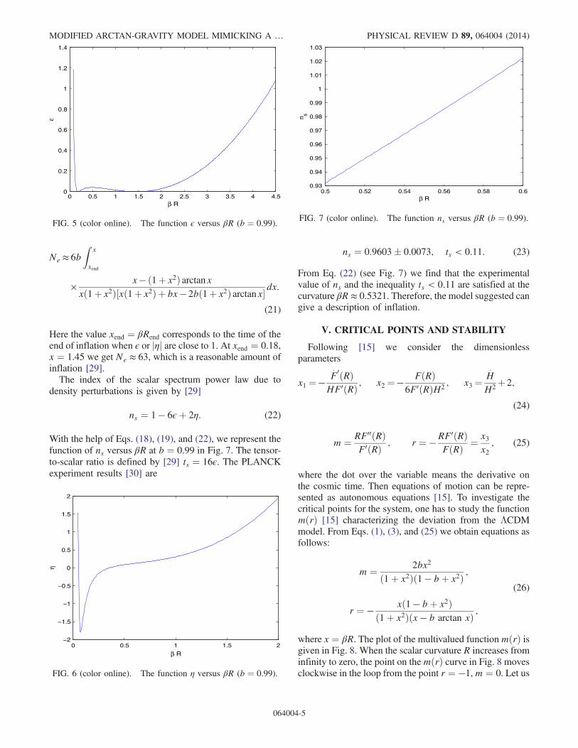
where x ¼ βR, and the dependance of curvature R on theinflation field ϕ is given by Eq. (12) (see Fig. 1). The plotsof the functions ϵ, η at b ¼ 0.99 are given in Figs. 5 and 6,respectively. The inequality ϵ < 1 holds at 4.39 > βR >0.083 and jηj < 1 at 1.59 > βR > 0.12. As is seen fromFigs. 5 and 6 the slow-roll approximation of the model isjustified. The age of the inflation may be evaluated bycalculating the e-fold number [29]

Ne ≈1

M2Pl

Zϕ

ϕend

VðϕÞV 0ðϕÞ dϕ; (20)

where ϕend corresponds to the time at the end of inflation.From Eqs. (12), (13), and (20) we obtain the number ofe-foldings

0 0.5 1 1.5 2−3

−2

−1

0

1

2

3

4

5

β R

β m

2 φb=0.9b=0.99b=0.999

FIG. 4 (color online). βm2ϕ versus βR.

S. I. KRUGLOV PHYSICAL REVIEW D 89, 064004 (2014)

064004-4

Ne ≈ 6bZ

x

xend

×x− ð1þ x2Þ arctanx

xð1þ x2Þ½xð1þ x2Þ þ bx− 2bð1þ x2Þ arctanx�dx:

(21)

Here the value xend ¼ βRend corresponds to the time of theend of inflation when ϵ or jηj are close to 1. At xend ¼ 0.18,x ¼ 1.45 we get Ne ≈ 63, which is a reasonable amount ofinflation [29].The index of the scalar spectrum power law due to

density perturbations is given by [29]

ns ¼ 1 − 6ϵþ 2η: (22)

With the help of Eqs. (18), (19), and (22), we represent thefunction of ns versus βR at b ¼ 0.99 in Fig. 7. The tensor-to-scalar ratio is defined by [29] ts ¼ 16ϵ. The PLANCKexperiment results [30] are

ns ¼ 0.9603� 0.0073; ts < 0.11: (23)

From Eq. (22) (see Fig. 7) we find that the experimentalvalue of ns and the inequality ts < 0.11 are satisfied at thecurvature βR ≈ 0.5321. Therefore, the model suggested cangive a description of inflation.

V. CRITICAL POINTS AND STABILITY

Following [15] we consider the dimensionlessparameters

x1 ¼− F: 0ðRÞ

HF0ðRÞ ; x2 ¼− FðRÞ6F0ðRÞH2

; x3 ¼H:

H2þ 2;

(24)

m ¼ RF00ðRÞF0ðRÞ ; r ¼ −RF0ðRÞ

FðRÞ ¼ x3x2

; (25)

where the dot over the variable means the derivative onthe cosmic time. Then equations of motion can be repre-sented as autonomous equations [15]. To investigate thecritical points for the system, one has to study the functionmðrÞ [15] characterizing the deviation from the ΛCDMmodel. From Eqs. (1), (3), and (25) we obtain equations asfollows:

m ¼ 2bx2

ð1þ x2Þð1 − bþ x2Þ ;(26)

r ¼ − xð1 − bþ x2Þð1þ x2Þðx − b arctan xÞ ;

where x ¼ βR. The plot of the multivalued functionmðrÞ isgiven in Fig. 8. When the scalar curvature R increases frominfinity to zero, the point on themðrÞ curve in Fig. 8 movesclockwise in the loop from the point r ¼ −1,m ¼ 0. Let us

0.5 0.52 0.54 0.56 0.58 0.60.93

0.94

0.95

0.96

0.97

0.98

0.99

1

1.01

1.02

1.03

β R

n s

FIG. 7 (color online). The function ns versus βR (b ¼ 0.99).

0 0.5 1 1.5 2−2

−1.5

−1

−0.5

0

0.5

1

1.5

2

β R

η

FIG. 6 (color online). The function η versus βR (b ¼ 0.99).

0 0.5 1 1.5 2 2.5 3 3.5 4 4.50

0.2

0.4

0.6

0.8

1

1.2

1.4

β R

ε

FIG. 5 (color online). The function ϵ versus βR (b ¼ 0.99).

MODIFIED ARCTAN-GRAVITY MODEL MIMICKING A … PHYSICAL REVIEW D 89, 064004 (2014)

064004-5

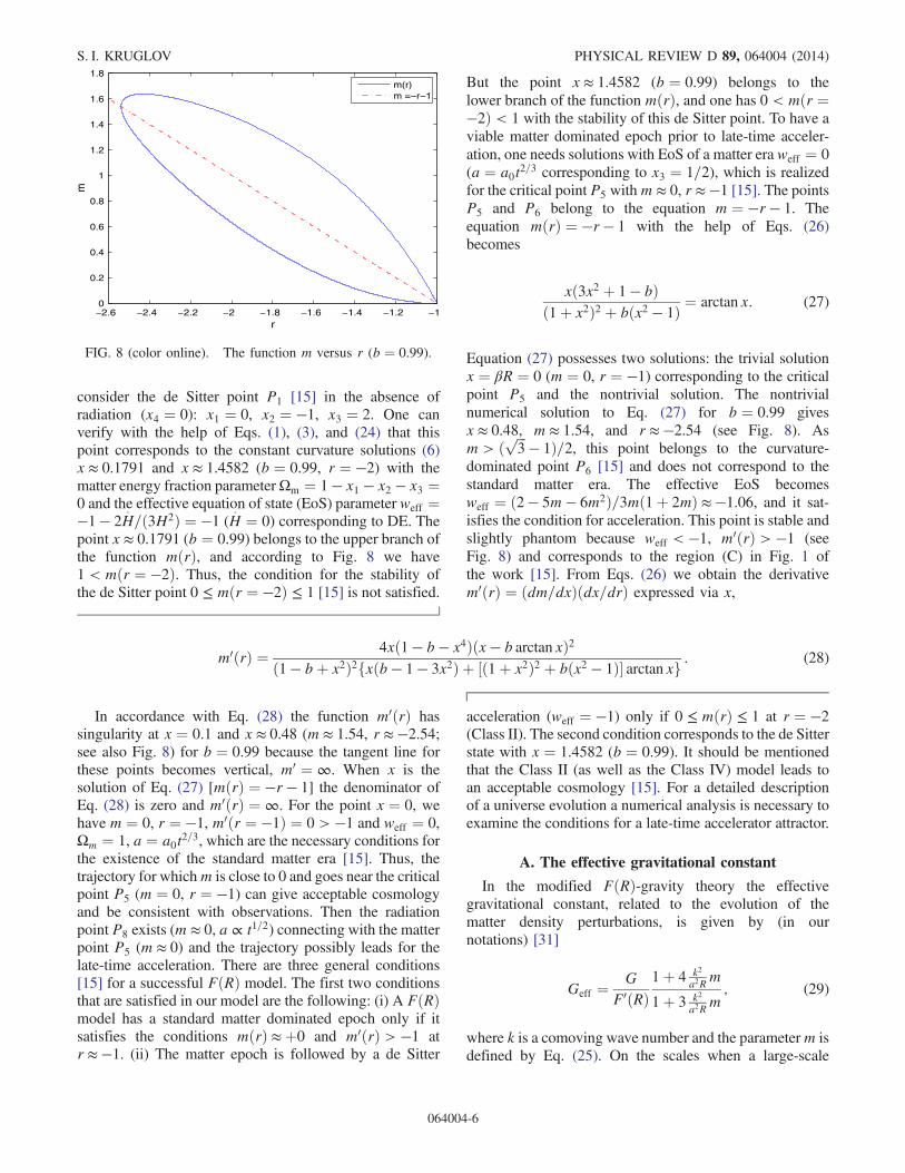
consider the de Sitter point P1 [15] in the absence ofradiation (x4 ¼ 0): x1 ¼ 0, x2 ¼ −1, x3 ¼ 2. One canverify with the help of Eqs. (1), (3), and (24) that thispoint corresponds to the constant curvature solutions (6)x ≈ 0.1791 and x ≈ 1.4582 (b ¼ 0.99, r ¼ −2) with thematter energy fraction parameterΩm ¼ 1 − x1 − x2 − x3 ¼0 and the effective equation of state (EoS) parameter weff ¼−1 − 2H

:=ð3H2Þ ¼ −1 (H

: ¼ 0) corresponding to DE. Thepoint x ≈ 0.1791 (b ¼ 0.99) belongs to the upper branch ofthe function mðrÞ, and according to Fig. 8 we have1 < mðr ¼ −2Þ. Thus, the condition for the stability ofthe de Sitter point 0 ≤ mðr ¼ −2Þ ≤ 1 [15] is not satisfied.

But the point x ≈ 1.4582 (b ¼ 0.99) belongs to thelower branch of the function mðrÞ, and one has 0 < mðr ¼−2Þ < 1 with the stability of this de Sitter point. To have aviable matter dominated epoch prior to late-time acceler-ation, one needs solutions with EoS of a matter era weff ¼ 0(a ¼ a0t2=3 corresponding to x3 ¼ 1=2), which is realizedfor the critical point P5 withm ≈ 0, r ≈ −1 [15]. The pointsP5 and P6 belong to the equation m ¼ −r − 1. Theequation mðrÞ ¼ −r − 1 with the help of Eqs. (26)becomes

xð3x2 þ 1 − bÞð1þ x2Þ2 þ bðx2 − 1Þ ¼ arctan x: (27)

Equation (27) possesses two solutions: the trivial solutionx ¼ βR ¼ 0 (m ¼ 0, r ¼ −1) corresponding to the criticalpoint P5 and the nontrivial solution. The nontrivialnumerical solution to Eq. (27) for b ¼ 0.99 givesx ≈ 0.48, m ≈ 1.54, and r ≈ −2.54 (see Fig. 8). Asm > ð ffiffiffi

3p − 1Þ=2, this point belongs to the curvature-

dominated point P6 [15] and does not correspond to thestandard matter era. The effective EoS becomesweff ¼ ð2 − 5m − 6m2Þ=3mð1þ 2mÞ ≈ −1.06, and it sat-isfies the condition for acceleration. This point is stable andslightly phantom because weff < −1, m0ðrÞ > −1 (seeFig. 8) and corresponds to the region (C) in Fig. 1 ofthe work [15]. From Eqs. (26) we obtain the derivativem0ðrÞ ¼ ðdm=dxÞðdx=drÞ expressed via x,

m0ðrÞ ¼ 4xð1 − b − x4Þðx − b arctan xÞ2ð1 − bþ x2Þ2fxðb − 1 − 3x2Þ þ ½ð1þ x2Þ2 þ bðx2 − 1Þ� arctan xg : (28)

In accordance with Eq. (28) the function m0ðrÞ hassingularity at x ¼ 0.1 and x ≈ 0.48 (m ≈ 1.54, r ≈ −2.54;see also Fig. 8) for b ¼ 0.99 because the tangent line forthese points becomes vertical, m0 ¼ ∞. When x is thesolution of Eq. (27) [mðrÞ ¼ −r − 1] the denominator ofEq. (28) is zero and m0ðrÞ ¼ ∞. For the point x ¼ 0, wehave m ¼ 0, r ¼ −1, m0ðr ¼ −1Þ ¼ 0 > −1 and weff ¼ 0,Ωm ¼ 1, a ¼ a0t2=3, which are the necessary conditions forthe existence of the standard matter era [15]. Thus, thetrajectory for whichm is close to 0 and goes near the criticalpoint P5 (m ¼ 0, r ¼ −1) can give acceptable cosmologyand be consistent with observations. Then the radiationpoint P8 exists (m ≈ 0, a ∝ t1=2) connecting with the matterpoint P5 (m ≈ 0) and the trajectory possibly leads for thelate-time acceleration. There are three general conditions[15] for a successful FðRÞ model. The first two conditionsthat are satisfied in our model are the following: (i) A FðRÞmodel has a standard matter dominated epoch only if itsatisfies the conditions mðrÞ ≈þ0 and m0ðrÞ > −1 atr ≈ −1. (ii) The matter epoch is followed by a de Sitter

acceleration (weff ¼ −1) only if 0 ≤ mðrÞ ≤ 1 at r ¼ −2(Class II). The second condition corresponds to the de Sitterstate with x ¼ 1.4582 (b ¼ 0.99). It should be mentionedthat the Class II (as well as the Class IV) model leads toan acceptable cosmology [15]. For a detailed descriptionof a universe evolution a numerical analysis is necessary toexamine the conditions for a late-time accelerator attractor.

A. The effective gravitational constant

In the modified FðRÞ-gravity theory the effectivegravitational constant, related to the evolution of thematter density perturbations, is given by (in ournotations) [31]

Geff ¼G

F0ðRÞ1þ 4 k2

a2Rm

1þ 3 k2

a2Rm; (29)

where k is a comoving wave number and the parameterm isdefined by Eq. (25). On the scales when a large-scale

−2.6 −2.4 −2.2 −2 −1.8 −1.6 −1.4 −1.2 −10

0.2

0.4

0.6

0.8

1

1.2

1.4

1.6

1.8

r

mm(r)m =−r−1

FIG. 8 (color online). The function m versus r (b ¼ 0.99).

S. I. KRUGLOV PHYSICAL REVIEW D 89, 064004 (2014)

064004-6

structure is formed, the condition k2m=ða2RÞ ≪ 1 isrealized and Eq. (29) becomes [31]

Geff ¼G

F0ðRÞ�1þ k2m

a2R

�: (30)

In this case the second term in brackets of Eq. (30) is smallas compared with the unit. This condition is satisfied fortrajectories that are close to the critical point P5 becausem ≈ 0. Then the matter density perturbation δm ∝ t2=3, thegravitational potential Φ=const [31], and we come to thestandard result. It should be mentioned that at the presentepoch the local gravity constraint requires the equal-ity k2m=ða2RÞ ≪ 1.The entropy S in FðRÞ-gravity models is given by [32]

S ¼ F0ðRÞA=ð4GÞ, which is the generalization of theBekenstein-Hawking formula, where A is the area of thehorizon. One can obtain the standard formula forthe entropy introducing the effective gravitational couplingGeff ¼ G=F0ðRÞ ¼ G½1þ ðβRÞ2�=½1 − bþ ðβRÞ2�, whichis in accordance with Eq. (30) at k2m=ða2RÞ ≪ 1.

VI. CONCLUSION

The model of FðRÞ gravity under considerationmimics a cosmological constant and admits two de Sittersolutions (P1 points) for r ¼ −2 with βR1 ≈ 0.1791

(m > 1, b ¼ 0.99), which is an unstable state, and withβR2 ≈ 1.4582 (0 < m < 1, b ¼ 0.99), which is the stablestate. Thus, in the model of gravity suggested the cosmicacceleration arises. There are P5, P6 points that are thesolutions of the equation mðrÞ ¼ −r − 1. The critical pointwith r ≈ −2.54, m ≈ 1.54 (βR ≈ 0.48) does not give thestandard matter era. The second critical P5 point corre-sponds to the standard matter era as m ¼ 0, r ¼ −1,m0ðrÞ > −1, and a ¼ a0t2=3. The model suggested belongsto Class II [15]: the mðrÞ curve connects the vicinity of thepoint ðr;mÞ ¼ ð−1; 0Þ to the point P1 (βR2 ≈ 1.4582)located at r ¼ −2 (0 < m < 1). Thus, it was shown thatcritical points P1 and P5, in the classification of autono-mous equations [15], are realized in the model underconsideration and the inflation in this version of FðRÞgravity is possible. As a result, the model can be obser-vationally acceptable. GR may be an approximation thatdescribes the Universe at the intermediate cosmic time. IfβR → ∞, action (2) approaches the Einstein-Hilbert actionwith the cosmological constant. It was shown that the slow-roll approximation holds and the cosmological parameterscalculated are in agreement with the observed CMB data bythe WMAP and PLANCK experiments. To explain all thecosmological periods, from inflation to current acceleratedexpansion, and to check the viability of the model, oneneeds to solve and analyze the autonomous equations [15].We leave such investigation for further study.

[1] A. H. Guth, Phys. Rev. D 23, 347 (1981).[2] J. A. Frieman, M. S. Turner, and D. Huterer, Annu. Rev.

Astron. Astrophys. 46, 385 (2008).[3] A. D. Linde, Particle Physics and Inflationary Cosmology

(Harwood Academic Publishers, Chur, Switzerland, 1992).[4] R. R. Caldwell and M. Kamionkowski, Annu. Rev. Nucl.

Part. Sci. 59, 397 (2009).[5] T. P. Sotiriou and V. Faraoni, Rev. Mod. Phys. 82, 451

(2010).[6] S. Capozziello and V. Faraoni, Beyond Einstein Gravity: A

Survey of Gravitational Theories for Cosmology andAstrophysics (Springer Science+Business Media B.V.,New York, 2011).

[7] S. Nojiri and S. D. Odintsov, Phys. Rep. 505, 59 (2011).[8] A. A. Starobinsky, Phys. Lett. 91B, 99 (1980).[9] W. Hu and I. Sawicki, Phys. Rev. D 76, 064004 (2007).

[10] S. A. Appleby and R. A. Battye, Phys. Lett. B 654, 7 (2007).[11] A. A. Starobinsky, JETP Lett. 86, 157 (2007).[12] S. Deser and G.W. Gibbons, Classical Quantum Gravity 15,

L35 (1998).[13] S. Nojiri and S. D. Odintsov, Phys. Rev. D 68, 123512

(2003).[14] S. M. Carroll, V. Duvvuri, M. Trodden, and M. S. Turner,

Phys. Rev. D 70, 043528 (2004).

[15] L. Amendola, R. Gannouji, D. Polarski, and S. Tsujikawa,Phys. Rev. D 75, 083504 (2007).

[16] G. Cognola, E. Elizalde, S. Nojiri, S. D. Odintsov,L. Sebastiani, and S. Zerbini, Phys. Rev. D 77, 046009(2008).

[17] E. V. Linder, Phys. Rev. D 80, 123528 (2009).[18] M. Bañados and P. G. Ferreira, Phys. Rev. Lett. 105, 011101

(2010).[19] P. Pani, V. Cardoso, and T. Delsate, Phys. Rev. Lett. 107,

031101 (2011).[20] S. I. Kruglov, Int. J. Theor. Phys. 52, 2477 (2013).[21] S. I. Kruglov, Int. J. Mod. Phys. A 28, 1350119 (2013).[22] J. D. Barrow and A. C. Ottewill, J. Phys. A 16, 2757

(1983).[23] V. Müller, H.-J. Schmidt, and A. A. Starobinsky, Phys. Lett.

B 202, 198 (1988).[24] G. Magnano and L. M. Sokolowski, Phys. Rev. D 50, 5039

(1994).[25] L. Kofman, A. D. Linde, and A. A. Starobinsky, Phys. Rev.

D 56, 3258 (1997).[26] H. Motohashi and A. Nishizawa, Phys. Rev. D 86, 083514

(2012).[27] E. V. Arbuzova, A. D. Dolgov, and L. Reverberi, J. Cosmol.

Astropart. Phys. 02 (2012) 049.

MODIFIED ARCTAN-GRAVITY MODEL MIMICKING A … PHYSICAL REVIEW D 89, 064004 (2014)

064004-7

[28] S. A. Appleby, R. A. Battye, and A. A. Starobinsky,J. Cosmol. Astropart. Phys. 06 (2010) 005.

[29] A. R. Liddle and D. H. Lyth, Cosmological Inflation andLarge-scale Structure (Cambridge University Press,Cambridge, UK, 2000).

[30] P. Ade et al. (Planck Collaboration), arXiv:1303.5083;(Planck Collaboration), arXiv:1303.5082; (PlanckCollaboration), arXiv:1303.5076.

[31] S. Tsujikawa, Phys. Rev. D 76, 023514 (2007).[32] M. Akbar and R.-G. Cai, Phys. Lett. B 635, 7 (2006).

S. I. KRUGLOV PHYSICAL REVIEW D 89, 064004 (2014)

064004-8