Modelling HIV: How complicated do we want to make this? · Exponential rise give R 0 = β /µ =...
32
Modelling HIV: How complicated do we want to make this? Brian Williams South African Centre for Epidemiological Modelling and Analysis
Transcript of Modelling HIV: How complicated do we want to make this? · Exponential rise give R 0 = β /µ =...
Modelling HIV: How complicated do we
want to make this?
Brian Williams
South African Centre for Epidemiological Modelling and Analysis

Working with proportions, susceptible people are infected at a per capita rate β ; Infected people die at a per capita rate µ.
The basic SI model S
βSI I
µI
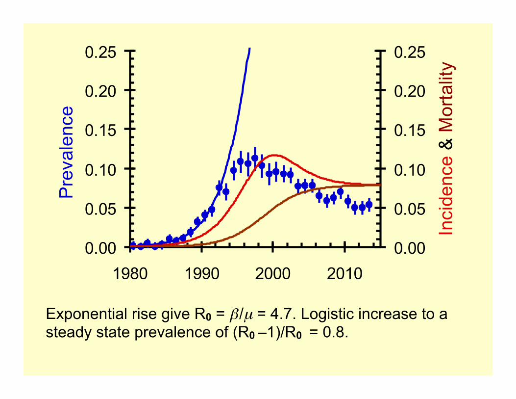
Exponential rise give R0 = β /µ = 4.7. Logistic increase to a steady state prevalence of (R0 –1)/R0 = 0.8.
0.00
0.05
0.10
0.15
0.20
0.25
1980 1990 2000 2010
Pre
vale
nce
0.00
0.05
0.10
0.15
0.20
0.25
Inci
denc
e &
Mor
talit
y

Heterogeneity in risk: 1
Imperial College: A proportion 1/α of the population are at risk; (1 – 1/α) are at no risk
( )* 1 Pβ β α= −
S
β ∗SI I
µI

0.00
0.05
0.10
0.15
0.20
0.25
1980 1990 2000 2010
Pre
vale
nce
0.000
0.005
0.010
0.015
0.020
0.025
Inci
denc
e &
Mor
talit
y
We can now fit the peak prevalence (but not the decline). Model suggest that only 13% of people are at risk of HIV. N.B. If the mortality is 10% per year, it is always 10% of the prevalence. The scales differ by a factor of 10 so the prevalence and mortality curves lie exactly on top of each other.
Heterogeneity: 1
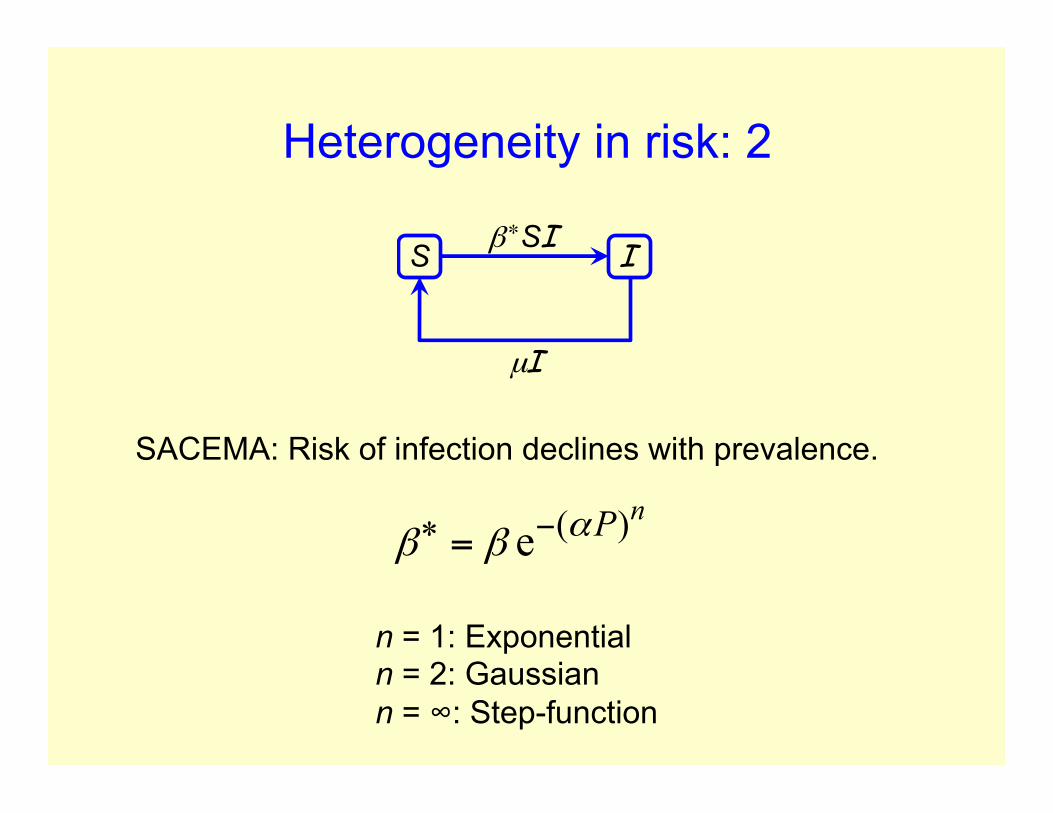
Heterogeneity in risk: 2
SACEMA: Risk of infection declines with prevalence.
( )* enPαβ β −=
n = 1: Exponential n = 2: Gaussian n = ∞: Step-function
S
β ∗SI I
µI

0.00
0.05
0.10
0.15
0.20
0.25
1980 1990 2000 2010
Pre
vale
nce
0.000
0.005
0.010
0.015
0.020
0.025
Inci
denc
e &
Mor
talit
y
0.00
0.05
0.10
0.15
0.20
0.25
1980 1990 2000 2010
Pre
vale
nce
0.000
0.005
0.010
0.015
0.020
0.025
Inci
denc
e &
Mor
talit
y
0.00
0.05
0.10
0.15
0.20
0.25
1980 1990 2000 2010
Pre
vale
nce
0.000
0.005
0.010
0.015
0.020
0.025
Inci
denc
e &
Mor
talit
y
0.00
0.05
0.10
0.15
0.20
0.25
1980 1990 2000 2010
Pre
vale
nce
0.000
0.005
0.010
0.015
0.020
0.025
Inci
denc
e &
Mor
talit
y
All fits are equally good but the implied incidence and the steady state prevalence are quite different. We will use n = 2.
n = 1 n = 2
n = 4 Linear
0.0
0.2
0.4
0.6
0.8
1.0
1980 1990 2000 2010
Ris
k of
infe
ctio
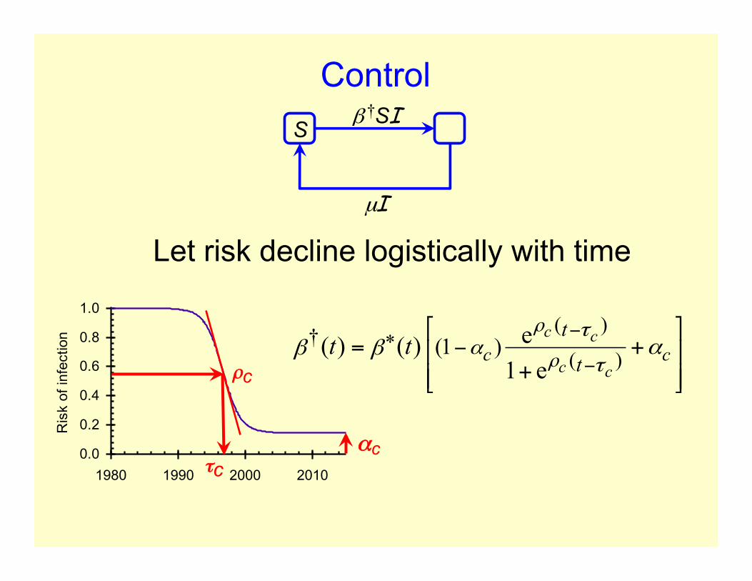
n ( )† *( )(1 ) e( ) ( )
1 e
c c
c cc c
t
tt t
ρ
ρ
τα
ταβ β
−
−−
⎡ ⎤= +⎢ ⎥
+⎢ ⎥⎣ ⎦
Control
αc τc
ρc
Let risk decline logistically with time
S
β †SI
µI
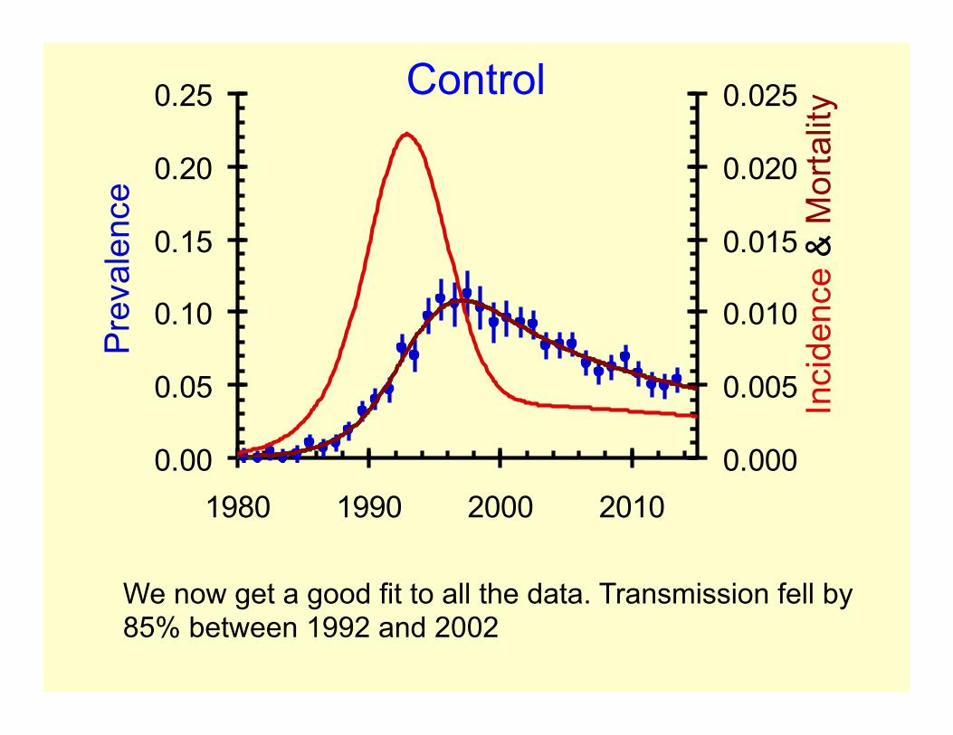
We now get a good fit to all the data. Transmission fell by 85% between 1992 and 2002
0.00
0.05
0.10
0.15
0.20
0.25
1980 1990 2000 2010
Pre
vale
nce
0.000
0.005
0.010
0.015
0.020
0.025
Inci
denc
e &
Mor
talit
yControl
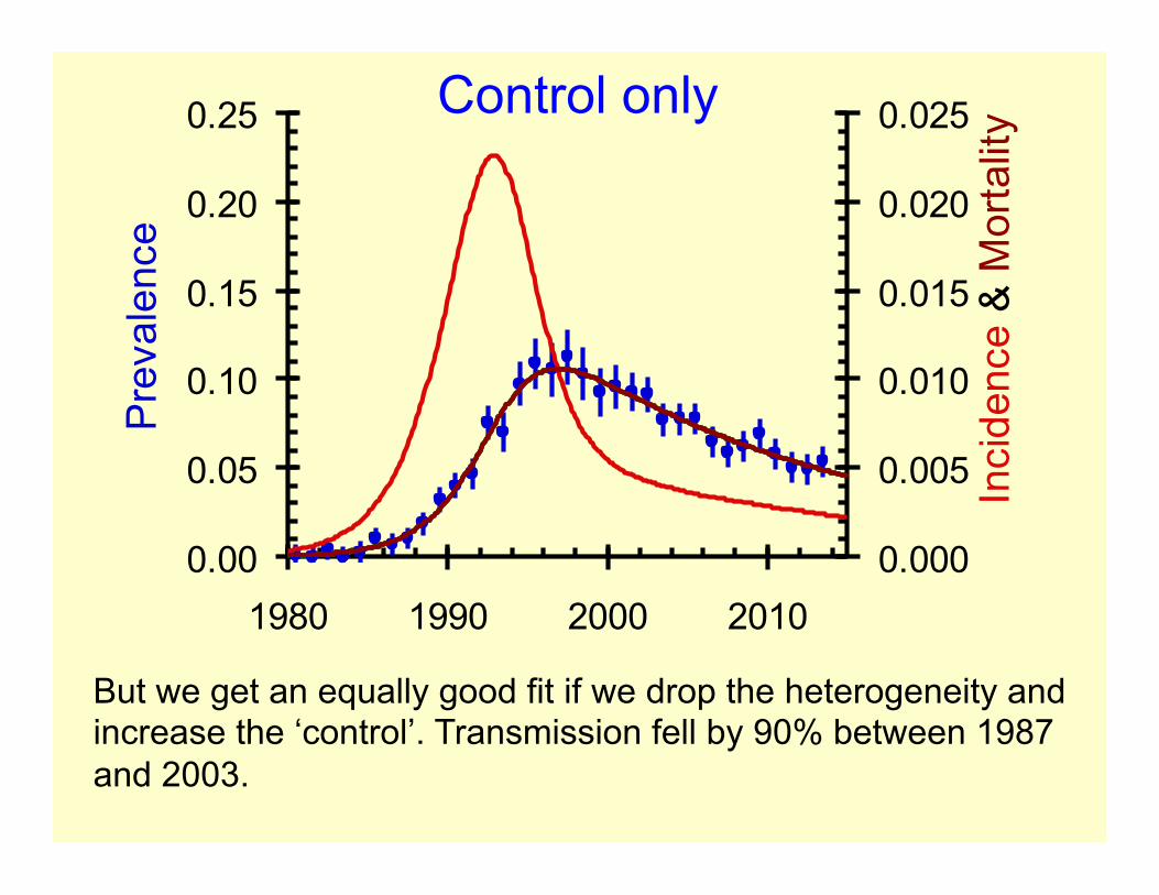
But we get an equally good fit if we drop the heterogeneity and increase the ‘control’. Transmission fell by 90% between 1987 and 2003.
0.00
0.05
0.10
0.15
0.20
0.25
1980 1990 2000 2010
Pre
vale
nce
0.000
0.005
0.010
0.015
0.020
0.025
Inci
denc
e &
Mor
talit
yControl only

0.0
0.2
0.4
0.6
0.8
1.0
1980 1990 2000 2010
Heterogeneity v. control Tr
ansm
issi
on: β
* or
β †
Heterogeneity and control
Control only
Without heterogeneity control has to start 3 years earlier and has to fall further 90% v. 85%.

Survival on HIV follows a Weibull survival curve with a median survival of 10 years and a shape parameter of 2.25. Close to a survival for a Γ-function with a shape parameter of 4. We use four successive compartments for those with HIV.
Weibull survival
0.0
0.2
0.4
0.6
0.8
1.0
30 35 40 45 50Age (years)
Surv
ival
Age 30
S I1 β
†SI ρI I2 I3 I4
ρI ρI
δI4

Mortality now rises about 8 years after the rise in incidence and about 3 years after the rise in prevalence. Weibull survival introduces an important delay.
0.00
0.05
0.10
0.15
0.20
0.25
1980 1990 2000 2010
Pre
vale
nce
0.000
0.005
0.010
0.015
0.020
0.025
Inci
denc
e &
Mor
talit
y
Weibull survival
0.0
0.2
0.4
0.6
0.8
1.0
1980 1990 2000 2010
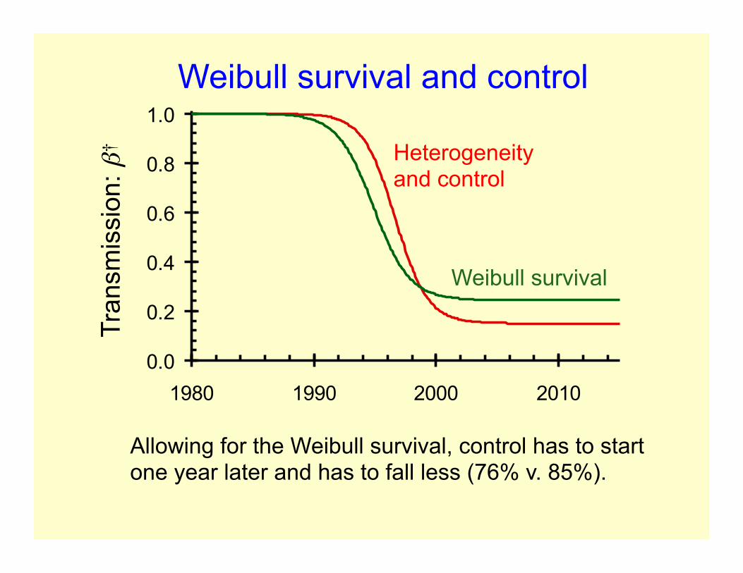
Weibull survival and control Tr
ansm
issi
on: β
† Heterogeneity and control
Weibull survival
Allowing for the Weibull survival, control has to start one year later and has to fall less (76% v. 85%).

Population growth
Separate the birth rate from the death rate and allow people to die from natural causes in each stage. (Birth rate = 3.6% p.a.; death rate = 1.2% p.a.)
S I1
β †SI/N ρI1 β N
δS
I2 I3 I4 ρI2 ρI3
δI1
δI2
δI3
δI4
ρI4

0.00
0.05
0.10
0.15
0.20
0.25
1980 1990 2000 2010
Pre
vale
nce
0.000
0.005
0.010
0.015
0.020
0.025
Inci
denc
e &
Mor
talit
y
Allowing the population to grow (2.4% p.a.) increases incidence and reduces mortality but only slightly.
Population growth
0.0
0.2
0.4
0.6
0.8
1.0
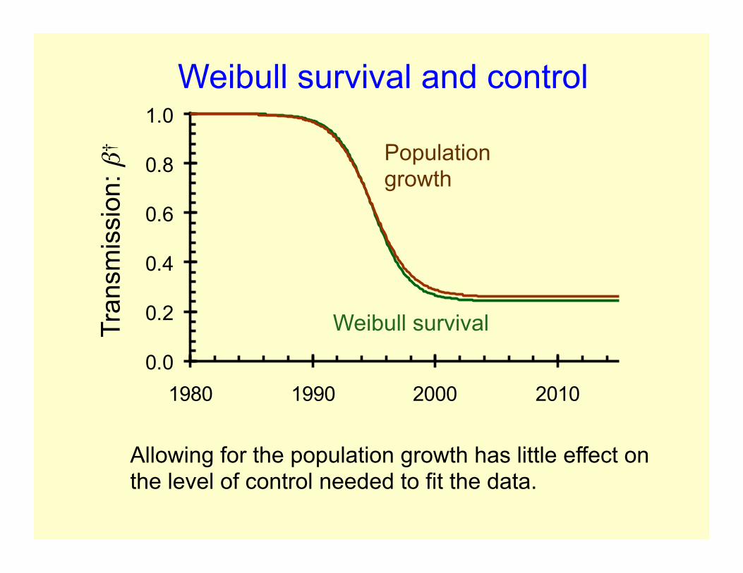
1980 1990 2000 2010
Weibull survival and control Tr
ansm
issi
on: β
† Population growth
Weibull survival
Allowing for the population growth has little effect on the level of control needed to fit the data.
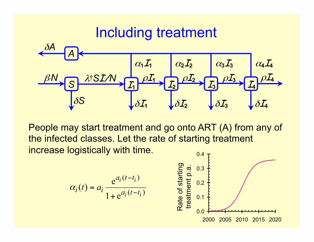
Including treatment
People may start treatment and go onto ART (A) from any of the infected classes. Let the rate of starting treatment increase logistically with time.
S I1 λ†SI/N ρI1 β N
δS
I2 I3 I4 ρI2 ρI3
δI1
δI2
δI3
δI4
A α1I1 α2I2 α3I3 α4I4
δA
ρI4
( )
( )e( )1 e
i i
i i
a t ti i a t tt aα
−
−=
+
Rat
e of
sta
rting
tre
atm
ent p
.a.
0.0
0.1
0.2
0.3
0.4
2000 2005 2010 2015 2020
0.00
0.05
0.10
0.15
0.20
0.25
1980 1990 2000 2010
Pre
vale
nce
0.000
0.005
0.010
0.015
0.020
0.025
Inci
denc
e &
Mor
talit
y
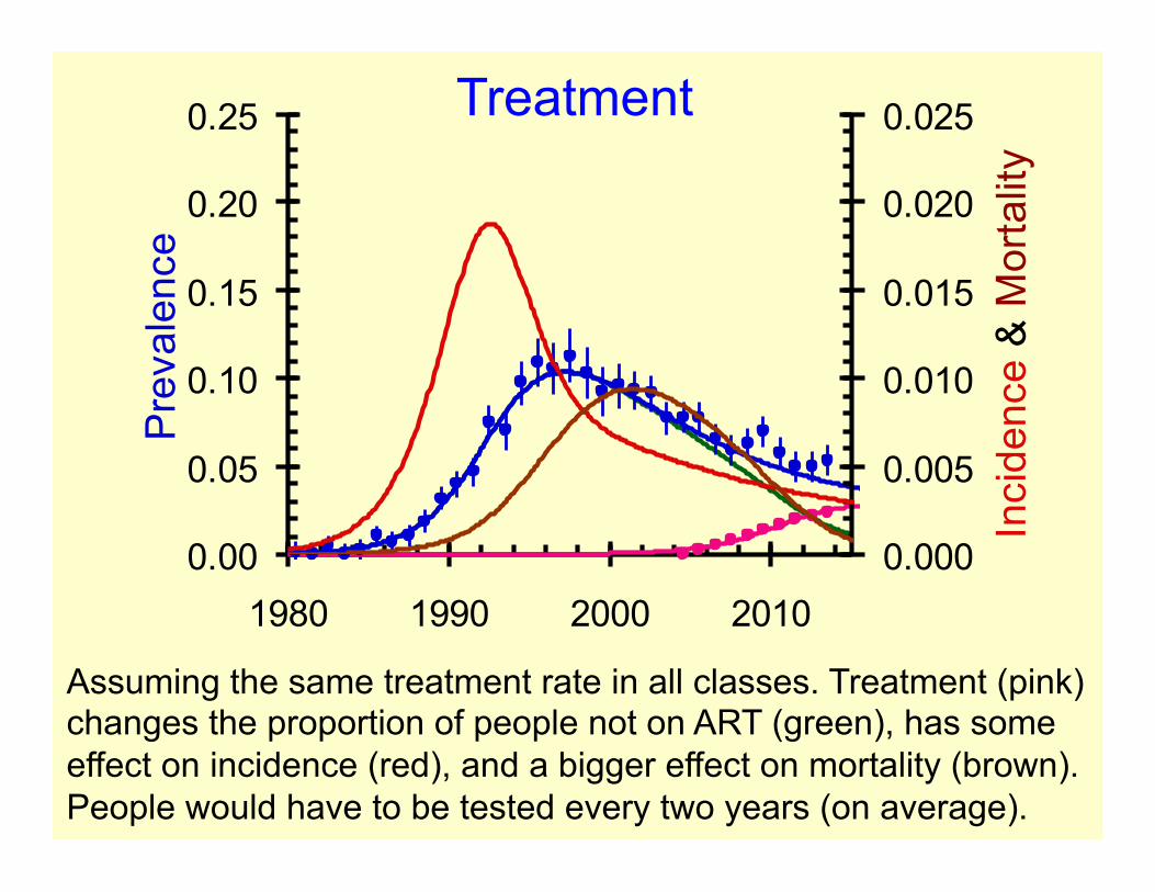
Assuming the same treatment rate in all classes. Treatment (pink) changes the proportion of people not on ART (green), has some effect on incidence (red), and a bigger effect on mortality (brown). People would have to be tested every two years (on average).
Treatment
0.00
0.05
0.10
0.15
0.20
0.25
1980 1990 2000 2010
Pre
vale
nce
0.000
0.005
0.010
0.015
0.020
0.025
Inci
denc
e &
Mor
talit
y
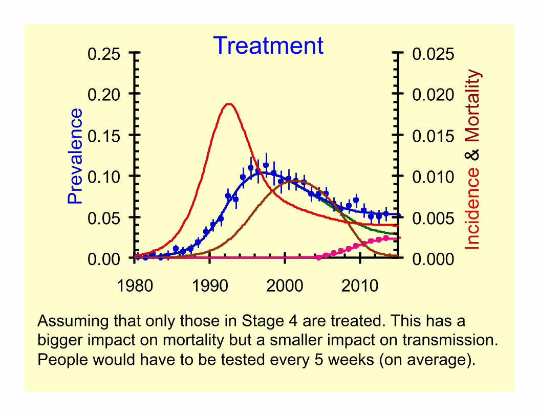
Assuming that only those in Stage 4 are treated. This has a bigger impact on mortality but a smaller impact on transmission. People would have to be tested every 5 weeks (on average).
Treatment

0.00
0.05
0.10
0.15
0.20
0.25
1980 2000 2020 2040
Pre
vale
nce
0.000
0.005
0.010
0.015
0.020
0.025
Inci
denc
e &
Mor
talit
y
Assuming the same treatment rate in all classes will drive the epidemic down slowly
Projections

0.00
0.05
0.10
0.15
0.20
0.25
1980 2000 2020 2040
Pre
vale
nce
0.000
0.005
0.010
0.015
0.020
0.025
Inci
denc
e &
Mor
talit
y
Keeping the same number of people on ART but only treating those in Stage 4 will have a bigger impact on mortality in the short term but will not bring the epidemic under control in the long term.
Projections

0.00
0.05
0.10
0.15
0.20
0.25
1980 1990 2000 2010
Pre
vale
nce
0.000
0.005
0.010
0.015
0.020
0.025
Inci
denc
e &
Mor
talit
y
Uncertainty
With a simple compartmental model we can estimate confidence limits on the the parameters and the fitted curves. (This is an MCMC estimate.)

As people age they can remain uninfectious, be infected, progress with HIV, start treatment, remain on treatment, or fail treatment. They can die of other causes, AIDS, or die on ART.
Demography: The model
Age
Uninfected
Infected
ART
HIV incidence
ART incidence
Failure Background deaths
Births

The computational problem Without demography 9 states (Susceptible 1; Infected 4; ART 4) 16 possible state transitions (20 with treatment failure) 500 time steps (50 years at intervals of 0.1 year) 104 calculations of state transitions With demography Each state can have 1,000 ages (100 years at intervals of 0.1 year) 107 calculations of state transitions In both cases about 6 variable parameters Many more fixed parameters with demography

The computational problem Without demography Solver in Excel converges after about 20 iterations taking about 5 seconds. MCMC estimates of uncertainty require about 1,000 iterations taking about 5 minutes. With demography This is going to take about 5x10⁴ seconds = 14 hours to optimizing the fit and about 5x10⁴ minutes = 35 days to estimate the uncertainty. Is it worth it?

Demography: Fixed parameters 1. Assume that the current age-distribution is a stable age-
distribution. 2. From the overall population growth rate calculate the age-
specific mortality for HIV-negative people. 3. Check that this gives the current stable age-distribution and
population growth rate. 4. Use the age mortality as a function of age for those not on ART.
This declines linearly with age and the survival distribution is Weibull with a shape parameter of 2.25 at all ages.
5. Estimate the (relative) age-specific incidence of infection. 6. Run and fit the demographic equivalent of the model (without
ART). 7. Note that this is still a one-sex model so we are averaging over
a loop of transmission male female male ignoring age-matching of partners and other aspects of the network.

0.00
0.05
0.10
0.15
0.20
0.25
1980 1990 2000 2010
Pre
vale
nce
0.000
0.005
0.010
0.015
0.020
0.025
Inci
denc
e an
d M
orta
lity
Demography
The demography only changes the fits and predictions by a small amount. Incidence declines more quickly, mortality is a little lower (next slide). But both within the uncertainty limits.

0.00
0.05
0.10
0.15
0.20
0.25
1980 1990 2000 2010
Pre
vale
nce
0.000
0.005
0.010
0.015
0.020
0.025
Inci
denc
e &
Mor
talit
y
Repeat of Slide 14.
Population growth
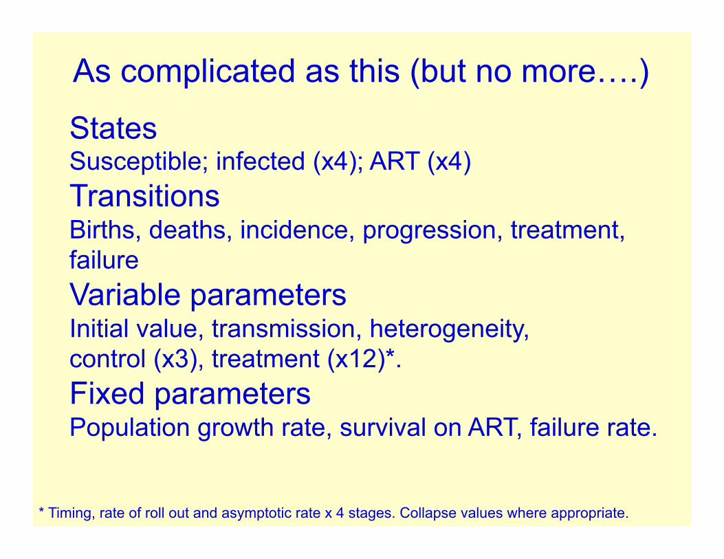
As complicated as this (but no more….)
States Susceptible; infected (x4); ART (x4) Transitions Births, deaths, incidence, progression, treatment, failure Variable parameters Initial value, transmission, heterogeneity, control (x3), treatment (x12)*. Fixed parameters Population growth rate, survival on ART, failure rate.
* Timing, rate of roll out and asymptotic rate x 4 stages. Collapse values where appropriate.

Outputs
Prevalence In each of 4 states off treatment and on treatment with implications for rates of opportunistic infections. Incidence Overall incidence of HIV Starting ART Rate at which people start ART with implications for testing rates. Mortality Death rates off ART.

Interventions
The model indicates the extent to which transmission appears to have fallen pre-ART. Time trends in the levels of different interventions should be used to see if they can reasonably explain the pre-ART decline. Possible interventions include: fewer partners, less age-discordancy, condoms, PreP, PEP, VMMC.