MODELLING CHLORINE DECAY IN DRINKING WATER SUPPLY SYSTEMS · 1" " MODELLING CHLORINE DECAY IN...

1

MODELLING CHLORINE DECAY IN DRINKING WATER SUPPLY SYSTEMS

David Manuel Duarte Figueiredo Instituto Superior Técnico, Lisbon, Portugal, 2014

[email protected]

Abstract: The current work focuses on the analysis of flow hydraulics conditions effect on chlorine residual decay and

on the development of a chlorine residual model in a water supply system from Águas do Algarve utility using EPANET

2. The work involves a literature review about the factors that influence chlorine decay and decay modelling,

experimental studies on a helical pipe rig (friction factor analysis and the study of flow velocity on chlorine decay) and

chlorine residual modelling of Águas do Algarve subsystem. This thesis contributes to a better understanding of the

effect of flow hydraulics conditions on chlorine bulk decay rates and shows that these rates significantly increase with

the flow velocity in turbulent flow for treated waters. An empirical formulation of decay rate that includes the flow

velocity has been developed and can be incorporated in water quality simulators. The simulation of Águas do Algarve

water supply system with first and nth order bulk decay kinetics had similar level of accuracy. However, results have

shown that calibration and validation carried out only based on free chlorine analyzer measurements is not sufficient.

Field measurements are required to calibrate and validate the models.

Keywords: chlorine residual modelling, chlorine decay, drinking water quality, water distribution systems.

1 INTRODUCTION

Chlorine residual is used worldwide as a hygienic

barrier in drinking water systems. Chlorine

concentration decreases as the water travels

throughout the systems, where its levels must be

enough to assure the disinfectant effectiveness. As the

formation of toxic disinfection by-‐products increases

with chlorine concentration, this must be maintained in

drinking water within a quite narrow range, usually

between 0.2 and 1.0 mg/L (WHO, 2011) and 0.2 and 0.6

mg/L according to Portuguese law (Decreto-‐Lei

n.º 306/2007 de 27 de Agosto). However, the Annual

Report of the Portuguese Water and Waste Regulator

reveals that 45% of analysed samples have a chlorine

residual insufficient to ensure hygienic barrier.

Chlorine decay models are important tools for the

management of disinfectant concentration in drinking

water systems, particularly for dosage optimization and

chlorination facilities location. Despite the considerable

amount of research developed in the last twenty years

(Clark, 2011; Powell et al., 2000a; Rossman et al.,

1994), chlorine decay phenomena and the factors that

influence them are still being studied. Most water

quality simulators describe chlorine decay by the sum

of two groups of chemical reactions in which chlorine is

consumed: reactions in the water (bulk decay) and at

the pipes‘ internal surface (wall decay). Bulk decay is

due to reactions of chlorine with compounds dissolved

in the water, mainly those composing the Natural

Organic Matter (NOM) and, to a minor extent, with

inorganic compounds, like reduced iron and

manganese forms (Powell et al., 2000a). The most

widely used kinetic models in water supply systems

simulation is the first order model (Clark &

Sivaganesan, 2002):

Clb Cl

dCK C

dt= − (1)

where ClC is chlorine concentration, t is time, and bK

is the bulk decay coefficient (or bulk reaction rate

constant). The nth order bulk decay kinetic model with

2

respect to chlorine is described by the following

equation (Powell et al., 2000b):

nClb Cl

dCK C

dt= − (2)

where the n is the order of the reaction with respect

to chlorine. The decay coefficient is commonly

determined through the laboratory bottle test (Powell

et al., 2000a).

Wall decay is particularly important in systems with

metal pipes (Hallam et al., 2002) owing to chlorine

consumption in corrosion processes. Biofilm and

sediments may also play a significant role in chlorine

decay at the pipes’ wall. Except in corroding iron pipes,

bulk decay is responsible for most of chlorine

consumption, having the wall demand a much smaller

contribution to the overall chlorine decay (Kiene et al.,

1998).

Wall decay may also be described by a first order

kinetic model (Rossman et al., 1994):

(3)

where wk is the wall decay coefficient (or wall reaction

rate constant), fk is a mass transfer coefficient

(velocity dependent) and D is the pipe diameter. The

wall kinetic coefficient cannot be experimentally

determined and is usually calibrated in order to fit

calculated to measured chlorine concentrations.

Chlorine decay rates depend on the system operational

conditions, such as water temperature, initial chlorine

concentration, on the type and concentration of NOM

(Brown et al., 2011; Hallam et al., 2003; Powell et al.,

2000a) and flow velocity (Hallam et al., 2002; Menaia

et al., 2003).

An accurate chlorine decay model requires a suitable

kinetic model (Fisher et al., 2011; Powell et al., 2000b)

that is able to describe chlorine decay as a function of

the influencing factors.

The temperature effect on chemical reaction rates

coefficients is generally described by the empirical

Arrhenius equation:

( )aE RTk Ae−= (4)

where k is the reaction rate coefficient, A is the

frequency factor, aE is the activation energy, R is the

ideal gas constant (8.31 J mol-‐1 K-‐1) and T is the

temperature (Monteiro et al., 2014). The Arrhenius

parameters ( A and aE ) are specific of each chemical

reaction.

An increase in bulk decay coefficient with Reynolds

number was reported by Menaia et al. (2003) and

Ramos et al. (2010).

According to Menaia et al. (2003), water flow velocity

effect on first order chlorine bulk decay coefficient can

be described by:

Kb

d = Kb 1+ bU D( ) (5)

Where dbK is the bulk decay coefficient at velocity U ,

bK is the bulk decay coefficient at stagnant conditions

and b is an adjustable parameter (103.20 m-‐2 s for the

tested conditions). Ramos et al. (2010) also observed a

significant increase of parallel first order kinetic

constants with increasing Reynolds number and

described it with a linear function. The parameters in

Equation 5 are related to tested waters temperature

and NOM reactivity towards chlorine, thus hindering a

straightforward implementation of these equations in

chlorine residual modelling. Additionally, the testing

conditions used by Menaia et al. (2003) and Ramos et

al. (2010) do not reflect real conditions in drinking

water networks. Those authors used commercial humic

acids as surrogate for NOM at relatively high

concentrations (5 mg C/L as Total Organic Carbon).

The aim of this work is the study of the effect of

hydraulic conditions on chlorine bulk decay coefficient

in treated waters and to develop an empirical

formulation for bK as a function of hydraulic

parameters. Additionally, this work intended to

contribute to the implementation of residual chlorine

modeling in a Portuguese water transmission system

dCCl

dt= −

4k f kwCCl

D(k f + kw )

3

and to identify the major difficulties and uncertainties

in water quality modelling.

2 EXPERIMENTAL SETUP AND

PROCEDURES

Two sets of experiments were performed in a

laboratory pipe rig. The first tests aimed at determining

the flow velocity in the pipe rig for the different

operation conditions for pipe friction analysis. The

second set of tests was performed in order to analyse

the effect of hydraulic conditions on chlorine decay

bulk coefficient.

2.1 Pipe rig description

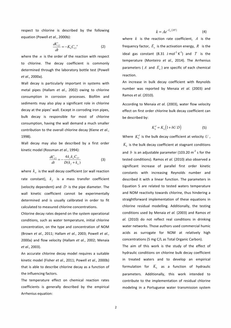
The pipe rig (Figure 1), assembled in the Laboratory of

Hydraulics and Environment of Instituto Superior

Técnico, is a helical pipe closed loop of high-‐density

polyethylene (HDPE) with about 100 m long and 32 mm

diameter. The system was about 2 m high and included

a recirculation pump (Filtra N 24D, KSB) connected to a

variable-‐frequency drive, a 4 L capacity standpipe on

top, a sampling port, a 15 cm long transparent

polyvinyl chloride (PVC) pipe branch and a valve on the

bottom to fill and to drain the system. All fittings were

made of PVC and the pump internal materials were

plastic.

Figure 1 – Pipe rig.

The system operates in a closed loop and reproduces a

hydraulic pressure system consisting of a long pipe

without branching.

2.2 Flow velocity estimation

Tracer tests were performed at 17 flows with

demineralized water. For each test, sodium chloride

was injected with a syringe at the beginning of the

HDPE pipe. The conductivity was continuously

measured with a conductivity probe placed at the end

of the HDPE pipe. The tracer time between the

injection section and the conductivity probe was

measured, as well as the water temperature. The

piezometric head variation between two sections in the

pipe was measured using two piezometers installed in

the circuit.

2.3 Chlorine decay tests

For each experiment, 80 L of Tavira Water Treatment

Plant final water were chlorinated with sodium

hypochlorite (ca. 1.0 mg/L) in a plastic tank and

immediately pumped into the pipe rig until the system

was completely filled with water. Trapped air was

thoroughly eliminated. When no air bubbles were

observed, water samples were collected for initial

chlorine concentration measurement and to

completely fill twelve amber glass 100 mL bottles.

Then, loop water flow velocity was set (Table 1) and

kept steady for several days. Chlorine concentration in

the pipe rig water was monitored by collecting and

analysing samples with the N,N-‐diethyl-‐p-‐

phenyldiamine (DPD) method, using a

spectrophotometer (Dr. Lange, Cadas 50). The water

temperature was monitored with a digital

thermometer inserted in the pipe. The bottles were

placed in a cardboard box, to protect from light, next to

the pipe rig at the same ambient temperature. Chlorine

concentration and temperature in the bottles water

were measured at the same time intervals as for the

pipe rig samples. Tests lasted until chlorine

concentration in rig pipe water decreased to bellow the

method measurement limit (0.1 mg/L) or for 7 days.

Experiments comprised five different flow rates for

4

tested water (Table 1). One additional experiment with

chlorinated demineralized water was performed at

1.07 m/s to evaluate pipe´s wall contribution to overall

chlorine decay. Decay tests were done at Reynolds

numbers within the range from 4089 to 16160, hence

included both laminar and turbulent flow regimes.

3 FRICTION RESISTANCE IN HELICAL PIPES

3.1 Friction factors

In an incompressible steady flow, piezometric head

variation between two sections in the pipe it is the

head loss between those sections. The unit headloss

( J ) for a pipe with constant cross section can be

determined by Darcy-‐Weisbach equation:

J = f U2

2gD (6)

where f is the Darcy friction factor, g is the gravity

acceleration and D is the pipe inner diameter. The

friction factor formulation varies with flow regimes and

pipe configuration. In laminar flows in straight pipes,

Hagen-‐Poiseuille law can be used:

f = 64Re

(7)

where Re is the Reynolds number. In turbulent flows

in smooth straight pipes, the Karman-‐Prandtl semi-‐

empirical formula is used:

1f 0.5

= −2 log 2.51Re f 0.5

⎛⎝⎜

⎞⎠⎟ (8)

Ito (1959) has study the friction factors formulas for

flows in helical pipes. From his results, the friction

factor for laminar flow is given by:

f = 64Re

21.5De(1.56 + logDe)5.73

(9)

and for turbulent flow is given by:

f = 0.304Re−0.25+ 0.029 Ddc

⎛⎝⎜

⎞⎠⎟

0.5

(10)

where dc is the curvature diameter and De is the

Dean number ( De = Re D dc( )0.5 ).

In helical pipes, the laminar to turbulent flow transition

occurs at a higher Reynolds number. Srinivasan et al.

(1970) indicate that the flow transition occurs around

the critical Reynolds number,Rec :

Rec = 2100 1+12Ddc

⎛⎝⎜

⎞⎠⎟

0.28⎡

⎣⎢⎢

⎤

⎦⎥⎥ (11)

3.2 Experimental friction factor formulations

The specific Rec of this pipe rig is 6140 (for D = 0.0264

m and dc = 1.027 m).

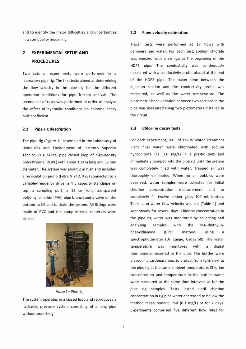
The experimental friction factor for 17 tests of the first

set were calculated and were compared with existing

formulations for laminar (Figure 2) and for turbulent

flows (Figure 3).

Figure 2 – Comparison of existing formulations and

experimental results for turbulent flow.

Figure 3 – Comparison of existing formulations and

experimental results for laminar flow.

0,00

0,05

0,10

0,15

0,20

500 1500 2500 3500 4500

fric

tion

fact

or

Re

Experimental

Hagen-‐Poiseuille

Ito (1959) laminar flow

Empirical formulanon

0,02

0,03

0,04

0,05

6000 16000 26000 36000

fric

tion

fact

or

Re

Experimental Karman-‐Prandtl smooth pipes Ito (1959) turbulent flow Empirical formulanon

𝑓 = 22.246 Re-0.78 R2=0.96

𝑓=0.1115 Re-0.14 R2=0.98

5

Results have shown that, in helical pipes, the friction is

higher than in straight pipes for both laminar and

turbulent flows. However, the experimental results of

the friction factor for Re < 11 000 (in turbulent flow) were lower than the ones for straight pipes.

Empirical formulations for friction factor of the pipe rig

flow were developed for laminar flow:

f = 22.246Re−0,78 (12)

and for turbulent flow:

f = 0.1115Re−0.14 (13)

3.3 Flow velocity estimation

An empiric formulation were determined to estimate

the flow velocity in the pipe rig with unit headloss ( J )

through the Equations (12) and (13).

The flow velocity for laminar flow can be estimated by:

U = 2gJD1.78

22.246ν 0.78

⎛⎝⎜

⎞⎠⎟

0.82

(14)

and for turbulent flow by:

U = 2gJD1.14

0.1115ν 0.14

⎛⎝⎜

⎞⎠⎟

0.54

(15)

The unit headloss ( J ) is determined by the ratio of the

measured piezometric head variation in two

piezometers installed in the pipe rig and the distance

( L ) between them.

4 HYDRAULIC CONDITIONS EFFECT ON

CHLORINE DECAY

Decay test with demineralized water (blank tests)

showed only minor decay of chlorine concentration

through time, both in the pipe rig and in the bottles. A

simple first order kinetic model was used to describe

chlorine decay in demineralized water bottle tests and

estimate bulk decay coefficient. Chlorine decay in the

pipe rig in the blank test was modelled using first order

(0.0015 h-‐1) and calibrating the wall decay

coefficient by minimizing the sum of the squared

residuals between measured and modelled values. A

first order kinetic model was assumed for wall decay. A

rather low value of 2.6x10-‐06 m/h was found for ,

which is in accordance with Clark (2011), who states

the low contribution of plastic pipes for chlorine decay.

A nth order kinetic model (n = 2) was used and

accurately described chlorine decay in the bottles with

the tested water (Table 1). Coefficient of determination

(R2) and Root Mean Squared Error (RMSE) assessed

goodness of fit of the model to experimental data.

Determined bulk decay coefficients varied between

0.020 and 0.067 L/mg/h due to differences in water

temperature and possibly due to variations in water

quality. At the smallest water flow velocity tested (0.15

m/s), chlorine decayed in the pipe at the same rate as

in the bottles. For all the other tested velocities,

chlorine decayed faster in the pipe rig, which is in

accordance with Menaia et al. (2003) and Ramos et al.

(2010) findings.

Chlorine decay in the pipe rig in each experiment was

modelled by the usual “bulk + wall” approach and using

from bottle tests and previously determined

from blank test:

dCCl

dt= −KbCCl

2 − 4D

kf kw(k f + kw )

CCl (16)

The obtained RMSE (Table 1) is relatively high (above

0.06 mg / L) and shows a tendency to increase with

water flow velocity, as higher values were obtained

with higher tested velocities (0.52 and 0.61 m/s).

Apparently, there is an increasing inability of the model

to describe chlorine decay in the pipe as the water flow

velocity increases. Hence, a new modelling approach

was developed in order to incorporate flow velocity

effect on . Bulk decay coefficient in Equation (16)

was replaced by an analogous coefficient, determined

in dynamic flow conditions, :

dCCl

dt= −Kb

dCCl2 − 4

Dkf kw

(k f + kw )CCl (17)

The new coefficient was determined by fitting Equation

(17) to experimental results of each test. In order to

Kb

kw

Kb kw

Kb

Kbd

6

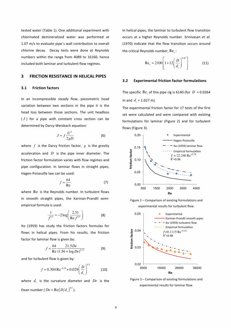
compare the obtained values with from bottle

tests, the ratio of the two coefficients was computed

(Table 2). Results have shown that the ratio increased

with flow velocity (Figure 4) and that bulk decay

coefficient in turbulent flow conditions may double its

value. These results are in agreement with Menaia et

al. (2003) and Ramos et al. (2010) who observed an

increase in bulk decay coefficient with flow velocity and

Reynolds number, respectively.

A linear relationship between the ratio Kbd Kb and

Reynolds number (Figure 4) was also developed:

Kbd = Kb 1×10

−4 Re+ 0.62( ) (18)

A similar equation was derived between the ratio

Kbd Kb and flow velocity:

Kbd = Kb 2.57U + 0.62( ) (19)

Figure 4 – Ratio 𝑲𝒃

𝒅 𝑲𝒃 variation with Reynolds number.

Equations (18) and (19) describe hydraulic conditions

effect on bulk decay coefficient in the test rig. The

equations’ parameters are probably a characteristic of

the tested water and of the pipe system configuration.

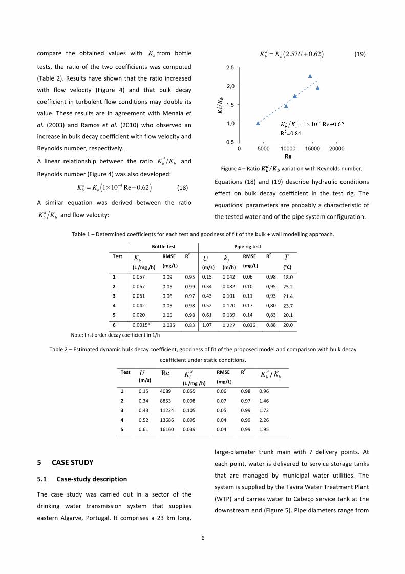
Table 1 – Determined coefficients for each test and goodness of fit of the bulk + wall modelling approach.

Bottle test Pipe rig test

Test

(L /mg /h)

RMSE

(mg/L)

R2

(m/s)

(m/h)

RMSE

(mg/L)

R2

(°C)

1 0.057 0.09 0.95 0.15 0.042 0.06 0,98 18.0

2 0.067 0.05 0.99 0.34 0.082 0.10 0,95 25.2

3 0.061 0.06 0.97 0.43 0.101 0.11 0,93 21.4

4 0.042 0.05 0.98 0.52 0.120 0.17 0,80 23.7

5 0.020 0.05 0.98 0.61 0.139 0.14 0,83 20.1

6 0.0015* 0.035 0.83 1.07 0.227 0.036 0.88 20.0

Note: first order decay coefficient in 1/h

Table 2 – Estimated dynamic bulk decay coefficient, goodness of fit of the proposed model and comparison with bulk decay

coefficient under static conditions.

Test U (m/s)

Re Kbd

(L /mg /h)

RMSE

(mg/L)

R2

Kbd / Kb

1 0.15 4089 0.055 0.06 0.98 0.96

2 0.34 8853 0.098 0.07 0.97 1.46

3 0.43 11224 0.105 0.05 0.99 1.72

4 0.52 13686 0.095 0.04 0.99 2.26

5 0.61 16160 0.039 0.04 0.99 1.95

5 CASE STUDY

5.1 Case-‐study description

The case study was carried out in a sector of the

drinking water transmission system that supplies

eastern Algarve, Portugal. It comprises a 23 km long,

large-‐diameter trunk main with 7 delivery points. At

each point, water is delivered to service storage tanks

that are managed by municipal water utilities. The

system is supplied by the Tavira Water Treatment Plant

(WTP) and carries water to Cabeço service tank at the

downstream end (Figure 5). Pipe diameters range from

Kb

0,5

1,0

1,5

2,0

2,5

0 5000 10000 15000 20000 Re

Kb U k f T

𝑲𝒃𝒅𝑲𝒃

⁄

7

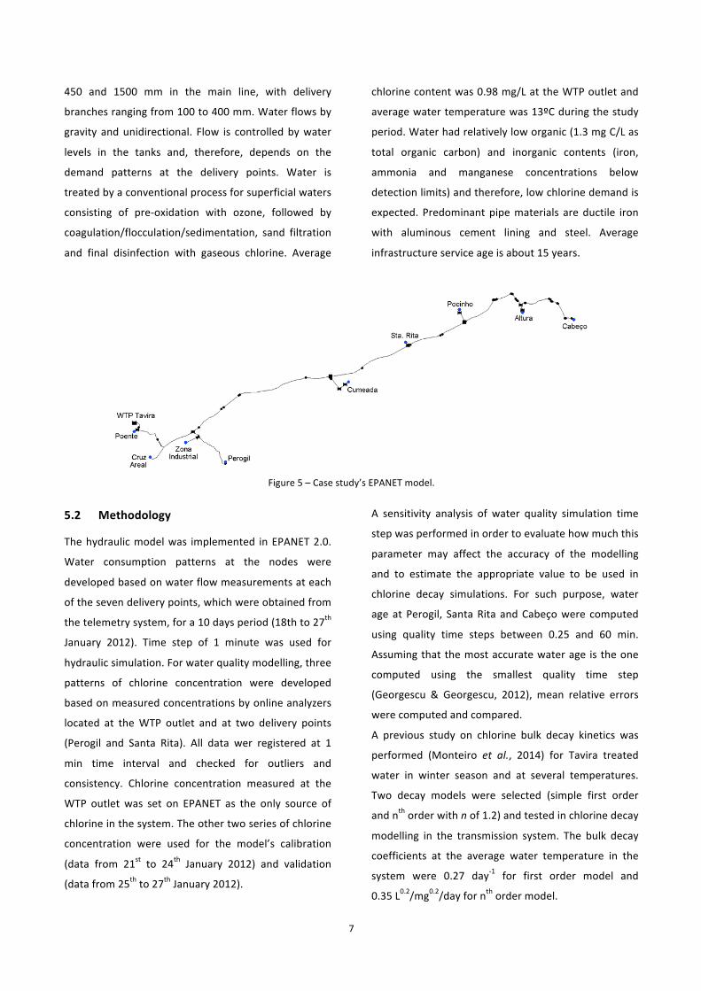
450 and 1500 mm in the main line, with delivery

branches ranging from 100 to 400 mm. Water flows by

gravity and unidirectional. Flow is controlled by water

levels in the tanks and, therefore, depends on the

demand patterns at the delivery points. Water is

treated by a conventional process for superficial waters

consisting of pre-‐oxidation with ozone, followed by

coagulation/flocculation/sedimentation, sand filtration

and final disinfection with gaseous chlorine. Average

chlorine content was 0.98 mg/L at the WTP outlet and

average water temperature was 13ºC during the study

period. Water had relatively low organic (1.3 mg C/L as

total organic carbon) and inorganic contents (iron,

ammonia and manganese concentrations below

detection limits) and therefore, low chlorine demand is

expected. Predominant pipe materials are ductile iron

with aluminous cement lining and steel. Average

infrastructure service age is about 15 years.

Figure 5 – Case study’s EPANET model.

5.2 Methodology

The hydraulic model was implemented in EPANET 2.0.

Water consumption patterns at the nodes were

developed based on water flow measurements at each

of the seven delivery points, which were obtained from

the telemetry system, for a 10 days period (18th to 27th

January 2012). Time step of 1 minute was used for

hydraulic simulation. For water quality modelling, three

patterns of chlorine concentration were developed

based on measured concentrations by online analyzers

located at the WTP outlet and at two delivery points

(Perogil and Santa Rita). All data wer registered at 1

min time interval and checked for outliers and

consistency. Chlorine concentration measured at the

WTP outlet was set on EPANET as the only source of

chlorine in the system. The other two series of chlorine

concentration were used for the model’s calibration

(data from 21st to 24th January 2012) and validation

(data from 25th to 27th January 2012).

A sensitivity analysis of water quality simulation time

step was performed in order to evaluate how much this

parameter may affect the accuracy of the modelling

and to estimate the appropriate value to be used in

chlorine decay simulations. For such purpose, water

age at Perogil, Santa Rita and Cabeço were computed

using quality time steps between 0.25 and 60 min.

Assuming that the most accurate water age is the one

computed using the smallest quality time step

(Georgescu & Georgescu, 2012), mean relative errors

were computed and compared.

A previous study on chlorine bulk decay kinetics was

performed (Monteiro et al., 2014) for Tavira treated

water in winter season and at several temperatures.

Two decay models were selected (simple first order

and nth order with n of 1.2) and tested in chlorine decay

modelling in the transmission system. The bulk decay

coefficients at the average water temperature in the

system were 0.27 day-‐1 for first order model and

0.35 L0.2/mg0.2/day for nth order model.

8

Chlorine residual in the transmission system was firstly

simulated assuming that only bulk decay was occurring.

Then, a wall decay coefficient was iteratively calibrated

by minimizing the sum of the squared differences

between simulated and measured chlorine

concentrations at the two nodes where online

analyzers were located. Wall decay was modelled

assuming a first order model, as the pipe materials are

predominantly of low reactivity (lined ductile iron). A

single wall coefficient was calibrated for the whole

system since over 85% of the pipes are of the same

material and of identical service age.

5.3 Water age sensitivity analysis

Results have shown that water age relative errors

significantly increase with quality time step (Figure 6)

for the three locations. Relative error was about 6 to

10% when quality time step was set to 5 min, which is

the recommended value on EPANET manual (Rossman,

2000). When the quality time step is set to 1 min or

less, low mean errors of approximately 1% (Figure 6)

were obtained. Therefore, considering the best

compromise between simulation time and accuracy of

the model, all henceforward chlorine decay simulations

were performed using 1 min as quality time step. These

results have shown that the Lagrangian time-‐driven

simulation method used by EPANET is sensitive to the

calculation step and that the choice of quality time step

is extremely important when implementing a water

quality model.

Figure 6 –Water age relative error for each tested quality

time step at Perogil, Santa Rita and Cabeço delivery points.

5.4 Chlorine decay modelling

Modelling chlorine residuals assuming that the pipes’

walls would not have a significant demand has led to

poor correlations (R2 less than 0.85) between

computed and measured chlorine concentrations at

Perogil and Santa Rita delivery points, whichever bulk

decay kinetics were used (Figure 7a). In these

simulations, both models overestimated chlorine

concentrations and only a minor difference is noticed

between the two tested models. These results suggest

that, on one hand, bulk decay is probably not being

accurately described, since flow velocity effect was not

taken into account in the modelling, and, on the other

hand, that wall demand is an important part of chlorine

decay in this system and must be incorporated in the

modelling as well.

By calibrating the wall decay coefficient, better

correlations were obtained (R2 of about 0.93) between

measured and computed values, as observed by

Vasconcelos et al (1997) (Figure 7b). Calibrated

were 0.035 and 0.022 m/day when using bulk decay

kinetics of first and nth order, respectively. Estimated

wall decay coefficient was higher when the first order

kinetic model was used for bulk decay description,

which is due to the higher discrepancies between this

model’s computed chlorine concentrations and

measured ones. This suggests that uncertainties in

bulk decay simulations are being partially incorporated

in the calibrated wall decay coefficient, thus in

accordance with Fisher et al. (2011) findings. RMSE of

the 0.03 mg/L whichever bulk decay kinetics are used,

which is lower than the precision of the most widely

used chlorine concentration measurement method

(0.05 mg/L for HACH colorimeters). Therefore, the

models were considered sufficiently accurate.

0,0

0,5

1,0

1,5

2,0

2,5

0 20 40 60

Rel

ativ

e er

ror

Water quality time step (min)

Cabeço Perogil Sta Rita

kw

9

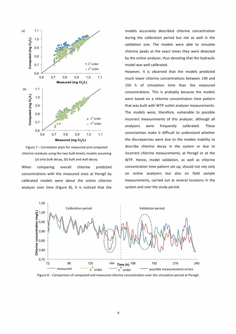
Figure 7 – Correlation plots for measured and computed

chlorine residuals using the two bulk kinetic models assuming

(a) only bulk decay, (b) bulk and wall decay.

When comparing overall chlorine predicted

concentrations with the measured ones at Perogil by

calibrated models were about the online chlorine

analyzer over time (Figure 8), it is noticed that the

models accurately described chlorine concentration

during the calibration period but not as well in the

validation one. The models were able to simulate

chlorine peaks at the exact times they were detected

by the online analyzer, thus denoting that the hydraulic

model was well calibrated.

However, it is observed that the models predicted

much lower chlorine concentrations between 140 and

150 h of simulation time than the measured

concentrations. This is probably because the models

were based on a chlorine concentration time pattern

that was built with WTP outlet analyzer measurements.

The models were, therefore, vulnerable to possible

incorrect measurements of this analyzer, although all

analyzers were frequently calibrated. These

uncertainties make it difficult to understand whether

the discrepancies were due to the models inability to

describe chlorine decay in the system or due to

incorrect chlorine measurements, at Perogil or at the

WTP. Hence, model validation, as well as chlorine

concentration time pattern set up, should not rely only

on online analyzers but also on field sample

measurements, carried out at several locations in the

system and over the study period.

Figure 8 – Comparison of computed and measured chlorine concentration over the simulation period at Perogil.

0,6

0,7

0,8

0,9

1,0

1,1

0,6 0,7 0,8 0,9 1,0 1,1

Com

pute

d (m

g C

l 2/L)

Measured (mg Cl2/L)

0,6

0,7

0,8

0,9

1,0

1,1

0,6 0,7 0,8 0,9 1,0 1,1

Com

pute

d (m

g C

l 2/L)

Measured (mg Cl2/L)

0,75

0,80

0,85

0,90

0,95

1,00

1,05

72 96 120 144 168 192 216 240

Chl

orin

e co

ncen

trat

ion

(mg/

L)

Time (h)

(a)

(b)

1st order

nth order

1st order

nth order

Calibration period Validation period

measured

possible measurements errors

1st order n

th order

10

6 CONCLUSIONS

Chlorine bulk decay coefficient of treated water

significantly increases with water flow velocity for

turbulent conditions. A linear relationship between

bulk decay coefficient at turbulent conditions and

Reynolds number was developed. Such expression

might be incorporated in chlorine decay models,

making use of EPANET-‐MSX potential. Using kb from

bottle tests for modelling chlorine in water supply

systems is likely to result in models of low accuracy.

Including the effect of water flow velocity will reduce

the importance of wall demand on overall chlorine

decay.

When modelling chlorine residual in water supply

systems, relying on online analyzer’s measurements

can be of great advantage, although these data must

be validated and complemented with field sample

measurements, particularly at the source point of

chlorinated water in the system. Additionally, for

greater accuracy, chlorine residual simulations on

EPANET must be performed using small quality time

steps.

REFERENCES

Brown, D., Bridgeman, J., West, J.R., 2011. Predicting chlorine decay and THM formation in water supply systems. Rev. Environ. Sci. Bio/Technology 10, 79–99.

Clark, R.M., 2011. Chlorine fate and transport in drinking water distribution systems: Results from experimental and modeling studies. Front. Earth Sci. 5, 334–340.

Clark, R.M., Sivaganesan, M., 2002. Predicting chlorine residuals in drinking water: Second order model. J. Water Resour. Plan. Manag. 128, 152–161.

Fisher, I., Kastl, G., Sathasivan, A., 2011. Evaluation of suitable chlorine bulk-decay models for water distribution systems. Water Res. 45, 4896–4908.

Georgescu, A.-M., Georgescu, S.-C., 2012. Chlorine concentration decay in the water distribution system of a town with 50000 inhabitants. Univ. Politeh. Bucharest Sci. Bull. Ser. D Mech. Eng. 74, 103–114.

Hallam, N.B., Hua, F., West, J.R., Forster, C.F., Simms, J., 2003. Bulk Decay of Chlorine in Water Distribution Systems. J. Water Resour. Plan. Manag. 129, 78–81.

Hallam, N.B., West, J.R., Forster, C.F., Powell, J.C., Spencer, I., 2002. The decay of chlorine associated with the pipe wall in water distribution systems. Water Res. 36, 3479–3488.

Itō, H., 1959. Friction Factors for Turbulent Flow in Curved Pipes. J. Basic Eng. Trans. ASME, Ser. D 81, 123–134.

Kiene, L., Lu, W., Levi, Y., 1998. Relative importance of the phenomena responsible for chlorine decay in drinking water distribution systems. Water Sci. Technol. 38, 219–227.

Menaia, J.F., Coelho, S.T., Lopes, A., Fonte, E., Palma, J., 2003. Dependency of bulk chlorine decay rates on flow velocity in water distribution networks. Water Sci. Technol. Water Supply 3, 209–214.

Monteiro, L.P., Figueiredo, D., Dias, S., Freitas, R., Covas, D., Menaia, J.F., Coelho, S.T., 2014. Modeling of chlorine decay in drinking water supply systems using EPANET MSX. Procedia Eng. 70, 1192–1200.

Powell, J.C., Hallam, N.B., West, J.R., Forster, C.F., Simms, J., 2000a. Factors which control bulk chlorine decay rates. Water Res. 34, 117–126.

Powell, J.C., West, J.R., Hallam, N.B., Forster, C.F., Simms, J., 2000b. Performance of Various Kinetic Models for Chlorine Decay. J. Water Resour. Plan. Manag. 126, 13–20.

Ramos, H.M., Loureiro, D., Lopes, A., Fernandes, C., Covas, D., Reis, L.F., Cunha, M.C., 2010. Evaluation of Chlorine Decay in Drinking Water Systems for Different Flow Conditions: From Theory to Practice. Water Resour. Manag. 24, 815–834. doi:10.1007/s11269-009-9472-8

Rossman, L.A., 2000. EPANET 2 Users Manual. Cincinnati, OH.

Rossman, L.A., Clark, R.M., Grayman, W.M., 1994. Modeling chlorine residuals in drinking-water distribution systems. J. Environ. Eng. 120, 803–820.

Srinivasan, P.S., Nandapurkar, S.S., Holland, F.A., 1970. Friction factors for coils. Trans. Inst. Chem. Eng 48, T156–T161.

Vasconcelos, J.J., Rossman, L.A., Grayman, W.M., Boulos, P.F., Clark, R.M., 1997. Kinetics of chlorine decay. J. – Am. Water Work. Assoc. 89, 54–65.

World Health Organization, 2011. Guidelines for drinking-water quality, 4th ed. ed. Geneva.

MODELLING CHLORINE DECAY IN DRINKING WATER SUPPLY SYSTEMS · 1" " MODELLING CHLORINE DECAY IN...

Documents

Transcript of MODELLING CHLORINE DECAY IN DRINKING WATER SUPPLY SYSTEMS · 1" " MODELLING CHLORINE DECAY IN...