Modeling high-dimensional natural inflows for stochastic-dynamic optimization

Workshop on Hydro Scheduling in Competitive Electricity Markets Trondheim (Norway), September 17-18, 2015

Nils Löhndorf Assistant Professor WU Vienna University of Economics and Business, Austria

Andreas Eichhorn Portfolio Management Verbund Trading, Austria

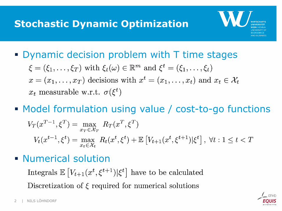
Stochastic Dynamic Optimization

§  Dynamic decision problem with T time stages

§  Model formulation using value / cost-to-go functions

§  Numerical solution

| NILS LÖHNDORF 2

From Trees to Lattices Scenario Generation for Stochastic Optimization

| NILS LÖHNDORF 3

5

50

40

40

30

40

30

30

20

40

30

30

20

30

20

20

10

45

35

35

25

35

25

25

15

40

30

30

20

35

25

30

55

45

35

25

15

5

50

40

30

20

10

45

35

25

15

40

30

20

35

25

30

Scenario Tree Scenario Lattice

State-time-history graph with 63 nodes and 32 scenarios

State-time graph with 21 nodes and 720 scenarios

Scenario Lattices A Compressed Scenario Representation

§  Lattices carry no information about the history of the process

§  Suitable for Markov processes where

§  Covers all state space type stochastic models: §  Autoregressive models §  Dynamic factor models §  Exponential smoothing §  Hidden Markov models §  Stochastic volatility models

| NILS LÖHNDORF 4

55

45

35

25

15

5

50

40

30

20

10

45

35

25

15

40

20

35

25

30

Scenario Lattice

30

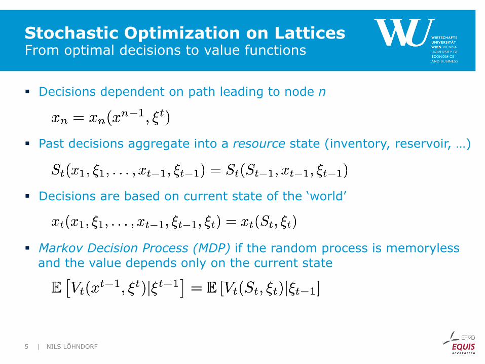
Stochastic Optimization on Lattices From optimal decisions to value functions

§  Decisions dependent on path leading to node n

§  Past decisions aggregate into a resource state (inventory, reservoir, …)

§  Decisions are based on current state of the ‘world’

§  Markov Decision Process (MDP) if the random process is memoryless and the value depends only on the current state

| NILS LÖHNDORF 5

Approximate Dual Dynamic Programming A solution strategy using scenario lattices

Each node of the lattice holds a value function

55

45

35

25

15

5

50

40

30

20

10

45

35

25

15

40

30

20

35

25

30

| NILS LÖHNDORF 6

V(S,ξ)

S

True Value Function

Hyperplane at S*

S*

Approximate the value function as minimum of a set of hyperplanes

1.  Construct a scenario lattice from a stochastic process

2.  Find an approximate value function for each node

How Do We Fit a Lattice From Data?

§  Parametric approach 1.  Estimate a Markovian time series process 2.  Reduce the continuous Markovian process to a lattice 3.  Determine an optimal policy using ADDP 4.  Evaluate the policy on the original time series model

§  Data-driven approach 1.  Estimate a lattice directly from data 2.  Determine an optimal policy using ADDP

Skip scenario reduction +

No policy validation needed

| NILS LÖHNDORF 7

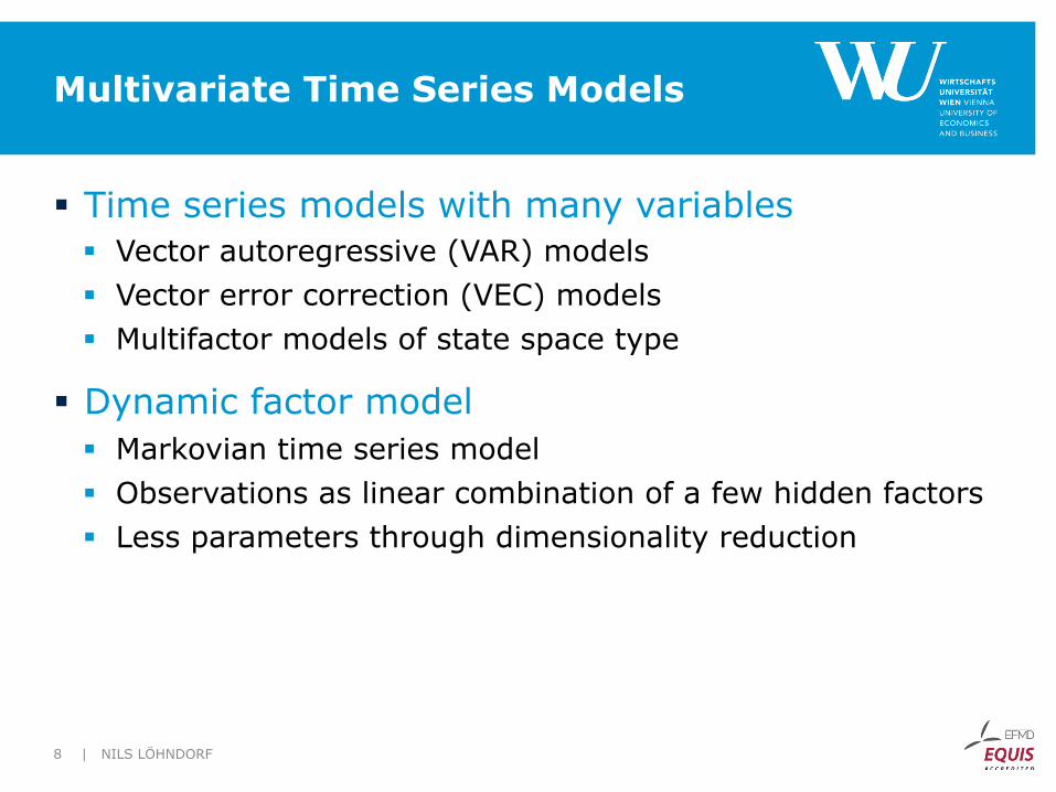
Multivariate Time Series Models

§  Time series models with many variables §  Vector autoregressive (VAR) models §  Vector error correction (VEC) models §  Multifactor models of state space type

§  Dynamic factor model §  Markovian time series model §  Observations as linear combination of a few hidden factors §  Less parameters through dimensionality reduction

| NILS LÖHNDORF 8

Dynamic Factor Model

t: time index Ft: vector of factors A: transition matrix Xt: vector of observations V: dynamic factor loadings B: parameter matrix of exogenous predictors Zt: exogenous predictors ut,vt: error term

| NILS LÖHNDORF 9

Ft = AFt�1 + ut

Xt = V Ft +BZt + vt

Dynamic Factor Lattice

§  Building blocks §  Represent factor space by set of discrete factors §  Replace linear state transition equation with

transition matrices

§  Learning a lattice from data 1.  Choose optimal quantizers of the data at stage t 2.  Count transitions between observations in the

neighborhood of quantizers at successive stages 3.  We use a moving time window of 30 days of observed

transitions to obtain a large enough sample

| NILS LÖHNDORF 10

Pt(F̄t|F̄t�1)

F̄

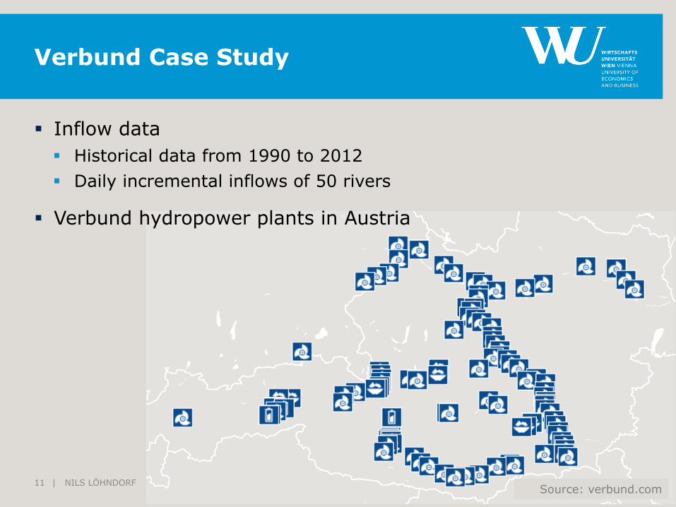
Source: verbund.com

Verbund Case Study

§  Inflow data §  Historical data from 1990 to 2012 §  Daily incremental inflows of 50 rivers

§  Verbund hydropower plants in Austria

| NILS LÖHNDORF 11

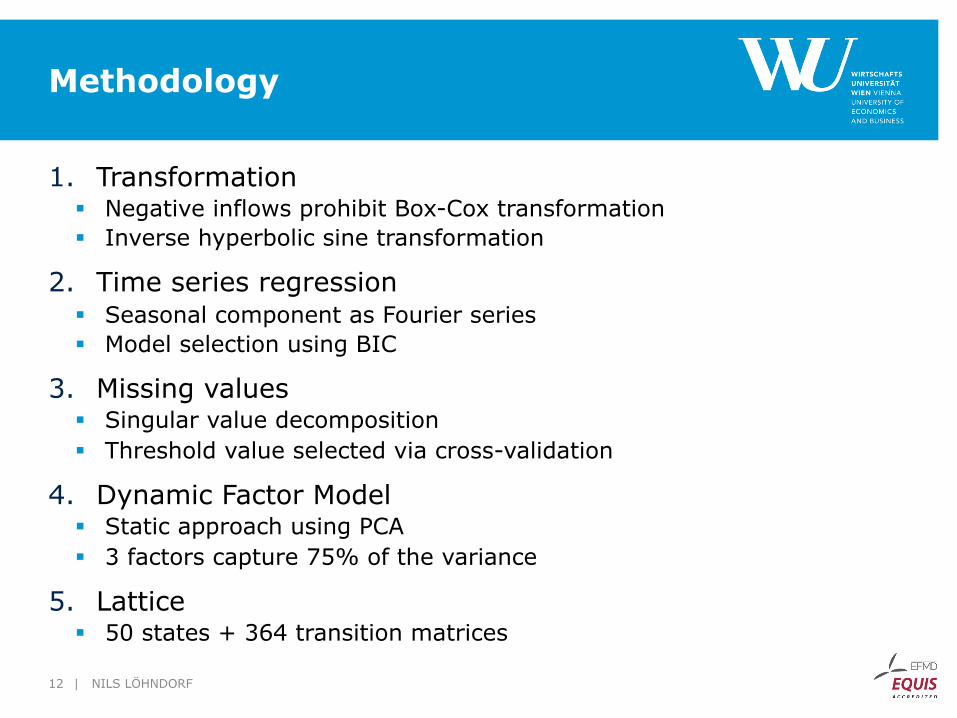
Methodology

1.  Transformation §  Negative inflows prohibit Box-Cox transformation §  Inverse hyperbolic sine transformation

2.  Time series regression §  Seasonal component as Fourier series §  Model selection using BIC

3.  Missing values §  Singular value decomposition §  Threshold value selected via cross-validation

4.  Dynamic Factor Model §  Static approach using PCA §  3 factors capture 75% of the variance

5.  Lattice §  50 states + 364 transition matrices

| NILS LÖHNDORF 12

Original vs Reduced Time Series

| NILS LÖHNDORF 13

Original vs Simulated Time Series

| NILS LÖHNDORF 14

Data à Factors à Lattice

Kernel Density Estimation

| NILS LÖHNDORF 16

Mean daily inflows

Mean annual inflows

– original data – lattice simulation

Conclusion

§  Results §  A small number of discrete states is sufficient to explain a

high-dimensional inflow process. §  Factors achieve longitudinal smoothing which helps to

extract long-range information

§  Outlook §  Semi-parametric extensions to overcome sparse state

transition samples

§  Future Work §  How do we measure the goodness of fit of a lattice?

| NILS LÖHNDORF 17

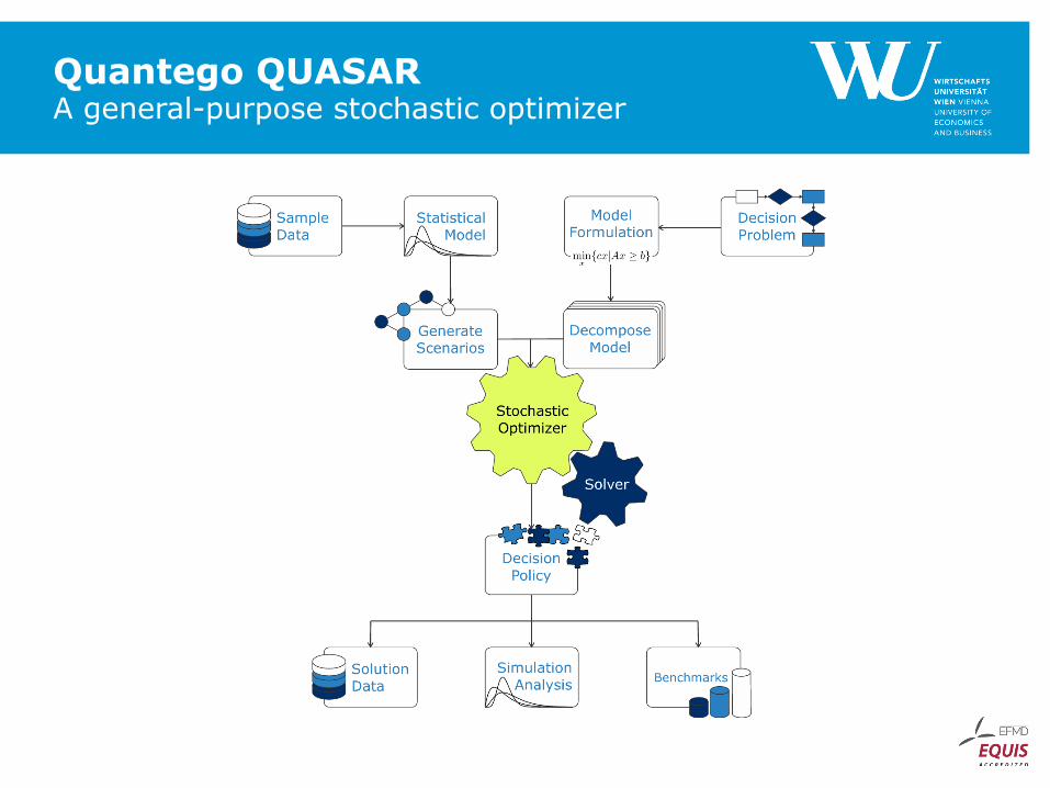
Quantego QUASAR A general-purpose stochastic optimizer