UPTEC F15053

Examensarbete 30 hpSeptember 2015

Modeling, control and state-estimation for an autonomous sailboat

Jon Melin

Teknisk- naturvetenskaplig fakultet UTH-enheten Besöksadress: Ångströmlaboratoriet Lägerhyddsvägen 1 Hus 4, Plan 0 Postadress: Box 536 751 21 Uppsala Telefon: 018 – 471 30 03 Telefax: 018 – 471 30 00 Hemsida: http://www.teknat.uu.se/student

Abstract

Modeling, control and state-estimation for anautonomous sailboat

Jon Melin

During long time missions with autonomous sailboats electrical power is a limitedresource. When making evaluations of power saving strategies it is important to havea good platform for simulations and experiments. In this thesis a model of a fourmeters long autonomous sailboat is presented and parameterized, several controlstrategies are developed and evaluated and state estimation algorithms for the windand the sailboat are developed, all with the purpose of future studies of powermanagement.

The model that is used captures the main characteristics of a sailboat quite well, it ispossible to use the model for controller development and state estimation. Themodel and the controllers are evaluated using simulations and experiments. Thecontrol strategy and state estimation algorithms shows promising results, but moreexperiments are needed to verify that simulations and the experiments are consistentin all conditions.

ISSN: 1401-5757, UPTEC F15053Examinator: Tomas NybergÄmnesgranskare: Thomas SchönHandledare: Matias Waller

Acknowledgements

First of all, I would like to express my gratitude to my supervisor at Aland Uni-versity of Applied Science Matias Waller, for your support during this project.I’m especially grateful for all the discussions we have had and I have always feltwelcome to come to you with my thoughts. Kjell Dahl also deserves a great thank,it has been pure enjoyment to work with you.

I would also like to thank Anna Friebe and Ronny Eriksson at Aland Universityof Applied Science for making it possible for me to take part in the project AlandSailing Robots and for inspiring discussions about autonomous sailing.

Thanks to my subject reviewer at Uppsala University, Thomas Schon for introduc-ing me to the beauty of control theory and the Aland Sailing Robots project.

Furthermore, all the members at the Aland Curling Club deserves a thank for allthe entertaining evenings at the rink.

Finally I would like to thank friends and family for their support and understand-ing.

iv

Contents

Acknowledgements iii

List of Figures vii

List of Tables viii

1 Introduction 11.1 Aland Sailing Robots . . . . . . . . . . . . . . . . . . . . . . . . . . 21.2 Microtransat challenge . . . . . . . . . . . . . . . . . . . . . . . . . 21.3 Motivation . . . . . . . . . . . . . . . . . . . . . . . . . . . . . . . . 31.4 Outline of thesis . . . . . . . . . . . . . . . . . . . . . . . . . . . . . 41.5 Associated publication . . . . . . . . . . . . . . . . . . . . . . . . . 41.6 System description . . . . . . . . . . . . . . . . . . . . . . . . . . . 5

1.6.1 Hardware . . . . . . . . . . . . . . . . . . . . . . . . . . . . 51.6.2 Software . . . . . . . . . . . . . . . . . . . . . . . . . . . . . 7

2 Modeling 92.1 Reference systems, states and variables . . . . . . . . . . . . . . . . 102.2 Model equations . . . . . . . . . . . . . . . . . . . . . . . . . . . . . 102.3 True and apparent wind . . . . . . . . . . . . . . . . . . . . . . . . 112.4 Acting forces . . . . . . . . . . . . . . . . . . . . . . . . . . . . . . 13

2.4.1 Sail force . . . . . . . . . . . . . . . . . . . . . . . . . . . . . 132.4.2 Rudder force . . . . . . . . . . . . . . . . . . . . . . . . . . 142.4.3 Friction . . . . . . . . . . . . . . . . . . . . . . . . . . . . . 14

2.5 Model simulations . . . . . . . . . . . . . . . . . . . . . . . . . . . . 142.6 Experiments . . . . . . . . . . . . . . . . . . . . . . . . . . . . . . . 15

2.6.1 GPS coordinates and great circles . . . . . . . . . . . . . . . 162.7 Comparison of simulation and experiment . . . . . . . . . . . . . . 17

3 Control 213.1 Control strategy . . . . . . . . . . . . . . . . . . . . . . . . . . . . . 22

v

vi Contents

3.1.1 Rudder control . . . . . . . . . . . . . . . . . . . . . . . . . 233.2 Rudder control evaluation . . . . . . . . . . . . . . . . . . . . . . . 24

4 State estimation 294.1 Sailboat filter . . . . . . . . . . . . . . . . . . . . . . . . . . . . . . 30

4.1.1 Discretization of model equations . . . . . . . . . . . . . . . 304.1.2 Measurement equations . . . . . . . . . . . . . . . . . . . . . 314.1.3 Extended Kalman filter equations . . . . . . . . . . . . . . . 31

4.2 Wind filter . . . . . . . . . . . . . . . . . . . . . . . . . . . . . . . . 324.3 Filter implementation and results . . . . . . . . . . . . . . . . . . . 33

5 Concluding remarks 375.1 Conclusions and discussion . . . . . . . . . . . . . . . . . . . . . . . 375.2 Further work . . . . . . . . . . . . . . . . . . . . . . . . . . . . . . 39

Bibliography 40

List of Figures

1.1 The sailboat and parts of the team . . . . . . . . . . . . . . . . . . 11.2 Experimental system overview . . . . . . . . . . . . . . . . . . . . . 51.3 Electronic system . . . . . . . . . . . . . . . . . . . . . . . . . . . . 61.4 Remote radio control . . . . . . . . . . . . . . . . . . . . . . . . . . 71.5 Raspberry Pi 2 Model B v1.1 . . . . . . . . . . . . . . . . . . . . . 71.6 XBee module . . . . . . . . . . . . . . . . . . . . . . . . . . . . . . 71.7 Wind sensor . . . . . . . . . . . . . . . . . . . . . . . . . . . . . . . 7

2.1 Degrees of freedom of ships . . . . . . . . . . . . . . . . . . . . . . 102.2 Explanation of the states in the model . . . . . . . . . . . . . . . . 112.3 Definition of wind . . . . . . . . . . . . . . . . . . . . . . . . . . . . 122.4 Trajectory. Test case Circle . . . . . . . . . . . . . . . . . . . . . . 182.5 Speed profile. Test case Circle . . . . . . . . . . . . . . . . . . . . . 182.6 Trajectory. Test case Straight line . . . . . . . . . . . . . . . . . . . 192.7 Speed profile. Test case Straight line . . . . . . . . . . . . . . . . . 192.8 Trajectory. Test case Tack . . . . . . . . . . . . . . . . . . . . . . . 192.9 Speed profile. Test case Tack . . . . . . . . . . . . . . . . . . . . . 19

3.1 Comparison of rudder angle as a function control error . . . . . . . 253.2 Rudder comparison simulation . . . . . . . . . . . . . . . . . . . . . 263.3 Comparison of rudder angle as a function control error . . . . . . . 273.4 Trajectory from experiment with controller . . . . . . . . . . . . . . 28

4.1 True wind direction . . . . . . . . . . . . . . . . . . . . . . . . . . . 344.2 True wind speed . . . . . . . . . . . . . . . . . . . . . . . . . . . . . 344.3 Trajectory from state estimation, p4 = 200kg s−1 . . . . . . . . . . . 354.4 Trajectory from state estimation, p4 = 500kg s−1 . . . . . . . . . . . 35

vii

List of Tables

2.1 Model parameters . . . . . . . . . . . . . . . . . . . . . . . . . . . . 122.2 Model parameters and their values . . . . . . . . . . . . . . . . . . 20

3.1 Parameters used in the controller . . . . . . . . . . . . . . . . . . . 233.2 Performance evaluation of rudder control . . . . . . . . . . . . . . . 25

viii

Chapter 1

Introduction

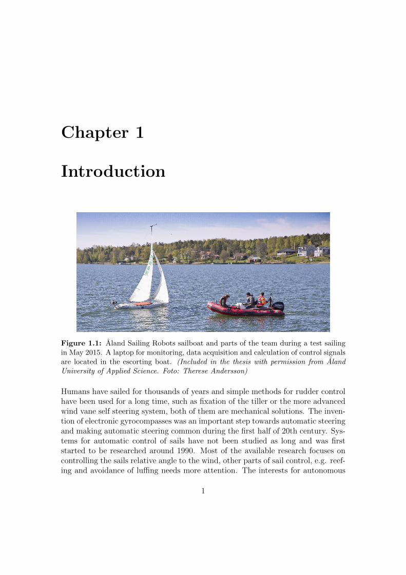
Figure 1.1: Aland Sailing Robots sailboat and parts of the team during a test sailingin May 2015. A laptop for monitoring, data acquisition and calculation of control signalsare located in the escorting boat. (Included in the thesis with permission from AlandUniversity of Applied Science. Foto: Therese Andersson)

Humans have sailed for thousands of years and simple methods for rudder controlhave been used for a long time, such as fixation of the tiller or the more advancedwind vane self steering system, both of them are mechanical solutions. The inven-tion of electronic gyrocompasses was an important step towards automatic steeringand making automatic steering common during the first half of 20th century. Sys-tems for automatic control of sails have not been studied as long and was firststarted to be researched around 1990. Most of the available research focuses oncontrolling the sails relative angle to the wind, other parts of sail control, e.g. reef-ing and avoidance of luffing needs more attention. The interests for autonomous

1

2 1.1. Aland Sailing Robots

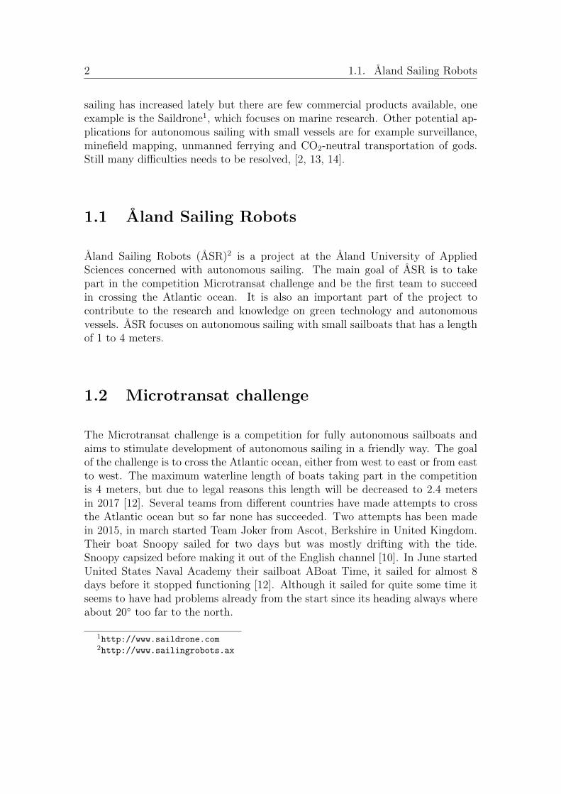
sailing has increased lately but there are few commercial products available, oneexample is the Saildrone1, which focuses on marine research. Other potential ap-plications for autonomous sailing with small vessels are for example surveillance,minefield mapping, unmanned ferrying and CO2-neutral transportation of gods.Still many difficulties needs to be resolved, [2, 13, 14].

1.1 Aland Sailing Robots

Aland Sailing Robots (ASR)2 is a project at the Aland University of AppliedSciences concerned with autonomous sailing. The main goal of ASR is to takepart in the competition Microtransat challenge and be the first team to succeedin crossing the Atlantic ocean. It is also an important part of the project tocontribute to the research and knowledge on green technology and autonomousvessels. ASR focuses on autonomous sailing with small sailboats that has a lengthof 1 to 4 meters.

1.2 Microtransat challenge

The Microtransat challenge is a competition for fully autonomous sailboats andaims to stimulate development of autonomous sailing in a friendly way. The goalof the challenge is to cross the Atlantic ocean, either from west to east or from eastto west. The maximum waterline length of boats taking part in the competitionis 4 meters, but due to legal reasons this length will be decreased to 2.4 metersin 2017 [12]. Several teams from different countries have made attempts to crossthe Atlantic ocean but so far none has succeeded. Two attempts has been madein 2015, in march started Team Joker from Ascot, Berkshire in United Kingdom.Their boat Snoopy sailed for two days but was mostly drifting with the tide.Snoopy capsized before making it out of the English channel [10]. In June startedUnited States Naval Academy their sailboat ABoat Time, it sailed for almost 8days before it stopped functioning [12]. Although it sailed for quite some time itseems to have had problems already from the start since its heading always whereabout 20◦ too far to the north.

1http://www.saildrone.com2http://www.sailingrobots.ax

Chapter 1. Introduction 3

1.3 Motivation

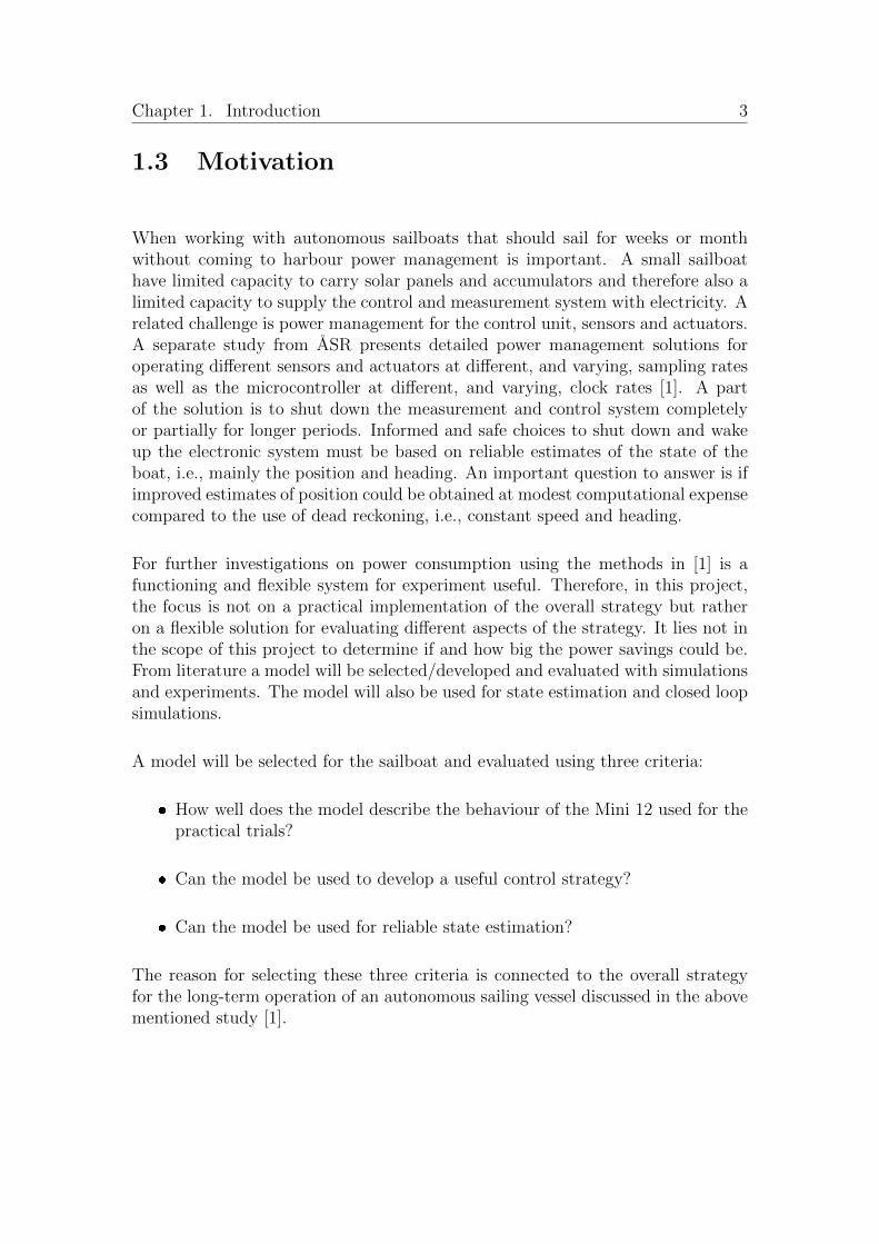
When working with autonomous sailboats that should sail for weeks or monthwithout coming to harbour power management is important. A small sailboathave limited capacity to carry solar panels and accumulators and therefore also alimited capacity to supply the control and measurement system with electricity. Arelated challenge is power management for the control unit, sensors and actuators.A separate study from ASR presents detailed power management solutions foroperating different sensors and actuators at different, and varying, sampling ratesas well as the microcontroller at different, and varying, clock rates [1]. A partof the solution is to shut down the measurement and control system completelyor partially for longer periods. Informed and safe choices to shut down and wakeup the electronic system must be based on reliable estimates of the state of theboat, i.e., mainly the position and heading. An important question to answer is ifimproved estimates of position could be obtained at modest computational expensecompared to the use of dead reckoning, i.e., constant speed and heading.

For further investigations on power consumption using the methods in [1] is afunctioning and flexible system for experiment useful. Therefore, in this project,the focus is not on a practical implementation of the overall strategy but ratheron a flexible solution for evaluating different aspects of the strategy. It lies not inthe scope of this project to determine if and how big the power savings could be.From literature a model will be selected/developed and evaluated with simulationsand experiments. The model will also be used for state estimation and closed loopsimulations.

A model will be selected for the sailboat and evaluated using three criteria:

� How well does the model describe the behaviour of the Mini 12 used for thepractical trials?

� Can the model be used to develop a useful control strategy?

� Can the model be used for reliable state estimation?

The reason for selecting these three criteria is connected to the overall strategyfor the long-term operation of an autonomous sailing vessel discussed in the abovementioned study [1].

4 1.4. Outline of thesis

1.4 Outline of thesis

In section 1.6, the sailboat used in this project is described, including the boatitself, the electronics and the software. In chapter 2 a sailboat model is pre-sented, parametrized and evaluated. This chapter also includes a description ofhow simulations and experiments were performed. In chapter 3 a control strategyis presented and evaluated. Chapter 4 includes the theory necessary for imple-menting the filters used for state-estimation and some results indicating what thefilters might be capable of. Chapter 5 includes conclusions and a discussion aboutthe results presented in the previous chapters together with recommendations forfurther work.

1.5 Associated publication

In addition to this report the work performed in this thesis did also result in apaper, Modeling and control for an autonomous sailboat: A case study, acceptedfor publication and presentation at the 8th International Robotic Sailing Confer-ence in Mariehamn, Aland Islands, August 2015 [11]. The paper was written incooperation with Kjell Dahl and Matias Waller. Some formulations in this reportis taken directly from the paper.

Chapter 1. Introduction 5

1.6 System description

The sailboat used for the experiments in this project is shown in figure 1.1, it hasan overall length of just over 4 meters. The sailboat is of the model Mini-12 andalso qualifies to the 2.4mR-class of the International Sailing Federation. It weighsabout 300 kg. The maximum angle the rudder can make with the keel is 30◦ andthe maximum angle the main sail can make is about 35◦, this limitation is dueto the way the actuator controlling the main sheet is installed. Meaning that theactual maximum sail angle is larger.

Although a primary goal of the project is to have an autonomous and energy-efficient measurement and control system, the experimental setup used in thisproject is designed for easy supervision and real-time evaluation. To achieve thisit is necessary to have a way of transferring information, in real time, from thesensors on board the boat to a laptop in a nearby boat. Therefore a wireless linkwas installed during this project. The other hardware, presented next, was alreadyinstalled prior to this project.

Figure 1.2: Experimental system overview, the on-board system to the left communi-cating wireless with a laptop.

1.6.1 Hardware

The hardware setup used during this project, figure 1.2, mainly uses the systemon board the sailboat for reading sensors and writing signals to the actuators.Calculations of control signals to the actuators as well as presentation of sensorreadings is done on the laptop.

A diagram of the electronic system on board the sailboat is provided in figure 1.3.The main unit in the system is a Raspberry Pi (2 model B v1.1), a small sin-gle board computer, figure 1.5. The Raspberry Pi collects data from all sensors

6 1.6. System description

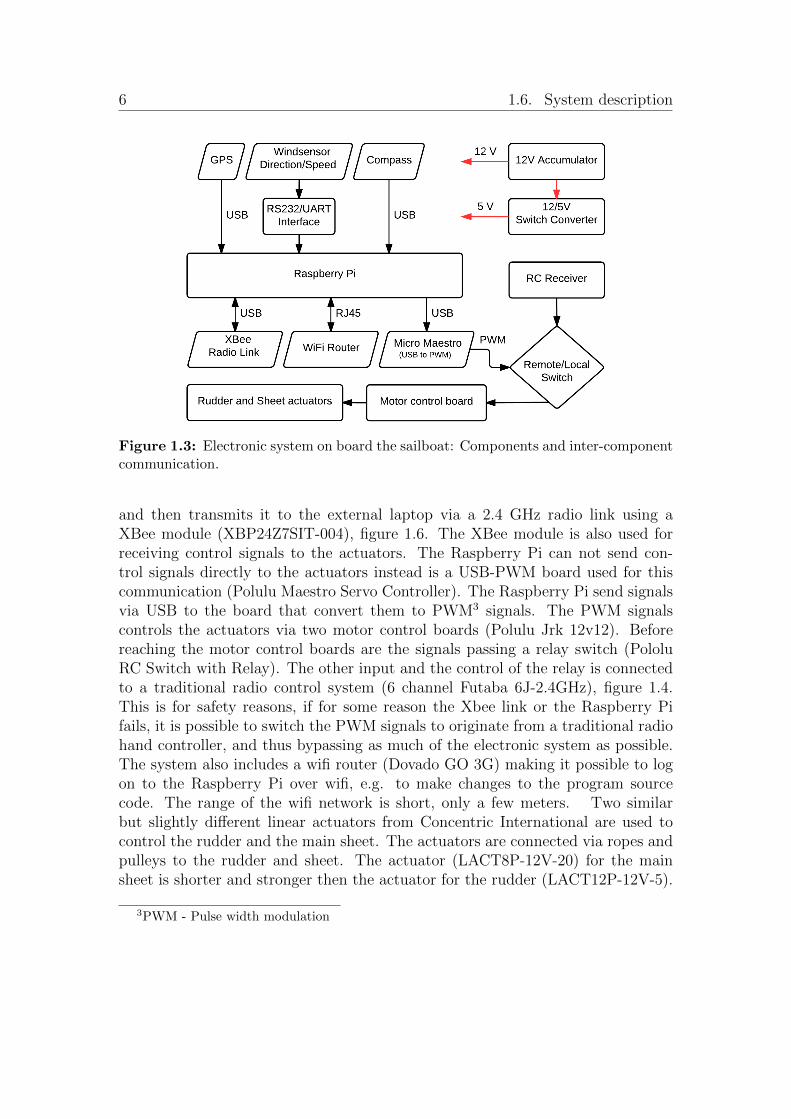
Figure 1.3: Electronic system on board the sailboat: Components and inter-componentcommunication.

and then transmits it to the external laptop via a 2.4 GHz radio link using aXBee module (XBP24Z7SIT-004), figure 1.6. The XBee module is also used forreceiving control signals to the actuators. The Raspberry Pi can not send con-trol signals directly to the actuators instead is a USB-PWM board used for thiscommunication (Polulu Maestro Servo Controller). The Raspberry Pi send signalsvia USB to the board that convert them to PWM3 signals. The PWM signalscontrols the actuators via two motor control boards (Polulu Jrk 12v12). Beforereaching the motor control boards are the signals passing a relay switch (PololuRC Switch with Relay). The other input and the control of the relay is connectedto a traditional radio control system (6 channel Futaba 6J-2.4GHz), figure 1.4.This is for safety reasons, if for some reason the Xbee link or the Raspberry Pifails, it is possible to switch the PWM signals to originate from a traditional radiohand controller, and thus bypassing as much of the electronic system as possible.The system also includes a wifi router (Dovado GO 3G) making it possible to logon to the Raspberry Pi over wifi, e.g. to make changes to the program sourcecode. The range of the wifi network is short, only a few meters. Two similarbut slightly different linear actuators from Concentric International are used tocontrol the rudder and the main sheet. The actuators are connected via ropes andpulleys to the rudder and sheet. The actuator (LACT8P-12V-20) for the mainsheet is shorter and stronger then the actuator for the rudder (LACT12P-12V-5).

3PWM - Pulse width modulation

Chapter 1. Introduction 7

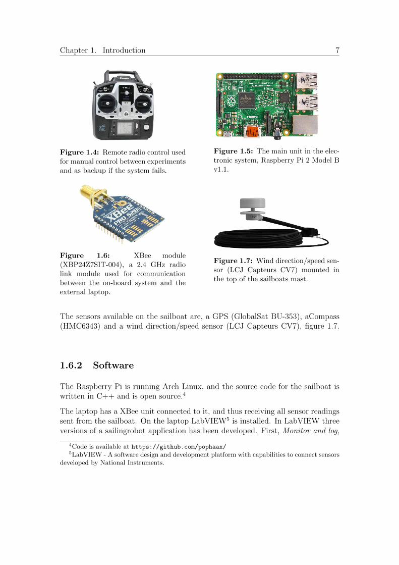
Figure 1.4: Remote radio control usedfor manual control between experimentsand as backup if the system fails.

Figure 1.5: The main unit in the elec-tronic system, Raspberry Pi 2 Model Bv1.1.

Figure 1.6: XBee module(XBP24Z7SIT-004), a 2.4 GHz radiolink module used for communicationbetween the on-board system and theexternal laptop.

Figure 1.7: Wind direction/speed sen-sor (LCJ Capteurs CV7) mounted inthe top of the sailboats mast.

The sensors available on the sailboat are, a GPS (GlobalSat BU-353), aCompass(HMC6343) and a wind direction/speed sensor (LCJ Capteurs CV7), figure 1.7.

1.6.2 Software

The Raspberry Pi is running Arch Linux, and the source code for the sailboat iswritten in C++ and is open source.4

The laptop has a XBee unit connected to it, and thus receiving all sensor readingssent from the sailboat. On the laptop LabVIEW5 is installed. In LabVIEW threeversions of a sailingrobot application has been developed. First, Monitor and log,

4Code is available at https://github.com/pophaax/5LabVIEW - A software design and development platform with capabilities to connect sensors

developed by National Instruments.

8 1.6. System description

which is presenting all sensor readings in a GUI and storing every received messagein a text file. The second version Manual control, does the same thing and alsoenables the possibility to send control signals given by the user to the sailboatsactuators. This means that both the control signals sent and the control signalsused at every time instance will be logged. Due to communication delays, these twosignals differ slightly. The third version Controller is the most complex version,its main purpose is to implement a controller by letting the laptop calculate thecontrol signals. This version is made in such a way that it is possible for theuser to easy and in real time switch between and manual and automatic controlof rudder and main sheet separately. It also includes the possibility choose howand if the wind should be filtered. The parts of the application that filters thewind and calculates the control signals is implemented with a MATLAB6-scriptblock, enabling the use of the same MATLAB functions written for simulations,thus is the risk of implementation errors of these steps in the applications verysmall. It is possible for the user to turn of the filter and manually set values forwind directions and speed. Altogether this makes the application a good tool fortesting new controllers that has been developed and simulated in MATLAB.

6MATLAB - numerical computing environment developed by MathWorks

Chapter 2

Modeling

For the purpose of navigation and control of ships, a rather exhaustive presentationof models can be found in the book by Fossen [3]. The book is mainly about shipsand underwater vehicles, but a similar approach to modelling has been extendedto sailboats in [15]. The model presented in [15] has also been used as a basis fortheoretical studies on simulations of, and control strategies for sailboats [6, 9]. Asimplified model has been presented in [8], with a modest number of parametersand thus an attractive alternative for control design and state estimation. Giventhe success of practical trials for autonomous tracking by a sailboat achieved bythe team around Jaulin, it seems that the simple model captures the dynamics ofa sailboat essential for controller design. Therefore, the model presented in [8] isalso chosen as the basis for the model development of the present project.

It is necessary to make some initial assumptions in order to keep the model sim-ple.

� Motion is confined to a horizontal plane at see level without roll or pitch.This gives a model with 3 degrees of freedom: surge, sway and yaw definedin figure 2.1.

� Influence from waves and currents will be neglected.

� Velocity is assumed to be small, therefore Coriolis and Centripetal forces areneglected. Also the damping coefficients could be assumed to be linear ofthe same reason.

� The mainsail and the foresail is combined into one effective sail

9

10 2.1. Reference systems, states and variables

Figure 2.1: Movement of ships is often refereed to as surge, sway, heave, roll, pitchand yaw, e.g. 6 degrees of freedom.

2.1 Reference systems, states and variables

In order to represent all states of the sailboat and measurements, several refer-ence systems are needed. The sailboats position, x, y, heading, θ, and rotationalspeed, ω, is given in a North-East-Up reference frame (n-frame), i.e. an easterlyx-axis and northerly y-axis, figure 2.2. The n-frame is earth fixed and assumedto be inertial for local navigation and its origin in simulations and experimentswill be set to the sailboats starting point, e.g. the n-frame is a tangential plane tothe surface of the earth. For the experiments in this project is this approximationsufficient, but when sailing over longer distances, such as the Atlantic ocean, thecurvature of the earth must be taken into consideration.

It is also necessary to define a sailboat fixed reference frame (b-frame). The originof the b-frame lies in the boats center of gravity (CoG) which also is assumed tocoincide with the boats center of rotation (CoR), figure 2.2. In the b-frame is the

sailboats speed, v, distances on the sailboat and the control signals u =[δr δs

]Tdefined. δr is the angle of the rudder and δs is the angle of the sail which isproportional to the length of the mainsheet.

2.2 Model equations

The model is based on traditional translational and rotational inertia affected byforces, yielding changes in position, orientation, speed and rotation. In equation(2.2) the model is given by non-linear differential equations in state space with

five states, x =[x y θ v ω

]T, defined in section 2.1. Drift and change in position

Chapter 2. Modeling 11

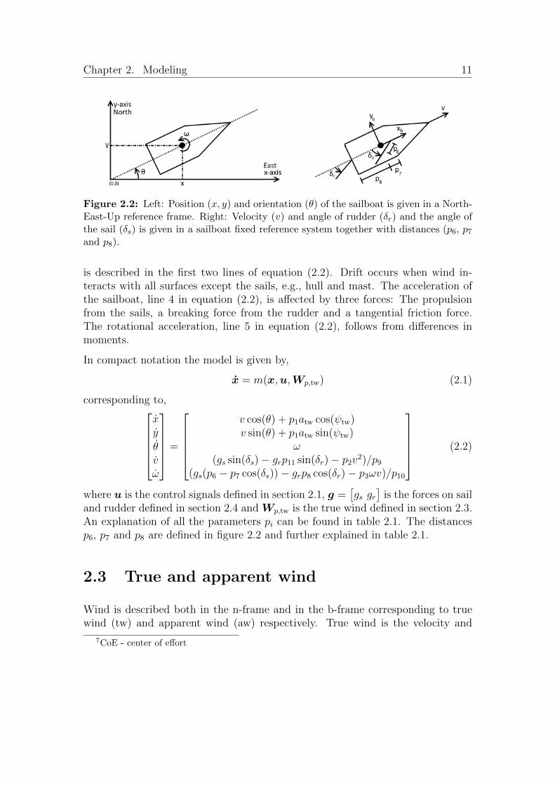
Figure 2.2: Left: Position (x, y) and orientation (θ) of the sailboat is given in a North-East-Up reference frame. Right: Velocity (v) and angle of rudder (δr) and the angle ofthe sail (δs) is given in a sailboat fixed reference system together with distances (p6, p7and p8).

is described in the first two lines of equation (2.2). Drift occurs when wind in-teracts with all surfaces except the sails, e.g., hull and mast. The acceleration ofthe sailboat, line 4 in equation (2.2), is affected by three forces: The propulsionfrom the sails, a breaking force from the rudder and a tangential friction force.The rotational acceleration, line 5 in equation (2.2), follows from differences inmoments.

In compact notation the model is given by,

x = m(x,u,Wp,tw) (2.1)

corresponding to,xy

θvω

=

v cos(θ) + p1atw cos(ψtw)v sin(θ) + p1atw sin(ψtw)

ω(gs sin(δs)− grp11 sin(δr)− p2v2)/p9

(gs(p6 − p7 cos(δs))− grp8 cos(δr)− p3ωv)/p10

(2.2)

where u is the control signals defined in section 2.1, g =[gs gr

]is the forces on sail

and rudder defined in section 2.4 and Wp,tw is the true wind defined in section 2.3.An explanation of all the parameters pi can be found in table 2.1. The distancesp6, p7 and p8 are defined in figure 2.2 and further explained in table 2.1.

2.3 True and apparent wind

Wind is described both in the n-frame and in the b-frame corresponding to truewind (tw) and apparent wind (aw) respectively. True wind is the velocity and

7CoE - center of effort

12 2.3. True and apparent wind

Table 2.1: Model parameters

p1 - drift coefficient p7 [m] distance to mastp2 [kgs−1] tangential friction p8 [m] distance to rudderp3 [kgm] angular friction p9 [kg] mass of boatp4 [kgs−1] sail lift p10 [kgm2] moment of inertiap5 [kgs−1] rudder lift p11 - rudder break coefficientp6 [m] distance to sail CoE7

Figure 2.3: Definition of true wind, wind relative an earth fixed point, and apparentwind, wind relative the sailboat.

direction of the air measured from a platform fixed to the ground, e.g. the wind asit is experienced by a person standing still on a pier. Apparent wind is the velocityand direction of the wind measured from a moving object, e.g. the wind as it isexperienced by a person standing at the fore of a ship. Figure 2.3 illustratesthe angle ψ and speed a of the wind in polar coordinates in both frames. For

convenience Wp,tw =[atw ψtw

]Tis introduced. Given the speed and heading of the

boat, true wind can be calculated from the apparent wind or vice versa. Apparentwind in Cartesian coordinates relative to the direction of the boat, i.e., the firstcoordinate corresponding to the heading of the boat can be calculated from truewind by

Wc,aw =

[atw cos(ψtw − θ)− vatw sin(ψtw − θ)

](2.3)

The corresponding polar coordinates are thus given by

Wp,aw =

[aawψaw

]=

[|Wc,aw|

atan2(Wc,aw)

](2.4)

where atan2 is the arctangens function with two arguments returning an angle inthe correct quadrant.

Chapter 2. Modeling 13

2.4 Acting forces

It is possible to apply basic aerohydrodynamic theory if sail and rudder are re-garded as thin foils. This means that the forces acting on the sail and rudder dueto the medium flowing around them could be simplified into a lift and a drag forceacting in a center of effort, equation (2.5). The drag force is acting co-linear tothe apparent wind and lift force is acting perpendicular.

L =1

2ρAv2aCL

D =1

2ρAv2aCD

(2.5)

where ρ is the density of flowing medium, A is the plane area of the foil, va isthe mediums apparent velocity, CL and CD are lift and drag coefficients respec-tively. These coefficients depends on the mediums angle of attack, α and the foilsshape.

In [15] it can be seen that the drag and lift coefficients could be approximatedby,

CL = k1 sin(2α)

CD = k1(1− cos(2α))(2.6)

where k1 is a constant. This means that the lift and drag forces can be combinedinto one force, g, acting perpendicular to the sail/rudder.

g = L cos(α) +D sin(α) =

= k1

2v2a(sin(2α) cos(α) + (1− cos(2α)) sin(α)) =

= kv2a sin(α)

(2.7)

where k = k1ρA.

2.4.1 Sail force

The angle of attack, αs, on the sail is determined by the direction of the apparentwind and the angle of the sail, αs = ψaw− δs, where the apparent wind is given byequation (2.4). The force on the sail is thus given by,

gs = −p4aaw sin(δs − ψaw) (2.8)

where p4 is the lift coefficient of the sail. When the velocity of the apparent windincrease, the roll angle of the boat will increase resulting in a smaller effective area

14 2.5. Model simulations

of sail. This is in parts accounted for by skipping the square on the apparent windspeed. The sheet is flexible and therefore the sail cannot hold against the windand thus stall the boat. This is accounted for by letting the model update theangle of the sail with equation (2.9).

δs = −sgn(ψaw)) min(|π − |ψaw||, |δs|) (2.9)

where |ψaw| ≤ π and sgn is the sign function.

2.4.2 Rudder force

The apparent velocity of the water near the rudder is assumed to be parallel tothe boats heading, e.g. no currents or vortexes produced by the hull affects therudder. The angle of attack then becomes, αr = −δr, and the magnitude of theapparent velocity becomes equal to the boats velocity. The force on the rudder isthus given by,

gr = −p5v2 sin(δr) (2.10)

where p5 is the lift coefficient of the rudder.

To make the model in equation (2.1) easier to read the sail and rudder forces isredefined by moving the minus signs from equation (2.10) and (2.8) into (2.1). Insummary, the sail and rudder force is given by,

g =

[gsgr

]=

[p4aaw sin(δs − ψaw)

p5v2 sin(δr)

](2.11)

2.4.3 Friction

The boat is affected by some frictional forces, first a tangential friction force act-ing in the opposite direction of the sailboats heading. This force is assumed tobe proportional to the square of the sailboats speed, p2v

2. The model also in-cludes a rotational friction force proportional to the sailboats speed and rotationalspeed, p3ωv. The frictional forces could also be seen as damping elements in themodel.

2.5 Model simulations

For simulations of the model, presentation of recorded data and comparisons ofsimulations and experiments the software MATLAB is used. The model is imple-mented in a m-file and could be called at as a function. When the model function

Chapter 2. Modeling 15

is given the current state of the sailboat, true wind and control signals for rudderand sail, the derivative of each sailboat state is returned. The function includes allof the equations presented in the chapter so far and the values of the model param-eters from table 2.2. For simulations are the differential equations in the modelsolved with MATLAB’s differential equation solver ode45. The solver is given ahandle to the model function and a time interval to solve for, in this interval thewind and the control signals are assumed to be constant. Between each intervalthe values of the wind and control signals could be updated. For most simulationsis the interval length set to 1 s, resulting in a controller running at 1 Hz.

The controllers and filters in chapter 3 and 4 are also implemented as functionswith the function calls stated on the form in listing 2.1. With this structure it iseasy to compare different parts, e.g. different controllers or filters, by making smallchanges in the main file. Also, as stated in section 1.6.2, blocks with MATLABcode could be created in the LabVIEW program used for collecting data, and thuslimiting the risk of implementation errors when porting code from simulations tothe platform used for experiments.

Listing 2.1: Functions calls in MATLAB for code written in this project.

function dstate dt = model(t,state,W,u)function [delta r, delta s] = controller X(state, W, param)function [xhat out, P out] = filter X(T,measurments,Q,R)

2.6 Experiments

The goal of the first experiments was to collect data for model parametrizationand for filtering. Later, experiments for testing a controller were performed. Inorder to collect good data for the model parametrization some test cases werechosen. Similar cases could be found in [3], where they are used in tuning andevaluation processes of ship autopilots.

� Circle The sailboat sails in circles by setting constant rudder angle and sheetlength. This tests the sailboats ability to handle wind from all directions andits acceleration when the wind starts to fill the sails.

� Straight line The sailboat sails with wind coming from the side, neutralrudder and constant sheet length. This case tests the balance between theforces generated by the sails and friction, together with the size of the drift.

� Tacking The sailboat tacks, that is sails on alternating sides of the wind

16 2.6. Experiments

and therefore advances towards the wind. This is the most complex case,testing the interaction between all parts of the model, especially rudder andsail forces.

In the experiments data from all sensors is sent to a laptop over the wireless link,and in real time presented to the user and stored for later analysis. The controlsignals to the actuators is decided by the user on the laptop and sent to the sailboatover the wireless link and also saved in the data files. Due to the design of thesoftware on the laptop and on board the sailboat a delay of 1-3 seconds in thecontrol signals is experienced. In this delay, also some of the time it takes tomove the actuator is included, the rudder could be adjusted with about 16◦/s.Meaning that the rudder needs about 2 seconds to go from neutral to its maximalangle.

It is the relation between the force parameters (p2, p3, p4 and p5) and the mass/in-ertia that are important rather than values of the parameters them self. Theparametrization is done by first estimating the sailboats mass, p9 = 300 kg, andits moment of inertia. The moment of inertia is calculated with the correspondingequation for a rectangular plate with length l and width w,

p10 = p9l2 + w2

12= 400 kg m2 (2.12)

where l = 4m and w = 1m. The distance parameters (p6, p7 and p8) is estimatedfrom their physical interpretation on the boat. Since the boat has two sails andthe model only has one it is impossible to measure the parameters directly.

All other model parameters, that could not be estimated by logical reasoning,were chosen in an iterative way by changing parameter values and comparing thetrajectory of simulations and experiments. In the simulations measurements fromcorresponding experiment of wind, rudder angle and sail angle are used as inputto the model. As a start parameters from [8] was chosen. Both the result fromthe parametrization and the values in [8] could be found in table 2.2.

2.6.1 GPS coordinates and great circles

The GPS unit gives the current position in decimal degrees relative the equatorand the prime meridian. In the model it is assumed that the sailboat is movingin a plane, not an a sphere, and position is given as distances to the origin alongthe x- and y-axis, e.g. a local navigation frame is used. And also, the positionoutput from simulations are given in meters relative the origin. In order to make

Chapter 2. Modeling 17

it possible to compare simulations and experiments it is necessary to map GPScoordinates to rectangular coordinates in the local navigation frame.

Since all experiments is conducted in the western harbour of Mariehamn, 60.1074◦

and 19.9218◦ was chosen as the latitude and longitude of the origin, e.g. thecenter of the local navigation frame. If both the coordinate of the origin and thepresent position is expressed in radians the distance from the origin is given bythe spherical law of cosine,

∆σx = arccos(sin(φo) sin(φo) + cos(φo) cos(φo) cos(|λo − λp|))∆σy = arccos(sin(φo) sin(φp) + cos(φo) cos(φp) cos(|λo − λo|))sx = r∆σx sgn(λp − λo)sy = r∆σy sgn(φp − φo)

(2.13)

where φo, λo and φp, λp are the latitude and longitude of the origin and theposition, sgn is the sign function and r is the radius of the earth8. The position inmeters relative the origin is now given by

[sx sy

].

2.7 Comparison of simulation and experiment

In figures 2.4–2.9 the trajectories and speed profiles from simulations and exper-iments described in section 2.6 are found. The blue arrow in the middle of thetrajectory figures indicates the mean wind direction during each experiment. The,by the sailboat measured, mean true wind speed during each experiment was: 2.9,3.5, 5.0 m/s for respective case. Figure 2.8 shows tacking manoeuvres, the ruddercontrol signal from the experiment in this simulation is slightly modified. A glitchof ±3◦ is applied, within the glitch is δr set to zero. This removes small rudderactivity that didn’t affected the sailboat, but affected the model. It should benoted that the rudder actuator is connected to the rudder with ropes that hassome elasticity. That is a likely explanation to why the sailboat didn’t react tothe small rudder adjustments made during this experiment.

In figure 2.4 and 2.5 it is seen that the simulated speed corresponds quite wellto the measured speed but a bigger difference is noted in the trajectories. Inthe experiment the sailboat sailed a little bit straighter for a while, lower leftcorner in figure 2.4. The reason for this straighter trajectory is not clear, but itcould explain parts of the difference of the trajectory and why the sailboat in thesimulation turns to early.

8Earth radius, r = 6371 km

18 2.7. Comparison of simulation and experiment

Figure 2.4: Test case Circle. GPS po-sition from experiment and simulatedtrajectory using constant rudder result-ing in circles.

Figure 2.5: Test case Circle. Mea-sured speed over ground from GPSin experiment and simulated speed asfunction of time.

In figure 2.6 and 2.7 the trajectory and speed profile of simulation and experimentare consistent.

In figure 2.8 and 2.9 again some differences in trajectories are seen. This test iscomplex and it is hard to simulate the correct heading after a couple of tacks. Theintegrated error in heading will rapidly be so large that no relevant comparisoncould be made if the parametrization of the model is bad.

The parametrization of the model is done on basis of the data in above mentionedfigures. The parameter values chosen, used in all of the presented simulations, ispresented in table 2.2. Most parameters have similar values as the original onesin [8], but some differences exists even though the two sailboats are of similarsize, same weight. For example, the tangential friction is larger and the sail lift issmaller. A possible explanation could be that the sailboats has different rigs, thesailboat in [8] has a balanced rig instead of a sloop rig. Other noticeable differencesis the moment of inertia and the rudder break coefficient, were the later doesn’texist in [8].

Chapter 2. Modeling 19

Figure 2.6: Test case Straight line.GPS position from experiment and sim-ulated trajectory using neutral rudderresulting in a straight line.

Figure 2.7: Test case Straight line.Measured speed over ground from GPSin experiment and simulated speed asfunction of time.

Figure 2.8: Test case Tack. GPS posi-tion from experiment and simulated tra-jectory.

Figure 2.9: Test case Tack. Measuredspeed over ground from GPS in exper-iment and simulated speed as functionof time.

20 2.7. Comparison of simulation and experiment

Table 2.2: Model parameters and their values. To the right, the original values from[8].

value unit explanation original value

p1 0.03 - drift coefficient 0.05p2 40 kgs−1 tangential friction 0.2p3 6000 kgm angular friction 6000p4 200 kgs−1 sail lift 1000p5 1500 kgs−1 rudder lift 2000p6 0.5 m distance to sail CoE 1p7 0.5 m distance to mast 1p8 2 m distance to rudder 2p9 300 kg mass of boat 300p10 400 kgm2 moment of inertia 10000p11 0.2 - rudder break coefficient -

Chapter 3

Control

Naturally, for a sailboat the propulsion is generated by sails only. This is aninteresting characteristic since the wind from a traditional control perspective isdefined as a disturbance. In this case, however, the disturbance is necessary sincewithout any wind the boat will obviously come to rest, regardless of efforts madeby any controller.

A controller is an object which typically takes references and measurements ofthe system as input and by comparing these it gives control signals as outputs.The control signals are used as input to the system and by closing the system ina feedback loop the system follows the reference signals decided by the user. Acommon controller is the PID-controller, where P stands for proportional, I forintegral and D for derivative. PID-controllers exist in many forms, one possibleimplementation is given by,

u(t) = Kpe(t) +Ki

∫ t

0

e(τ) dτ +Kdd

dte(t) (3.1)

where e(t) = r(t) − y(t) is the the control error, e.g. the difference between thereference r(t) and the measurement y(t), and Kp, Ki, Kd are parameters used totune the controller to a desired behaviour.

A sailboat is a complex system and it is hard to define a simple controller thatfollows a reference, e.g. a line, under all conditions. One problem is how to definea suitable control error. For example all sailboats have a no-go angle, e.g. a sectionon both sides of the wind direction where it is impossible to sail as a sailboat cannot sail straight up in the wind. If the desired heading is within the no-go angle,the sailboat must tack, and the desired heading has just changed to somethingthat is not straight towards were we would like to sail. If tacking is not considered

21

22 3.1. Control strategy

an intuitive control error would be the difference between the actual heading θ andthe desired heading θr, e = θ−θr. It is even harder to construct a control error forthe sail, but it is not really necessary to do so, since the best sail angle primarilyis determined by the apparent wind angle. And therefore no control error for thesail is defined here.

Most controllers for sailboats are of “cascade type”, in the meaning that the con-trollers work in several levels and deals with different problems on each level. Acommon overall structure is the use of an outer control loop handling the genera-tion of a reference, e.g. a desired heading. And an inner control loop taking thereference as input and together with measurements generating control signals tothe actuators.

3.1 Control strategy

As a starting point for controller development, a line following controller inspiredby [7] is used. As inputs to the controller, the state variables X, true wind, Wp,tw,and a series of way-points, P , are used. The goal is to keep the boat along the(linear) trajectories connecting the way-points. The trajectories are assumed tobe free of obstacles. Some variables for internal use by the controller are the tackvariable, q = {−1, 1} used to remember the direction of the ongoing tack and acounter k keeping track of current way-points. Also, the controller is providedwith a tacking angle θt, which decides how far off from the true wind angle thesailboat should sail when tacking, and a no-go angle, θno-go, that determines whenit is necessary to tack. The tacking angle and the no-go angle is dependent onthe boat type used. The best tacking angle for most sailboats is roughly around40◦ to 60◦. The no-go angle can be defined as a function of wind speed, but aretypically between 30◦ and 50◦ on either side of the true wind, ψtw. In addition,two distance-related parameters are provided to the controller. The distance r,determines the size of the way-point, i.e., at what proximity is it considered thatthe way-point has been reached. The distance, d, determines how close the sail-boat will keep to the desired trajectory during tacking. Three different ways ofcalculating the rudder angle is presented. The sheet angle, δs, is a linear functionof the apparent wind angle, ψaw.

The control algorithm is as follows.

1. Calculate the distance to next way-point r1. If r1 < r, the way-point isreached and the way-point counter is updated, k = k + 1.

Chapter 3. Control 23

2. Calculate the desired heading θr based on the shortest (signed) distance, l,from the boat to the desired trajectory by

θr = β − 2γ

πarctan(

l

r) (3.2)

where β is the angle of the desired trajectory and γ > 0 is a tuning parameter,i.e. a larger value for γ gives a trajectory of the boat that converges fasterto the desired line.

3. Determine mode of sailing, nominal or tack. In nominal mode, go to step4. If tacking is required, that is, true wind lies within the no go zone, q isset to 1 or −1 depending on the direction of the tack and if the sailboathas reached the tacking distance d. The desired heading is correspondinglyset: θr = ψtw + qθt.

4. Calculate rudder angle. Three different controllers are presented in sec-tion 3.1.1

5. Calculate sail angle (sheet length), which in all controllers are proportionalto the angle of the apparent wind,

δs = −sgn(ψaw)

(δs,min − δs,max

π|(ψaw|+ δs,max

). (3.3)

The values of the control parameters in the outer control loop is presented intable 3.1.

Table 3.1: Parameters used in the controller

waypoint size

incidence angle

tacking angle

r = 35 m

γ = π/4 rad

θt = π/3 rad

δr,max = π/6 rad

δs,min = π/32 rad

δs,max = π/5.2 rad

3.1.1 Rudder control

Step 4 in the control algorithm involves the rudder control, here three controlsstrategies for the rudder is presented. These will later be evaluated in simulationsand the last is also tested in an experiment on the real sailboat. All of the con-trollers uses the same definition of the control error, e = θ− θr. To make sure thatthe sailboat always turns in the ”best” direction e must be mapped to its equiv-alent in the interval [−180◦ 180◦] if e is outside of this interval. The controller

24 3.2. Rudder control evaluation

output equals the desired rudder angle, u = δr. When implementing this on a realsailboat with an actuator is an other abstraction layer required, e.g. the desiredrudder angle must be translated to control signal understood by the actuator. Inthe experimental setup used in this project the command sent to the actuator isa linear function of the rudder angle.

The first controller is a simple P-controller

uP(t) = Kpe(t). (3.4)

The second controller is a PD-controller which is common in autopilots for ships.In order to implement the PD-controller in a discrete system the derivative in(3.1) is discretezied, resulting in,

uPD(k) = Kpe(k) +Kde(k)− e(k − 1)

∆t(3.5)

As final step in the P- and PD-controller the output is ”forced” to be within theinterval ±δr,max, where δr,max is the maximal rudder angle. The third controllercomes from [7] and could be described as a sin-controller, here are the controloutput proportional to sinus of the control error,

usin(k) = sin(e(k))δr,max (3.6)

If the boat is going in the wrong direction, i.e. cos(e(k)) < 0, maximal rudderangle is used,

usin(k) = sgn(sin(e(k))δr,max (3.7)

This controller reminds a lot of a P-controller with Kp = δr,max, the only differenceis a smooth transition to the maximal rudder angle, as seen in figure 3.1. In thefigure the rudder angle (control signal to the rudder) is plotted as a function ofthe control error for three different controllers.

3.2 Rudder control evaluation

In order to compare and evaluate performance for different controllers some formof measure is necessary. Four measures for control evaluation are defined. In thesimulations each controller will be tested by letting the sailboat sail along theshape of a triangle, where one leg is against the wind and therefore tacking isnecessary. Naturally, the time it takes to complete one lap is of interest, tf . Therudder activity, e.g. the control signal activity is defined by

∑|δr|. A smaller value

of the rudder activity means that the rudder actuator is working less, resulting in

Chapter 3. Control 25

−150 −100 −50 0 50 100 150

−30

−20

−10

0

10

20

30

e [deg]

u [d

eg]

u

P, K

p=1

uP, K

p = δ

r, max

usin

Figure 3.1: Comparison of rudder angle as a function of the control error in theregion [−180◦ 180◦] for three different controllers. Proportional control (Kp = 1) dot-dashed (.-), proportional control (Kp = δr,max) dashed(– –) and sin-controller solid (—).

Table 3.2: Performance evaluation of rudder control

tf∑|δr|

∑|θ − θr|

∑|l|/1000

P: Kp = 1 520 72.3 139 6.48PD: Kp = 1, Kd = 0.5 521 71.7 141 6.60P: Kp = δr,max 528 63.4 151 6.67sin-controller : 533 61.3 154 6.90PD: Kp = δr,max, Kd = 0.5 535 61.8 157 6.82

lower power consumption. The control performance is defined by the control errorand distance to the reference line, e.g.

∑|e| and

∑|l|.

Five controllers for the rudder are evaluated. In table 3.2 the result for each con-troller is presented. The fastest lap time and best control performance is achievedby the P-controller with Kp = 1 with the expense of the highest control activ-ity. The sin-controller has the smallest control activity and the PD-controller issomewhere between the two others in overall performance. All controllers wereupdated with 1 Hz. In figure 3.2 the trajectory of the sailboat is shown whenthe rudder controller is of P type. The overall shape of the trajectory only hassmall differences if any of the other controllers presented are simulated. No noiseis added to the ”measurements” of heading, e.g. the ”true” value of the headingis used by the controller when constructing the control error. In a real experimentwould a compass measure the heading and the measurement will include somenoise. Depending on the characteristics and size of the noise could a filter on thederivative term in the PD-controller improve its performance.

In figure 3.4 the trajectories from an experiment of the whole system togetherwith its corresponding simulation is found. At the time of the experiment no

26 3.2. Rudder control evaluation

0 50 100 150 200

0

50

100

150

200

x [m]

y [m

]

t= 520 s

simulationreference

Figure 3.2: Simulation where the sailboats completes a triangle with a P controlleracting on the rudder with Kp = 1, the simulated sailboat needs 520 s to complete onelap. A waypoint is considered reached when the sailboats is within 35 m from its center.

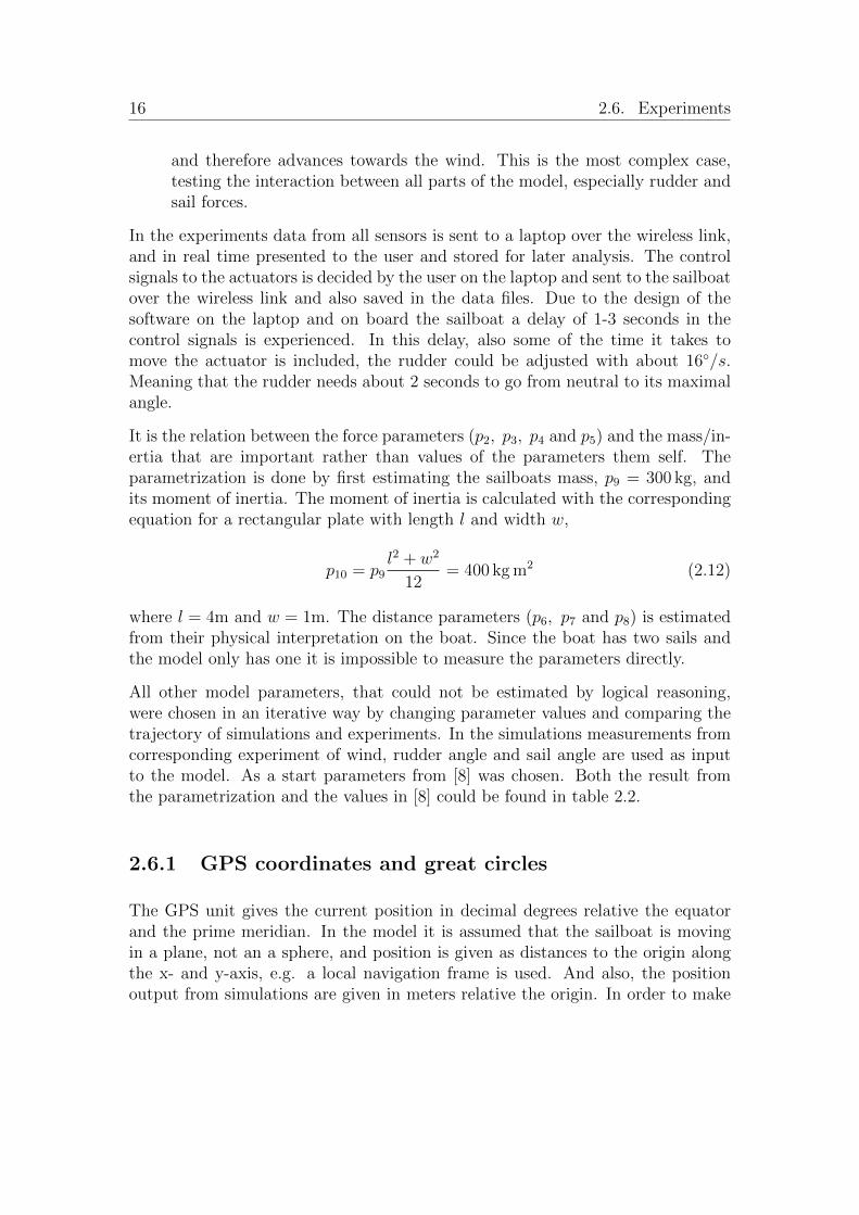
other controller than the sin-controller in equation 3.6 had been investigated. Thecontroller in both the simulation and the experiment were given the same pointsto construct a reference line from. The controller will steer the boat along thereference line from the starting point towards the points 1-6. The reference pointsare chosen with regards to the shape and obstacles present in the area were theexperiment were performed. The experiment lasted about 13 minutes, with awesterly wind of approximately 7 m/s.

In the figure, it can be seen that the sailboat in the simulation follows the referencenicely, but with statical control error downwind from the reference. The sailboatin experiment experienced big oscillations along the trajectory, especially in thebeginning. A possible explanation for this observation is a varying time-delay dueto, mainly, communication delays between the sailboat and the external laptop.If a time-delay is included in the model and simulated, similar oscillations canbe observed. Because of the oscillations, the maximum rudder angle in the con-troller, δr,max in equation 3.6, was changed from π/6 to π/9 after 300 seconds ofthe experiment. Although this clearly improved controller performance, the ex-periment shows the need for further improvement. Also, an obvious drawback ofthis modification is that maximum rudder can no longer be applied. The trial thusreveals the need to modify the “gain” of the controller without adjusting maxi-mum rudder angle. In figure 3.3 the control signal before and after the changein maximum rudder angle is shown. It is clear from the figure that the gain de-

Chapter 3. Control 27

−150 −100 −50 0 50 100 150

−30

−20

−10

0

10

20

30

e [deg]

u [d

eg]

usin

u2/3sin

Figure 3.3: Comparison of rudder angle as a function of the control error in theregion [−180◦ 180◦] for two sin-controllers with δr,max = π/6 solid (—) and δr,max = π/9dashed (– –).

creased together with the maximum rudder angle, the gain could be seen as theslope of the graph in the region around 0◦. It would be possible to manipulatethe control error, e.g. scaling with a constant, and in that way change the gainwithout changing the maximum rudder angle.

At this point in the project the other controllers were investigated with simulations.Due to limitations in available time for experiments no experiments with the othercontrollers were performed.

28 3.2. Rudder control evaluation

−300 −200 −100 0 100

−600

−500

−400

−300

−200

−100

0

100

x [m]

y [m

]

t= 757 s

experimentsimulationreference

300 s

start

1

2

4

5

6

3

Figure 3.4: Experiment with sin-controller compared with simulation. Desired trajec-tory, dotted (..), simulated path, dashed (– –), and experiment solid(—).

Chapter 4

State estimation

A desired feature of the autonomous system is a very low power consumptionduring longer missions. As discussed in [1], this can be achieved by shutting downthe measurement and control system for longer periods. Informed and safe choicesto shut down and wake up the electronic system can be based on reliable estimatesof the state of the boat, i.e., mainly the position. Given the form of the model andthe promising simulations, this chapter gives a hint of the possibilities for stateestimation with the use of Kalman filtering.

A Kalman filter is a method named after Rudolf E. Kalman whom was highlyinvolved in developing the theory. The aim of a Kalman filter is to improve mea-surements by filtering them with information about the underlying system pro-ducing the measurements and statistical information about noise included in themeasurements. The Kalman filter also gives the possibility to get an update of thestates without the need of new measurements. Since the model is non-linear anextended Kalman filter is used.

Kalman and extended Kalman filtering is widely used in many areas of controland signal processing. The following theory of this chapter is explained in greaterdetail, for example in [4, 5].

Two filters are introduced, one for filtering the measurements of apparent windand a second filter is used for the system states. The filtered wind measurementsare used as input to the sailboat system filter. The reason for using two separatefilters is stability. It turns out to be much easier to get a stable filter if the windmodel and the sailboat model are separated into two separate filters. It is notexactly clear why the combined filter tends to be unstable, some possibilities arediscussed in chapter 5.

29

30 4.1. Sailboat filter

4.1 Sailboat filter

4.1.1 Discretization of model equations

The model as stated in equation 2.1 is given on continuous form. For filteringthe model must be discretized, e.g. the system model needs to be expressed ondiscrete form.

xk+1 = f(xk,uk) (4.1)

where x is the state vector, u is the control signals, f is the non-linear discretizedsystem equations and k marks the time step. Here the true wind parameters are

considered to be part of the control signals, u =[δr δs atw ψtw

]T.

The continuous derivative is approximated with

dx

dt=

xk+1 − xkT

(4.2)

where T is the system sampling time. Thus is the discretized system equations inequation 4.1,

f(xk,uk) =

xk + T (vk cos(θk) + p1atw cos(ψtw))yk + T (vk sin(θk) + p1atw sin(ψtw))

θk + Tωkvk + T (gs sin(δs)− gr sin(δr)− p2v2k)/p9

ωk

(4.3)

where the rudder and sail forces, gr and gs, are calculated in the same way as inthe continues model. A process noise qk will be added to all states. The processnoise is assumed to be white zero mean Gaussian, with covariance matrix Q. Q isa static diagonal matrix and an important design parameter in the filter. It couldbe interpreted as an estimate of the model errors.

Take special notice of the difference in the fifth row in the discretized model com-pared to the continuous model. Due to stability problems the rotational speedequation is simplified to, ωk+1 = ωk + qk. The source of the instability is thedamping term dependent of ω. The problem could be solved by decreasing thesampling/predict time or by simplifying the equation for ωk+1. If the discretizedmodel in equation (4.3) is simulated the model is only stable if the time step issmall, more precisely T < 0.04 s. In all filter implementations that follows the ori-entation θ is measured and there is no need of knowing ω, therefore the simplifiedversion of ωk+1 is chosen. Similar problems could arise from the damping term inthe equation for vk+1, but this term is not as sensitive.

Chapter 4. State estimation 31

4.1.2 Measurement equations

The measurement equations, describing the relation between states and measure-ment, is trivial for the model states, e.g. a one-to-one relation.

yk =

xyθv

= h(xk) =

xkykθkvk

(4.4)

All measurements are assumed to include some noise rk. The measurement noiseis assumed to be white zero mean Gaussian, with covariance matrix,

R =

σ2x 0 0 0

0 σ2y 0 0

0 0 σ2θ 0

0 0 0 σ2v

(4.5)

where σi is the standard deviation of measurement sensor i. It is the relationbetween R and Q that are important when designing the filter.

4.1.3 Extended Kalman filter equations

The whole non-linear system, with noise, system equations and measurement equa-tions is now,

xk+1 = f(xk,uk) + qk (4.6)

yk = h(xk) + rk (4.7)

The extended Kalman filter consists of two parts, a predict part and an updatepart. In the predict part the old states is used together with the model to get anestimate of what the states will be in next time step, equation 4.8. In the updatepart the measurements is used for estimating the states at the current time step,equation 4.14. The notation k|k − 1 should be interpreted as the value at time kwith measurements up to time k − 1.

Predict equations

xk|k−1 = f(xk−1|k−1,uk−1) (4.8)

Pk|k−1 = Fk−1Pk−1|k−1FTk−1 +Q (4.9)

Fk−1 =∂f(x,u)

∂x

∣∣∣∣xk−1,uk−1

(4.10)

32 4.2. Wind filter

where P is the state covariance matrix, FT is the transpose of F , and F is thesystems Jacobian, e.g. the linearized system equation matrix.

Update equationsIn the update part the measurements is taken into consideration by construct-ing the innovation, which is the differences between the real measurements andwhat the model predicts that the measurements should be, equation (4.11). Theinnovation covariance, equation (4.12) is then used to decide the Kalman gain,equation (4.13). It is now possible to update the state and its covariance matrixwith equation (4.14) and (4.15).

yk = zk − h(xk|k−1) (4.11)

Sk = HkPk|k−1HTk +Rk (4.12)

Kk = Pk|k−1HTk S−1k (4.13)

xk|k = xk|k−1 +Kkyk (4.14)

Pk|k = (I −KkHk)Pk|k−1 (4.15)

Hk =∂h(x)

∂x

∣∣∣∣xk|k−1

(4.16)

where zk is the latest measurements, S is the innovation covariance, K is theKalman gain, I is the identity matrix and H is the measurement Jacobian.

When the innovation is calculated the values of the angles must be checked. Onthe unit circle is the difference, e.g. shortest distance, between two angles neverlarger then π, therefore is it some times necessary to correct the innovation angles.This is done by subtracting or adding 2π if the angles is larger or smaller then ±π.This is the same thing as mapping the angles to its corresponding value in theinterval

[−π π

].

4.2 Wind filter

The wind filter is also implemented as a Kalman filter with the same filter equationsas above, but the model and measurement equations differ. The true wind isassumed to slowly vary according to a random walk in discrete-time, i.e.,[

atw(k + 1)

ψtw(k + 1)

]=

[atw(k) + qaψtw(k) + qψ

](4.17)

Chapter 4. State estimation 33

where a is used to denote the filtered estimate of a and q is Gaussian noise. Statesfor heading and sailboat speed are also added to the state vector. The wind modelis linear and therefore the system is given by,

xk+1 = Fxk + qk

yk = h(xk) + rk(4.18)

where x =[atw ψtw θ v

]T, F is an identity matrix and h(xk) =

[W T

p,aw θ v]T

.

True wind is assumed to slowly vary and therefore the corresponding process noiseis set to a small value. Giving Q and R matrices as follows,

Q =

0.001 0 0 0

0 0.0001 0 00 0 1 00 0 0 1

, R =

1 0 0 00 1 0 00 0 0.1 00 0 0 0.1

(4.19)

4.3 Filter implementation and results

The sailboat filter and the wind filter were implemented in MATLAB. The windfilter has been tested and used in real time, but was executed on an externallaptop, as previously described. For the implementation of the sailboat filter theequations in section 4.1.3 is used, even though it would be possible to use a toolbox,for example [5].

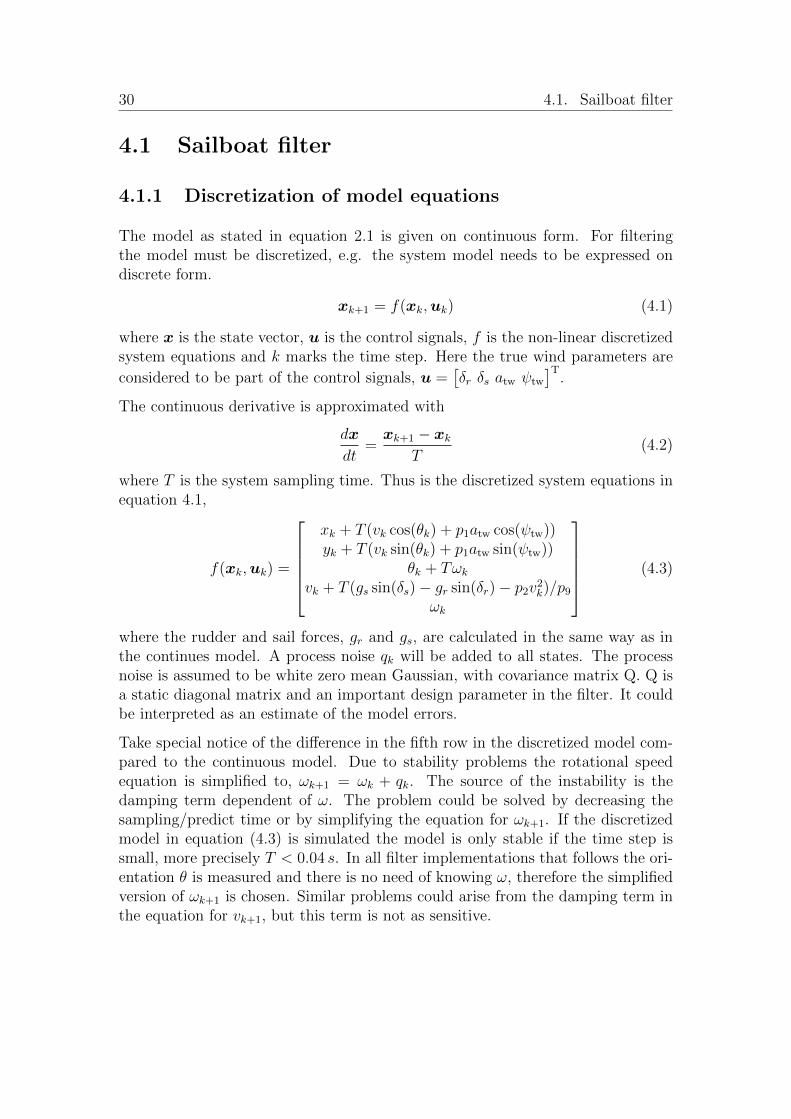
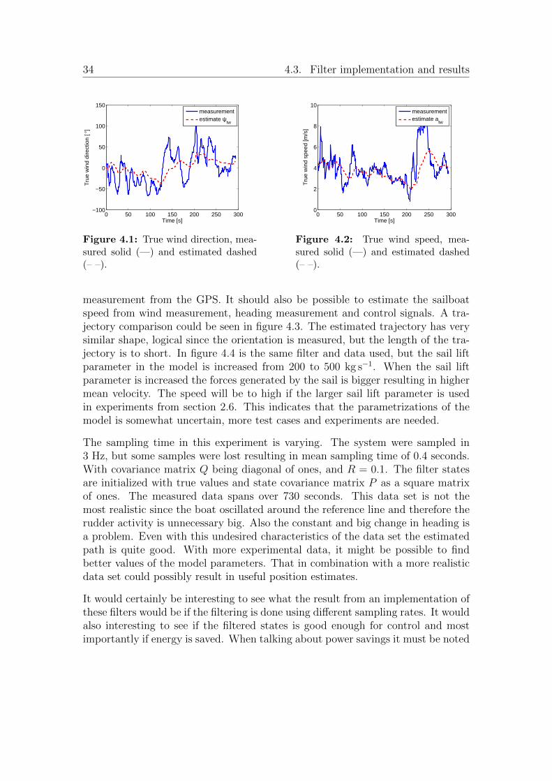
In figure 4.1 and 4.2 the filtered estimates of true wind can been seen togetherwith true wind measurements. True wind measurements are calculated with datafrom the wind sensor, compass and GPS unit. The filtered data spans over 300seconds and were collected during the controller experiment, same experiment asin figure 3.4. During this experiment the true wind was estimated from the windfilter developed here and used as input to the controller. Also for the same timeand approximate location, the Finnish Meteorogical Institue provided a westerlywind direction (0◦) and speed of 5 − 6 m/s, which correspond quite well to theestimates.

The sailboat filter in section 4.1 has been implemented with measurements of po-sition, orientation and boat speed. The output trajectory is almost identical tothe measured, just as expected. If the sailboat filter is implemented only withmeasurement from the compass, a more interesting filter is obtained when talkingabout power savings. Since this filter is not using the GPS. It should be notedthat the wind filter, that functions as input to the sailboat filter, needs the speed

34 4.3. Filter implementation and results

0 50 100 150 200 250 300−100

−50

0

50

100

150

Time [s]

Tru

e w

ind

dire

ctio

n [ °

]

measurementestimate ψ

tw

Figure 4.1: True wind direction, mea-sured solid (—) and estimated dashed(– –).

0 50 100 150 200 250 3000

2

4

6

8

10

Time [s]

Tru

e w

ind

spee

d [m

/s]

measurementestimate a

tw

Figure 4.2: True wind speed, mea-sured solid (—) and estimated dashed(– –).

measurement from the GPS. It should also be possible to estimate the sailboatspeed from wind measurement, heading measurement and control signals. A tra-jectory comparison could be seen in figure 4.3. The estimated trajectory has verysimilar shape, logical since the orientation is measured, but the length of the tra-jectory is to short. In figure 4.4 is the same filter and data used, but the sail liftparameter in the model is increased from 200 to 500 kg s−1. When the sail liftparameter is increased the forces generated by the sail is bigger resulting in highermean velocity. The speed will be to high if the larger sail lift parameter is usedin experiments from section 2.6. This indicates that the parametrizations of themodel is somewhat uncertain, more test cases and experiments are needed.

The sampling time in this experiment is varying. The system were sampled in3 Hz, but some samples were lost resulting in mean sampling time of 0.4 seconds.With covariance matrix Q being diagonal of ones, and R = 0.1. The filter statesare initialized with true values and state covariance matrix P as a square matrixof ones. The measured data spans over 730 seconds. This data set is not themost realistic since the boat oscillated around the reference line and therefore therudder activity is unnecessary big. Also the constant and big change in heading isa problem. Even with this undesired characteristics of the data set the estimatedpath is quite good. With more experimental data, it might be possible to findbetter values of the model parameters. That in combination with a more realisticdata set could possibly result in useful position estimates.

It would certainly be interesting to see what the result from an implementation ofthese filters would be if the filtering is done using different sampling rates. It wouldalso interesting to see if the filtered states is good enough for control and mostimportantly if energy is saved. When talking about power savings it must be noted

Chapter 4. State estimation 35

−400 −200 0 200 400−600

−500

−400

−300

−200

−100

0

x [m]

y [m

]

estmimatemeasured

Figure 4.3: Trajectory from experi-ment solid (—) and sailboat filter out-put dashed (– –) when sail lift pa-rameter set to its default value, p4 =200kg s−1.

−400 −200 0 200 400−600

−500

−400

−300

−200

−100

0

x [m]

y [m

]

estmimatemeasured

Figure 4.4: Trajectory from experi-ment solid (—) and sailboat filter out-put dashed (– –) with sail lift parameterincreased, p4 = 500kg s−1.

that the power consumption of the electronic system in this setup is negligible incomparison with power used by the actuators. But the steering system could bereplaced with something using less electrical power, e.g. a wind wane steeringsystem.

36 4.3. Filter implementation and results

Chapter 5

Concluding remarks

5.1 Conclusions and discussion

The developed model of the sailboat is rather simple with few parameters andfive states, the model captures the main characteristics of a sailboat quite well, asis observed in experiments. It should also be said that there is room for betterparametrization of the model, by the use of better data, longer data sets and moreaccurate measurements of rudder angle, and perhaps also an increased number oftest cases.

The model seems to capture characteristics of the sailboat well enough for thepurpose of controller design. Even though the controller that first was developedand tested with simulations showed bad behaviour when tested in an experiment.It is likely that the occurring oscillations would disappear if the controller is im-plemented exclusively in the on-board system since this would remove the timedelay related to the wireless link. If the time delay is removed the decision of whatrudder angle to use will be based on more resent data and therefore more accuratedata. Also the time between a decision and actual movement of an actuator willdecrease. A smaller time delay makes it easier to design a controller that steer thesailboat in a smooth way. Another way of dealing with the problem is to integratea time delay in the model, and thus making it possible developing controllers ca-pable of handling the time delays. This solutions is certainly not optimal since itdeals with the effect of the problem rather than the source of the problem. Andon a long mission is it absolutely necessary to have the controller implemented inthe on-board system.

In order to further explore the non-linear features of the boat and compare con-

37

38 5.1. Conclusions and discussion

trollers, more experiments under different conditions are required. Such experi-ments, for example in different wind speeds and wave heights, would likely havean effect on the values of the model parameters. It could for example be obvi-ous that some of the parameters are dependent on the wind speed and thereforebetter illustrating weaknesses in the model. Other experiment cases could alsoprovided useful information, e.g. sailing with wind from behind. If new, longer ex-periments are performed conclusion about the models performance could be madewith greater certainty. Especially the cases Circle and Straight line would benefitfrom longer data sets. 40 seconds seemed as a long time during the experiment,but when the data were analysed, and especially when talking about power savingsthis is a short time period, thus longer data sets are needed. The time periodsthat gives good results when shutting down and restarting a system/sensors forpower saving purposes is likely in the regions of minutes or possible hours.

The parametrization was done by visually comparing the trajectories and speedprofiles of experiments and simulations. This method is time consuming and notvery accurate. If a cost function is introduced the parametrization process could bemore effective and the result would likely be much better. Another benefit is thatthe result will be reproducible. The cost function could, for example, be a weightedsum of the squared error of the lateral trajectory and the speed profile.

The controller has not been tested during tacking with any experiments. Thealgorithm should work, since it has been tested in simulations, but experimentscould reveal weaknesses in the algorithm or some parameters that needs tuning.It is not clear how well the algorithm performs when the wind is coming from andirection close to the no-go zone, and if the wind is alternatively inside and outsideof the no-go zone.

In chapter 4, it is obvious that the wind measurement needs to be filtered, fig-ure 4.1. The method used seems to produce good estimates of true wind, atleast good enough for the control algorithm presented. Other, simpler methodscould also provide a good estimate of true wind, e.g. mean filtering of true windcalculations.

The developed sailboat filter is close to an open-loop simulation of the model. Itseems that a remaining challenge is to reliably estimate position as illustrated bythe growing difference between observations and simulations in figure 4.4. Con-sidering the endeavours connected to navigational satellite systems and the vastefforts under millennia of human civilization it is not, however, surprising thatGPS measurements are vital for accurate position estimation. Still, it seems thatwind and other state estimates can be used in open water to greatly decrease sam-pling rates and thus electrical power consumption. When a study of power savings

Chapter 5. Concluding remarks 39

is performed with practical experiments the sate estimation filter should also becompared with estimates based on constant speed and heading.

As mentioned earlier the decision of making two filters were based on problemswith stability in the filters. It is not exactly clear what the source of the problemsare, but when the discretized model is simulated a relatively short time periodbetween samples is needed, less than 0.04 seconds. Most of the time the problemstarts in the equation for ω, especially the friction term which will be very bigwhen ω is big. The friction term will also have alternating signs as the state goesto infinity. An other reason could be the way the discretization is done, otherand perhaps more suitable methods exist. It is of course also possible that theproblems solely lies within the implementation.

5.2 Further work

Recommendations for future work based on the findings of this thesis.

� Further experiments with the controllers integrated in the on-board system,in order to get an better understanding of the limitations of the model forcontroller development.

� Development of state estimation filters that can handle sensors with differentfrequencies. This kind of state estimation filters should then be used for anevaluation of the power saving strategy developed in [1].

� With an increased number of test cases and better data sets the parametriza-tion and evaluation of the model should be of better quality and the resultsand usefulness of the model will likely increase.

� Improve the system, both software in the external laptop and in the on-board system, with the time-delays in mind. Some sort of interrupt basedstrategies could be applied. This would further increase the benefits of thewireless link and facilitate fast controller development.

40 5.2. Further work

Bibliography

[1] K. Dahl, A. Bengsen, and M. Waller. Power management strategies for anautonomous robotic sailboat. In Robotic Sailing 2014: Proceedings of the 7thInternational Robotic Sailing Conference, pages 47–56. Springer, 2014.

[2] Ronny Eriksson and Anna Friebe. Challenges for autonomous sailing robots.In 14th Conference on Computer and IT Applications in the Maritime Indus-tries (COMPIT), pages 67–73, 2015.

[3] T.I. Fossen. Marine Control Systems: Guidance, Navigation and Control ofShips, Rigs and Underwater Vehicles. Marine Cybernetics, 2002.

[4] Fredrik Gustafsson. Statistical sensor fusion. Studentlitteratur, Lund, 2012.

[5] Jouni Hartikainena, Arno Solin, and Simo Sarkka. Optimal filtering withkalman filters and smoothers - a manual for the matlab toolbox ekf/ukf, 2011.http://becs.aalto.fi/en/research/bayes/ekfukf/documentation.pdf {2015-03-24}.

[6] Steffen Hessberger. Modeling and simulation of an autonomous sailing boat.Bachelor thesis, ETH Zurich, Switzerland, 2014.

[7] Luc Jaulin and Fabrice Le Bars. A simple controller for line following of sail-boats. In Robotic Sailing 2012: Proceedings of the 5th International RoboticSailing Conference, pages 117–129. Springer, 2012.

[8] Luc Jaulin and Fabrice Le Bars. Sailboat as a windmill. In Robotic Sailing2013: Proceedings of the 6th International Robotic Sailing Conference, pages81–92. Springer, 2013.

[9] David Krammer. Modeling and control of autonomous sailing boats. Master’sthesis, ETH Zurich, Switzerland, 2014.

[10] Robin Lovelock. Team Joker, Snoopy’s GPS Guided Trans-Atlantic RobotBoat, 2015. http://www.tsogpss.co.uk.gridhosted.co.uk/autop.htm {2015-04-21}.

41

42 Bibliography

[11] J. Melin, K. Dahl, and M. Waller. Modeling and control for an autonomoussailboat: A case study. In Robotic Sailing 2015: Proceedings of the 8th Inter-national Robotic Sailing Conference. Springer, 2015.

[12] Microtransat organisation. The microtransat challenge, 2015.http://www.microtransat.org {2015-06-21}.

[13] Roland Stelzer. Autonomous Sailboat Navigation, Novel Algorithms and Ex-perimental Demonstration. PhD thesis, De Montfort University, Leicester,United Kingdom, 2012.

[14] Roland Stelzer and Karim Jafarmadar. History and recent developmentsin robotic sailing. In Robotic Sailing: Proceedings of the 4th InternationalRobotic Sailing Conference, pages 3–23. Springer, 2011.

[15] Lin Xiao and Jerome Jouffroy. Modeling and nonlinear heading control ofsailing yachts. IEEE Journal of Oceanic Engineering, 39(2):256–268, 2014.