McGraw-Hill/Irwin © The McGraw-Hill Companies, Inc., 2003 15.1 Table of Contents Chapter 15...
58
© The McGraw-Hill Companies, Inc., 2003 15.1 McGraw-Hill/Irwin Table of Contents Chapter 15 (Computer Simulation: Basic Concepts) The Essence of Computer Simulation (Section 15.1) 15.2 Example 1: A Coin-Flipping Game (Section 15.1) 15.3–15.7 Example 2: Heavy Duty Company (Section 15.1) 15.8–15.14 Generating Observations from a Probability Distribution (Section 15.1) 15.15– 15.22 A Case Study: Herr Cutter’s Barber Shop (Section 15.2)15.23–15.29 Analysis of the Case Study (Section 15.3) 15.30–15.37 Some Common Types of Applications (Section 15.4) 15.38–15.39 Outline of a Major Computer Simulation Study (Section 15.5)15.40–15.42 Introduction to Simulation (UW Lecture) 15.43–15.58 These slides are based upon a lecture from the MBA core course in Management Science at the University of Washington (as taught by one of the authors).
-
Upload
jason-lucas -
Category
Documents
-
view
216 -
download
1
Transcript of McGraw-Hill/Irwin © The McGraw-Hill Companies, Inc., 2003 15.1 Table of Contents Chapter 15...
© The McGraw-Hill Companies, Inc., 200315.1McGraw-Hill/Irwin
Table of ContentsChapter 15 (Computer Simulation: Basic Concepts)
The Essence of Computer Simulation (Section 15.1) 15.2Example 1: A Coin-Flipping Game (Section 15.1) 15.3–15.7Example 2: Heavy Duty Company (Section 15.1) 15.8–15.14Generating Observations from a Probability Distribution (Section 15.1) 15.15–15.22A Case Study: Herr Cutter’s Barber Shop (Section 15.2) 15.23–15.29Analysis of the Case Study (Section 15.3) 15.30–15.37Some Common Types of Applications (Section 15.4) 15.38–15.39Outline of a Major Computer Simulation Study (Section 15.5) 15.40–15.42
Introduction to Simulation (UW Lecture) 15.43–15.58These slides are based upon a lecture from the MBA core course in Management Science at the University of Washington (as taught by one of the authors).
© The McGraw-Hill Companies, Inc., 200315.2McGraw-Hill/Irwin
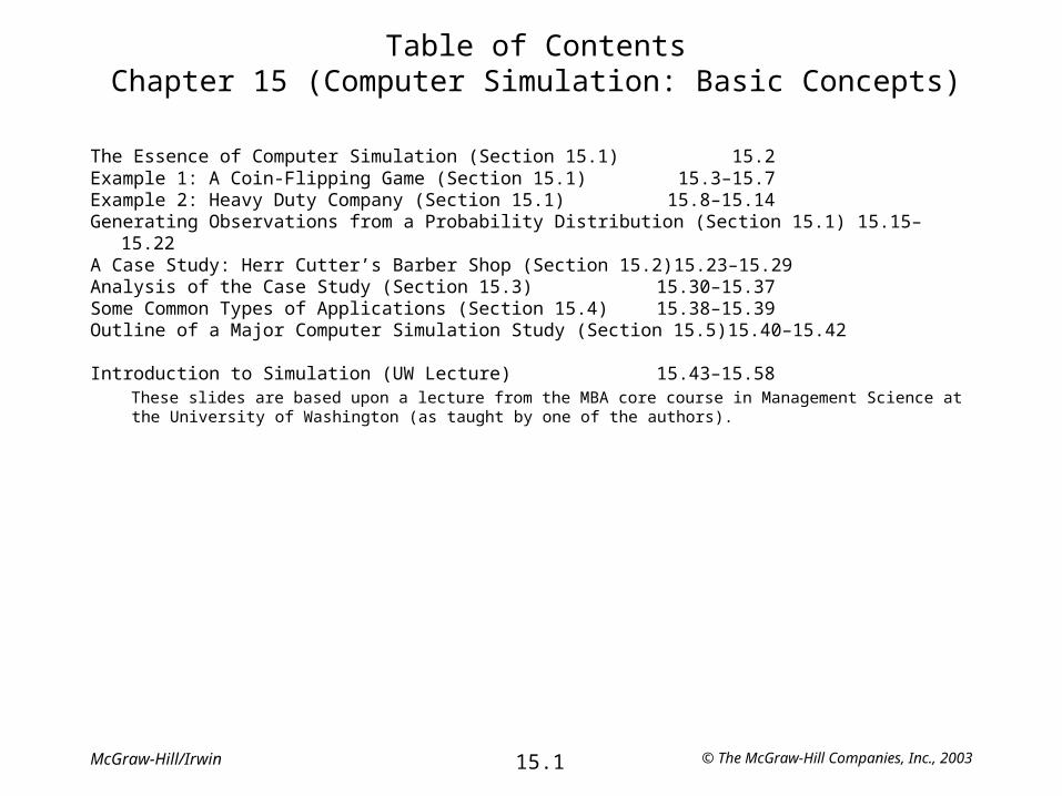
The Essence of Computer Simulation
• A stochastic system is a system that evolves over time according to one or more probability distributions.
• Computer simulation imitates the operation of such a system by using the corresponding probability distributions to randomly generate the various events that occur in the system.
• Rather than literally operating a physical system, the computer just records the occurrences of the simulated events and the resulting performance of the system.
• Computer simulation is typically used when the stochastic system ivolved is too complex to be analyzed satisfactorily by analytical models.
© The McGraw-Hill Companies, Inc., 200315.3McGraw-Hill/Irwin
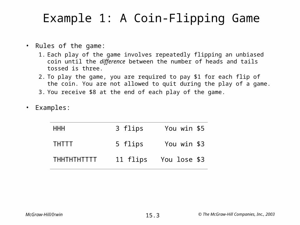
Example 1: A Coin-Flipping Game
• Rules of the game:1. Each play of the game involves repeatedly flipping an unbiased coin until the
difference between the number of heads and tails tossed is three.
2. To play the game, you are required to pay $1 for each flip of the coin. You are not allowed to quit during the play of a game.
3. You receive $8 at the end of each play of the game.
• Examples:
HHH 3 flips You win $5
THTTT 5 flips You win $3
THHTHTHTTTT 11 flips You lose $3
© The McGraw-Hill Companies, Inc., 200315.4McGraw-Hill/Irwin
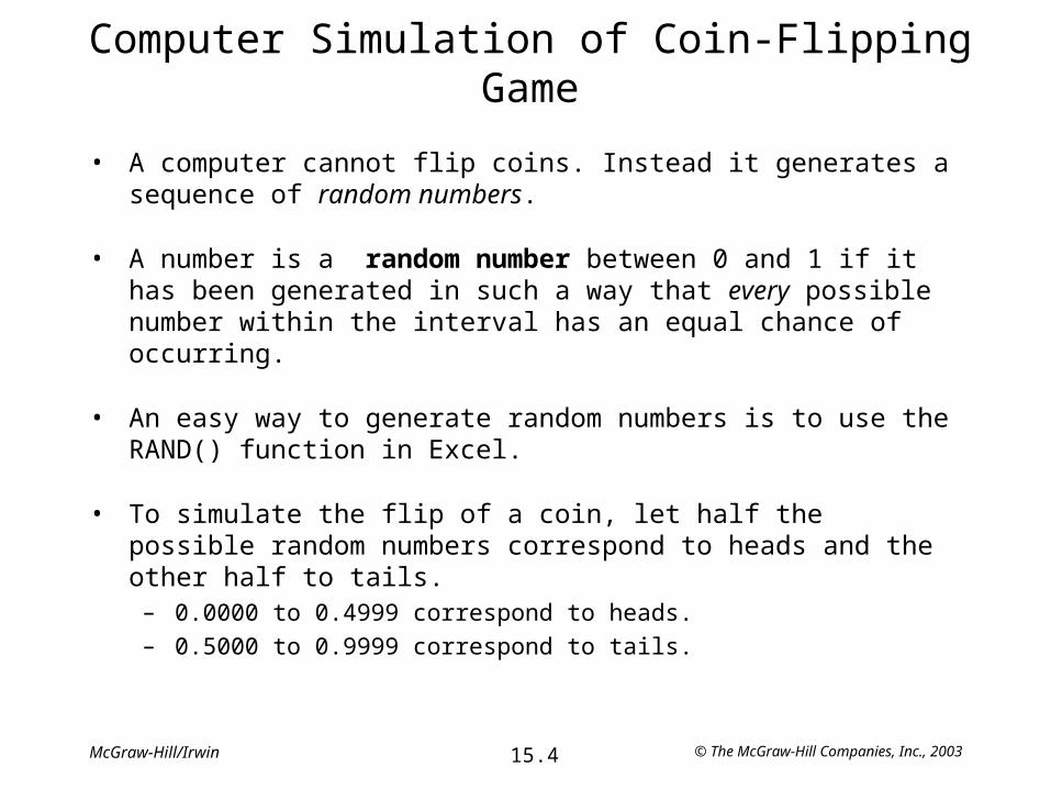
Computer Simulation of Coin-Flipping Game
• A computer cannot flip coins. Instead it generates a sequence of random numbers.
• A number is a random number between 0 and 1 if it has been generated in such a way that every possible number within the interval has an equal chance of occurring.
• An easy way to generate random numbers is to use the RAND() function in Excel.
• To simulate the flip of a coin, let half the possible random numbers correspond to heads and the other half to tails.
– 0.0000 to 0.4999 correspond to heads.
– 0.5000 to 0.9999 correspond to tails.
© The McGraw-Hill Companies, Inc., 200315.5McGraw-Hill/Irwin
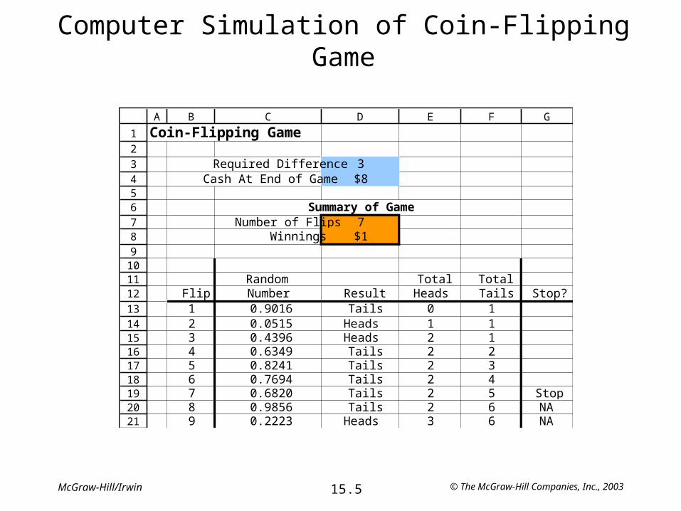
Computer Simulation of Coin-Flipping Game
123456789101112131415161718192021
A B C D E F G
Coin-Flipping Game
Required Difference 3Cash At End of Game $8
Summary of GameNumber of Flips 7
Winnings $1
Random Total TotalFlip Number Result Heads Tails Stop?1 0.9016 Tails 0 12 0.0515 Heads 1 13 0.4396 Heads 2 14 0.6349 Tails 2 25 0.8241 Tails 2 36 0.7694 Tails 2 47 0.6820 Tails 2 5 Stop8 0.9856 Tails 2 6 NA9 0.2223 Heads 3 6 NA

© The McGraw-Hill Companies, Inc., 200315.6McGraw-Hill/Irwin
Data Table for 14 Replications of Coin-Flipping Game
1
2
345678910111213141516171819202122
I J K L M
Data Table for Coin-Flipping Game(14 Replications)
NumberPlay of Flips Winnings
7 $11 19 -$112 5 $33 3 $54 11 -$35 9 -$16 5 $37 5 $38 3 $59 3 $5
10 5 $311 5 $312 5 $313 9 -$114 3 5
Average 6.43 $1.57
Select the whole table (J6:L20), before choosing Table from the Data menu.
© The McGraw-Hill Companies, Inc., 200315.7McGraw-Hill/Irwin
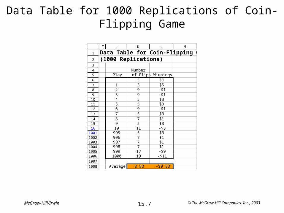
Data Table for 1000 Replications of Coin-Flipping Game
1
2
345678910111213141516
10011002100310041005100610071008
I J K L M
Data Table for Coin-Flipping Game(1000 Replications)
NumberPlay of Flips Winnings
5 $31 3 $52 9 -$13 9 -$14 5 $35 5 $36 9 -$17 5 $38 7 $19 5 $3
10 11 -$3995 5 $3996 7 $1997 7 $1998 7 $1999 17 -$91000 19 -$11
Average 8.83 -$0.83
© The McGraw-Hill Companies, Inc., 200315.8McGraw-Hill/Irwin
Corrective Maintenance versus Preventive Maintenance
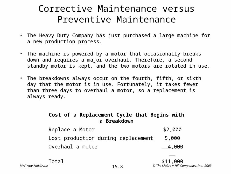
• The Heavy Duty Company has just purchased a large machine for a new production process.
• The machine is powered by a motor that occasionally breaks down and requires a major overhaul. Therefore, a second standby motor is kept, and the two motors are rotated in use.
• The breakdowns always occur on the fourth, fifth, or sixth day that the motor is in use. Fortunately, it takes fewer than three days to overhaul a motor, so a replacement is always ready.
Cost of a Replacement Cycle that Begins with a Breakdown
Replace a Motor $2,000
Lost production during replacement 5,000
Overhaul a motor 4,000
Total $11,000
© The McGraw-Hill Companies, Inc., 200315.9McGraw-Hill/Irwin
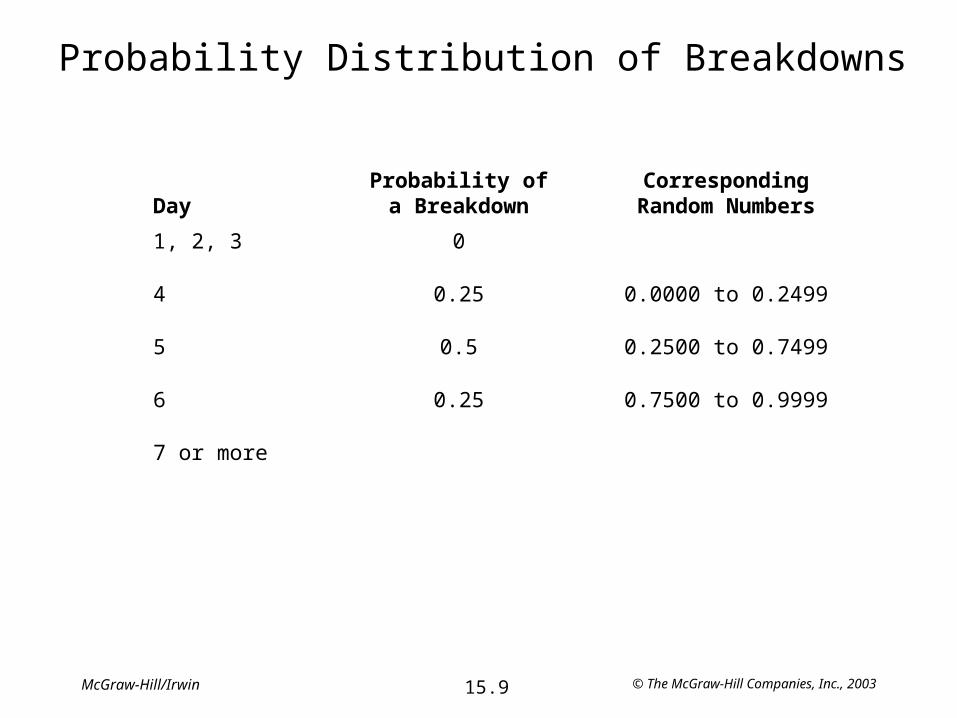
Probability Distribution of Breakdowns
DayProbability ofa Breakdown
CorrespondingRandom Numbers
1, 2, 3 0
4 0.25 0.0000 to 0.2499
5 0.5 0.2500 to 0.7499
6 0.25 0.7500 to 0.9999
7 or more
© The McGraw-Hill Companies, Inc., 200315.10McGraw-Hill/Irwin
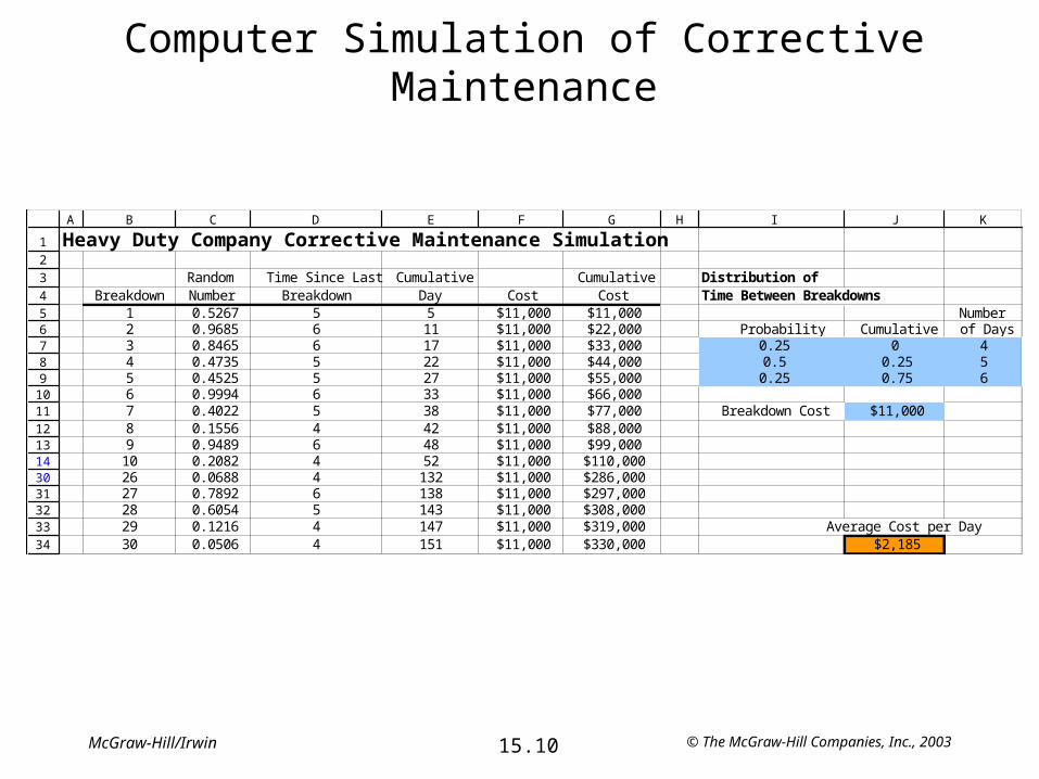
Computer Simulation of Corrective Maintenance
12345678910111213143031323334
A B C D E F G H I J K
Heavy Duty Company Corrective Maintenance Simulation
Random Time Since Last Cumulative Cumulative Distribution of Breakdown Number Breakdown Day Cost Cost Time Between Breakdowns
1 0.5267 5 5 $11,000 $11,000 Number2 0.9685 6 11 $11,000 $22,000 Probability Cumulative of Days3 0.8465 6 17 $11,000 $33,000 0.25 0 44 0.4735 5 22 $11,000 $44,000 0.5 0.25 55 0.4525 5 27 $11,000 $55,000 0.25 0.75 66 0.9994 6 33 $11,000 $66,0007 0.4022 5 38 $11,000 $77,000 Breakdown Cost $11,0008 0.1556 4 42 $11,000 $88,0009 0.9489 6 48 $11,000 $99,000
10 0.2082 4 52 $11,000 $110,00026 0.0688 4 132 $11,000 $286,00027 0.7892 6 138 $11,000 $297,00028 0.6054 5 143 $11,000 $308,00029 0.1216 4 147 $11,000 $319,000 Average Cost per Day30 0.0506 4 151 $11,000 $330,000 $2,185
© The McGraw-Hill Companies, Inc., 200315.11McGraw-Hill/Irwin
Preventive Maintenance Options
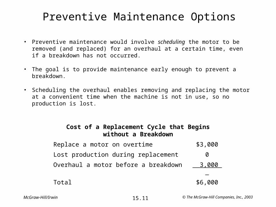
• Preventive maintenance would involve scheduling the motor to be removed (and replaced) for an overhaul at a certain time, even if a breakdown has not occurred.
• The goal is to provide maintenance early enough to prevent a breakdown.
• Scheduling the overhaul enables removing and replacing the motor at a convenient time when the machine is not in use, so no production is lost.
Cost of a Replacement Cycle that Begins without a Breakdown
Replace a motor on overtime $3,000
Lost production during replacement 0
Overhaul a motor before a breakdown 3,000
Total $6,000
© The McGraw-Hill Companies, Inc., 200315.12McGraw-Hill/Irwin
Replace Motor After 3 Days
• Cost of a replacement cycle is $6,000. (Replacement always occurs without a breakdown).
• Replacement cycle occurs every three days.
• E(Cost per day) = ($6,000) / (3 days) = $2,000 per day.
© The McGraw-Hill Companies, Inc., 200315.13McGraw-Hill/Irwin
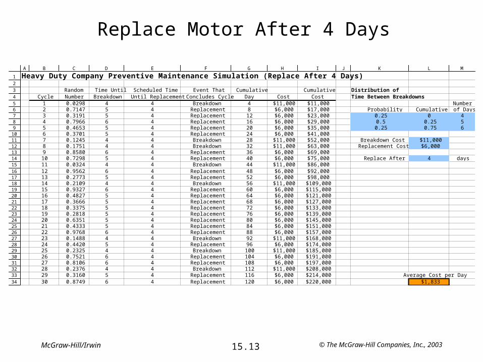
Replace Motor After 4 Days
12345678910111213141516171819202122232425262728293031323334
A B C D E F G H I J K L M
Heavy Duty Company Preventive Maintenance Simulation (Replace After 4 Days)
Random Time Until Scheduled Time Event That Cumulative Cumulative Distribution of Cycle Number Breakdown Until Replacement Concludes Cycle Day Cost Cost Time Between Breakdowns
1 0.0298 4 4 Breakdown 4 $11,000 $11,000 Number2 0.7147 5 4 Replacement 8 $6,000 $17,000 Probability Cumulative of Days3 0.3191 5 4 Replacement 12 $6,000 $23,000 0.25 0 44 0.7966 6 4 Replacement 16 $6,000 $29,000 0.5 0.25 55 0.4653 5 4 Replacement 20 $6,000 $35,000 0.25 0.75 66 0.3701 5 4 Replacement 24 $6,000 $41,0007 0.1245 4 4 Breakdown 28 $11,000 $52,000 Breakdown Cost $11,0008 0.1751 4 4 Breakdown 32 $11,000 $63,000 Replacement Cost $6,0009 0.8580 6 4 Replacement 36 $6,000 $69,00010 0.7298 5 4 Replacement 40 $6,000 $75,000 Replace After 4 days11 0.0324 4 4 Breakdown 44 $11,000 $86,00012 0.9562 6 4 Replacement 48 $6,000 $92,00013 0.2773 5 4 Replacement 52 $6,000 $98,00014 0.2109 4 4 Breakdown 56 $11,000 $109,00015 0.9327 6 4 Replacement 60 $6,000 $115,00016 0.4827 5 4 Replacement 64 $6,000 $121,00017 0.3666 5 4 Replacement 68 $6,000 $127,00018 0.3375 5 4 Replacement 72 $6,000 $133,00019 0.2818 5 4 Replacement 76 $6,000 $139,00020 0.6351 5 4 Replacement 80 $6,000 $145,00021 0.4333 5 4 Replacement 84 $6,000 $151,00022 0.9768 6 4 Replacement 88 $6,000 $157,00023 0.1488 4 4 Breakdown 92 $11,000 $168,00024 0.4420 5 4 Replacement 96 $6,000 $174,00025 0.2325 4 4 Breakdown 100 $11,000 $185,00026 0.7521 6 4 Replacement 104 $6,000 $191,00027 0.8106 6 4 Replacement 108 $6,000 $197,00028 0.2376 4 4 Breakdown 112 $11,000 $208,00029 0.3160 5 4 Replacement 116 $6,000 $214,000 Average Cost per Day30 0.8749 6 4 Replacement 120 $6,000 $220,000 $1,833
© The McGraw-Hill Companies, Inc., 200315.14McGraw-Hill/Irwin
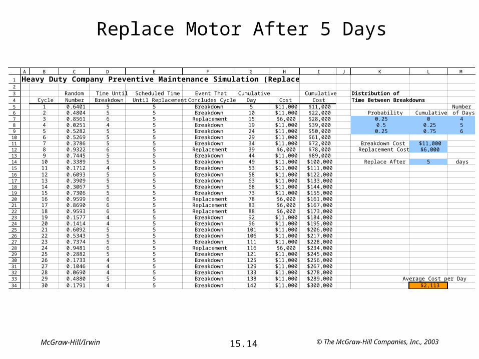
Replace Motor After 5 Days
12345678910111213141516171819202122232425262728293031323334
A B C D E F G H I J K L M
Heavy Duty Company Preventive Maintenance Simulation (Replace After 5 Days)
Random Time Until Scheduled Time Event That Cumulative Cumulative Distribution of Cycle Number Breakdown Until Replacement Concludes Cycle Day Cost Cost Time Between Breakdowns
1 0.6401 5 5 Breakdown 5 $11,000 $11,000 Number2 0.4804 5 5 Breakdown 10 $11,000 $22,000 Probability Cumulative of Days3 0.8561 6 5 Replacement 15 $6,000 $28,000 0.25 0 44 0.0251 4 5 Breakdown 19 $11,000 $39,000 0.5 0.25 55 0.5282 5 5 Breakdown 24 $11,000 $50,000 0.25 0.75 66 0.5269 5 5 Breakdown 29 $11,000 $61,0007 0.3786 5 5 Breakdown 34 $11,000 $72,000 Breakdown Cost $11,0008 0.9322 6 5 Replacement 39 $6,000 $78,000 Replacement Cost $6,0009 0.7445 5 5 Breakdown 44 $11,000 $89,00010 0.3389 5 5 Breakdown 49 $11,000 $100,000 Replace After 5 days11 0.1712 4 5 Breakdown 53 $11,000 $111,00012 0.6093 5 5 Breakdown 58 $11,000 $122,00013 0.3909 5 5 Breakdown 63 $11,000 $133,00014 0.3067 5 5 Breakdown 68 $11,000 $144,00015 0.7306 5 5 Breakdown 73 $11,000 $155,00016 0.9599 6 5 Replacement 78 $6,000 $161,00017 0.8690 6 5 Replacement 83 $6,000 $167,00018 0.9593 6 5 Replacement 88 $6,000 $173,00019 0.1577 4 5 Breakdown 92 $11,000 $184,00020 0.1414 4 5 Breakdown 96 $11,000 $195,00021 0.6092 5 5 Breakdown 101 $11,000 $206,00022 0.5343 5 5 Breakdown 106 $11,000 $217,00023 0.7374 5 5 Breakdown 111 $11,000 $228,00024 0.9481 6 5 Replacement 116 $6,000 $234,00025 0.2882 5 5 Breakdown 121 $11,000 $245,00026 0.1733 4 5 Breakdown 125 $11,000 $256,00027 0.1046 4 5 Breakdown 129 $11,000 $267,00028 0.0690 4 5 Breakdown 133 $11,000 $278,00029 0.4880 5 5 Breakdown 138 $11,000 $289,000 Average Cost per Day30 0.1791 4 5 Breakdown 142 $11,000 $300,000 $2,113
© The McGraw-Hill Companies, Inc., 200315.15McGraw-Hill/Irwin
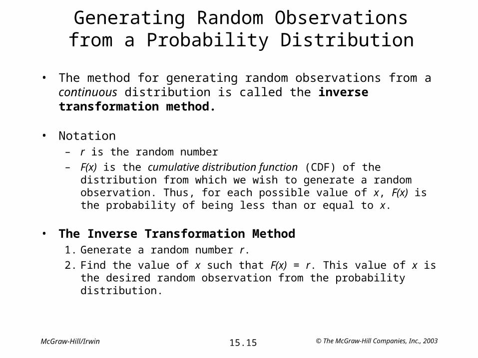
Generating Random Observationsfrom a Probability Distribution
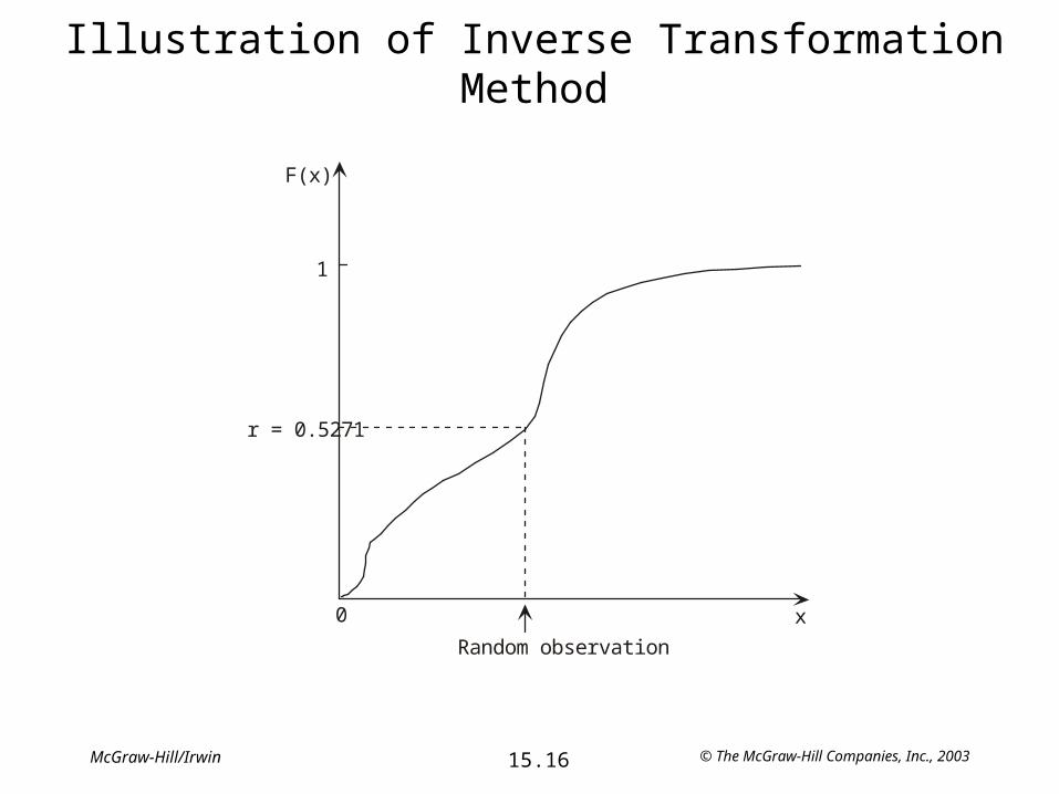
• The method for generating random observations from a continuous distribution is called the inverse transformation method.
• Notation– r is the random number
– F(x) is the cumulative distribution function (CDF) of the distribution from which we wish to generate a random observation. Thus, for each possible value of x, F(x) is the probability of being less than or equal to x.
• The Inverse Transformation Method1. Generate a random number r.
2. Find the value of x such that F(x) = r. This value of x is the desired random observation from the probability distribution.
© The McGraw-Hill Companies, Inc., 200315.16McGraw-Hill/Irwin
Illustration of Inverse Transformation Method
r = 0.5271
0
1
F(x)
x
Random observation
© The McGraw-Hill Companies, Inc., 200315.17McGraw-Hill/Irwin
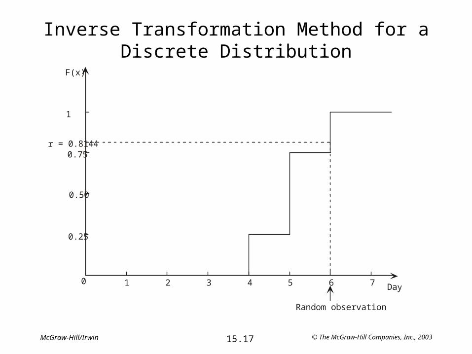
Inverse Transformation Method for a Discrete Distribution
F(x)
1
r = 0.8144
0.50
0.25
0 1 2 3 4 5 6 7 Day
Random observation
0.75
© The McGraw-Hill Companies, Inc., 200315.18McGraw-Hill/Irwin
Herr Cutter’s Barber Shop
• Herr Cutter is a German barber who runs a one-man barber shop. He opens his shop at 8:00 AM each weekday morning. His customers arrive randomly at an average rate of two customers per hour. He requires an average of 20 minutes for each haircut.
• As his business has increased, his customers now often wait awhile (sometimes over half-an-hour). His loyal customers are willing to wait, but new customers are much less likely to return if they have to wait.
• An article in The Barber’s Journal states– In a well-run barber shop, loyal customers will tolerate an average wait of 20
minutes, while new customers will tolerate only a 10 minute average wait. (With longer waits, they typically take their business elsewhere in the future.)
Question: Should Herr Cutter hire a new associate to share the workload?
© The McGraw-Hill Companies, Inc., 200315.19McGraw-Hill/Irwin
Probability Distributions
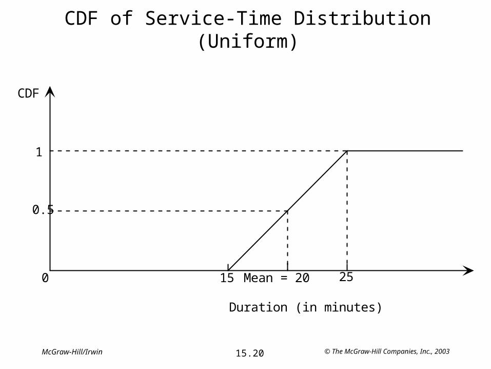
• The time required to give a haircut varies between 15 and 25 minutes. His best estimate is that the times between 15 and 25 minutes are equally likely.
– Estimated distribution of service times: The Uniform distribution over the interval from 15 to 25 minutes.
– The CDF for this distribution is P(service time ≤ x) = F(x) =
• 0 for x ≤ 15
• (x – 15)/10 for 15 ≤ x ≤ 25
• 1 for x ≥ 25
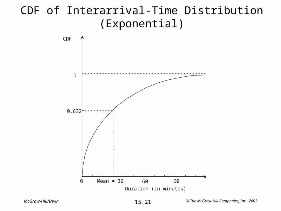
• The barber shop has random arrivals of customers, averaging two per hour.– Estimated distribution of interarrival times: An exponential distribution with a
mean of 30 minutes.
– The CDF for this distribution is P(interarrival time ≤ x) = F(x) =
• 1–e–x/30 for x ≥ 0.
© The McGraw-Hill Companies, Inc., 200315.20McGraw-Hill/Irwin
CDF of Service-Time Distribution (Uniform)
CDF
1
0.5
0 15 Mean = 20 25
Duration (in minutes)
© The McGraw-Hill Companies, Inc., 200315.21McGraw-Hill/Irwin
CDF of Interarrival-Time Distribution (Exponential)
1
0.632
0 Mean = 30 60 90
Duration (in minutes)
CDF

© The McGraw-Hill Companies, Inc., 200315.22McGraw-Hill/Irwin
Applying the Inverse Transformation Methodfor the Service Time (Uniform Distribution)
F(x)
1
r = 0.7270
0 15 Mean = 20 25
Random observation = 22.27
x
F(x) = (x–15)/10 = 0.7270 when x = 22.27
© The McGraw-Hill Companies, Inc., 200315.23McGraw-Hill/Irwin
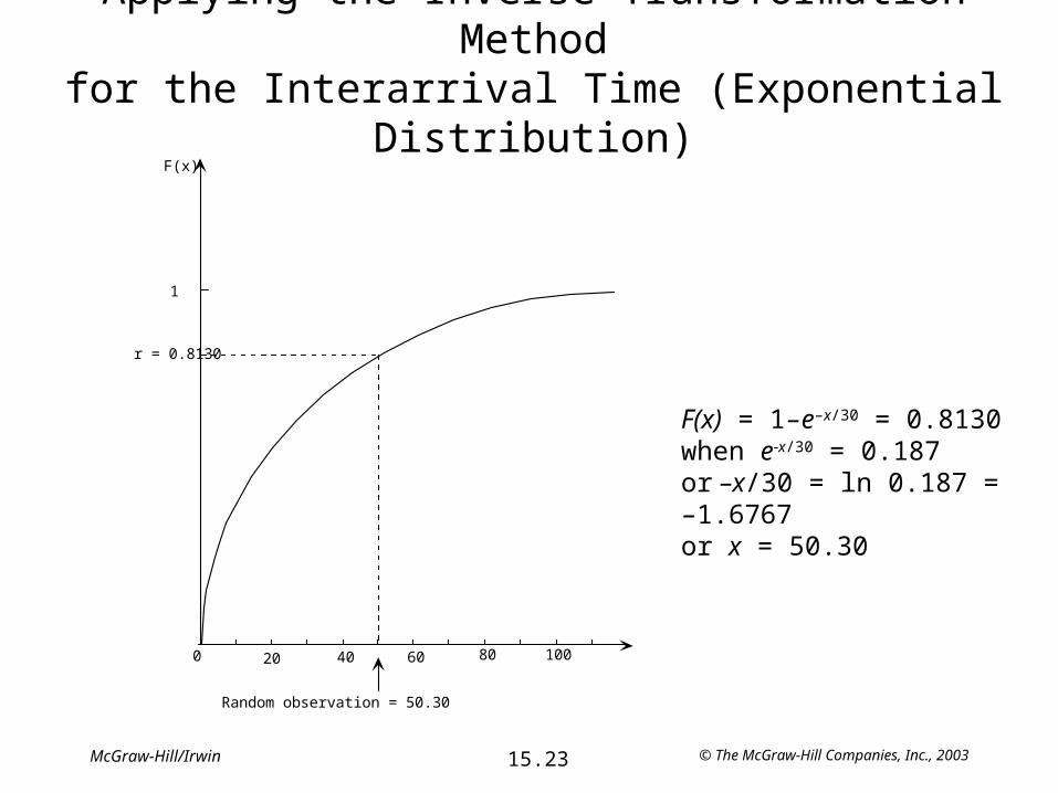
Applying the Inverse Transformation Methodfor the Interarrival Time (Exponential Distribution)
F(x) = 1–e–x/30 = 0.8130when e-x/30 = 0.187or –x/30 = ln 0.187 = –1.6767or x = 50.30
1
0 60 80
F(x)
r = 0.8130
1004020
Random observation = 50.30

© The McGraw-Hill Companies, Inc., 200315.24McGraw-Hill/Irwin
Building Blocks of a Simulation Model
1. A description of the components of the system, including how they are assumed to operate and interrelate.
2. A simulation clock.
3. A definition of the state of the system.
4. A method for randomly generating the (simulated) events that occur over time.
5. A method for changing the state of the system when an event occurs.
6. A procedure for advancing the time on the simulation clock.

© The McGraw-Hill Companies, Inc., 200315.25McGraw-Hill/Irwin
Building Blocks for Herr Cutter’s Simulation Model
1. A description of the components of the system, including how they are assumed to operate and interrelate.
• The components are the customers, the queue, and Herr Cutter as the server.
2. A simulation clock.• t = Amount of simulated time that has elapsed so far
3. A definition of the state of the system.• N(t) = Number of customers in the barber shop at time t.
4. A method for randomly generating the (simulated) events that occur over time.• The interarrival and service times are generated using the inverse transformation
method.
© The McGraw-Hill Companies, Inc., 200315.26McGraw-Hill/Irwin
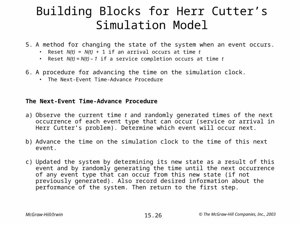
Building Blocks for Herr Cutter’s Simulation Model
5. A method for changing the state of the system when an event occurs.• Reset N(t) = N(t) + 1 if an arrival occurs at time t• Reset N(t) = N(t) – 1 if a service completion occurs at time t
6. A procedure for advancing the time on the simulation clock.• The Next-Event Time-Advance Procedure
The Next-Event Time-Advance Procedure
a) Observe the current time t and randomly generated times of the next occurrence of each event type that can occur (service or arrival in Herr Cutter’s problem). Determine which event will occur next.
b) Advance the time on the simulation clock to the time of this next event.
c) Updated the system by determining its new state as a result of this event and by randomly generating the time until the next occurrence of any event type that can occur from this new state (if not previously generated). Also record desired information about the performance of the system. Then return to the first step.

© The McGraw-Hill Companies, Inc., 200315.27McGraw-Hill/Irwin
A Computer Simulation of Herr Cutter’s Barber Shop
1234567891011121314151617181920
111112113114115
A B C D E F G H I
Herr Cutter's Barber Shop
(exponential)Mean Interarrival Time 30 minutes
(uniform)Min Service Time 15 minutes
Max Service Time 25 minutes
Average Time in Line (Wq) 14.1 minutesAverage Time in System (W) 34.0 minutes
Time Time Time Time TimeCustomer Interarrival of Service Service Service in in
Arrival Time Arrival Begins Time Ends Line System1 43.8 43.8 43.8 23.1 66.9 0.0 23.12 65.6 109.4 109.4 19.7 129.1 0.0 19.73 26.0 135.4 135.4 20.3 155.7 0.0 20.34 12.1 147.6 155.7 20.1 175.8 8.2 28.25 6.8 154.4 175.8 18.3 194.1 21.4 39.7
96 25.3 3,082.6 3,082.6 20.1 3,102.7 0.0 20.197 23.7 3,106.3 3,106.3 17.2 3,123.5 0.0 17.298 31.7 3,138.0 3,138.0 19.7 3,157.8 0.0 19.799 24.3 3,162.3 3,162.3 22.7 3,185.0 0.0 22.7
100 12.9 3,175.2 3,185.0 15.0 3,200.0 9.8 24.8

© The McGraw-Hill Companies, Inc., 200315.28McGraw-Hill/Irwin
Evolution of Number of Customers Over First 100 Minutes
20 40 60 80 100
1
2
3
Elapsed time (in minutes)
Number ofcustomers inthe system
© The McGraw-Hill Companies, Inc., 200315.29McGraw-Hill/Irwin
Simulating the Barber Shop with an Associate
• The only difference occurs when the next-event time-advance procedure is determining which event occurs next.
• Instead of just two possibilities, there are now three:1. A departure because Herr Cutter completes a haircut.
2. A departure because the associate completes a haircut.
3. An arrival.
© The McGraw-Hill Companies, Inc., 200315.30McGraw-Hill/Irwin
Analysis of the Case Study: Financial Factors
• Revenue = $15 per haircut
• Average tip = $2 per haircut
• Cost of maintaining the shop = $50 per working day
• Salary of an associate = $120 per working day
• Commission for an associate = $5 per haircut given by the associate.
• In addition to his salary and commission, the associate would keep his own tips. Otherwise, the revenue would go to Herr Cutter.
• The shop is open from 8:00 AM to 5:00 PM, so it admits customers for nine hours.
© The McGraw-Hill Companies, Inc., 200315.31McGraw-Hill/Irwin
Analysis of Continuing without an Associate
• The current distribution of interarrival times has a mean of 30 minutes. Therefore, he averages 18 customers per working day.
• After subtracting the cost of maintaining the shop, his average net income per working day is
Net daily income = ($15 + $2) (18 customers) – $50= $306 – $50= $256
© The McGraw-Hill Companies, Inc., 200315.32McGraw-Hill/Irwin
Features of the Queueing Simulator
1. Can run computer simulations of various kinds of basic queueing systems.
2. Can have any number of servers up to a maximum of 25.
3. Can use any of the following probability distributions for either interarrival times or service times:
a) Constant time (also called the degenerate distribution).
b) Exponential distribution.
c) Translated exponential distribution (the sum of a constant time and a time from an exponential distribution).
d) Uniform distribution.
e) Erlang distribution.
4. Provides estimates of various key measures of performance:L = Expected number of customers in the system, including those being served.
Lq = Expected number of customers in the queue.
W = Expected waiting time in the system (includes service time) for a customer.
Wq = Expected waiting time in the queue (excluding service time) for a customer.
Pn = Probability of exactly n customers in the system (for n = 1, 2, … , 10).

© The McGraw-Hill Companies, Inc., 200315.33McGraw-Hill/Irwin
Queueing Simulator for Herr Cutter (Without Associate)
3456789
101112131415161718192021
B C D E F G HData Results
Number of Servers = 1 PointEstimate Low High
Interarrival Times L = 1.358 1.332 1.385Distribution = Exponential Lq = 0.689 0.666 0.712
Mean = 30 W = 40.582 39.983 41.1805 Wq = 20.577 19.980 21.174
Service Times P0 = 0.330 0.326 0.335Distribution = Uniform P1 = 0.310 0.307 0.313
Minimum Value = 15 P2 = 0.183 0.180 0.185Maximum Value = 25 P3 = 0.0492 0.0920 0.0963
P4 = 0.0451 0.0433 0.0469Length of Simulation Run P5 = 0.0206 0.0192 0.0220
Number of Arrivals = 10,000 P6 = 0.00950 0.00849 0.01050P7 = 0.00432 0.00360 0.00503P8 = 0.00219 0.00163 0.00274P9 = 0.000876 0.000540 0.001210
P10 = 0.000372 0.000165 0.000579
95% Confidence Interval
Run Simulation

© The McGraw-Hill Companies, Inc., 200315.34McGraw-Hill/Irwin
Testing the Validity of the Simulation Model
123456789
10
1112
A B C D E F G
Template for the M/G/1 Queueing Model
Data Results 0.0333 (mean arrival rate) L = 1.344
20 (expected service time) Lq = 0.678 2.887 (standard deviation)s = 1 (# servers) W = 40.356
Wq = 20.356
0.666
P0 = 0.334
© The McGraw-Hill Companies, Inc., 200315.35McGraw-Hill/Irwin
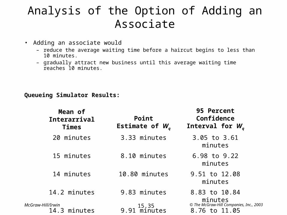
Analysis of the Option of Adding an Associate
• Adding an associate would– reduce the average waiting time before a haircut begins to less than 10 minutes.– gradually attract new business until this average waiting time reaches 10 minutes.
Queueing Simulator Results:
Mean ofInterarrival Times
PointEstimate of Wq
95 Percent ConfidenceInterval for Wq
20 minutes 3.33 minutes 3.05 to 3.61 minutes
15 minutes 8.10 minutes 6.98 to 9.22 minutes
14 minutes 10.80 minutes 9.51 to 12.08 minutes
14.2 minutes 9.83 minutes 8.83 to 10.84 minutes
14.3 minutes 9.91 minutes 8.76 to 11.05 minutes
© The McGraw-Hill Companies, Inc., 200315.36McGraw-Hill/Irwin
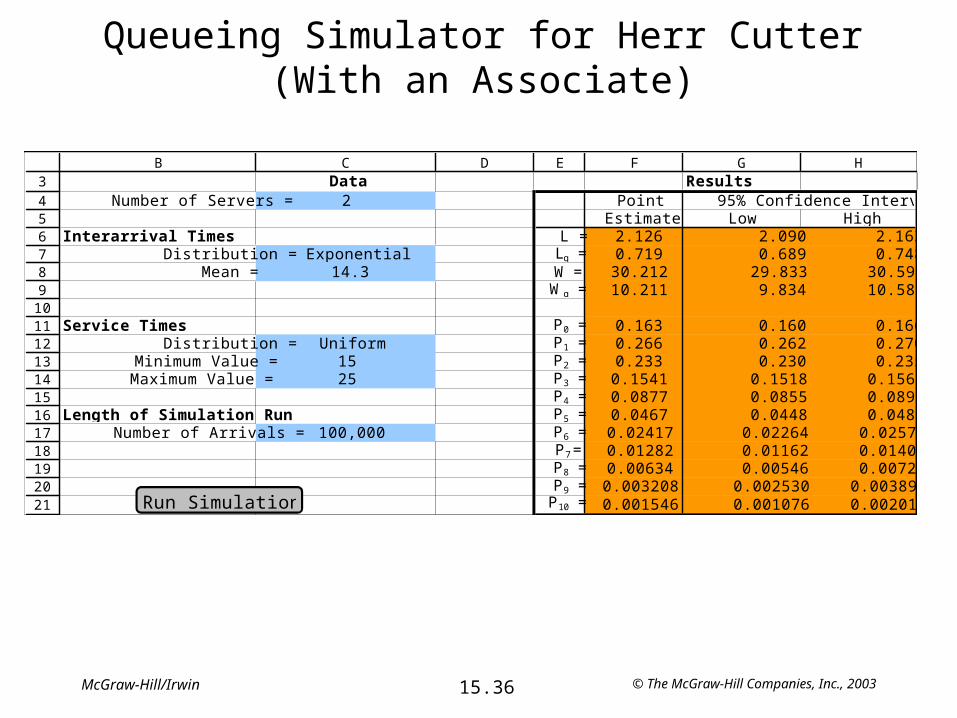
Queueing Simulator for Herr Cutter (With an Associate)
3456789
101112131415161718192021
B C D E F G HData Results
Number of Servers = 2 PointEstimate Low High
Interarrival Times L = 2.126 2.090 2.163Distribution = Exponential Lq = 0.719 0.689 0.748
Mean = 14.3 W = 30.212 29.833 30.5915 Wq = 10.211 9.834 10.588
Service Times P0 = 0.163 0.160 0.166Distribution = Uniform P1 = 0.266 0.262 0.270
Minimum Value = 15 P2 = 0.233 0.230 0.235Maximum Value = 25 P3 = 0.1541 0.1518 0.1564
P4 = 0.0877 0.0855 0.0898Length of Simulation Run P5 = 0.0467 0.0448 0.0487
Number of Arrivals = 100,000 P6 = 0.02417 0.02264 0.02570P7 = 0.01282 0.01162 0.01401P8 = 0.00634 0.00546 0.00722P9 = 0.003208 0.002530 0.003890
P10 = 0.001546 0.001076 0.002017
95% Confidence Interval
Run Simulation
© The McGraw-Hill Companies, Inc., 200315.37McGraw-Hill/Irwin
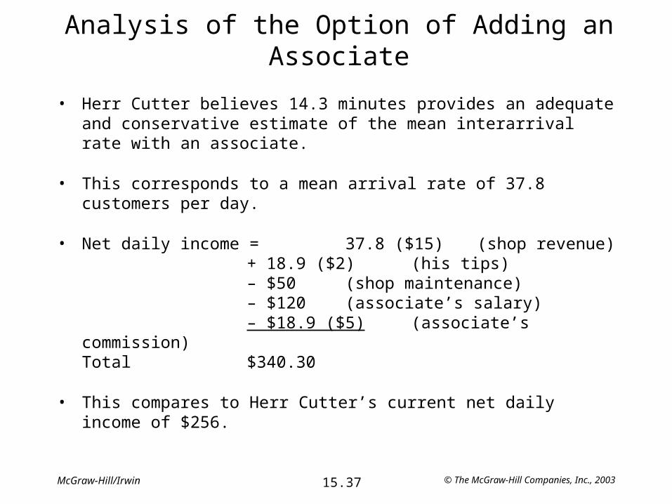
Analysis of the Option of Adding an Associate
• Herr Cutter believes 14.3 minutes provides an adequate and conservative estimate of the mean interarrival rate with an associate.
• This corresponds to a mean arrival rate of 37.8 customers per day.
• Net daily income = 37.8 ($15) (shop revenue)+ 18.9 ($2) (his tips)– $50 (shop maintenance)– $120 (associate’s salary)– $18.9 ($5) (associate’s commission)
Total $340.30
• This compares to Herr Cutter’s current net daily income of $256.
© The McGraw-Hill Companies, Inc., 200315.38McGraw-Hill/Irwin
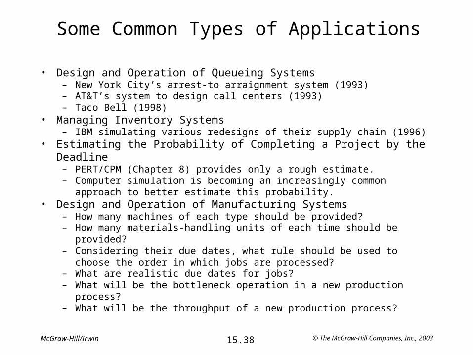
Some Common Types of Applications
• Design and Operation of Queueing Systems– New York City’s arrest-to arraignment system (1993)– AT&T’s system to design call centers (1993)– Taco Bell (1998)
• Managing Inventory Systems– IBM simulating various redesigns of their supply chain (1996)
• Estimating the Probability of Completing a Project by the Deadline– PERT/CPM (Chapter 8) provides only a rough estimate.– Computer simulation is becoming an increasingly common approach to better
estimate this probability.• Design and Operation of Manufacturing Systems
– How many machines of each type should be provided?– How many materials-handling units of each time should be provided?– Considering their due dates, what rule should be used to choose the order in which
jobs are processed?– What are realistic due dates for jobs?– What will be the bottleneck operation in a new production process?– What will be the throughput of a new production process?
© The McGraw-Hill Companies, Inc., 200315.39McGraw-Hill/Irwin
Some Common Types of Applications
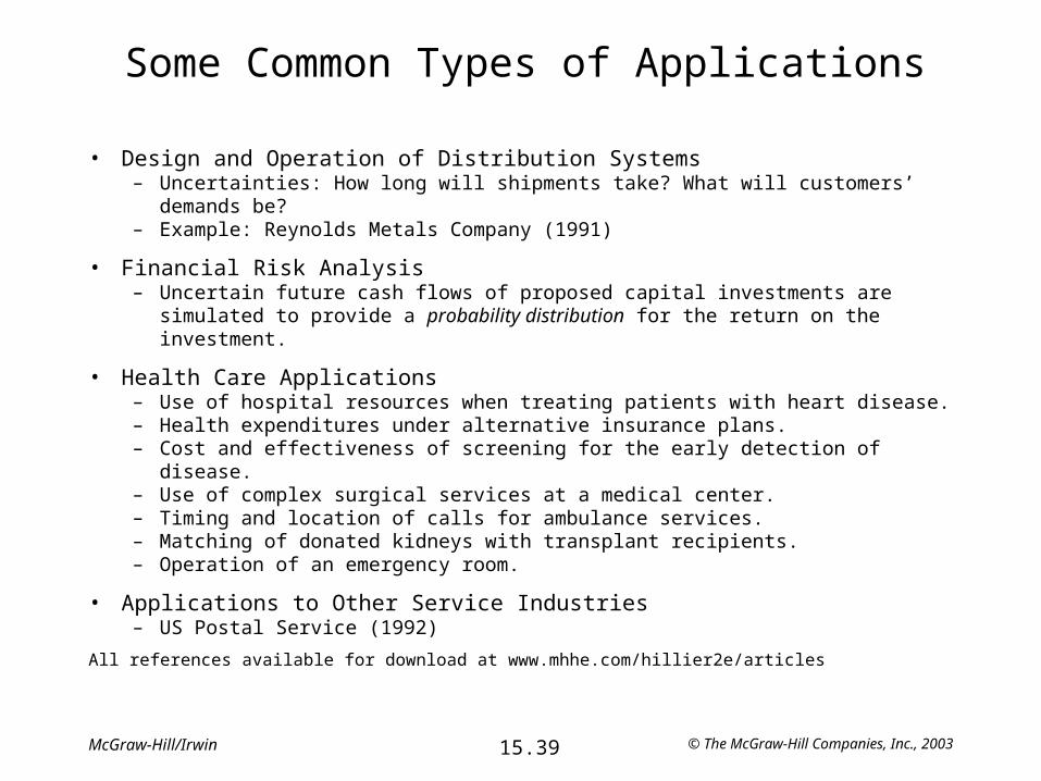
• Design and Operation of Distribution Systems– Uncertainties: How long will shipments take? What will customers’ demands be?– Example: Reynolds Metals Company (1991)
• Financial Risk Analysis– Uncertain future cash flows of proposed capital investments are simulated to
provide a probability distribution for the return on the investment.
• Health Care Applications– Use of hospital resources when treating patients with heart disease.– Health expenditures under alternative insurance plans.– Cost and effectiveness of screening for the early detection of disease.– Use of complex surgical services at a medical center.– Timing and location of calls for ambulance services.– Matching of donated kidneys with transplant recipients.– Operation of an emergency room.
• Applications to Other Service Industries– US Postal Service (1992)
All references available for download at www.mhhe.com/hillier2e/articles

© The McGraw-Hill Companies, Inc., 200315.40McGraw-Hill/Irwin
Outline of a Major Computer Simulation Study
• Step 1: Formulate the Problem and Plan the Study– What is the problem that management wants studied?
– What are the overall objectives for the study?
– What specific issues should be addressed?
– What kinds of alternative system configurations should be considered?
– What measures of performance of the system are of interest to management?
– What are the time constraints for performing the study?
• Step 2: Collect the Data and Formulate the Simulation Model– The probability distributions of the relevant quantities are needed.
– Generally it will only be possible to estimate these distributions.
– A simulation model often is formulated in terms of a flow diagram.
• Step 3: Check the Accuracy of the Simulation Model– Walk through the conceptual model before an audience of all the key people.

© The McGraw-Hill Companies, Inc., 200315.41McGraw-Hill/Irwin
Outline of a Major Computer Simulation Study
• Step 4: Select the Software and Construct a Computer Program– Classes of software
• Spreadsheet software (e.g., Excel, Crystal Ball)
• A general purpose programming language (e.g., C, FORTRAN, Pascal, etc.)
• A general purpose simulation language (e.g., GPSS, SIMSCRIPT, SLAM, SIMAN)
• Applications-oriented simulators
• Step 5: Test the Validity of the Simulation Model– If the real system is currently in operation, performance data should be compared
with the corresponding output generated by the simulation model.
– Conduct a field test to collect data to compare to the simulation model.
– Have knowledgeable personnel check how the simulation results change as the configuration of the simulated system is changed.
– Watch animations of simulation runs.
© The McGraw-Hill Companies, Inc., 200315.42McGraw-Hill/Irwin
Outline of a Major Computer Simulation Study
• Step 6: Plan the Simulations to Be Performed– Determine length of simulation runs.
– Keep in mind that the simulation runs do no produce exact values. Each simulation run can be viewed as a statistical experiment that is generating statistical observations of the performance of the system.
• Step 7: Conduct the Simulation Runs and Analyze the Results
– Obtain point estimates and confidence intervals to indicate the range of likely values for the measures.
• Step 8: Present Recommendations to Management
© The McGraw-Hill Companies, Inc., 200315.43McGraw-Hill/Irwin
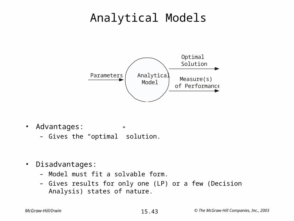
Analytical Models
Generating EPSF...Generating EPSF...Generating EPSF...Generating EPSF...Generating EPSF...Generating EPSF...Generating EPSF...
AnalyticalModel
Parameters
OptimalSolution
Measure(s)of Performance
• Advantages:– Gives the “optimal” solution.
• Disadvantages:– Model must fit a solvable form.
– Gives results for only one (LP) or a few (Decision Analysis) states of nature.

© The McGraw-Hill Companies, Inc., 200315.44McGraw-Hill/Irwin
Simulation Models
• Advantages:– Can include factors that cause problems in analytical models.
– Gives a distribution of results for many possible states of nature.
• Disadvantages:– Doesn’t give an “optimal solution”.
– Good at evaluating, but not finding, solutions.
Generating EPSF...Generating EPSF...Generating EPSF...Generating EPSF...Generating EPSF...Generating EPSF...Generating EPSF...
SimulationModel
Parameters
TrialSolution
Measure(s)of Performance
© The McGraw-Hill Companies, Inc., 200315.45McGraw-Hill/Irwin
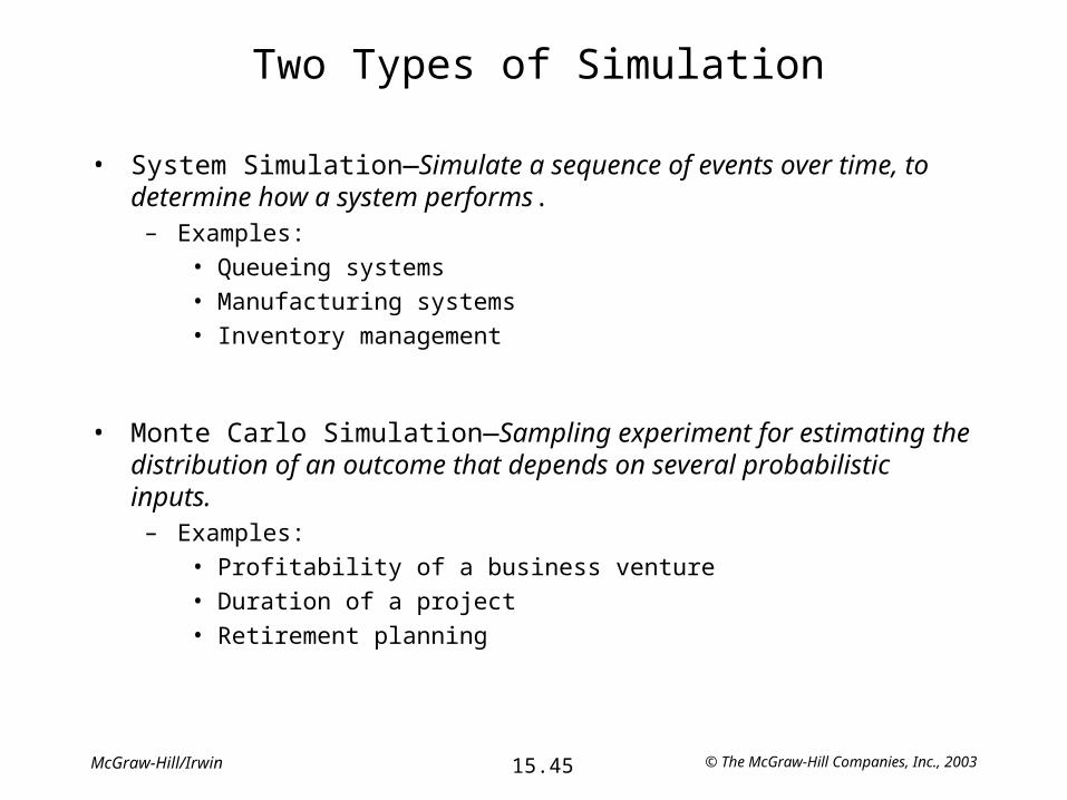
Two Types of Simulation
• System Simulation—Simulate a sequence of events over time, to determine how a system performs.
– Examples:
• Queueing systems
• Manufacturing systems
• Inventory management
• Monte Carlo Simulation—Sampling experiment for estimating the distribution of an outcome that depends on several probabilistic inputs.
– Examples:
• Profitability of a business venture
• Duration of a project
• Retirement planning
© The McGraw-Hill Companies, Inc., 200315.46McGraw-Hill/Irwin
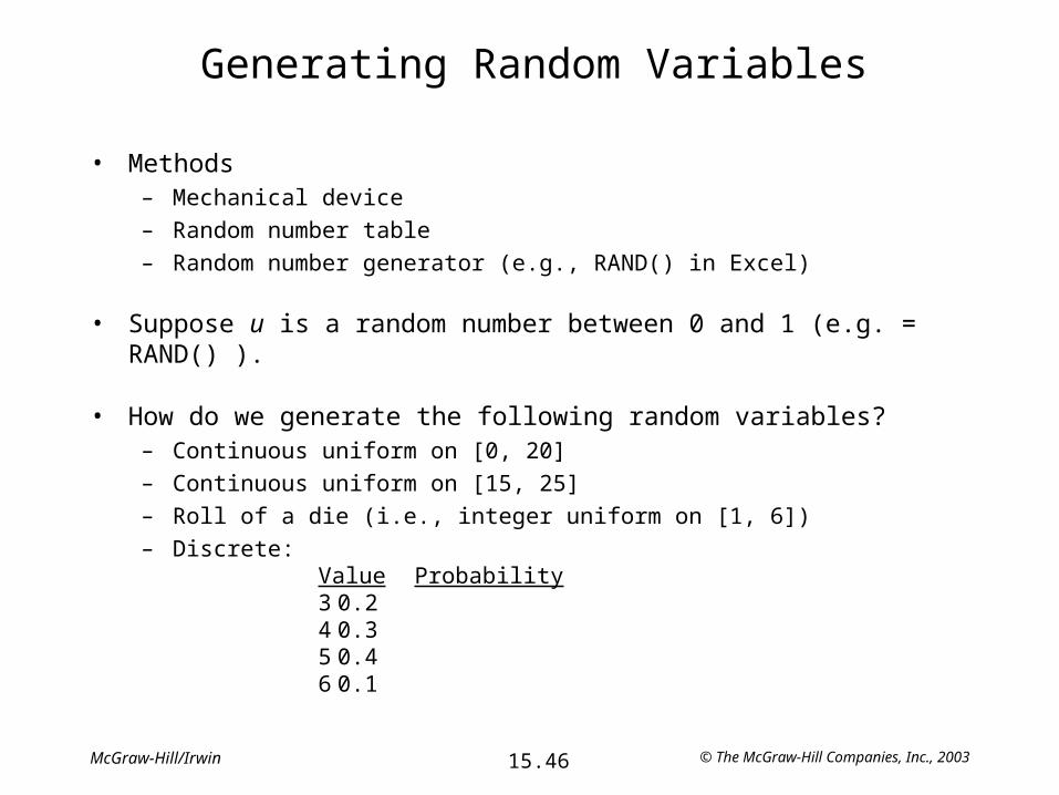
Generating Random Variables
• Methods– Mechanical device
– Random number table
– Random number generator (e.g., RAND() in Excel)
• Suppose u is a random number between 0 and 1 (e.g. = RAND() ).
• How do we generate the following random variables?– Continuous uniform on [0, 20]
– Continuous uniform on [15, 25]
– Roll of a die (i.e., integer uniform on [1, 6])
– Discrete:Value Probability
3 0.24 0.35 0.46 0.1
© The McGraw-Hill Companies, Inc., 200315.47McGraw-Hill/Irwin
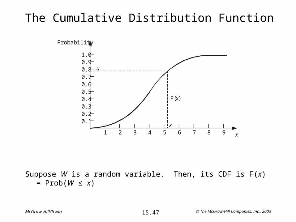
The Cumulative Distribution Function
Generating EPSF...Generating EPSF...Generating EPSF...Generating EPSF...Generating EPSF...Generating EPSF...Generating EPSF...Generating EPSF...Generating EPSF...Generating EPSF...Generating EPSF...Generating EPSF...Generating EPSF...Generating EPSF...Generating EPSF...Generating EPSF...Generating EPSF...Generating EPSF...Generating EPSF...Generating EPSF...Generating EPSF...Generating EPSF...Generating EPSF...Generating EPSF...Generating EPSF...Generating EPSF...Generating EPSF...Generating EPSF...Generating EPSF...Generating EPSF...Generating EPSF...Generating EPSF...Generating EPSF...Generating EPSF...Generating EPSF...Generating EPSF...Generating EPSF...Generating EPSF...Generating EPSF...Generating EPSF...Generating EPSF...Generating EPSF...Generating EPSF...Generating EPSF...
Probability
0.10.20.30.40.50.60.70.80.91.0
1 2 3 4 5 6 7 8 9 x
u
x
F(x)
Suppose W is a random variable. Then, its CDF is F(x) = Prob(W ≤ x)

© The McGraw-Hill Companies, Inc., 200315.48McGraw-Hill/Irwin
To Generate Any Continuous Random Variable
1. Generate u ~ Uniform [ 0, 1 ]
2. Find x for which F(x) = u.
3. Then x is the generated random variable.

© The McGraw-Hill Companies, Inc., 200315.49McGraw-Hill/Irwin
Generating Random Variables in Excel
• Uniform[a, b]= a + (b – a) * RAND()
• Discrete Uniform[a, b]= INT(a + (b - a + 1)*RAND() )
• Normal(, )= NORMINV(RAND(), , )
• Exponential (with rate = )=(–1/) * LN( RAND() )

© The McGraw-Hill Companies, Inc., 200315.50McGraw-Hill/Irwin
Freddie the Newsboy
• Freddie runs a newsstand in a prominent downtown location of a major city.
• Freddie sells a variety of newspapers and magazines. The most expensive of the newspapers is the Financial Journal.
• Cost data for the Financial Journal:– Freddie pays $1.50 per copy delivered.
– Freddie charges $2.50 per copy.
– Freddie’s refund is $0.50 per unsold copy.
• Sales data for the Financial Journal:– Freddie sells anywhere between 40 and 70 copies a day.
– The frequency of the numbers between 40 and 70 are roughly equal.
© The McGraw-Hill Companies, Inc., 200315.51McGraw-Hill/Irwin
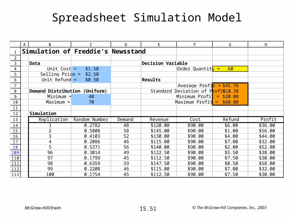
Spreadsheet Simulation Model
123456789
101112131415161718
109110111112113
A B C D E F G H
Simulation of Freddie's Newsstand
Data Decision VariableUnit Cost = $1.50 Order Quantity = 60
Selling Price = $2.50Unit Refund = $0.50 Results
Average Profit = $45.76Demand Distribution (Uniform) Standard Deviation of Profit = $12.38
Minimum = 40 Minimum Profit = $20.00Maximum = 70 Maximum Profit = $60.00
SimulationReplication Random Number Demand Revenue Cost Refund Profit
1 0.2782 48 $120.00 $90.00 $6.00 $36.002 0.5808 58 $145.00 $90.00 $1.00 $56.003 0.4103 52 $130.00 $90.00 $4.00 $44.004 0.2086 46 $115.00 $90.00 $7.00 $32.005 0.5371 56 $140.00 $90.00 $2.00 $52.00
96 0.3014 49 $122.50 $90.00 $5.50 $38.0097 0.1799 45 $112.50 $90.00 $7.50 $30.0098 0.6359 59 $147.50 $90.00 $0.50 $58.0099 0.2208 46 $115.00 $90.00 $7.00 $32.00
100 0.1754 45 $112.50 $90.00 $7.50 $30.00
© The McGraw-Hill Companies, Inc., 200315.52McGraw-Hill/Irwin
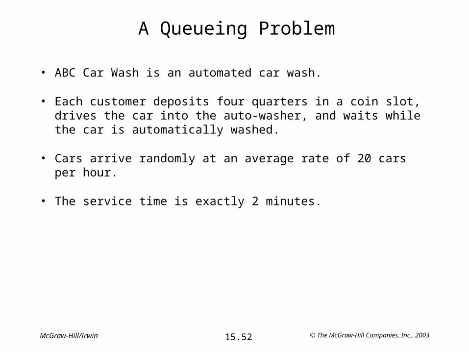
A Queueing Problem
• ABC Car Wash is an automated car wash.
• Each customer deposits four quarters in a coin slot, drives the car into the auto-washer, and waits while the car is automatically washed.
• Cars arrive randomly at an average rate of 20 cars per hour.
• The service time is exactly 2 minutes.
© The McGraw-Hill Companies, Inc., 200315.53McGraw-Hill/Irwin
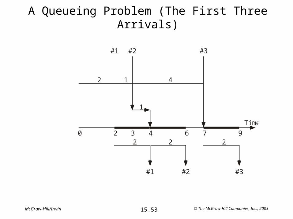
A Queueing Problem (The First Three Arrivals)
Generating EPSF...Generating EPSF...Generating EPSF...Generating EPSF...Generating EPSF...Generating EPSF...Generating EPSF...Generating EPSF...Generating EPSF...Generating EPSF...Generating EPSF...Generating EPSF...Generating EPSF...Generating EPSF...Generating EPSF...Generating EPSF...Generating EPSF...Generating EPSF...Generating EPSF...Generating EPSF...Generating EPSF...Generating EPSF...Generating EPSF...Generating EPSF...Generating EPSF...Generating EPSF...Generating EPSF...Generating EPSF...Generating EPSF...Generating EPSF...Generating EPSF...Generating EPSF...Generating EPSF...Generating EPSF...Generating EPSF...Generating EPSF...
#1 #2 #3
2 1 4
#1 #2 #3
2 2 20 2 4 6 7 9
Time
1
3
© The McGraw-Hill Companies, Inc., 200315.54McGraw-Hill/Irwin
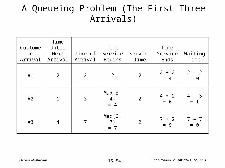
A Queueing Problem (The First Three Arrivals)
CustomerArrival
TimeUntil Next
ArrivalTime ofArrival
TimeServiceBegins
ServiceTime
TimeServiceEnds
WaitingTime
#1 2 2 2 22 + 2= 4
2 – 2= 0
#2 1 3Max(3, 4)
= 42
4 + 2= 6
4 – 3= 1
#3 4 7Max(6, 7)
= 72
7 + 2= 9
7 – 7= 0

© The McGraw-Hill Companies, Inc., 200315.55McGraw-Hill/Irwin
Queueing Problem Simulation Model
1
2
3
4
5
6
7
8
91011121314151617
507508509510511512
A B C D E F G H
Simulation of ABC Car Wash
Arrivals per minute = 0.33333333
Service time (minutes) = 2
Average Time in Line = 5.7 minutes
Standard Deviation = 6.4 minutes
Maximum Time in Line = 18.9 minutes
Time Time Time TimeCustomer Until Next Time of Service Service Service in
Arrival Arrival Arrival Begins Time Ends Line1 1.67 1.67 1.67 2.00 3.67 0.002 0.89 2.56 3.67 2.00 5.67 1.113 0.91 3.47 5.67 2.00 7.67 2.204 0.90 4.37 7.67 2.00 9.67 3.305 0.26 4.64 9.67 2.00 11.67 5.03
495 0.43 1472.93 1475.47 2.00 1477.47 2.54496 6.50 1479.44 1479.44 2.00 1481.44 0.00497 0.65 1480.08 1481.44 2.00 1483.44 1.35498 2.32 1482.40 1483.44 2.00 1485.44 1.03499 0.63 1483.04 1485.44 2.00 1487.44 2.40500 0.36 1483.39 1487.44 2.00 1489.44 4.04
© The McGraw-Hill Companies, Inc., 200315.56McGraw-Hill/Irwin
A Game of Craps
• A popular game in gambling casinos is the game of craps.
• In its most basic form, the game is played as follows:– A player rolls two dice and calculates the sum.
– If the sum is 7 or 11, the play wins right away.
– If the sum is 2, 3, or 12, the player loses right away.
– If the sum is any other number (4, 5, 6, 8, 9, or 10), the number becomes the player’s “point”.
• In this case, the dice are thrown repeatedly until the sum is either:
– the “point” (in which case the player wins), or
– 7 (in which case the player loses).
© The McGraw-Hill Companies, Inc., 200315.57McGraw-Hill/Irwin
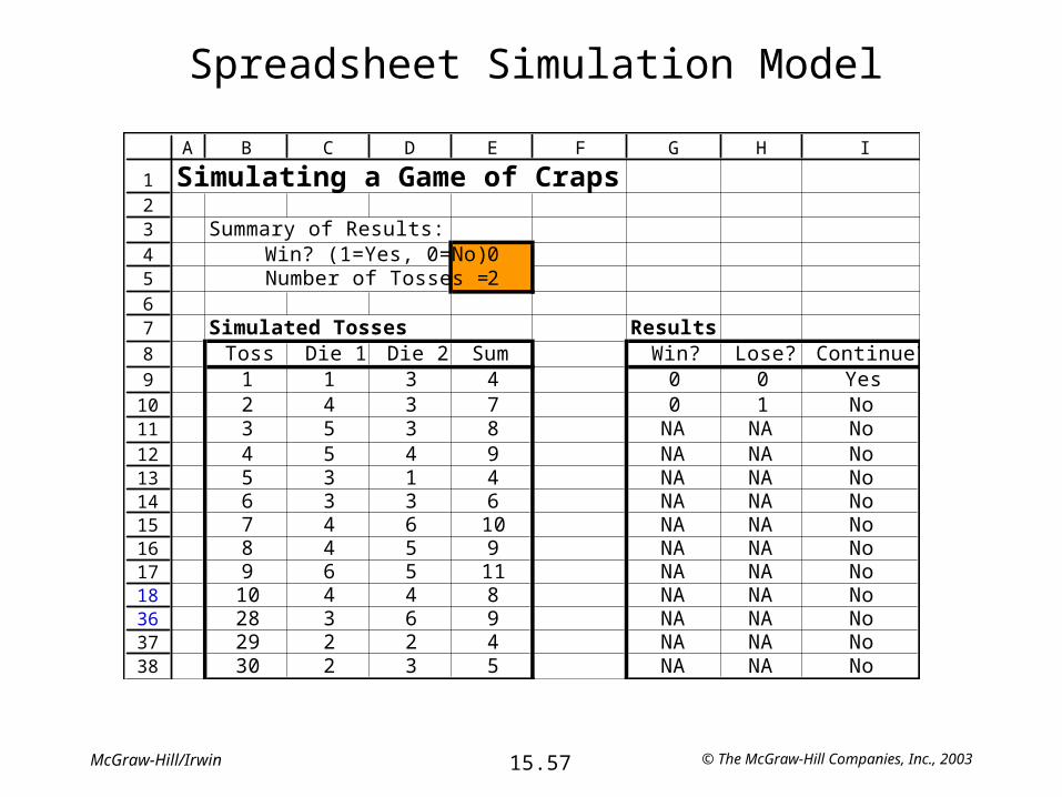
Spreadsheet Simulation Model
123456789101112131415161718363738
A B C D E F G H I
Simulating a Game of Craps
Summary of Results:Win? (1=Yes, 0=No) 0Number of Tosses = 2
Simulated Tosses ResultsToss Die 1 Die 2 Sum Win? Lose? Continue?
1 1 3 4 0 0 Yes2 4 3 7 0 1 No3 5 3 8 NA NA No4 5 4 9 NA NA No5 3 1 4 NA NA No6 3 3 6 NA NA No7 4 6 10 NA NA No8 4 5 9 NA NA No9 6 5 11 NA NA No
10 4 4 8 NA NA No28 3 6 9 NA NA No29 2 2 4 NA NA No30 2 3 5 NA NA No

© The McGraw-Hill Companies, Inc., 200315.58McGraw-Hill/Irwin
Using a Data Table to Perform Many Simulation Trials
1. In the first row of the table (row 12), put equations referring to the output cells of the simulation spreadsheet (=E4 in M12, =E5 in N12).
2. In the first column of the table, label each simulation trial (1 to 100).3. Select the entire table (L12 through N112).4. Choose Table from the Data menu.5. For the Column input cell, select any empty cell (e.g., K7).
123456789
1011121314151617
108109110111112
A B C D E F G H I J K L M N
Simulating a Game of Craps 100 Replications of Craps
Summary of Results: Bet per Game = $10Win? (1=Yes, 0=No) 1Number of Tosses = 3 Number of Wins = 47
Winnings = ($60)Simulated Tosses Results Average Number of Tosses = 3.23
Toss Die 1 Die 2 Sum Win? Lose? Continue?1 1 3 4 0 0 Yes Simulation2 4 5 9 0 0 Yes Number of3 3 1 4 1 0 No Game Win? Tosses4 1 1 2 NA NA No 1 35 4 5 9 NA NA No 1 1 16 3 4 7 NA NA No 2 1 27 2 5 7 NA NA No 3 0 48 6 1 7 NA NA No 4 0 69 5 2 7 NA NA No 5 0 5
96 0 297 0 798 1 199 0 3
100 0 2